Decay modes of the scalar exotic meson $T_{bs;\overline{u}\overline{d}}^{-}$

Abstract

We investigate the semileptonic decay of the scalar tetraquark $T_{bs;\overline{u}\overline{d}}^{-}$ to final state $T_{cs;\overline{u}\overline{d}}^{0}l\overline{\nu}_{l}$, which proceeds due to the weak transition $b\to cl\overline{\nu}_{l}$. For these purposes, we calculate the spectroscopic parameters of the final-state scalar tetraquark $T_{cs;\overline{u}\overline{d}}^{0}$. In calculations we use the QCD sum rule method by taking into account the quark, gluon, and mixed condensates up to dimension 10. The mass of the $T_{cs;\overline{u}\overline{d}}^{0}$ obtained in the present work $(2878\pm 128)~{}\mathrm{MeV}$ indicates that it is unstable against the strong interactions, and can decay to the mesons $D^{0}\overline{K}^{0}$ and $D^{+}K^{-}$. Partial widths of these $S$-wave modes as well as the full width of the tetraquark $T_{cs;\overline{u}\overline{d}}^{0}$ are found by means of the QCD light-cone sum rule method and technical tools of the soft-meson approximation. The partial widths of the main semileptonic processes $T_{bs;\overline{u}\overline{d}}^{-}\to T_{cs;\overline{u}\overline{d}}^{0}l\overline{\nu}_{l}$, $l=e,\mu$, and $\tau$ are computed by employing the weak form factors $G_{1}(q^{2})$ and $G_{2}(q^{2})$, which are extracted from the QCD three-point sum rules. We also trace back the weak transformations of the stable tetraquark $T_{bb;\overline{u}\overline{d}}^{-}$ to conventional mesons. The obtained results for the full width $\Gamma_{\mathrm{full}}=(3.28\pm 0.60)\times 10^{-10}~{}\mathrm{MeV}$ and mean lifetime $\tau=2.01_{-0.31}^{+0.44}~{}\mathrm{ps}$ of $T_{bs;\overline{u}\overline{d}}^{-}$, as well as predictions for decay channels of the tetraquark $T_{bb;\overline{u}\overline{d}}^{-}$ can be used in experimental studies of these exotic states.

I Introduction

Investigation of exotic mesons composed of four valence quarks, i.e., tetraquarks is one of the interesting and intriguing problems on agenda of high energy physics. Experimental data collected by various collaborations and achievements in their theoretical explanations made these states an important part of hadron spectroscopy Chen:2016qju ; Chen:2016spr ; Esposito:2016noz ; Ali:2017jda ; Olsen:2017bmm . But the nonstandard mesons discovered till now and considered as candidates to exotics are wide resonances which decay strongly to conventional mesons. These circumstances obscure their four-quark bound-state nature and inspire appearance of alternative dynamical models to account for observed effects. Therefore, theoretical and experimental studies of 4-quark states, which are stable against the strong interactions can be decisive for distinguishing dynamical effects and genuine multiquark states from each another.

The problems of stability of 4-quark mesons were already addressed in the original papers Ader:1981db ; Lipkin:1986dw ; Zouzou:1986qh . The principal conclusion made in these works was that, if a mass ratio $m_{Q}/m_{q}$ is large, then the heavy $Q$ and light $q$ quarks may constitute stable $QQ\bar{q}\bar{q}$ compounds. The stabile nature of the axial-vector tetraquark $T_{bb;\overline{u}\overline{d}}^{-}$ (briefly, $T_{bb}^{-}$) was predicted in Ref. Carlson:1987hh , and confirmed by recent investigations Navarra:2007yw ; Karliner:2017qjm ; Eichten:2017ffp . The similar conclusions about the strong-interaction stability of the tetraquarks $T_{bb;\overline{u}\overline{s}}^{-}$, and $T_{bb;\overline{d}\overline{s}}^{0}$ were drawn in Ref. Eichten:2017ffp as well. The spectroscopic parameters and semileptonic decays of the axial-vector tetraquark $T_{bb;\overline{u}\overline{d}}^{-}$ were analyzed in our work Agaev:2018khe . Our result for the mass of the $T_{bb}^{-}$ state $(10035\pm 260)~{}\mathrm{MeV}$ is below the $B^{-}\overline{B}^{\ast 0}$ and $B^{-}\overline{B}^{0}\gamma$ thresholds, respectively, which means that it is strong- and electromagnetic-interaction stable particle and can decay only weakly. We evaluated the full width and mean lifetime of $T_{bb}^{-}$ using its semileptonic decay channel $T_{bb}^{-}\rightarrow Z_{bc}^{0}l\bar{\nu_{l}}$ (for simplicity, $Z_{bc}^{0}\equiv Z_{bc;\bar{u}\bar{d}}^{0}$). The predictions $\Gamma=(7.17\pm 1.23)\times 10^{-8}~{}\mathrm{MeV}$ and $\tau=9.18_{-1.34}^{+1.90}~{}\mathrm{fs}$ obtained in Ref. Agaev:2018khe are useful for further experimental studies of this double-heavy exotic meson.

Because the tetraquark $T_{bb}^{-}$ decays dominantly to the scalar state $Z_{bc}^{0}$, in Ref. Agaev:2018khe we calculated also the spectroscopic parameters of $Z_{bc}^{0}$. The mass of this state $(6660\pm 150)~{}\mathrm{MeV}$ is considerably below $7145~{}\mathrm{MeV}$ required for strong decays to heavy mesons $B^{-}D^{+}$ and $\overline{B}^{0}D^{0}$. The threshold for electromagnetic decays of $Z_{bc}^{0}$ exceeds $7600~{}\mathrm{MeV}$, and is also higher than its mass. The semileptonic and nonleptonic weak decays of the tetraquark $Z_{bc}^{0}$ were explored in Ref. Sundu:2019feu . The dominant weak decay modes of $Z_{bc}^{0}$ contain at the final state the scalar tetraquark $T_{bs;\overline{u}\overline{d}}^{-},$ which has the mass $(5380\pm 170)~{}\mathrm{MeV}$, and is strong- and electromagnetic-interaction stable particle.

The spectroscopic parameters and width of the axial-vector state $T_{bc}^{0}$ with the same quark content $bc\overline{u}\overline{d}$ were computed in Ref. Agaev:2019kkz . The central value of its mass $(7105\pm 155)~{}\mathrm{MeV}$ is lower than corresponding thresholds both for strong and electromagnetic decays. Both the semileptonic and nonleptonic weak decays of $T_{bc}^{0}$ create at the final state the scalar tetraquark $T_{cc;\overline{u}\overline{d}}^{+}$, which is strong-interactions unstable particle and decays to conventional mesons $D^{+}D^{0}$ Agaev:2019qqn .

The 4-quark compounds $bc\overline{u}\overline{d}$ were subjects of interesting theoretical studies Karliner:2017qjm ; Eichten:2017ffp ; Feng:2013kea ; Francis:2018jyb ; Caramees:2018oue . Thus, an analysis performed in Ref. Karliner:2017qjm showed that $Z_{bc}^{0}$ lies below the threshold for $S$-wave decays to conventional heavy mesons, whereas the authors of Ref. Eichten:2017ffp predicted the masses of the scalar and axial-vector $bc\overline{u}\overline{d}$ states above the $B^{-}D^{+}/\overline{B}^{0}D^{0}$ and $B^{\ast}D$ thresholds, respectively. Nevertheless, explorations conducted using the Bethe-Salpeter method Feng:2013kea , and recent lattice simulations proved the strong-interaction stability of the axial-vector exotic meson $T_{bc}^{0}$ Francis:2018jyb . An independent analysis of Ref. Caramees:2018oue also confirmed the stability of the tetraquarks $bc\overline{u}\overline{d}$; it was demonstrated there, that both the scalar and axial-vector states $bc\overline{u}\overline{d}$ are stable against the strong interactions.

Summing up one sees, that $T_{bb}^{-}$ transforms due to chains of the decays $T_{bb}^{-}\rightarrow Z_{bc}^{0}l\bar{\nu_{l}}\rightarrow T_{bs;\overline{u}\overline{d}}^{-}l\bar{\nu_{l}}\overline{l^{\prime}}\nu_{l^{\prime}}$ and $T_{bb}^{-}\rightarrow Z_{bc}^{0}l\bar{\nu_{l}}\rightarrow T_{bs;\overline{u}\overline{d}}^{-}Pl\bar{\nu_{l}}$, where $P$ is one of the pseudoscalar mesons $\pi^{+}$ and $K^{+}$. At the last stage $T_{bs;\overline{u}\overline{d}}^{-}$ should also decay through weak processes and create a new tetraquark, which may be unstable or stable against the strong interactions. Therefore, semileptonic decays of $T_{bs;\overline{u}\overline{d}}^{-}$ to ordinary mesons through intermediate 4-quark state are important for throughout analysis of the tetraquark $T_{bb}^{-}$.

In the present work we consider namely the processes $T_{bs;\overline{u}\overline{d}}^{-}\rightarrow T_{cs;\overline{u}\overline{d}}^{0}l\bar{\nu_{l}}$, with $l=e,\mu,$ and $\tau$ (in what follows we denote $T_{bs;\overline{u}\overline{d}}^{-}\Rightarrow T_{bs}^{-}$ and $T_{cs;\overline{u}\overline{d}}^{0}\Rightarrow T_{cs}^{0}$, respectively), and calculate their partial widths. To this end, we first explore the properties of the scalar 4-quark state $T_{cs}^{0}$ and calculate its mass and coupling. Our prediction for the mass of this state $m_{T}=\left(2878\pm 128\right)~{}\mathrm{MeV}$ demonstrates that $T_{cs}^{0}$ can decay strongly to the conventional mesons $D^{0}\overline{K}^{0}$ and $D^{+}K^{-}$, partial widths of which are computed as well. Using information on parameters of $T_{cs}^{0}$, we study the semileptonic decays of the tetraquark $T_{bs}^{-}$ and find branching ratios of the processes $T_{bs}^{-}\rightarrow D^{0}\overline{K}^{0}l\bar{\nu_{l}}$ and $T_{bs}^{-}\rightarrow D^{+}K^{-}l\bar{\nu_{l}}$. Results of the present work allow us also to analyze decays of the tetraquark $T_{bb}^{-}$ and trace back its transformations to ordinary mesons.

This paper is organized in the following manner. In Sec. II we calculate the spectroscopic parameters of the scalar 4-quark state $T_{cs}^{0}$. Its strong decays are also analyzed in this section. The section III is devoted to semileptonic decays, where we calculate the weak form factors $G_{1(2)}(q^{2})$ and partial widths of the processes $T_{bs}^{-}\rightarrow T_{cs}^{0}l\bar{\nu_{l}}$. In Sec. IV we sum up information on $T_{bs}^{-}$, and analyze transformations of $T_{bb}^{-}$ to conventional mesons.

II Spectroscopic parameters and strong decays of the tetraquark $T_{cs}^{0}$

It has been emphasized above that transformation of the $T_{bs}^{-}$ to meson pairs $D^{0}\overline{K}^{0}$ and $D^{+}K^{-}$ runs through creating and decaying of the intermediate scalar 4-quark state $T_{cs}^{0}$. Hence, parameters of this tetraquark are essential for our following analysis. In this section we calculate the mass and coupling of the tetraquark $T_{cs}^{0}$ by means of the QCD two-point sum rule method, which is an effective and powerful nonperturbative approach to investigate parameters of hadrons Shifman:1978bx ; Shifman:1978by . It can be used to determine masses, couplings, and decay widths not only of the conventional hadrons, but also of exotic states Albuquerque:2018jkn . In calculations, we take into account effects of the vacuum condensates up to dimension 10.

Here, we also analyze decays of this exotic state to conventional mesons via strong interactions. For these purposes, we use the parameters of the tetraquark $T_{cs}^{0}$ and calculate the strong couplings $g_{TD^{0}\overline{K}^{0}}$ and $g_{TD^{+}K^{-}}$ corresponding to the vertices $T_{cs}^{0}D^{0}\overline{K}^{0}$and $T_{cs}^{0}D^{+}K^{-}$, respectively. These couplings are necessary to find the widths of the $S$-wave decays $T_{cs}^{0}\rightarrow D^{0}\overline{K}^{0}$ and $T_{cs}^{0}\rightarrow D^{+}K^{-}$, and can be calculated by means the QCD light-cone sum rule (LCSR) approach Balitsky:1989ry . Because the aforementioned vertices contain a tetraquark the LCSR method should be supplemented by a technique of the soft-meson approximation Belyaev:1994zk . For investigation of the diquark-antidiquark states the soft-meson approximation was adjusted in Ref. Agaev:2016dev , and successfully applied later to explore their strong decays (see, for example, Refs. Agaev:2016ijz ; Sundu:2017xct ; Sundu:2018nxt ).

II.1 Mass and coupling of the $T_{cs}^{0}$

The mass and coupling of the tetraquark $T_{cs}^{0}$ can be obtained from the QCD two-point sum rules. To this end, we start from the analysis of the two-point correlation function

$$\Pi(p)=i\int d^{4}xe^{ipx}\langle 0|\mathcal{T}\{J^{T}(x)J^{T{\dagger}}(0)\}|0\rangle,$$ (1)

where

$$J^{T}(x)=\epsilon\widetilde{\epsilon}[c_{b}^{T}(x)C\gamma_{5}s_{c}(x)][\overline{u}_{d}(x)\gamma_{5}C\overline{d}_{e}^{T}(x)]$$ (2)

is the interpolating current for the tetraquark $T_{cs}^{0}$. Here, $\epsilon\widetilde{\epsilon}=\epsilon^{abc}\epsilon^{ade}$, and $a,b,c,d$, and $e$ are color indices and $C$ is the charge-conjugation operator.

We assume that $T_{cs}^{0}$ is composed of the scalar diquark $\epsilon^{abc}[c_{b}^{T}C\gamma_{5}s_{c}]$ in the color antitriplet and flavor antisymmetric state, and the antidiquark $\epsilon^{ade}[\overline{u}_{d}\gamma_{5}C\overline{d}_{e}^{T}]$ in the color triplet state. Because these diquark configurations are most attractive ones Jaffe:2004ph , the current (2) corresponds to the ground-state scalar particle $T_{cs}^{0}$ with lowest mass.

To find the phenomenological side of the sum rule $\Pi^{\mathrm{Phys}}(p)$, we use the ”ground-state+continuum” scheme. Then, $\Pi^{\mathrm{Phys}}(p)$ contains a contribution of the ground-state particle which below is written down explicitly, and effects of higher resonances and continuum states denoted by dots

$$\Pi^{\mathrm{Phys}}(p)=\frac{\langle 0|J|T_{cs}^{0}(p)\rangle\langle T_{cs}^{0}(p)|J^{\dagger}|0\rangle}{m_{T}^{2}-p^{2}}+\ldots$$ (3)

The QCD side of the sum rules is determined by the same correlation function $\Pi^{\mathrm{OPE}}(p)$ found using the perturbative QCD and expressed in terms of the quark propagators. Expressions for the invariant amplitudes $\Pi^{\mathrm{Phys}}(p^{2})$ and $\Pi^{\mathrm{OPE}}(p^{2})$, which are necessary to derive the required sum rules for the mass $m_{T}$ and coupling $f_{T}$ of the tetraquark $T_{cs}^{0}$, as well as manipulations with these functions are similar to ones presented in Ref. Sundu:2019feu , therefore we do not repeat them here; required theoretical results can be obtained from corresponding expressions for the $T_{bs}^{-}$ by a simple $b\rightarrow c$ replacement.

The sum rules for $m_{T}$ and $f_{T}$ contain the quark, gluon and mixed vacuum condensates, values of which are collected in Table 1. This table contains also the masses of the $b,\ c,$ and $s$ quarks, as well as spectroscopic parameters of the mesons $D$ and $K$, which will be utilized in the next subsection.

Quantity	Value
$\langle\bar{q}q\rangle$	$-(0.24\pm 0.01)^{3}~{}\mathrm{GeV}^{3}$
$\langle\bar{s}s\rangle$	$0.8\langle\bar{q}q\rangle$
$m_{0}^{2}$	$(0.8\pm 0.1)~{}\mathrm{GeV}^{2}$
$\langle\overline{s}g_{s}\sigma Gs\rangle$	$m_{0}^{2}\langle\bar{s}s\rangle$
$\langle\frac{\alpha_{s}G^{2}}{\pi}\rangle$	$(0.012\pm 0.004)~{}\mathrm{GeV}^{4}$
$\langle g_{s}^{3}G^{3}\rangle$	$(0.57\pm 0.29)~{}\mathrm{GeV}^{6}$
$m_{b}$	$(4.18\pm 0.03)~{}\mathrm{GeV}$
$m_{c}$	$(1.275\pm 0.025)~{}\mathrm{GeV}$
$m_{s}$	$93^{+11}_{-5}~{}\mathrm{MeV}$
$m_{K^{0}}$	$(497.614\pm 0.024)~{}\mathrm{MeV}$
$m_{K^{-}}$	$(493.677\pm 0.016)~{}\mathrm{MeV}$
$m_{D}$	$(1864.84\pm 0.07)~{}\mathrm{MeV}$
$m_{D^{+}}$	$(1869.61\pm 0.10)~{}\mathrm{MeV}$
$f_{K^{-}}=f_{K^{0}}$	$(155.72\pm 0.51)~{}\mathrm{MeV}$
$f_{D}=f_{D^{+}}$	$(203.7\pm 4.7)~{}\mathrm{MeV}$

Table 1: Parameters used in calculations.

The sum rules also depend on two auxiliary parameters. First of them is $M^{2}$, which appears in expressions after applying the Borel transformation to sum rules to suppress contributions of the higher resonances and continuum states. The dependence on the continuum threshold parameter $s_{0}$ is an output of the continuum subtraction procedure. A choice of these parameters is controlled by constraints on the pole contribution ($\mathrm{PC}$) and convergence of the operator product expansion ($\mathrm{OPE}$), as well as by a minimum sensitivity of the extracted quantities on $M^{2}$ and $s_{0}$.

Thus, the maximum allowed $M^{2}$ should be fixed to obey the restriction imposed on $\mathrm{PC}$

$$\mathrm{PC}=\frac{\Pi(M^{2},\ s_{0})}{\Pi(M^{2},\ \infty)},$$ (4)

where $\Pi(M^{2},\ s_{0})$ is the Borel-transformed and subtracted invariant amplitude $\Pi^{\mathrm{OPE}}(p^{2})$. The lower bound of the window for the Borel parameter is determined from convergence of the $\mathrm{OPE}$, which can be quantified by the ratio

$$R(M^{2})=\frac{\Pi^{\mathrm{DimN}}(M^{2},\ s_{0})}{\Pi(M^{2},\ s_{0})}.$$ (5)

Here $\Pi^{\mathrm{DimN}}(M^{2},\ s_{0})$ denotes a contribution to the correlation function of the last term (or a sum of last few terms) in the operator product expansion. A stability of extracted quantities is among important requirements of the sum rule calculations.

In the present work, at the maximum of $M^{2}$ we apply the constraint $\mathrm{PC}>0.2$ which is typical for multiquark systems. To ensure convergence of the $\mathrm{OPE}$, at the minimum limit of $M^{2}$ we use the restriction $R\leq 0.01$. Performed analysis demonstrates that the working regions

$$M^{2}\in[1.8,\ 2.8]~{}\mathrm{GeV}^{2},\ s_{0}\in[11,\ 12]~{}\mathrm{GeV}^{2},$$ (6)

obey the constraints imposed on the Borel and continuum threshold parameters. Indeed, the pole contribution at $M^{2}=\ 2.8\ \mathrm{GeV}^{2}$ amounts to $\mathrm{PC}=0.22$, whereas at $M^{2}=1.8~{}\mathrm{GeV}^{2}$ it reaches the maximum value $0.61$. Numerical computations show that for $\mathrm{DimN}=\mathrm{Dim(8+9+10)}$ the ratio $R(1.8~{}\mathrm{GeV}^{2})$ is equal to $0.007$, which guarantees the convergence of the sum rules. These two values of $M^{2}$ determine the boundaries of the region within of which the Borel parameter can be varied.

In general, quantities extracted from sum rules should not depend on the auxiliary parameters used in calculations. In real computations, however, these quantities, i.e., $m_{T}$ and $f_{T}$ in the case under consideration, demonstrate a residual dependence on $M^{2}$ and $s_{0}$. Let us note that a dependence on the parameters $M^{2}$ and $s_{0}$ is a main source of unavoidable theoretical errors in the sum rule calculations, which however can be systematically taken into account.

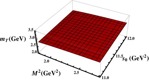
Figure 1: The mass $m_{T}$ of the tetraquark $T_{cs}^{0}$ as a function of the Borel and continuum threshold parameters.

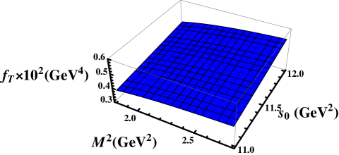
Figure 2: The same as in Fig. 1, but for the coupling $f_{T}$.

In Figs. 1 and 2 we plot the predictions for the mass $m_{T}$ and coupling $f_{T}$, in which one can see their dependence on the parameters $M^{2}$ and $s_{0}$.

Our results for the spectroscopic parameters of the tetraquark $T_{cs}^{0}$ read

$$m_{T} = \left(2878\pm 128\right)~{}\mathrm{MeV},\$$

$$f_{T} = \left(0.45\pm 0.08\right)\times 10^{-2}~{}\mathrm{GeV}^{4}.$$ (7)

These predictions will be used below to study the strong decays of $T_{cs}^{0}$.

II.2 Strong decays $T_{cs}^{0}\rightarrow D^{0}\overline{K}^{0}$ and $T_{cs}^{0}\rightarrow D^{+}K^{-}$

The spectroscopic parameters of the tetraquark $T_{cs}^{0}$ obtained in the previous subsection provide an information necessary to answer a question about its stability against the strong interactions. It is not difficult to see, that the mass $m_{T}$ makes kinematically allowed the strong decays $T_{cs}^{0}\rightarrow D^{0}\overline{K}^{0}$ and $T_{cs}^{0}\rightarrow D^{+}K^{-}$. There are other strong decay modes of $T_{cs}^{0}$, but these two channels are $S$-wave processes. Here, we are going to consider in a detailed form the channel $T_{cs}^{0}\rightarrow D^{0}\overline{K}^{0}$, and give final results for the second one.

The width of the decay $T_{cs}^{0}\rightarrow D^{0}\overline{K}^{0}$, apart from other parameters, is determined by the strong coupling $g_{TD^{0}\overline{K}^{0}}$ corresponding to the vertex $T_{cs}^{0}D^{0}\overline{K}^{0}$. Our aim is to calculate $g_{TD^{0}\overline{K}^{0}}$ which quantitatively describes strong interactions between the tetraquark and two conventional mesons. To this end, we use the LCSR method and begin from analysis of the correlation function

$$\Pi(p,q)=i\int d^{4}xe^{ipx}\langle\overline{K}^{0}(q)|\mathcal{T}\{J^{D^{0}}(x)J^{T\dagger}(0)\}|0\rangle,$$ (8)

where $J^{D^{0}}(x)$ is the interpolating current of the meson $D^{0}$; it has following form

$$J^{D^{0}}(x)(x)=\overline{u}(x)i\gamma_{5}c(x).$$ (9)

Standard recipes require to write $\Pi(p,q)$ in terms of physical parameters of the particles $T_{cs}^{0}$, $D^{0}$, and $\overline{K}^{0}$

$$\Pi^{\mathrm{Phys}}(p,q)=\frac{\langle 0|J^{D^{0}}|D^{0}(p)\rangle}{p^{2}-m_{D}^{2}}\langle D^{0}\left(p\right)\overline{K}^{0}(q)|T_{cs}^{0}(p^{\prime})\rangle$$

$$\times\frac{\langle T_{cs}^{0}(p^{\prime})|J^{T\dagger}|0\rangle}{p^{\prime 2}-m_{T}^{2}}+...,$$ (10)

where $p^{\prime}$ and $p$, $q$ are 4-momenta of the initial and final particles, respectively. In the expression above by dots we note contributions of excited resonances and continuum states. The correlation function $\Pi^{\mathrm{Phys}}(p,q)$ can be simplified by introducing the matrix elements

$$\langle 0|J^{D^{0}}|D^{0}(p)\rangle=\frac{f_{D}m_{D}^{2}}{m_{c}+m_{u}},$$

$$\langle D^{0}\left(p\right)\overline{K}^{0}(q)|T_{cs}^{0}(p^{\prime})\rangle=g_{TD^{0}\overline{K}^{0}}(p\cdot p^{\prime}).$$ (11)

The matrix element $\langle 0|J^{D^{0}}|D^{0}(p)\rangle$ is expressed in terms of $D^{0}$ meson’s mass $m_{D}$ and its decay constant $f_{D}$, whereas $\langle D^{0}\left(p\right)\overline{K}^{0}(q)|T_{cs}^{0}(p^{\prime})\rangle$ is written down using the strong coupling $g_{TD^{0}\overline{K}^{0}}$. In the soft-meson limit $q\rightarrow 0$ we get $p^{\prime}=p$ Agaev:2016dev , and must carry out the Borel transformation of $\Pi^{\mathrm{Phys}}(p,q=0)$ over the variable $p^{2}$, which gives

$$\mathcal{B}\Pi^{\mathrm{Phys}}(p^{2})=g_{TD^{0}\overline{K}^{0}}\frac{f_{D}m_{D}^{2}f_{T}m_{T}\widetilde{m}^{2}}{m_{c}+m_{u}}\frac{e^{-\widetilde{m}^{2}/M^{2}}}{M^{2}}\ldots,$$ (12)

where

$$\widetilde{m}^{2}=\frac{m_{T}^{2}+m_{D}^{2}}{2}.$$ (13)

The necessity to use the soft-meson approximation of the LCSR method and set $q=0$ is connected with features of tetraquark-meson-meson strong vertices. Because a tetraquark is built of four valence quarks, calculations of the correlation function (8) by contracting quark fields from relevant interpolating currents lead to appearance of two quark fields at the same space-time position, which, sandwiched between the vacuum and $\overline{K}^{0}$ meson, generate the local matrix elements of $\overline{K}^{0}$. Then, to preserve the 4-momentum conservation at the vertex one has to set $q=0$, and employ technical tools of soft-meson approach elaborated in the full LCSR method as the approximation to vertices containing only conventional mesons Belyaev:1994zk . Let us emphasize that in the case of tetraquark-meson-meson vertices soft limit is an only way to calculate corresponding strong couplings in the framework of the LCSR method.

The soft approximation modifies the physical side of the sum rules. A problem is that in the soft limit some of contributions arising from the higher resonances and continuum states even after the Borel transformation remain unsuppressed. These terms correspond to vertices containing excited states of involved particles, and contaminate the physical side of sum rules. Therefore, before performing the continuum subtraction in the final sum rule they should be delated by means of some manipulations. This problem can be solved by acting on the physical side of the sum rule by the operator Belyaev:1994zk ; Ioffe:1983ju

$$\mathcal{P}(M^{2},\widetilde{m}^{2})=\left(1-M^{2}\frac{d}{dM^{2}}\right)M^{2}e^{\widetilde{m}^{2}/M^{2}},$$ (14)

which keeps unchanged the ground-state term removing, at the same time, unsuppressed contributions. Naturally, the operator $\mathcal{P}(M^{2},\widetilde{m}^{2})$ has to be applied to the QCD side of the sum rule as well, which has to be calculated in the soft-meson approximation and expressed in terms of the $\overline{K^{0}}$ meson’s local matrix elements.

In the soft limit the correlation function $\Pi^{\mathrm{OPE}}(p)$ is determined by the expression

$$\Pi^{\mathrm{OPE}}(p)=i\int d^{4}xe^{ipx}\epsilon\widetilde{\epsilon}\left[\gamma_{5}\widetilde{S}_{c}^{ib}(x){}\gamma_{5}S_{u}^{di}(-x){}\gamma_{5}\right]_{\alpha\beta}$$

$$\times\langle\overline{K}^{0}|\overline{s}_{\alpha}^{c}(0)d_{\beta}^{e}(0)|0\rangle,$$ (15)

where

$$\widetilde{S}(x)=CS_{c(q)}^{T}(x)C.$$ (16)

In Eqs. (15) and (16), $S_{c(q)}(x)$ are the $c$ quark and light quark propagators explicit expressions of which can be found in Ref. Sundu:2018uyi ; for simplicity we do not provide these formulas here.

As is seen, the correlation function  $\Pi^{\mathrm{OPE}}(p)$ depends on local matrix elements $\langle\overline{K}^{0}|\overline{s}_{\alpha}^{c}(0)d_{\beta}^{e}(0)|0\rangle$, which should be recast to forms suitable for expressing them as standard matrix elements of $\overline{K}^{0}$. For these purposes, we employ the expansion

$$\overline{s}_{\alpha}^{c}d_{\beta}^{e}\rightarrow\frac{1}{12}\Gamma_{\beta\alpha}^{j}\delta^{ce}\left(\overline{s}\Gamma^{j}d\right),$$ (17)

where $\Gamma^{j}$ is the full set of Dirac matrices

$$\Gamma^{j}=\mathbf{1,\ }\gamma_{5},\ \gamma_{\lambda},\ i\gamma_{5}\gamma_{\lambda},\ \sigma_{\lambda\rho}/\sqrt{2}.$$ (18)

Then operators $\overline{s}\Gamma^{j}d$ and ones appeared due to $G$ insertions from propagators $\widetilde{S}$ and $S$, give rise to local matrix elements of the $\overline{K}^{0}$ meson. Substituting Eq. (17) into the correlation function and performing the color summation in accordance with prescriptions described in Ref. Agaev:2016dev , we fix twist-3 local matrix element of $\overline{K}^{0}$

$$\langle 0|\overline{d}(0)i\gamma_{5}s(0)|\overline{K}^{0}\rangle=\frac{f_{K^{0}}m_{K^{0}}^{2}}{m_{s}+m_{d}},$$ (19)

that contributes to the correlation function.

The function $\Pi^{\mathrm{OPE}}(p)$ contains the trivial Lorentz structure which is proportional to $I$. The Borel transformed and subtracted expression of the corresponding invariant amplitude $\Pi^{\mathrm{OPE}}(p^{2})$ reads

$$\Pi^{\mathrm{OPE}}(M^{2},s_{0})=\int_{(m_{c}+m_{s})^{2}}^{s_{0}}ds\rho^{\mathrm{pert.}}(s)e^{-s/M^{2}}$$

$$+\frac{\mu_{K^{0}}}{6}e^{-m_{c}^{2}/M^{2}}\left\{m_{c}\langle\overline{q}q\rangle+\frac{1}{8}\langle\frac{\alpha_{s}G^{2}}{\pi}\rangle\left[1+\frac{m_{c}^{2}}{6M^{2}}\right]\right.$$

$$-\frac{m_{c}^{3}}{4M^{4}}\langle\overline{s}g_{s}\sigma Gs\rangle-\frac{g_{s}^{2}m_{c}^{4}}{81M^{6}}\langle\overline{q}q\rangle^{2}$$

$$\left.-\frac{m_{c}\pi^{2}}{18M^{6}}\langle\frac{\alpha_{s}G^{2}}{\pi}\rangle\langle\overline{q}q\rangle\left(m_{c}^{2}-3M^{2}\right)\right\},$$ (20)

where

$$\rho^{\mathrm{pert.}}(s)=\frac{\mu_{K^{0}}}{24\pi^{2}}(3m_{c}^{2}-s),$$ (21)

and $\mu_{K^{0}}=f_{K^{0}}m_{K^{0}}^{2}/(m_{s}+m_{d})$. Let us note that calculations of $\Pi^{\mathrm{OPE}}(M^{2},s_{0})$ are carried out by taking into account nonperturbative terms up to seventh dimension. Then, the sum rule for the strong coupling $g_{TD^{0}\overline{K}^{0}}$ takes the form

$$g_{TD^{0}\overline{K}^{0}}=\frac{m_{c}+m_{u}}{f_{D}m_{D}^{2}f_{T}m_{T}\widetilde{m}^{2}}\mathcal{P}(M^{2},\widetilde{m}^{2})\Pi^{\mathrm{OPE}}(M^{2},s_{0}).$$ (22)

The width of the decay $T_{cs}^{0}\rightarrow D^{0}\overline{K}^{0}$ is given by the formula

$$\Gamma[T_{cs}^{0}\rightarrow D^{0}\overline{K}^{0}]=\frac{g_{TD^{0}\overline{K}^{0}}^{2}m_{D}^{2}}{8\pi}\lambda\left(1+\frac{\lambda^{2}}{m_{D}^{2}}\right),$$ (23)

where

$$\lambda = \lambda\left(m_{T}^{2},m_{D}^{2},m_{K^{0}}^{2}\right)=\frac{1}{2m_{T}}\left[m_{T}^{4}+m_{K^{0}}^{4}+m_{D}^{4}\right.$$ (24)

$$\left.-2(m_{T}^{2}m_{D}^{2}+m_{T}^{2}m_{K^{0}}^{2}+m_{K^{0}}^{2}m_{D}^{2})\right]^{1/2}.$$

In numerical computations of $g_{TD^{0}\overline{K}^{0}}$ the Borel and continuum threshold parameters are chosen as in Eq. (6). To visualize a sensitivity of the strong coupling on these parameters, in Fig. 3 we depict the dependence of $|g_{TD^{0}\overline{K}^{0}}|$ on $M^{2}$ and $s_{0}$; ambiguities generated by the choice of these parameters do not exceed  $\pm 19\%$ of the central value.

For the strong coupling $g_{TD^{0}\overline{K}^{0}}$ our analysis yields

$$|g_{TD^{0}\overline{K}^{0}}|=(0.37\pm 0.07)~{}\mathrm{GeV}^{-1}.$$ (25)

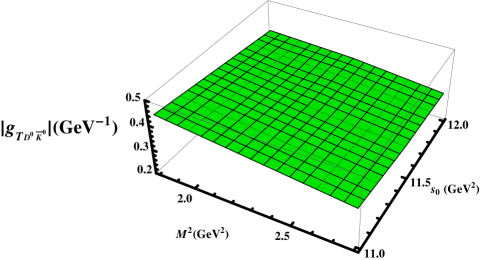
Figure 3: The strong coupling $|g_{TD^{0}\overline{K}^{0}}|$ as a function of the Borel and continuum threshold parameters.

Using the result obtained for $g_{TD^{0}\overline{K}^{0}}$, we can evaluate the partial width of the decay $T_{cs}^{0}\rightarrow D^{0}\overline{K}^{0}$:

$$\Gamma\left(T_{cs}^{0}\rightarrow D^{0}\overline{K}^{0}\right)=(15.35\pm 4.11)~{}\mathrm{MeV.}$$ (26)

The decay $T_{cs}^{0}\rightarrow D^{+}K^{-}$ can be analyzed by the same manner. The difference is connected with quark contents of the mesons $D^{+}$ and $K^{-}$ that generate small modifications, for example, $\widetilde{\Pi}^{\mathrm{OPE}}(p)$ takes the form

$$\widetilde{\Pi}^{\mathrm{OPE}}(p) = i\int d^{4}xe^{ipx}\epsilon\widetilde{\epsilon}\left[\gamma_{5}\widetilde{S}_{c}^{ib}(x){}\gamma_{5}S_{d}^{di}(-x){}\gamma_{5}\right]_{\alpha\beta}$$ (27)

$$\times\langle K^{-}|\overline{u}_{\alpha}^{c}(0)s_{\beta}^{e}(0)|0\rangle.$$

Therefore, we write down the final results for the strong coupling $g_{TD^{+}K^{-}}$ and corresponding decay width

$$|g_{TD^{+}K^{-}}|=(0.38\pm 0.06)\ \mathrm{GeV}^{-1},$$

$$\Gamma\left(T_{cs}^{0}\rightarrow D^{+}K^{-}\right)=(15.40\pm 3.44)~{}\mathrm{MeV}.$$ (28)

These dominant decay channels allow us to estimate the full width of the tetraquark $T_{cs}^{0}$

$$\Gamma=(30.8\pm 5.4)~{}\mathrm{MeV.}$$ (29)

In light of obtained prediction for the full width of $T_{cs}^{0}$, we classify it as a relatively narrow unstable tetraquark.

III Semileptonic decay $T_{bs}^{-}\rightarrow T_{cs}^{0}l\overline{\nu}_{l}$

The semileptonic decay $T_{bs}^{-}\rightarrow T_{cs}^{0}l\overline{\nu}_{l}$ runs through the transitions $b\rightarrow W^{-}c$ and $W^{-}\rightarrow l\overline{\nu_{l}}$. It is not difficult to see that decays with all lepton species $l=e,\ \mu$ and $\tau$ are kinematically allowed processes.

The transition $b\rightarrow c$ at the tree-level can be described using the effective Hamiltonian

$$\mathcal{H}^{\mathrm{eff}}=\frac{G_{F}}{\sqrt{2}}V_{bc}\overline{c}\gamma_{\mu}(1-\gamma_{5})b\overline{l}\gamma^{\mu}(1-\gamma_{5})\nu_{l},$$ (30)

where $G_{F}$ is the Fermi coupling constant, and $V_{bc}$ is the relevant Cabibbo-Kobayashi-Maskawa (CKM) matrix element. After placing the effective Hamiltonian $\mathcal{H}^{\mathrm{eff}}$ between the initial and final tetraquarks and factoring out the lepton fields one gets the matrix element of the current

$$J_{\mu}^{\mathrm{W}}=\overline{c}\gamma_{\mu}(1-\gamma_{5})b.$$ (31)

The matrix element $\langle T_{cs}^{0}(p^{\prime})|J_{\mu}^{\mathrm{W}}|T_{bs}^{-}(p)\rangle$ can be expressed in terms of the form factors $G_{i}(q^{2})$ that parameterize the long-distance dynamics of the weak transition. In the case of scalar tetraquarks it has the rather simple form

$$\langle T_{cs}^{0}(p^{\prime})|J_{\mu}^{\mathrm{W}}|T_{bs}^{-}(p)\rangle=G_{1}(q^{2})P_{\mu}+G_{2}(q^{2})q_{\mu},$$ (32)

where $p$ and $p^{\prime}$ are the momenta of the tetraquarks $T_{bs}^{-}$ and $T_{cs}^{0}$, respectively. Here, we use the shorthand notations $P_{\mu}=p_{\mu}^{\prime}+p_{\mu}$ and $q_{\mu}=p_{\mu}-p_{\mu}^{\prime}$. The $q_{\mu}$ is the momentum transferred to the leptons, and $q^{2}$ changes within the limits $m_{l}^{2}\leq q^{2}\leq(m-m_{T})^{2}$, where $m_{l}$ is the mass of a lepton $l$.

The sum rules for the form factors $G_{i}(q^{2}),i=1,2$ can be derived from the three-point correlation function

$$\Pi_{\mu}(p,p^{\prime}) = i^{2}\int d^{4}xd^{4}ye^{i(p^{\prime}y-px)}$$ (33)

$$\times\langle 0|\mathcal{T}\{J^{T}(y)J_{\mu}^{\mathrm{W}}(0)J^{\dagger}(x)\}|0\rangle,$$

where $J^{T}(y)$ and $J(x)$ are the interpolating currents for the states $T_{cs}^{0}$ and $T_{bs}^{-}$, respectively. The current $J^{T}(y)$ is given by Eq. (2), whereas for $J(x)$ we use the expression

$$J(x)=\epsilon\widetilde{\epsilon}[b_{b}^{T}(x)C\gamma_{5}s_{c}(x)][\overline{u}_{d}(x)\gamma_{5}C\overline{d}_{e}^{T}(x)].$$ (34)

First, we express the correlation function $\Pi_{\mu}(p,p^{\prime})$ in terms of the spectroscopic parameters of the tetraquark and mesons, and fix the physical side of the sum rule, i.e., find the function $\Pi_{\mu}^{\mathrm{Phys}}(p,p^{\prime})$. It can be easily written down in the form

$$\Pi_{\mu}^{\mathrm{Phys}}(p,p^{\prime})=\frac{\langle 0|J^{T}|T_{cs}^{0}(p^{\prime})\rangle\langle T_{cs}^{0}(p^{\prime})|J_{\mu}^{\mathrm{W}}|T_{bs}^{-}(p)\rangle}{(p^{2}-m^{2})(p^{\prime 2}-m_{T}^{2})}$$

$$\times\langle T_{bs}^{-}(p)|J^{\dagger}|0\rangle+\ldots,$$ (35)

where we take explicitly into account a contribution of the ground-state particles, and denote by dots effects due to excited and continuum states.

Using the tetraquarks’ matrix elements and expressing the vertex $\langle T(p^{\prime})|J_{\mu}^{\mathrm{W}}|T_{bs}^{-}(p)\rangle$ in terms of the weak transition form factors $G_{i}(q^{2})$ it is not difficult to find that

$$\Pi_{\mu}^{\mathrm{Phys}}(p,p^{\prime}) = \frac{f_{T}m_{T}fm}{(p^{2}-m^{2})(p^{\prime 2}-m_{T}^{2})}$$ (36)

$$\times\left[G_{1}(q^{2})P_{\mu}+G_{2}(q^{2})q_{\mu}\right],$$

where the matrix element of the state $T_{bs}^{-}$ is defined by

$$\langle T_{bs}^{-}(p)|J^{\dagger}|0\rangle=fm.$$ (37)

To calculate $\Pi_{\mu}(p,p^{\prime})$, we employ the interpolating currents and quark propagators, and find

$$\Pi_{\mu}^{\mathrm{OPE}}(p,p^{\prime})=i^{2}\int d^{4}xd^{4}ye^{i(p^{\prime}y-px)}\epsilon\widetilde{\epsilon}\epsilon^{\prime}\widetilde{\epsilon}^{\prime}$$

$$\times\mathrm{Tr}\left[\gamma_{5}\widetilde{S}_{d}^{e^{\prime}e}(x-y)\gamma_{5}S_{u}^{d^{\prime}d}(x-y)\right]\mathrm{Tr}\left[\gamma_{\mu}(1-\gamma_{5})\right.$$

$$\left.\times S_{b}^{ib}(-x)\gamma_{5}\widetilde{S}_{s}^{cc^{\prime}}(y-x)\gamma_{5}S_{c}^{b^{\prime}i}(y)\right].$$ (38)

Then, the sum rules for the form factors $G_{i}(q^{2})$ can be derived by equating the invariant amplitudes corresponding to the same Lorentz structures in $\Pi_{\mu}^{\mathrm{Phys}}(p,p^{\prime})$ and $\Pi_{\mu}^{\mathrm{OPE}}(p,p^{\prime})$. Afterwards, we carry out the double Borel transformation over $p^{\prime 2}$ and $p^{2}$ which is required to suppress contributions of the higher excited and continuum states, and perform the continuum subtraction. These operations lead to the sum rules

$$G_{i}(\mathbf{M}^{2},\mathbf{s}_{0},q^{2})=\frac{1}{f_{T}m_{T}fm}\int_{(m_{b}+m_{s})^{2}}^{s_{0}}ds$$

$$\times\int_{(m_{c}+m_{s})^{2}}^{s_{0}^{\prime}}ds^{\prime}\rho_{i}(s,s^{\prime},q^{2})e^{(m^{2}-s)/M_{1}^{2}}e^{(m_{T}^{2}-s^{\prime})/M_{2}^{2}},$$

(39)

where $\rho_{1(2)}(s,s^{\prime},q^{2})$ are the spectral densities calculated as the imaginary parts of the correlation function $\Pi_{\mu}^{\mathrm{OPE}}(p,p^{\prime})$ with dimension-five accuracy. In Eq. (39) $\mathbf{M}^{2}$ and $\mathbf{s}_{0}$ are a couple of the Borel and continuum threshold parameters, respectively; the set $(M_{1}^{2},s_{0})$ corresponds to the initial state $T_{bs}^{-}$, and the second set $(M_{2}^{2},s_{0}^{\prime})$ describes the tetraquark $T_{cs}^{0}$.

Parameters for numerical computations of $G_{i}(\mathbf{M}^{2},\mathbf{s}_{0},q^{2})$ are listed in Table 1. The mass and coupling of the tetraquark $T_{bs}^{-}$

$$m = (5380~{}\pm 170)~{}\mathrm{MeV},$$

$$f = (2.1\pm 0.5)\times 10^{-3}~{}\mathrm{GeV}^{4},$$ (40)

and working windows for the parameters $(M_{1}^{2},s_{0})$

$$M_{1}^{2}\in[3.4,\ 4.8]~{}\mathrm{GeV}^{2},\ s_{0}\in[35,\ 37]~{}\mathrm{GeV}^{2}$$ (41)

are borrowed from Ref. Sundu:2019feu . The regions for $(M_{2}^{2},s_{0}^{\prime})$ and spectroscopic parameters of $T_{cs}^{0}$ are given by Eqs. (6) and (7), respectively. In numerical computations we also use the Fermi coupling constant $G_{F}=1.16637\times 10^{-5}~{}\mathrm{GeV}^{-2}$ and CKM matrix element $|V_{bc}|=(41.2\pm 1.01)\times 10^{-3}$. Like all quantities extracted from sum rule computations, the weak form factors $G_{1(2)}(q^{2})$ depend on the Borel and continuum threshold parameters $\mathbf{M}^{2}$ and $\mathbf{s}_{0}.$ Ambiguities connected with the choice of $(\mathbf{M}^{2},\mathbf{s}_{0})$ and ones due to other input parameters form theoretical errors of the sum rule analysis, which will be taken into account in the fit functions.

To obtain the width of the decay $T_{bs}^{-}\rightarrow T_{cs}^{0}l\overline{\nu}_{l}$ one must integrate the differential decay rate $d\Gamma/dq^{2}$ (see, explanation below) of this process in the kinematical limits $m_{l}^{2}\leq q^{2}\leq(m-m_{T})^{2}$. In the interval $m_{l}^{2}\leq q^{2}\leq 5$ $\mathrm{GeV}^{2}$ the QCD sum rules lead to reliable predictions for the form factors $G_{i}(q^{2})$ , which do not cover the whole integration region $m_{l}^{2}\leq q^{2}\leq 6.26$ $\mathrm{GeV}^{2}$. Therefore, we replace the weak form factors $G_{i}(q^{2})$ by the fit functions $\mathcal{G}_{i}(q^{2})$, which at $q^{2}$ accessible for the sum rule computations coincide with $G_{i}(q^{2})$, but can be easily extrapolated to the full integration region.

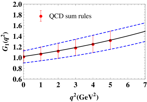
Figure 4: Dependence of the weak form factor $G_{1}(q^{2})$ on $q^{2}$: the QCD sum rule predictions and the fit function $\mathcal{G}_{1}(q^{2})$. The solid line corresponds to the central values of the parameters $\mathcal{G}_{1}^{0},\ g_{1}^{1},\ g_{2}^{1}$, for the upper dashed curve $\mathcal{G}_{1}^{0}=1.126,\ g_{1}^{1}=1.792,\ g_{2}^{1}=-0.875$, whereas for the lower dashed line $\mathcal{G}_{1}^{0}=0.901,\ g_{1}^{1}=1.255,\ g_{2}^{1}=1.106$.

Figure 5: The form factor $|G_{2}(q^{2})|$. The solid line describes the central function. Parameters of the upper and lower dashed curves are $\mathcal{G}_{1}^{0}=-0.982,\ g_{1}^{1}=1.771,\ g_{2}^{1}=-0.545$, and $\mathcal{G}_{1}^{0}=-0.790,\ g_{1}^{1}=1.039,\ g_{2}^{1}=2.414$, respectively.

For the fit functions we choose the following analytic expressions

$$\mathcal{G}_{i}(q^{2})=\mathcal{G}_{i}^{0}\exp\left[g_{1}^{i}\frac{q^{2}}{m^{2}}+g_{2}^{i}\left(\frac{q^{2}}{m^{2}}\right)^{2}\right].$$ (42)

In Figs. 4 and 5 one can see the QCD sum rule predictions for the form factors $G_{1}(q^{2})$ and $|G_{2}(q^{2})|$, in which ambiguities of computations are shown as error bars. Using the central values of the form factors and a standard fitting procedure, for the parameters of the functions $\mathcal{G}_{1}(q^{2})$ and $\mathcal{G}_{2}(q^{2})$ we get

$$\mathcal{G}_{1}^{0} = 1.022,\ g_{1}^{1}=1.383,\ g_{2}^{1}=0.756,$$

$$\mathcal{G}_{2}^{0} = -0.886,\ g_{1}^{2}=1.440,\ g_{2}^{2}=0.813.$$ (43)

The upper and lower limits of the sum rule results are employed to find corresponding extrapolating functions, plotted in the figures in the form of dashed curves. Various combinations of these functions are used to estimate theoretical errors of the semileptonic processes’ partial widths.

The differential decay rate $d\Gamma/dq^{2}$ of the process $T_{bs}^{-}\rightarrow T_{cs}^{0}l\overline{\nu}_{l}$ can be calculated using the expression derived in Ref. Sundu:2019feu , where one needs to replace parameters of the tetraquarks and weak form factors. Calculations yield the following predictions

$$\Gamma\left(T_{bs}^{-}\rightarrow T_{cs}^{0}e^{-}\overline{\nu}_{e}\right) = \left(1.55\pm 0.42\right)\times 10^{-10}\ \mathrm{MeV},$$

$$\Gamma\left(T_{bs}^{-}\rightarrow T_{cs}^{0}\mu^{-}\overline{\nu}_{\mu}\right) = \left(1.54\pm 0.42\right)\times 10^{-10}\ \mathrm{MeV},$$

$$\Gamma\left(T_{bs}^{-}\rightarrow T_{cs}^{0}\tau^{-}\overline{\nu}_{\tau}\right) = \left(1.91\pm 0.54\right)\times 10^{-11}\ \mathrm{MeV}.$$

Then, for the full width and mean lifetime of the tetraquark $T_{bs}^{-}$ we find

$$\Gamma_{\mathrm{full}} = \left(3.28\pm 0.60\right)\times 10^{-10}\ \mathrm{MeV},$$

$$\tau = 2.01_{-0.31}^{+0.44}\times 10^{-12}\ \text{{s}}.$$ (45)

Branching ratios of the processes $T_{bs}^{-}\rightarrow D^{0}\overline{K}^{0}l\overline{\nu}_{l}$ and $T_{bs}^{-}\rightarrow D^{+}K^{-}l\overline{\nu}_{l}$ can be found using $\mathcal{BR}\left(T_{bs}^{-}\rightarrow T_{cs}^{0}l\overline{\nu}_{l}\right)$ and $\mathcal{BR}\left(T_{cs}^{0}\rightarrow D^{0}\overline{K}^{0}\right)\simeq\mathcal{BR}\left(T_{cs}^{0}\rightarrow D^{+}K^{-}\right)\simeq 0.5$. Results of these computations are collected in Table 2.

Channels	$\mathcal{BR}$
$T_{bs}^{-}\to D^{0}\overline{K}^{0}e^{-}\overline{\nu}_{e}$	$0.24$
$T_{bs}^{-}\to D^{+}K^{-}e^{-}\overline{\nu}_{e}$	$0.24$
$T_{bs}^{-}\to D^{0}\overline{K}^{0}\mu^{-}\overline{\nu}_{\mu}$	$0.23$
$T_{bs}^{-}\to D^{+}K^{-}\mu^{-}\overline{\nu}_{\mu}$	$0.23$
$T_{bs}^{-}\to D^{0}\overline{K}^{0}\tau^{-}\overline{\nu}_{\tau}$	$0.03$
$T_{bs}^{-}\to D^{+}K^{-}\tau^{-}\overline{\nu}_{\tau}$	$0.03$
$T_{bb}^{-}\to D^{0}\overline{K}^{0}L$	$1.7\times 10^{-2}$
$T_{bb}^{-}\to D^{+}K^{-}L$	$1.6\times 10^{-2}$
$T_{bb}^{-}\to D^{0}\overline{K}^{0}\pi^{+}e^{-}e^{-}$	$9.8\times 10^{-3}$
$T_{bb}^{-}\to D^{0}\overline{K}^{0}K^{+}e^{-}e^{-}$	$1.3\times 10^{-3}$
$T_{bb}^{-}\to D^{+}K^{-}\pi^{+}e^{-}e^{-}$	$9.4\times 10^{-3}$
$T_{bb}^{-}\to D^{+}K^{-}K^{+}e^{-}e^{-}$	$1.3\times 10^{-3}$

Table 2: The decay channels of the tetraquarks $T_{bs}^{-}$ and $T_{bb}^{-}$, and their branching ratios. Above we have used $L=e^{-}e^{+}e^{-}$.

IV Analysis and conclusions

In the present work we have calculated width and mean lifetime of the tetraquark $T_{bs}^{-}$, which is stable against the strong and electromagnetic decays. To this end, we have computed partial widths of its dominant semileptonic decays $T_{bs}^{-}\rightarrow T_{cs}^{0}l\overline{\nu}_{l}$, where $l$ is one of $e,\ \mu$ and $\tau$ leptons. The tetraquark $T_{cs}^{0}$ appeared at the final state of this process is the strong-interaction unstable particle and decays to conventional mesons $D^{0}\overline{K}^{0}$ and $D^{+}K^{-}$. We have also evaluated the spectroscopic parameters of $T_{cs}^{0}$ and computed the partial widths of its strong decays, which allowed us to find the branching ratios of the processes $T_{bs}^{-}\rightarrow D^{0}\overline{K}^{0}l\overline{\nu}_{l}$ and $T_{bs}^{-}\rightarrow D^{+}K^{-}l\overline{\nu}_{l}$. Predictions for the mass of $T_{bs}^{-}$ obtained in our previous work Sundu:2019feu , and results for the full widths and mean lifetimes of the tetraquarks $T_{bs}^{-}$ and $T_{cs}^{0}$ provide a basis for their experimental investigations.

But, information gained in the present article is important also to trace back transformations of the state $T_{bb}^{-}$. Stable nature of the $T_{bb}^{-}$ was explored and confirmed by different methods and authors. This state transforms in accordance with the chains of decays $T_{bb}^{-}\rightarrow Z_{bc}^{0}l\bar{\nu_{l}}\rightarrow T_{bs}^{-}l\bar{\nu_{l}}\overline{l^{\prime}}\nu_{l^{\prime}}$ and $T_{bb}^{-}\rightarrow Z_{bc}^{0}l\bar{\nu_{l}}\rightarrow T_{bs}^{-}Pl\bar{\nu_{l}}$, where we take into account both the semileptonic and nonleptonic decays of the scalar tetraquark $Z_{bc}^{0}$ Sundu:2019feu . Now with information on decays of the tetraquark $T_{bs}^{-}$ at hands, we can fix some of decay channels of $T_{bb}^{-}$ to conventional mesons. It is not difficult to see, that $T_{bb}^{-}\rightarrow D^{0}\overline{K}^{0}l\bar{\nu_{l}}\overline{l^{\prime}}\nu_{l^{\prime}}l^{\prime\prime}\overline{\nu}_{l^{\prime\prime}}$, $T_{bb}^{-}\rightarrow D^{+}K^{-}l\bar{\nu_{l}}\overline{l^{\prime}}\nu_{l^{\prime}}l^{\prime\prime}\overline{\nu}_{l^{\prime\prime}}$, $T_{bb}^{-}\rightarrow D^{0}\overline{K}^{0}Pl\bar{\nu_{l}}l^{\prime\prime}\overline{\nu}_{l^{\prime\prime}}$, and $T_{bb}^{-}\rightarrow D^{+}K^{-}Pl\bar{\nu_{l}}l^{\prime\prime}\overline{\nu}_{l^{\prime\prime}}$ are among important modes of such transformations. In Fig. 6 we depict some of such channels, which at the second leg of weak transformations contain products of semileptonic and nonleptonic decays of $Z_{bc}^{0}$. Their branching ratios can be found using results of Refs. Agaev:2018khe ; Sundu:2019feu and information obtained in the present work. For the decay mode $T_{bb}^{-}\rightarrow D^{0}\overline{K}^{0}L$ these computations yield

$$\mathcal{BR}\left(T_{bb}^{-}\rightarrow D^{0}\overline{K}^{0}L\right) = \mathcal{BR}\left(T_{bb}^{-}\rightarrow T_{bs}^{-}e^{-}e^{+}\right)$$

$$\times\mathcal{BR}\left(T_{bs}^{-}\rightarrow D^{0}\overline{K}^{0}e^{-}\right) = 1.7\times 10^{-2}.$$ (46)

For simplicity, we have denoted $L=e^{-}e^{+}e^{-}$ and omitted final-state neutrinos. The branching ratios of other processes [shown in Fig. 6] are also collected in Table 2. The decay channels of $T_{bb}^{-}$ containing $\mu$ and $\tau$ leptons, and mixed modes with $e\mu$, $e\tau$, $\mu\tau$, and $e\mu\tau$ leptons at the final state can be analyzed by the same manner.

The results for the width and lifetime of the tetraquark $T_{bs}^{-}$, and predictions for branching ratios of $T_{bs}^{-}$ and $T_{bb}^{-}$ have been obtained using their dominant semileptonic decays. In the case of weak transformations of the tetraquark $T_{bb}^{-}$ we took into account the nonleptonic decays of the scalar state $Z_{bc}^{0}$.  During the present analysis we have neglected nonleptonic decay modes of $T_{bs}^{-}$ and $T_{bb}^{-}$. Our investigations show that branching ratios of nonleptonic channels are suppressed relative to semileptonic ones Sundu:2019feu ; Agaev:2019kkz , nevertheless, by including into consideration these modes one can refine the prediction (46) and ones presented in Table 2.

We also ignored subdominant decay channels which may be generated by weak decays of heavy quarks, and which are suppressed due to smallness of the relevant CKM matrix elements. At earlier levels of the weak cascade some of these modes might create unstable 4-quarks that dissociate to other than $D$ and $K$ mesons.

Finally, in the present work the exotic meson $T_{bs}^{-}$ has been treated as a scalar particle. But in the decay $Z_{bc}^{0}\rightarrow T_{bs}^{-}\overline{l}\nu_{l}$ the final-state tetraquark may bear also other quantum numbers. By including into analysis these options one may reveal new decay modes of $Z_{bc}^{0}$, and, hence of $T_{bb}^{-}$. Investigation of these alternative decays can add a valuable new information on features of the exotic mesons $T_{bb}^{-}$ and $T_{bs}^{-}$.

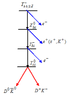
Figure 6: Some of the decay modes of the tetraquark $T_{bb;\overline{u}\overline{d}}^{-}$.

References

- (1) H. X. Chen, W. Chen, X. Liu and S. L. Zhu, Phys. Rept. 639, 1 (2016).
- (2) H. X. Chen, W. Chen, X. Liu, Y. R. Liu and S. L. Zhu, Rept. Prog. Phys. 80, 076201 (2017).
- (3) A. Esposito, A. Pilloni and A. D. Polosa, Phys. Rept. 668, 1 (2017).
- (4) A. Ali, J. S. Lange and S. Stone, Prog. Part. Nucl. Phys. 97, 123 (2017).
- (5) S. L. Olsen, T. Skwarnicki and D. Zieminska, Rev. Mod. Phys. 90, 015003 (2018).
- (6) J. P. Ader, J. M. Richard and P. Taxil, Phys. Rev. D 25, 2370 (1982).
- (7) H. J. Lipkin, Phys. Lett. B 172, 242 (1986).
- (8) S. Zouzou, B. Silvestre-Brac, C. Gignoux and J. M. Richard, Z. Phys. C 30, 457 (1986).
- (9) J. Carlson, L. Heller and J. A. Tjon, Phys. Rev. D 37, 744 (1988).
- (10) F. S. Navarra, M. Nielsen and S. H. Lee, Phys. Lett. B 649, 166 (2007).
- (11) M. Karliner and J. L. Rosner, Phys. Rev. Lett. 119, 202001 (2017).
- (12) E. J. Eichten and C. Quigg, Phys. Rev. Lett. 119, 202002 (2017).
- (13) S. S. Agaev, K. Azizi, B. Barsbay and H. Sundu, Phys. Rev. D 99, 033002 (2019).
- (14) H. Sundu, S. S. Agaev and K. Azizi, Eur. Phys. J. C 79, 753 (2019).
- (15) S. S. Agaev, K. Azizi and H. Sundu, arXiv:1905.07591 [hep-ph].
- (16) S. S. Agaev, K. Azizi and H. Sundu, Phys. Rev. D 99, 114016 (2019).
- (17) G.-Q. Feng, X.-H. Guo and B.-S. Zou, arXiv:1309.7813 [hep-ph].
- (18) A. Francis, R. J. Hudspith, R. Lewis, and K. Maltman, Phys. Rev. D 99, 054505 (2019)
- (19) T. F. Caramees, J. Vijande, and A. Valcarce, Phys. Rev. D 99, 014006 (2019).
- (20) M. A. Shifman, A. I. Vainshtein and V. I. Zakharov, Nucl. Phys. B 147, 385 (1979).
- (21) M. A. Shifman, A. I. Vainshtein and V. I. Zakharov, Nucl. Phys. B 147, 448 (1979).
- (22) R. M. Albuquerque, J. M. Dias, K. P. Khemchandani, A. Martinez Torres, F. S. Navarra, M. Nielsen and C. M. Zanetti, J. Phys. G 46, 093002 (2019).
- (23) I. I. Balitsky, V. M. Braun and A. V. Kolesnichenko, Nucl. Phys. B 312, 509 (1989).
- (24) V. M. Belyaev, V. M. Braun, A. Khodjamirian and R. Ruckl, Phys. Rev. D 51, 6177 (1995).
- (25) R. L. Jaffe, Phys. Rept. 409, 1 (2005).
- (26) S. S. Agaev, K. Azizi and H. Sundu, Phys. Rev. D 93, 074002 (2016).
- (27) S. S. Agaev, K. Azizi and H. Sundu, Phys. Rev. D 93, 114007 (2016).
- (28) H. Sundu, S. S. Agaev and K. Azizi, Phys. Rev. D 97, 054001 (2018).
- (29) H. Sundu, S. S. Agaev and K. Azizi, Eur. Phys. J. C 79, 215 (2019).
- (30) B. L. Ioffe and A. V. Smilga, Nucl. Phys. B 232, 109 (1984).
- (31) H. Sundu, B. Barsbay, S. S. Agaev and K. Azizi, Eur. Phys. J. A 54, 124 (2018).