Faraday patterns generated by Rabi oscillation in a binary Bose-Einstein condensate

Abstract

The interaction between atoms in a two-component Bose-Einstein condensate (BEC) is effectively modulated by the Rabi oscillation. This periodic modulation of the effective interaction is shown to generate Faraday patterns through parametric resonance. We show that there are multiple resonances arising from the density and spin waves in a two-component BEC, and investigate the interplay between the Faraday-pattern formation and the phase separation.

I Introduction

Bose-Einstein condensates (BECs) of ultracold alkali atoms are generated through magnetic and optical means, and are created in one of several hyperfine states of the electronic ground state. When the hyperfine state is coherently coupled with another hyperfine state by microwave or radio-frequency wave, Rabi oscillation occurs between the two states, resulting in a two-component (binary) BEC Matthews ; Nicklas ; Hamner . Coherently-coupled two-component BECs have much richer physics than single-component BECs, and they have been studied in detail theoretically Williams ; Park ; Kasamatsu ; Lee ; Sabbatini ; Dror ; Bernier ; Fialko ; Usui .

Recently, a coherently-coupled BEC of the hyperfine states $|F=1,m_{1}\rangle$ and $|F=1,m_{2}\rangle$ of ${}^{87}{\rm Rb}$ atoms was experimentally investigated Shibata , where $F$ is the hyperfine spin and $m_{1,2}=0,\pm 1$ are the magnetic quantum numbers. Since $F=1$ is the lowest-energy hyperfine spin, stable Rabi oscillation over a long duration was realized with precise control of the coupling field. In this experiment, excitation patterns were observed in the atomic cloud after Rabi oscillation with a small Rabi frequency ($\sim 100$ Hz), which was also confirmed numerically (Figs. 7(d) and 8 in Ref. Shibata ). This excitation of the BEC can be interpreted as follows. Suppose that all the atoms are in state 1 or 2 at some instant. The energy density of the interatomic interaction for this state is $g_{11}n^{2}/2$ or $g_{22}n^{2}/2$, where $n$ is the atomic density and $g_{ij}$ is the interaction coefficient between states $i$ and $j$. When states 1 and 2 become equally populated in the course of the Rabi oscillation, the energy density becomes $(g_{11}+2g_{12}+g_{22})n^{2}/8$. Thus, the interatomic interaction effectively oscillates in time due to the Rabi oscillation unless $g_{11}=g_{22}=g_{12}$. Such an effective modulation of the interaction can be used to control the dynamics of BECs Saito07 ; Eto .

In a single-component BEC, the periodic modulation of the interaction by, e.g., a Feshbach resonance, was shown to excite a pattern in the atomic density through a parametric resonance, which is called the Faraday pattern Staliunas . Such Faraday-pattern formation was experimentally observed by periodic modulation of the transverse confinement in a cigar-shaped BEC Engels , which effectively modulates the interaction. The Faraday waves can also be generated in two-component BECs Balaz , dipolar BECs Lakomy , and Fermi-Bose mixtures Abdullaev .

Motivated by the experiment reported in Ref. Shibata , in the present paper we theoretically investigate Faraday-pattern formation in a coherently-coupled two-component BEC. Based on the oscillation of the effective interaction due to the Rabi oscillation, Faraday patterns are shown to be excited without any modulation of external parameters. Since there are two types of elementary excitations in a two-component BEC, i.e., density and spin waves, multiple wave-number excitations appear in the Faraday waves. In the case of $g_{11}=g_{22}$, we find that three wave numbers are excited, which arises from the resonance of the Rabi oscillation with density-density, density-spin, and spin-spin waves. We show using Floquet analysis that the Faraday-wave excitation can coexist with phase separation due to the immiscibility of the two components.

The reminder of this paper is organized as follows. Section II formulates the mean-field description of a coherently-coupled two-component BEC. Section III presents numerical results of the time evolution of the system. Section IV performs the Floquet analysis of the Rabi induced excitations. Section V studies the resonance conditions and provides the mechanism of multiple resonances, and Sec. VI concludes the study.

II Coupled Gross-Pitaevskii equations

We consider a two-component BEC in uniform space at zero temperature. In the mean-field approximation, the condensate is described by the macroscopic wave functions $\psi_{1}(\bm{r},t)$ and $\psi_{2}(\bm{r},t)$ for components 1 and 2, respectively. We normalize the length, time, and atomic density by an arbitrary length $L$, time $T$, and density $n_{0}$, where $\hbar T=ML^{2}$ is satisfied with $M$ being the mass of an atom. The coupled Gross-Pitaevskii (GP) equations are then given by

$$i\frac{\partial\psi_{1}}{\partial t} = -\frac{\nabla^{2}}{2}\psi_{1}+g_{11}|\psi_{1}|^{2}\psi_{1}+g_{12}|\psi_{2}|^{2}\psi_{1}-i\Omega\psi_{2},$$

$$i\frac{\partial\psi_{2}}{\partial t} = -\frac{\nabla^{2}}{2}\psi_{2}+g_{22}|\psi_{2}|^{2}\psi_{2}+g_{12}|\psi_{1}|^{2}\psi_{2}+i\Omega^{*}\psi_{1},$$

where $g_{ij}=4\pi a_{ij}L^{2}n_{0}$ is the nondimensional interaction coefficient and $a_{ij}$ is the scattering length between atoms in states $i$ and $j$. The phase of the Rabi coupling is determined by the phase of the coupling field, and $\Omega$ is taken to be real and positive without loss of generality. In the following study, for simplicity, we assume $g_{11}=g_{22}\equiv g>0$ and $g_{12}>0$. We also assume that the initial state is the uniform state with equal population, $\psi_{1}(t=0)=\psi_{2}(t=0)=1/\sqrt{2}$.

In the noninteracting system ($g=g_{12}=0$), the uniform solution of Eq. (1) is given by

$$\psi_{1}(t) = \cos(\Omega t+\pi/4),$$ (2a)

$$\psi_{2}(t) = \sin(\Omega t+\pi/4).$$ (2b)

We note that the oscillation frequency of the densities $|\psi_{1}|^{2}$ and $|\psi_{2}|^{2}$ is $2\Omega$.

In the absence of the Rabi coupling ($\Omega=0$), the miscibility of the two components is determined by the interaction coefficients $g_{ij}$. The frequency $\omega$ of the excitation with wave number $k$ for the state $\psi_{1}=\psi_{2}=1/\sqrt{2}$ has the form Pethick ,

$$\omega^{2} = \frac{\epsilon_{k}}{2}\left[2\epsilon_{k}+g_{11}+g_{22}\pm\sqrt{(g_{11}-g_{22})^{2}+4g_{12}^{2}}\right]$$ (3)

$$= \epsilon_{k}(\epsilon_{k}+g\pm g_{12}),$$

where $\epsilon_{k}=k^{2}/2$ is the kinetic energy of a free particle. The frequency $\omega$ in Eq. (3) becomes imaginary for $g_{11}g_{22}=g^{2}<g_{12}^{2}$, which corresponds to the instability of phase separation. The most unstable wave number is $k=\sqrt{g_{12}-g}$.

When the Rabi coupling $\Omega$ is much larger than the energy scale of the interaction $g_{ij}$, the system is effectively described by the dressed states $\psi_{\pm}=(\psi_{1}\pm\psi_{2})/\sqrt{2}$. The intra- and inter-component interactions for the dressed states are given by Nicklas ; Search ; Jenkins ; Merhasin

$$g_{++}=g_{--} = \frac{1}{4}(g_{11}+g_{22}+2g_{12})=\frac{1}{2}(g+g_{12}),$$ (4a)

$$g_{+-} = \frac{1}{2}(g_{11}+g_{22})=g.$$ (4b)

Using these effective interaction coefficients $g_{++}$, $g_{--}$, and $g_{+-}$ in Eq. (3) instead of $g_{11}$, $g_{22}$, and $g_{12}$, we find

$$\omega^{2}=\epsilon_{k}[\epsilon_{k}+(3g+g_{12})/2],\;\epsilon_{k}[\epsilon_{k}+(g_{12}-g)/2].$$ (5)

The miscibility condition for large $\Omega$ is therefore opposite to that for $\Omega=0$, i.e., the uniformly mixed state $\psi_{1}=\psi_{2}=1/\sqrt{2}$ is unstable and phase separation occurs for $g>g_{12}$. The most unstable wave number is $k=\sqrt{(g-g_{12})/2}$.

III Time evolution of the system

We investigate the dynamics of the system by solving the GP equation (1) numerically. For simplicity, we consider a two-dimensional (2D) system. In the numerical calculation, the wave function is discretized into a $2048\times 2048$ mesh, where each mesh has dimensions $dx=dy=0.2$, and the size of the entire 2D space is $409.6\times 409.6$. The time evolution is obtained using the pseudospectral method recipe . The initial state of $\psi_{1}(\bm{r})$ and $\psi_{2}(\bm{r})$ is set to be a constant $1/\sqrt{2}$ plus a small random number for each mesh. This small initial noise breaks the exact numerical symmetry and triggers spatial pattern formation. Because the pseudospectral method is used, a periodic boundary condition is imposed.

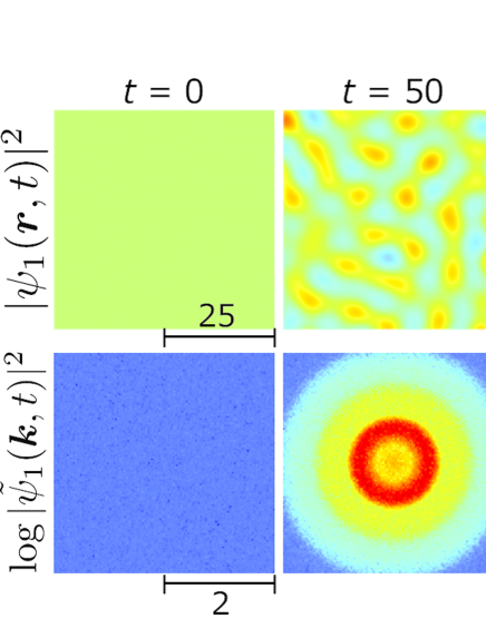
Figure 1: (color online) Time evolution of the system without Rabi coupling ($\Omega=0$) for the immiscible condition, $g=1$ and $g_{12}=1.4$. The density profile of component 1 in the real space, $|\psi_{1}(\bm{r},t)|^{2}$, and that in the momentum space, $\log|\tilde{\psi}_{1}(\bm{k},t)|^{2}$, are shown in the upper and lower panels, respectively. See the Supplemental Material for a movie illustrating the dynamics movies .

First, in Fig. 1, we show the case without Rabi coupling ($\Omega=0$), where the interaction coefficients satisfy the immiscible condition, $g=1$ and $g_{12}=1.4$. We see that the density pattern emerges in $|\psi_{1}(\bm{r},t)|^{2}$ (and also in $|\psi_{2}(\bm{r},t)|^{2}$) at $t=50$, which leads to the phase separation at $t=70$. In this dynamics, the total density $|\psi_{1}(\bm{r},t)|^{2}+|\psi_{2}(\bm{r},t)|^{2}$ is almost constant with time. In Fig. 1, the logarithmic density profile in the momentum space, $\log|\tilde{\psi}_{1}(\bm{k},t)|^{2}$, is also shown, where

$$\tilde{\psi}_{j}(\bm{k},t)=\sum_{\bm{r}}\psi_{j}(\bm{r},t)e^{-i\bm{k}\cdot\bm{r}}$$ (6)

is the discrete Fourier transformation over the numerical mesh. The ring-shaped peak appears in the momentum distribution due to the pattern formation. The radius of the ring at $t=50$ is $k\simeq 0.4$-$0.8$, which includes the most unstable wave number predicted from Eq. (3), $k=\sqrt{g_{12}-g}\simeq 0.63$.

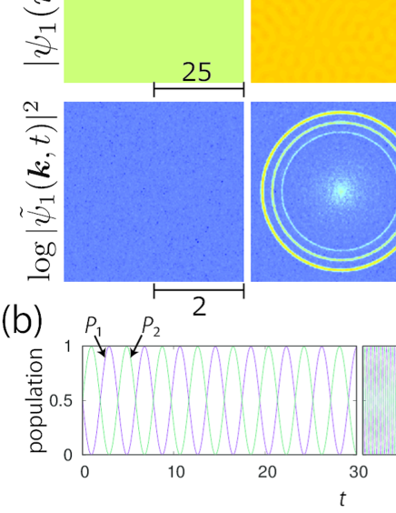
Figure 2: (color online) Time evolution of the system with Rabi coupling ($\Omega=0.8$) for $g=1$ and $g_{12}=1.4$. (a) The density profile of component 1 in the real space, $|\psi_{1}(\bm{r},t)|^{2}$, and that in the momentum space, $\log|\tilde{\psi}_{1}(\bm{k},t)|^{2}$, are shown in the upper and lower panels, respectively. See the Supplemental Material for a movie illustrating the dynamics movies . (b) Time evolution of the population $P_{j}(t)$ in each component for $0<t<30$ and $30<t<300$.

Figure 2 shows the dynamics in the presence of the Rabi coupling with $\Omega=0.8$. Starting from $\psi_{1}=\psi_{2}=1/\sqrt{2}$, the two components undergo Rabi oscillation with angular frequency $\omega\simeq 1.62$, as shown in Fig. 2(b). Due to the Rabi oscillation, the lifetime of the uniform distribution is prolonged, compared with that in Fig. 1 for the same interaction coefficients $g=1$ and $g_{12}=1.4$. At $t\simeq 100$, the density pattern emerges, as shown in Fig. 2(a). Interestingly, three rings appear in the momentum space at $t\simeq 100$ (i.e., three wave numbers are simultaneously excited) with radii $k\simeq 1.3$, $1.5$, and $1.75$. Among the three rings, the outermost ring becomes dominant and the innermost ring disappears at $t\simeq 143$. In Fig. 2(b), the time evolution of the population $(j=1,2)$

$$P_{j}(t)=\frac{\int|\psi_{j}(\bm{r},t)|^{2}d\bm{r}}{\int\left[|\psi_{1}(\bm{r},t)|^{2}+|\psi_{2}(\bm{r},t)|^{2}\right]d\bm{r}}$$ (7)

of each component is plotted. The amplitude of the oscillation in $P_{j}(t)$ decreases as the pattern develops, which is due to the inhomogeneous Rabi oscillation.

In the following sections, we will show that the excitation of the three wave numbers in Fig. 2(a) is due to the interplay between the Rabi oscillation and the interatomic interaction. The population of each component oscillates due to the Rabi oscillation, and this leads to oscillation of the interaction energy because $g\neq g_{12}$. Such oscillation of the effective interaction causes parametric resonance with Bogoliubov modes, which is reminiscent of Faraday-pattern formation in a single-component BEC with time-dependent interaction Staliunas .

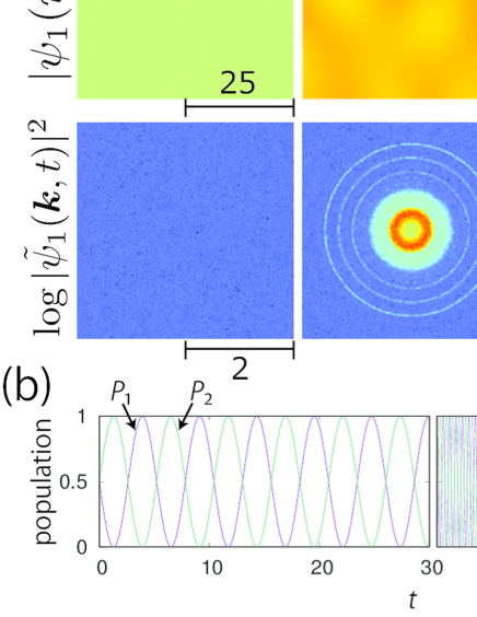
Figure 3: (color online) Time evolution of the system for $\Omega=0.6$, $g=1$, and $g_{12}=0.8$. (a) The density profile of component 1 in the real space, $|\psi_{1}(\bm{r},t)|^{2}$, and that in the momentum space, $\log|\tilde{\psi}_{1}(\bm{k},t)|^{2}$, are shown in the upper and lower panels, respectively. See the Supplemental Material for a movie illustrating the dynamics movies . (b) Time evolution of the population $P_{j}(t)$ in each component for $0<t<30$ and $30<t<300$.

Figure 3 shows the case of $g=1$ and $g_{12}=0.8$, for which the two components are miscible for $\Omega=0$ and immiscible for $\Omega\rightarrow\infty$. For the intermediate value of $\Omega$, the immiscibility coexists with the Faraday-pattern formation due to the Rabi oscillation. At $t\simeq 180$, a thick ring is observed near the center in the momentum space, in addition to the thin three rings. The central ring in the momentum space arises from the phase separation of the dressed states. According to Eq. (5), the most unstable wave number for $\Omega\rightarrow\infty$ is $k=\sqrt{(g-g_{12})/2}\simeq 0.3$, which is in reasonable agreement with the radius of the central ring. As shown later, the outer three rings correspond to the Faraday-like excitation due to the Rabi oscillation. In Figs. 2 and 3, the patterns also appear in component 2 (data not shown), and the total density $|\psi_{1}(\bm{r},t)|^{2}+|\psi_{2}(\bm{r},t)|^{2}$ is almost uniform.

IV Floquet analysis

To study the excitation spectra shown in Figs. 1-3 in more detail, we performed Floquet analysis as follows. The Rabi oscillation in the uniform system is described by the wave functions as ($j=1,2$)

$$\psi_{j}(t)=e^{-i\mu t}f_{j}(t),$$ (8)

where $\mu$ is a real constant and $f_{j}(t)$ are periodic complex functions satisfying $f_{j}(t+T)=f_{j}(t)$, with $T$ being the Rabi oscillation period. We write the small excitation of the state (8) as

$$\psi_{j}(\bm{r},t)=e^{-i\mu t}\left[f_{j}(t)+\delta\psi_{j}(\bm{r},t)\right].$$ (9)

We assume that the excitation has wave number $\bm{k}$,

$$\delta\psi_{j}(\bm{r},t)=u_{j}(t)e^{i\bm{k}\cdot\bm{r}}+v_{j}^{*}(t)e^{-i\bm{k}\cdot\bm{r}}.$$ (10)

Substituting Eqs. (9) and (10) into the GP equation (1), we obtain four coupled differential equations,

$$i\dot{u}_{1} = \left(\epsilon_{k}-\mu\right)u_{1}+g\left(2|f_{1}|^{2}u_{1}+f_{1}^{2}v_{1}\right)$$ (11a)

$$+g_{12}\left(|f_{2}|^{2}u_{1}+f_{1}f_{2}^{*}u_{2}+f_{1}f_{2}v_{2}\right)-i\Omega u_{2},$$

$$i\dot{v}_{1} = -\left(\epsilon_{k}-\mu\right)v_{1}-g\left(2|f_{1}|^{2}v_{1}+f_{1}^{*2}u_{1}\right)$$ (11b)

$$-g_{12}\left(|f_{2}|^{2}v_{1}+f_{1}^{*}f_{2}v_{2}+f_{1}^{*}f_{2}^{*}u_{2}\right)-i\Omega v_{2},$$

$$i\dot{u}_{2} = \left(\epsilon_{k}-\mu\right)u_{2}+g\left(2|f_{2}|^{2}u_{2}+f_{2}^{2}v_{2}\right)$$ (11c)

$$+g_{12}\left(|f_{1}|^{2}u_{2}+f_{1}^{*}f_{2}u_{1}+f_{1}f_{2}v_{1}\right)+i\Omega u_{1},$$

$$i\dot{v}_{2} = -\left(\epsilon_{k}-\mu\right)v_{2}-g\left(2|f_{2}|^{2}v_{2}+f_{2}^{*2}u_{2}\right)$$ (11d)

$$-g_{12}\left(|f_{1}|^{2}v_{2}+f_{1}f_{2}^{*}v_{1}+f_{1}^{*}f_{2}^{*}u_{1}\right)+i\Omega v_{1}.$$

The coefficients of $u_{j}(t)$ and $v_{j}(t)$ on the right-hand side of these equations are all periodic with period $T$, since $f_{1}(t)$ and $f_{2}(t)$ are periodic functions. Therefore, according to the Floquet theorem, there exist solutions $\bm{u}=(u_{1},v_{1},u_{2},v_{2})^{\rm tr}$ satisfying

$$\bm{u}(t)=e^{\lambda t}\bm{p}(t),$$ (12)

where tr indicates transpose, $\lambda$ is the Floquet exponent, and $\bm{p}(t)$ are periodic functions with period $T$. At $t=T$, Eq. (12) becomes

$$\bm{u}(T)=e^{\lambda T}\bm{p}(T)=e^{\lambda T}\bm{p}(0).$$ (13)

We perform the Floquet analysis numerically as follows. We first obtain the uniform solution (8) by solving the uniform GP equation using the Runge-Kutta method, which yields $\mu$, $T$, and $f_{j}(t)$. Next, we integrate Eq. (11) from $t=0$ to $t=T$ using the Runge-Kutta method, where the initial values of $\bm{u}$ are $\bm{u}_{a}(0)=(1,0,0,0)^{\rm tr}$, $\bm{u}_{b}(0)=(0,1,0,0)^{\rm tr}$, $\bm{u}_{c}(0)=(0,0,1,0)^{\rm tr}$, and $\bm{u}_{d}(0)=(0,0,0,1)^{\rm tr}$, giving $\bm{u}_{a}(T)$, $\bm{u}_{b}(T)$, $\bm{u}_{c}(T)$, and $\bm{u}_{d}(T)$, respectively. Using these results, we define a $4\times 4$ matrix as

$$U_{T}=[\bm{u}_{a}(T),\bm{u}_{b}(T),\bm{u}_{c}(T),\bm{u}_{d}(T)].$$ (14)

The values of $\bm{u}(t=T)$ for arbitrary initial values $\bm{u}(t=0)$ can be expressed as

$$\bm{u}(T)=U_{T}\bm{u}(0).$$ (15)

The eigenvalues and eigenvectors of $U_{T}$ thus correspond to $e^{\lambda T}$ and $\bm{p}(0)$ in Eq. (13), respectively.

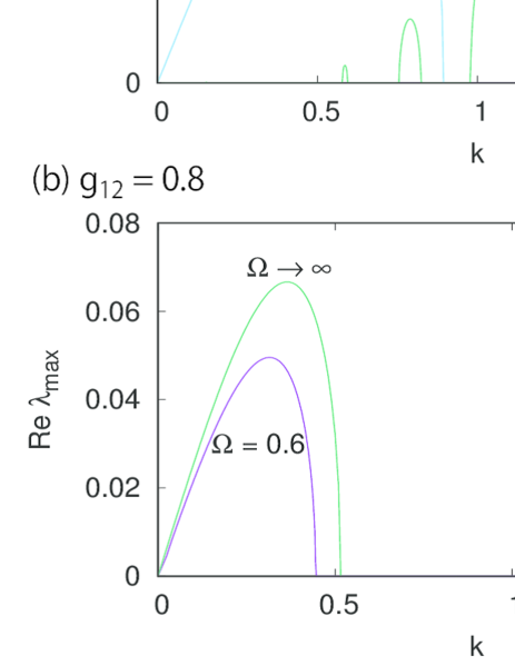
Figure 4: (color online) Largest real part of the Floquet exponent, ${\rm Re}\lambda_{\rm max}$, as a function of wave number $k$, obtained by solving Eq. (11) and diagonalizing Eq. (14) numerically. When ${\rm Re}\lambda_{\rm max}>0$, the system is dynamically unstable to excitation of wave number $k$. (a) $g_{12}=1.4$ and (b) $g_{12}=0.8$. In (a) and (b), we plot the imaginary part of $\omega$ in Eqs. (3) and (5) for $\Omega\rightarrow 0$ and $\Omega\rightarrow\infty$, respectively. The vertical dotted lines are the solutions of Eq. (22).

We focus on the largest real part of the Floquet exponents $\lambda$ among the four eigenvalues of $U_{T}$, which we denote ${\rm Re}\lambda_{\rm max}$. If ${\rm Re}\lambda_{\rm max}$ is positive, $\bm{u}(t)$ (and therefore $\delta\psi(\bm{r},t)$) grows exponentially in time, and the uniform state is unstable to excitation of wave numbers $k$. Figure 4 shows ${\rm Re}\lambda_{\rm max}$ as a function of wave number $k$. In Fig. 4(a), the three peaks for $\Omega=0.8$ correspond to the three rings in Fig. 2. The three wave numbers in Figs. 2 and 4(a) agree well. As the Rabi coupling $\Omega$ is decreased, the peaks shift toward smaller $k$ and the rightmost peak grows while the left two peaks decay, as shown by the curve for $\Omega=0.3$ in Fig. 4(a). In the limit of $\Omega\rightarrow 0$, the left two peaks disappear and the rightmost peak converges to the imaginary part of $\omega$ in Eq. (3). Thus, for $g_{12}>g$, the instability of Faraday-wave excitation due to the Rabi oscillation for $\Omega\neq 0$ is continuously connected to the phase separation for $\Omega=0$.

In the case of $g_{12}=0.8$, the uniform state $\psi_{1}=\psi_{2}=1/\sqrt{2}$ is stable in the absence of the Rabi coupling, and therefore, ${\rm Re}\lambda_{\rm max}=0$ for $\Omega=0$. In the limit of $\Omega\rightarrow\infty$, on the other hand, the dressed states become immiscible according to Eq. (4). In Fig. 4(b), we plot the imaginary part of $\omega$ in Eq. (5). For an intermediate value of $\Omega$, in addition to the dressed-state instability, the three peaks appear, as shown by the curve of $\Omega=0.6$ in Fig. 4(b). Thus, in this parameter regime, the phase-separation instability of the dressed states coexists with the instability of Faraday-wave excitation due to the Rabi oscillation. In the case of $g_{12}=g=1$, we find that ${\rm Re}\lambda_{\rm max}=0$ for any $\Omega$, i.e., the uniform state is stable.

V Resonance condition

In Figs 2, 3, and 4, we numerically found that three wave numbers are excited by the Rabi oscillation. Here, we clarify the mechanism of this excitation spectrum.

First we consider the case of $g=g_{12}$. For the initial condition $\psi_{1}(0)=\psi_{2}(0)=1/\sqrt{2}$, the uniform solution of the GP equation (1) is given by

$$\psi_{1}(t) = e^{-igt}\cos(\Omega t+\pi/4),$$ (16a)

$$\psi_{2}(t) = e^{-igt}\sin(\Omega t+\pi/4).$$ (16b)

We add a small excitation to this state as

$$\psi_{1}(\bm{r},t) = e^{-igt}\left[\cos(\Omega t+\pi/4)+\delta\psi_{1}(\bm{r},t)\right],$$ (17a)

$$\psi_{2}(\bm{r},t) = e^{-igt}\left[\sin(\Omega t+\pi/4)+\delta\psi_{2}(\bm{r},t)\right].$$ (17b)

It is convenient to define $\delta\psi_{d}(\bm{r},t)$ and $\delta\psi_{s}(\bm{r},t)$ using $\delta\psi_{1}(\bm{r},t)$ and $\delta\psi_{2}(\bm{r},t)$ as

$$\delta\psi_{d} = \cos(\Omega t+\pi/4)\delta\psi_{1}+\sin(\Omega t+\pi/4)\delta\psi_{2},$$ (18a)

$$\delta\psi_{s} = \cos(\Omega t+\pi/4)\delta\psi_{2}-\sin(\Omega t+\pi/4)\delta\psi_{1}.$$ (18b)

Substituting Eqs. (17) and (18) into the GP equation (1) and neglecting the second- and third-order terms of $\delta\psi_{d}(\bm{r},t)$ and $\delta\psi_{s}(\bm{r},t)$, we obtain the linearized equations of motion for $\delta\psi_{d}(\bm{r},t)$ and $\delta\psi_{s}(\bm{r},t)$ as

$$i\frac{\partial\delta\psi_{d}}{\partial t} = -\frac{\nabla^{2}}{2}\delta\psi_{d}+g(\delta\psi_{d}+\delta\psi_{d}^{*}),$$ (19a)

$$i\frac{\partial\delta\psi_{s}}{\partial t} = -\frac{\nabla^{2}}{2}\delta\psi_{s}.$$ (19b)

Equation (19a) has the same form as that of the single-component BEC and thus gives the well-known Bogoliubov spectrum $\omega=\sqrt{\epsilon_{k}(\epsilon_{k}+2g)}$. This excitation modulates the total density, and can be regarded as a density wave. Equation (19b) gives the free-particle spectrum $\omega=\epsilon_{k}$. Since the interaction coefficient $g$ is not included in Eq. (19b), the excitation occurs with the total density kept constant, which can be regarded as the spin wave in the quasi-spin picture of two components. Since $\Omega$ is not included in both Eqs. (19a) and (19b), the Rabi oscillation has nothing to do with the excitations for $g=g_{12}$.

We next consider the case of $g\neq g_{12}$. We assume that the difference between $g$ and $g_{12}$ is much smaller than $\Omega$ and take the lowest order of

$$g_{12}-g\equiv\gamma$$ (20)

in the calculation. The corrections to the linearized equations of motion (19) then become (see Appendix)

$$i\frac{\partial\delta\psi_{d}}{\partial t} = -\frac{\nabla^{2}}{2}\delta\psi_{d}+g(\delta\psi_{d}+\delta\psi_{d}^{*})+\gamma A(\delta\psi_{d},\delta\psi_{s})$$

$$+\gamma B(\delta\psi_{d},\delta\psi_{s})\cos 4\Omega t+\gamma C(\delta\psi_{d},\delta\psi_{s})\sin 4\Omega t,$$

$$i\frac{\partial\delta\psi_{s}}{\partial t} = -\frac{\nabla^{2}}{2}\delta\psi_{s}+\gamma A^{\prime}(\delta\psi_{d},\delta\psi_{s})$$

$$+\gamma B^{\prime}(\delta\psi_{d},\delta\psi_{s})\cos 4\Omega t+\gamma C^{\prime}(\delta\psi_{d},\delta\psi_{s})\sin 4\Omega t.$$

The functions $A$, $A^{\prime}$, $B$, $B^{\prime}$, $C$, and $C^{\prime}$ in Eq. (21) are linear with respect to $\delta\psi_{d}$, $\delta\psi_{d}^{*}$, $\delta\psi_{s}$, and $\delta\psi_{s}^{*}$, whose explicit forms are given in Eq. (25) in the Appendix.

In the simple parametric resonance Landau , the resonance condition is determined by two frequencies: the natural frequency of the oscillator $\omega_{0}$ and the frequency of the external driving force $\omega_{1}$. The parametric resonance occurs when $\omega_{1}\simeq 2\omega_{0}=\omega_{0}+\omega_{0}$, where we neglect the higher-order resonance. In Eq. (21), the frequency of the driving force $\omega_{1}$ corresponds to the frequency $4\Omega$ of the sinusoidal functions, $\sin 4\Omega t$ and $\cos 4\Omega t$. The natural frequency of the oscillator $\omega_{0}$ corresponds to the frequencies that are determined by the first lines in Eq. (21), i.e., the terms without the sinusoidal functions. These frequencies $\omega_{d}$ and $\omega_{s}$ are obtained in Eq. (27) in the Appendix. The frequencies $\omega_{d}$ and $\omega_{s}$ in Eq. (27) reduce to $\omega_{d}\rightarrow\sqrt{\epsilon_{k}(\epsilon_{k}+2g)}$ and $\omega_{s}\rightarrow\epsilon_{k}$, for $\gamma\rightarrow 0$, and therefore, can be regarded as the excitation frequencies of the density and spin waves, respectively. Since there are two frequencies $\omega_{d}$ and $\omega_{s}$, the parametric resonance can occur for

$$4\Omega = 2\omega_{d},$$ (22a)

$$4\Omega = 2\omega_{s},$$ (22b)

$$4\Omega = \omega_{d}+\omega_{s}.$$ (22c)

For example, the resonance condition in Eq. (22c) can be understood as follows. In the dynamics of Eq. (21), $\delta\psi_{d}$ and $\delta\psi_{s}$ acquire a frequency component of $\omega_{d}$ ($\omega_{s}$). This frequency component is multiplied by the sinusoidal functions on the right-hand side of Eq. (21), which gives a frequency component of $4\Omega-\omega_{d}$ ($4\Omega-\omega_{s}$). The resonance occurs when this frequency is close to another frequency component of $\delta\psi_{d}$ and $\delta\psi_{s}$, i.e., $\omega_{s}$ ($\omega_{d}$), which gives Eq. (22c).

In Figs. 4(a) and 4(b), the three vertical dotted lines show the wave numbers obtained by solving Eq. (22) with respect to $k$ using Eq. (27). These analytically obtained wave numbers are in good agreement with the three numerically obtained peaks. The leftmost, middle, and rightmost peaks correspond to the resonance conditions in Eqs. (22a), (22c), and (22b), respectively. It is interesting to note that the rightmost peak is related to the spin-waves, because it continuously changes into the peak of $\Omega=0$ in Fig. 4(a). This is understood from the fact that the phase separation is triggered by the spin-wave excitation for $\Omega=0$.

We have thus shown that the excitations of multiple wave numbers observed in Figs 2, 3, and 4 originate from the parametric resonance of the density and spin waves with Rabi oscillation. The three wave numbers come from the combinations of density-density, spin-spin, and density-spin waves.

VI Conclusions

We investigated the dynamics of a two-component BEC with Rabi coupling, and found that the spatial patterns are excited by the Rabi oscillation. Due to the Rabi oscillation, the population of each component oscillates, resulting in the oscillation of the effective interaction. The oscillation of the interaction causes Faraday-pattern formation through parametric resonance. Since there are two kinds of excitations in a two-component BEC, i.e., density and spin waves, multiple resonances exist. We found three resonance peaks in the momentum space (Figs. 2, 3, and 4), which originate from the resonance of the Rabi oscillation with spin-spin, spin-density, and density-density wave excitations. We also showed that these parametric resonances coexist with the phase separation of the dressed states (Figs. 3 and 4(b)).

Experimentally, the multiple wave-number excitation presented in this paper may be observed by time-of-flight expansion with Bragg spectroscopy Vogels . The effects of trapping potential and the imbalance in the intracomponent interaction ($g_{11}\neq g_{22}$) deserve further study.

Appendix A Corrections to the equations of motion for excitations

In this appendix, we derive Eq. (21), which is the equation of motion for excitations in the case of $|\gamma|=|g_{12}-g|\ll\Omega$. We first make a correction to the uniform solution for $g=g_{12}$ in Eq. (16) as

$$\psi_{1}(t) = e^{-i(g+\delta\mu)t}\cos(\Omega t+\pi/4)[1+\Delta_{1}(t)],$$ (23a)

$$\psi_{2}(t) = e^{-i(g+\delta\mu)t}\sin(\Omega t+\pi/4)[1+\Delta_{2}(t)],$$ (23b)

where $\Delta_{1}$, $\Delta_{2}$, and $\delta\mu$ are $O(\gamma)$. Substituting Eq. (23) into the GP equation (1) and neglecting the terms of $O(\gamma^{2})$, we find $\delta\mu=\gamma/4$ and $\Delta_{1}=-\Delta_{2}=\gamma/(8\Omega)\cos 2\Omega t$.

We then add small excitations to the uniform wave functions as

$$\psi_{1}(\bm{r},t) = e^{-i(g+\gamma/4)t}\biggl{[}\cos(\Omega t+\pi/4)$$ (24a)

$$\times\left(1+\frac{i\gamma}{8\Omega}\cos 2\Omega t+\delta\psi_{1}(\bm{r},t)\right)\biggr{]},$$

$$\psi_{2}(\bm{r},t) = e^{-i(g+\gamma/4)t}\biggl{[}\sin(\Omega t+\pi/4)$$ (24b)

$$\times\left(1-\frac{i\gamma}{8\Omega}\cos 2\Omega t+\delta\psi_{2}(\bm{r},t)\right)\biggr{]}.$$

We substitute these wave functions into the GP equation (1) and neglect the terms of $O(\gamma^{2})$. After a straightforward calculation, we obtain

$$i\frac{\partial\delta\psi_{d}}{\partial t} = -\frac{\nabla^{2}}{2}\delta\psi_{d}+g(\delta\psi_{d}+\delta\psi_{d}^{*})$$ (25a)

$$+\frac{\gamma}{16}\biggl{\{}4(\delta\psi_{d}+\delta\psi_{d}^{*})+\frac{ig}{\Omega}(\delta\psi_{s}-\delta\psi_{s}^{*})$$

$$+\left[4(2\delta\psi_{d}+\delta\psi_{d}^{*})+\frac{ig}{\Omega}(\delta\psi_{s}-\delta\psi_{s}^{*})\right]\cos 4\Omega t$$

$$-\left[\frac{2ig}{\Omega}\delta\psi_{d}^{*}+4(2\delta\psi_{s}+\delta\psi_{s}^{*})\right]\sin 4\Omega t\biggr{\}},$$

$$i\frac{\partial\delta\psi_{s}}{\partial t} = -\frac{\nabla^{2}}{2}\delta\psi_{s}$$ (25b)

$$+\frac{\gamma}{16}\biggl{\{}-\frac{ig}{\Omega}(\delta\psi_{d}+\delta\psi_{d}^{*})+4(\delta\psi_{s}-\delta\psi_{s}^{*})$$

$$-\left[\frac{ig}{\Omega}(\delta\psi_{d}+\delta\psi_{d}^{*})+4(2\delta\psi_{s}+\delta\psi_{s}^{*})\right]\cos 4\Omega t$$

$$-4(2\delta\psi_{d}+\delta\psi_{d}^{*})\sin 4\Omega t\biggr{\}},$$

These equations of motion reduce to Eq. (19) for $\gamma=0$.

If we take the first and second lines in Eqs. (25a) and (25b), i.e., if we drop the terms with sinusoidal functions, the Bogoliubov matrix becomes

$$\left(\begin{array}[]{cccc}\epsilon_{k}+g+\frac{\gamma}{4}&g+\frac{\gamma}{4}&\frac{ig\gamma}{16\Omega}&\frac{ig\gamma}{16\Omega}\\ -g-\frac{\gamma}{4}&-\epsilon_{k}-g-\frac{\gamma}{4}&\frac{ig\gamma}{16\Omega}&\frac{ig\gamma}{16\Omega}\\ -\frac{ig\gamma}{16\Omega}&-\frac{ig\gamma}{16\Omega}&\epsilon_{k}+\frac{\gamma}{4}&-\frac{\gamma}{4}\\ -\frac{ig\gamma}{16\Omega}&-\frac{ig\gamma}{16\Omega}&\frac{\gamma}{4}&-\epsilon_{k}-\frac{\gamma}{4}\end{array}\right).$$ (26)

The eigenvalues of this matrix give the excitation spectrum, and are obtained as

$$\omega_{d} = \sqrt{\epsilon_{k}(\epsilon_{k}+2g)}+\frac{\epsilon_{k}\gamma}{4\sqrt{\epsilon_{k}(\epsilon_{k}+2g)}}+O(\gamma^{2}),$$ (27a)

$$\omega_{s} = \epsilon_{k}+\frac{\gamma}{4}+O(\gamma^{2}).$$ (27b)

These excitation frequencies reduce to $\omega_{d}=\sqrt{\epsilon_{k}(\epsilon_{k}+2g)}$ and $\omega_{s}=\epsilon_{k}$ for $\gamma=0$.

References

• (1) M. R. Matthews, B. P. Anderson, P. C. Haljan, D. S. Hall, M. J. Holland, J. E. Williams, C. E. Wieman, and E. A. Cornell, Watching a superfluid untwist itself: recurrence of Rabi oscillations in a Bose-Einstein condensate, Phys. Rev. Lett. 83, 3358 (1999).
• (2) E. Nicklas, H. Strobel, T. Zibold, C. Gross, B. A. Malomed, P. G. Kevrekidis, and M. K. Oberthaler, Rabi flopping induces spatial demixing dynamics, Phys. Rev. Lett. 107, 193001 (2011).
• (3) C. Hamner, Y. Zhang, J. J. Chang, C. Zhang, and P. Engels, Phase winding a two-component Bose-Einstein condensate in an elongated trap: experimental observation of moving magnetic orders and dark-bright solitons, Phys. Rev. Lett. 111, 264101 (2013).
• (4) J. Williams, R. Walser, J. Cooper, E. A. Cornell, and M. Holland, Excitation of a dipole topological state in a strongly coupled two-component Bose-Einstein condensate, Phys. Rev. A 61, 033612 (2000).
• (5) Q.-H. Park and J. H. Eberly, Nontopological vortex in a two-component Bose-Einstein condensate, Phys. Rev. A 70, 021602(R) (2004).
• (6) K. Kasamatsu, M. Tsubota, and M. Ueda, Vortex molecules in coherently coupled two-component Bose-Einstein condensate, Phys. Rev. Lett. 93, 250406 (2004).
• (7) C. Lee, Universality and anomalous mean-field breakdown of symmetry-breaking transitions in a coupled two-component Bose-Einstein condensate, Phys. Rev. Lett. 102, 070401 (2009).
• (8) J. Sabbatini, W. H. Zurek, and M. J. Davis, Phase separation and pattern formation in a binary Bose-Einstein condensate, Phys. Rev. Lett. 107, 230402 (2011).
• (9) N. Dror, B. A. Malomed, and J. Zend, Domain walls and vortices in linearly coupled systems, Phys. Rev. E 84, 046602 (2011).
• (10) N. R. Bernier, E. G. Dalla Torre, and E. Demler, Unstable avoided crossing in coupled spinor condensates, Phys. Rev. Lett. 113, 065303 (2014).
• (11) O. Fialko, B. Opanchuk, A. I. Sidorov, P. D. Drummond, and J. Brand, Fate of the false vacuum: Towards realization with ultra-cold atoms, Europhys. Lett. 110, 56001 (2015).
• (12) A. Usui and H. Takeuchi, Rabi-coupled countersuperflow in binary Bose-Einstein condensates, Phys. Rev. A 91, 063635 (2015).
• (13) K. Shibata, A. Torii, H. Shibayama, Y. Eto, H. Saito, and T. Hirano, Interaction modulation in a long-lived Bose-Einstein condensate by rf coupling, Phys. Rev. A 99, 013622 (2019).
• (14) H. Saito, R. G. Hulet, and M. Ueda, Stabilization of a Bose-Einstein droplet by hyperfine Rabi oscillations, Phys. Rev. A 76, 053619 (2007).
• (15) Y. Eto, M. Takahashi, M. Kunimi, H. Saito, and T. Hirano, Nonequilibrium dynamics induced by miscible-immiscible transition in binary Bose-Einstein condensates, New J. Phys. 18, 073029 (2016).
• (16) K. Staliunas, S. Longhi, and G. J. de Valcárcel, Faraday patterns in Bose-Einstein condensates, Phys. Rev. Lett. 89, 210406 (2002).
• (17) P. Engels, C. Atherton, and M. A. Hoefer, Observation of Faraday waves in a Bose-Einstein condensate, Phys. Rev. Lett. 98, 095301 (2007).
• (18) A. Balaž and A. I. Nicolin, Faraday waves in binary nonmiscible Bose-Einstein condensates, Phys. Rev. A 85, 023613 (2012).
• (19) K. Łakomy, R. Nath, and L Santos, Faraday patterns in coupled one-dimensional dipolar condensates, Phys. Rev. A 86, 023620 (2012).
• (20) F. Kh. Abdullaev, M. Ögren, and M. P. Sørensen, Faraday waves in quasi-one-dimensional superfluid Fermi-Bose mixtures, Phys. Rev. A 87, 023616 (2013).
• (21) See, e.g., C. J. Pethick and H. Smith, Bose-Einstein condensation in dilute gases, 2nd ed. (Cambridge Univ. Press, Cambridge, 2008).
• (22) C. P. Search and P. R. Berman, Manipulating the speed of sound in a two-component Bose-Einstein condensate, Phys. Rev. A 63, 043612 (2001).
• (23) S. D. Jenkins and T. A. B. Kennedy, Dynamic stability of dressed condensate mixtures, Phys. Rev. A 68, 053607 (2003).
• (24) I. M. Merhasin, B. A. Malomed, and R. Driben, Transition to miscibility in a binary Bose-Einstein condensate induced by linear coupling, J. Phys. B 38, 877 (2005).
• (25) W. H. Press, S. A. Teukolsky, W. T. Vetterling, and B. P. Flannery, Numerical Recieps, 3rd ed. (Cambridge Univ. Press, Cambridge, 2007).
• (26) See Supplemental Material at http://link.aps.org/supplemental/… for movies of the dynamics.
• (27) For example, L. D. Landau and E. M. Lifshitz, Mechanics (Pergamon, Oxford, 1960).
• (28) J. M. Vogels, K. Xu, C. Raman, J. R. Abo-Shaeer, and W. Ketterle, Experimental observation of the Bogoliubov transformation for a Bose-Einstein condensed gas, Phys. Rev. Lett. 88, 060402 (2002).