Effects of setting temperatures in the parallel tempering Monte Carlo algorithm

Abstract

Parallel tempering Monte Carlo has proven to be an efficient method in optimization and sampling applications. Having an optimized temperature set enhances the efficiency of the algorithm through more-frequent replica visits to the temperature limits. The approaches for finding an optimal temperature set can be divided into two main categories. The methods of the first category distribute the replicas such that the swapping ratio between neighboring replicas is constant and independent of the temperature values. The second-category techniques including the feedback-optimized method, on the other hand, aim for a temperature distribution that has higher density at simulation bottlenecks, resulting in temperature-dependent replica-exchange probabilities. In this paper, we compare the performance of various temperature setting methods on both sparse and fully connected spin-glass problems as well as fully connected Wishart problems that have planted solutions. These include two classes of problems that have either continuous or discontinuous phase transitions in the order parameter. Our results demonstrate that there is no performance advantage for the methods that promote nonuniform swapping probabilities on spin-glass problems where the order parameter has a smooth transition between phases at the critical temperature. However, on Wishart problems that have a first-order phase transition at low temperatures, the feedback-optimized method exhibits a time-to-solution speedup of at least a factor of two over the other approaches.

I Introduction

The parallel tempering (PT) Monte Carlo algorithm—also known as replica-exchange Monte Carlo Geyer (1991)—has been used effectively in solving a wide range of problems in various fields, such as physics, materials science, chemistry, logistics, and engineering Swendsen and Wang (1986); Hukushima and Nemoto (1996); Earl and Deem (2005); Katzgraber (2009). More recently, it has been repurposed as an effective heuristic for solving hard optimization problems  Moreno et al. (2003); Mandrà et al. (2016); Zhu et al. (2016). In fact, the winning entry of the 2016 MaxSAT competition used PT Monte Carlo as the underlying algorithmic engine of its optimization heuristic. While the method is extremely powerful, a careful tuning of the parameters is needed to ensure optimal run times Rathore et al. (2005); Hamze et al. (2010). In this work, we discuss the effects of setting the temperature values for the algorithm on paradigmatic spin-glass problems to elucidate which temperature setting approach is best suited for a particular problem type.

The PT algorithm simulates $M$ replicas of the original system at different temperatures, with periodic exchanges based on a Metropolis criterion between neighboring temperatures. Replica-exchange moves allow replicas to perform a random walk in temperature space, thereby efficiently overcoming energy barriers. Replicas at high temperatures improve algorithmic mixing, whereas replicas at low temperatures can reach equilibrium on a shorter time scale compared to typical simulations at a fixed low temperature Kofke (2004); Predescu et al. (2005); Fiore (2008); Machta (2009); Machta and Ellis (2011). The performance of the PT algorithm, like other MC simulation techniques, is highly dependent on its parameters, including the distribution of replicas in temperature space.

The approaches for setting the temperature values can be divided into two categories. The first category contains techniques that aim to distribute the replicas such that the probability of swapping adjacent replicas is independent of the temperature values, is equal across all adjacent pairs of replicas, and is sufficiently high so as to ensure frequent exchanges. The commonly used geometric distribution is considered to be a good approximation for temperature sets if the specific heat of the system is roughly constant Predescu et al. (2004). Other examples include the iterative methods presented by Hukushima and Nemoto Hukushima and Nemoto (1996) and Hukushima Hukushima (1999). In the former method, the acceptance ratios are measured using short MC runs, and the nearby inverse temperatures are iteratively placed farther or closer if their corresponding acceptance ratio is higher or lower than the average acceptance ratio, respectively. In the latter approach, referred to as the energy method, short MC runs are used to estimate the average energy as a function of the inverse temperature for deriving constant probabilities across replicas.

The second category comprises approaches that discard the premise of the first category that an independent and constant swapping ratio maximizes the extent to which replicas mix. The key idea of the approaches in the second category is to increase the performance of the algorithm by minimizing the round-trip time between the extremal temperatures for each replica. This translates to identifying the bottlenecks through measuring the local diffusivity of the replica ensemble and successively arranging temperature values closer to the bottlenecks of the simulation Trebst et al. (2004); Katzgraber et al. (2006). To our knowledge, there is no study in the literature that provides insights into the characteristics of problem types that can benefit most from the approaches in the second category, particularly when using PT as an optimization heuristic.

In this paper, we compare the performance of different approaches to determine the distribution of the replicas in the PT algorithm using both sparse and fully connected spin-glass problems, as well as fully connected Wishart problems that have planted solutions Hamze et al. (2019).

The paper is organized as follows. In Sec. II, we provide an overview of temperature setting methods. We introduce our benchmarking problems in Sec. III, followed by a presentation and discussion of the results in Sec. IV. Sec. V concludes the paper.

II Methods

In the PT algorithm, $M$ independent replicas of the system are simultaneously simulated at different temperature values $T_{1},T_{2},\ldots,T_{M}$. After performing a fixed number of MC sweeps at each temperature, swap moves between neighboring temperatures, $T_{i-1}$ and $T_{i}$, are proposed and accepted with probability

$$\mathbbm{P}(E_{i-1},T_{i-1}\leftrightarrow E_{i},T_{i})=\min(1,e^{\Delta\beta\Delta E}),$$

where $\Delta\beta=1/T_{i}-1/T_{i-1}$ and $\Delta E=E_{i}-E_{i-1}$.

As a result of the replica-exchange moves, replicas with high-energy states tend to be moved to high temperatures for diversification and the replicas with low-energy states tend to be moved to low temperatures for refinements. Although the simulation of $M$ replicas takes $M$ times more CPU time, the PT algorithm often has a faster time to solution and better scaling when compared to the simulated annealing algorithm Wang et al. (2015).

In this section, we describe four methods used in the literature to set the temperatures for each replica of the PT algorithm.

II.1 The feedback-optimized method

The goal of the feedback-optimized method is to find a temperature set ${T_{i}}$ such that the average round-trip time between two extremal temperatures is minimized Katzgraber et al. (2006). The primary concept of the feedback-optimized method is similar to that of the adaptive algorithm presented in the context of ensemble optimization Trebst et al. (2004), where the local diffusivity is measured to identify the bottlenecks in a feedback loop, after which the temperatures are placed near the simulation bottlenecks.

To measure the rate at which a replica visits a given temperature, a label of either “up” or “down” is assigned to the replica when it first visits the lowest ($T_{1}$) or the highest ($T_{\mbox{\scriptsize{M}}}$) temperature. The label of the replica does not change until its first visit to the opposite temperature extreme. As illustrated in Fig. 1, the label of replica $i$ is initially set to “none,” changes to “down” on its first visit to the highest temperature, remains unchanged until the replica reaches the lowest temperature, and is then set to “up.” We define $n_{\mbox{\scriptsize{up}}}(T_{i})$ and $n_{\mbox{\scriptsize{down}}}(T_{i})$ as the number of replicas with labels “up” and “down,” respectively, that visit temperature $T_{i}$ during the simulation. The fraction of replicas that have recently visited the lowest temperature before visiting $T_{i}$ is given below. We refer to $f(T_{i})$ as “flow” in this paper, given by

$$f(T_{i}) =\frac{n_{\mbox{\scriptsize{up}}}(T_{i})}{n_{\mbox{\scriptsize{up}}}(T_{i})+n_{\mbox{\scriptsize{down}}}(T_{i})}$$

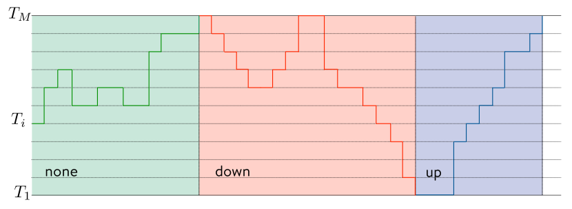
Figure 1: An example of replica $i$’s trajectory during the simulation. Its label is initially set to “none,” changes to “down” on visiting the highest temperature, and remains unchanged before hitting the lowest temperature, at which point it is set to “up.”

Following Fick’s law of diffusion, which states that the net rate of particles moving through an area equals the gradient times the diffusion constant Atkins and De Paula (2006), the rate $j$ at which a replica visits a given temperature $T$ can be stated as

$$j =D(T)\eta(T)\frac{df}{dT},$$ (1)

where $D(T)$ is the local diffusivity and $\eta(T)$ is the probability density function for replicas visiting temperature $T$. Defining the round-trip time $\tau=\frac{1}{j}$, we have

$$\tau=\frac{1}{D(T)\eta(T)\frac{df}{dT}}.$$

Rearranging the above expression yields the following:

$$\tau\int_{T}\frac{df}{dT}dT=\int_{T}\frac{1}{D(T)\eta(T)}dT.$$

Since $\int_{T}\frac{df}{dT}dT=1$, we have

$$\tau=\int_{T}\frac{1}{D(T)\eta(T)}dT.$$

To find a temperature set that minimizes the round-trip time subject to a proper probability distribution of replicas, the feedback-optimized method solves the following optimization problem:

$$\min_{\begin{subarray}{c}T\end{subarray}}\int_{T}\frac{1}{D(T)\eta(T)}dT$$

$$\mbox{s.t.}\int_{T}\eta(T)dT=1.$$

Defining the Lagrange function as

$$\mathcal{L}(T,\lambda)=\int_{T}\frac{1}{D(T)\eta(T)}dT-\lambda\big{[}\int_{T}\eta(T)dT-1\big{]},$$

we have

$$\frac{\partial{\mathcal{L}}}{\partial T}=\frac{1}{D(T)\eta(T)}-\lambda\eta(T)=0,$$

which results in

$$\eta(T)=\frac{1}{\sqrt{\lambda D(T)}}.$$ (2)

The solution of the Lagrange function shows that at the optimal temperature set, the optimal density function $\eta(T)$ is proportional to the inverse square root of the diffusion constant. Following the assumption that $\eta(T)=C/\Delta T$ in Ref. Katzgraber et al. (2006) and based on Eq. (1), we can further show how to estimate the probability density function by measuring the flow as

$$\frac{1}{D(T)}\propto\frac{\frac{df}{dT}}{\Delta T}\,,$$ (3)

and substituting it in Eq. (2) gives the following:

$$\eta(T)\propto{\sqrt{\frac{\frac{df}{dT}}{\Delta T}}}.$$

It can be also shown that

$$j =D(T)\eta(T)\frac{df}{dT}$$

$$=\frac{1}{\lambda\eta^{2}(T)}\eta(T)\frac{df}{dT}\longrightarrow\eta(T)\propto\frac{df}{dT}\propto\frac{1}{\Delta T},$$

which implies that at the optimal temperature set, the flow has a constant decay, that is, $f(T_{i})-f(T_{i+1})=1/(M-1)$, where $M$ is the number of replicas. We refer to this flow as the “optimal flow” where the flow at replica $i~{}(i=1,\ldots,M)$ equals $1-(i-1)/(M-1)$.

To find the optimal temperature set in practice, we follow the iterative steps presented in Algorithm 1 which is based on the algorithm discussed in Ref. Katzgraber et al. (2006), but with some modifications. The purpose of the algorithm is to find the temperature values by first measuring the flow values and then estimating the probability distribution until convergence.

Algorithm 1   Feedback-Optimized Method

1:initialize an arbitrary temperature set $\{T_{1},\ldots,T_{i},\ldots,T_{M}\}$ in ascending order and set the number of repeats $n=1$.

2:repeat

3:    perform the PT simulation and measure the flow vector $\{f(T_{i})\}$.

4:    smooth the flow vector.

5:    estimate the probability density function

$$\eta(T_{i})=C\sqrt{\frac{f(T_{i})-f(T_{i+1})}{T_{i+1}-T_{i}}}.$$

6:    find $C$ to ensure that

$$\int_{T_{1}}^{T_{M}}\eta(T)dT=1.$$

7:    find the new temperature ${T_{i}}$ such that

$$\int_{T_{1}}^{T_{i}}\eta(T)dT=\frac{i-1}{M-1}.$$

8:until $n=n_{\scriptsize{\mbox{max}}}$

To smooth the flow vector, we first filter out the flow value of replica $i$ if it is not within $\pm\epsilon~{}(0.5)$ of the optimal flow value $f^{*}_{i}=1-(i-1)/(M-1)$. More specifically, we remove $f(T_{i})$ from the flow vector and $T_{i}$ from the temperature vector if $f(T_{i})\notin[f^{*}_{i}-\epsilon,f^{*}_{i}+\epsilon]$. We then interpolate the flow as a monotonic function of temperature using the remaining flow and temperature values based on the method presented in Ref. Steffen (1990). Denoting the interpolated function as $g$, the flow of replica $i$ with temperature $T_{i}$, $f(T_{i})$, is then updated to $g(T_{i})$ before proceeding to the next step in the algorithm.

Repeating the core procedure of Algorithm 1 $n_{\scriptsize{\mbox{max}}}$ times, each with a large number of sweeps, the final temperature vector will be the one that has the lowest $L^{2}$-norm distance from the optimal flow vector.

II.2 The energy method

Hukushima Hukushima (1999) proposed a method that is simpler than the feedback-optimized method for determining the temperature values of the parallel tempering replicas. The scheme starts from an initial arbitrary temperature distribution, fixes the extremal temperatures, and iteratively adjusts the intermediate temperatures such that the replica-exchange probability for all adjacent temperatures is equal. Since this scheme is based on estimating the energy at each replica as a function of its inverse temperature, we refer to the method as “the energy method.” This method falls in the category of approaches that aim for a uniform swap rate across replicas.

Let $\beta_{i}$ and $E_{i}$ denote the inverse temperature and the average energy of replica $i$, respectively. The goal of the energy method is to adjust $\beta_{i}$ such that the replica-exchange probabilities of the adjacent temperatures are equal,

$$\mathbbm{P}(E_{i-1},\beta_{i-1}\leftrightarrow E_{i},\beta_{i})=\mathbbm{P}(E_{i},\beta_{i}\leftrightarrow E_{i+1},\beta_{i+1}).$$ (4)

More specifically, the replicas are divided into two groups: odd and even. Fixing the inverse temperatures of one group, the inverse temperatures of the other group are then adjusted in an alternating fashion. The detailed procedure is outlined in Algorithm 2.

Algorithm 2   Energy Method

1:initialize an arbitrary inverse temperature set $\{\beta_{1},\ldots,\beta_{i},\ldots,\beta_{M}\}$ in descending order and set the number of repeats $n=1$.

2:repeat

3:    perform the PT simulation and record the energies observed at each replica.

4:    estimate the average energy as a monotonic function of the inverse temperature.

5:     fixing the odd replicas’ inverse temperatures, find the new inverse temperatures ($\beta^{\prime}_{i}$) for the even replicas using Eq. (4).

6:     update $\beta_{i}$ of the even replicas to the average of their previous values and $\beta^{\prime}_{i}$.

7:    perform steps 5 and 6, fixing the even replicas’ and updating the odd replicas’ inverse temperatures.

8:until $n=n_{\scriptsize{\mbox{max}}}$

The energy scheme is repeated $n_{\scriptsize{\mbox{max}}}$ times, each with a relatively small number of sweeps. The final temperature values are then determined by taking the average temperature values of the last $k$ repetitions.

II.3 Base methods

Two of the base methods for setting the temperatures in PT are the geometric and inverse-linear schemes.

• Geometric: This scheme is the most commonly used method, where the temperature scheduled is a geometric progression between the low and the high temperatures. Denoting $T_{1}$ and $T_{M}$ as the low and the high temperatures, respectively, the intermediate temperatures are set such that $T_{i}=T_{1}R^{i-1}$, where $R=(T_{M}/T_{1})^{1/(M-1)}$.

• Inverse linear: In this scheme, the inverse temperatures are placed uniformly between the low and the high inverse temperatures, with $\beta_{i}=\beta_{M}+(\beta_{1}-\beta_{M})\times(i-1)/(M-1)$.

III Benchmarking Problems

We have studied the performance of various temperature setting methods using synthetic Ising problems, which are considered the simplest hard Boolean optimization problems. The goal is to find optimal assignments, of $+1$ or $-1$, to decision variables such that the Hamiltonian (i.e., the cost function) represented below is minimized. The problem is encoded in a graph $G=(V,E)$, where $V$ is the set of vertices and $E$ is the set of edges. Each decision variable $s_{i}$ corresponds to one vertex, and the problem biases $h_{i}$ and couplers $J_{ij}$ represent the weights of both the vertices and the edges in the graph, respectively,

$$\mathcal{H}=-\sum_{(i,j)\in E}J_{ij}s_{i}s_{j}-\sum_{i\in V}h_{i}s_{i}.$$

Finding an optimal variable assignment on a nonplanar graph is an NP-hard problem Pardella and Liers (2008); Liers and Pardella (2010); Elf et al. (2001), while exact, polynomial-time algorithms exist for planar graphs Grötschel et al. (1987). The PT algorithm used in this paper solves the Ising problems in their binary representations, where each decision variable $s_{i}$ is replaced by its binary counterpart $x_{i}$ such that $s_{i}=2x_{i}-1$.

Our benchmarking problem set includes five problem categories:

1. 3D-bimodal — Three-dimensional spin-glass problems on a cubic lattice with periodic boundaries. The couplings have a bimodal distribution, taking either a value of $+1$ or $-1$ with equal probability.

2. 4D-bimodal — Spin-glass problems on a four-dimensional hypercubic lattice with periodic boundaries and bimodally distributed couplings.

3. SK-bimodal — Spin-glass problems on a complete graph, known as Sherrington–Kirkpatrick (SK) spin-glass problems Sherrington and Kirkpatrick (1975), where couplings are chosen from a bimodal distribution.

4. SK-Gaussian — SK spin-glass problems, where couplings are distributed according to a Gaussian distribution with a mean of $0$ and a standard deviation of $1$, scaled by a factor of $10^{5}$.

5. SK-Wishart — Fully connected Ising problems with planted ground-state solutions, and tunable algorithmic hardness Hamze et al. (2019). The couplings are generated according to a specific type of correlated multivariate Gaussian distribution. The algorithmic hardness of this class of problems is determined by a parameter $\alpha$ that specifies the ratio of the number of equations to the number of variables. When $\alpha<1$, the Wishart problem class has a first-order temperature transition and exhibits an easy-hard-easy hardness profile. We have considered instances with $\alpha=0.75$ in our benchmarking study.

In all problem categories, the biases $h_{i}$ are chosen to be zero. We have used the time-to-solution (TTS) as a performance metric Rønnow et al. (2014) to compare the temperature setting methods. The metric TTS measures the time required to observe the best-known energy at least once with a probability of $0.99$. Let us denote the probability of observing the best-known energy solutions in a run by $\theta$ and the time it takes to perform one run by $\tau$. We then have:

TTS $$=\frac{\log(1-0.99)}{\log(1-\theta)}\times\tau.$$

In order to estimate the distribution of the success probability $\theta$, we have applied a Bayesian inference technique to data from a set of sample runs. A detailed description of how to measure the TTS can be found in Ref. Aramon et al. (2019). To further investigate the relationship between various temperature distributions and problem sizes, we have considered three problem sizes for all spin-glass problems and two for the Wishart problems. For each problem size, $100$ instances have been randomly generated for the given graph adjacency and disorder.

Except for the Wishart problems where the ground state energies are known by design, the best-known energies for the majority of problem instances have been obtained using the PT algorithm with a large number of sweeps ($5\times 10^{5}$). For small problem instances of the 3D- and 4D-bimodal problem categories, we have considered the optimal energies obtained via the spin-glass server SG as the best-known energies.

IV Results and Discussion

In this section, we compare the performance of the PT algorithm on the five problem classes where its temperature schedule is set using four different methods: energy, feedback optimized, geometric, and inverse linear. Two of the methods, geometric and inverse-linear (see Sec. II.3), generate static distributions that depend only on the values of the extremal temperatures and the total number of temperature values. The other two methods, feedback-optimized and energy (see Sec. II.1 and Sec. II.2, respectively), are dynamic algorithms that iteratively adjust the values of the nonextremal temperatures by performing MC simulations, while keeping the extremal temperature values and the number of temperature values constant throughout.

IV.1 Experimental setup

Our experiments consist of two parts: temperature schedule generation and performance comparison. More specifically, we have first generated a temperature set for each problem instance and for each temperature setting method. We have then compared the performance of PT on each problem class using the temperature schedules generated by each method.

Temperature schedule generation

To generate a temperature schedule for a given problem instance, we have used the same temperature bounds and number of temperatures in different temperature setting methods. To experimentally find the best values of these parameters, we have searched over the parameter space using a geometric schedule and a subset of problem instances. The performance metrics including number of instances solved to the best-known energy, residual energy, and success probability have been used to select the best values for the high and the low temperatures as well as the number of temperatures.

For the sparse 3D-bimodal and 4D-bimodal problem classes, we have tuned the parameters per problem size. However, tuning the parameters of dense problem classes per problem size is computationally expensive. As a result, for the dense problem instances, that is, SK-bimodal and SK-Gaussian, the parameters have been tuned according to the problem class. The temperature parameters for all problem classes are shown in Table 1.

Problem Class		Size	$M$	$T_{1}$	$T_{M}$
3D-bimodal		216	10	0.6	2
		512	10	0.6	2
		1000	20	0.6	2.5
4D-bimodal		256	15	0.5	2
		625	15	0.5	2.5
		1296	30	0.6	3
SK-bimodal		256	60	2	80
		576	60	2	80
		1024	60	2	80
SK-Gaussian		256	60	$5\cdot 10^{5}$	$10^{7}$
		576	60	$5\cdot 10^{5}$	$10^{7}$
		1024	60	$5\cdot 10^{5}$	$10^{7}$
Wishart		64	30	0.115	1.4
		128	30	0.115	1.4

Table 1: High ($T_{M}$), low ($T_{1}$), and number of ($M$) temperatures for each problem class and size. The 3D and 4D parameters have been obtained by maximizing the fraction of problems solved to optimality and minimizing the effort needed to find the best solution. To measure the effort for the PT algorithm, we have multiplied the number of sweeps by the number of temperature values. The SK parameters are from Ref. Aramon et al. (2019) and the Wishart parameters are based on Ref. Hamze et al. (2019). In tuning the parameters of all problem classes and sizes, the temperatures have been distributed based on a geometric schedule.

The geometric and inverse-linear temperature sets for each problem instance have been directly calculated based on the formulas in Sec. II.3. As expected, these static methods result in equivalent temperature sets for problem instances that have the same extremal temperatures and number of temperatures. The feedback-optimized temperature set, for each problem instance, has been obtained by implementing Algorithm 1, with $n_{\scriptsize{\mbox{max}}}$ set to 5, and the parallel tempering in step 3 has been performed using $20\,000$ sweeps. The feedback-optimized method occasionally diverges after a few iterations when two replicas are placed sufficiently far apart so as to cause the flow to become disconnected. To alleviate the effect of such a divergence, we have selected the temperature set that has the flow closest to the optimal flow as the final temperature schedule. The temperature set generated by the energy method, for each problem instance, has been obtained by implementing Algorithm 2, with $n_{\scriptsize{\mbox{max}}}$ set to $500$, and with $200$ sweeps of PT in step 3. An initial geometric temperature set has been used in both the feedback-optimized and energy methods. The maximum numbers of iterations and sweeps for the energy and feedback-optimized methods have been set such that both methods perform the same number of sweeps in total in determining the temperature schedule.

IV.2 Temperature schedule convergence

The energy and feedback-optimized methods have different performance characteristics. The feedback method requires many sweeps per iteration in order to allow each replica to traverse between the extremal temperatures, but it generally converges after a few iterations. The energy method, on the other hand, can generate a good estimate of the energy values at each replica using much fewer sweeps per iteration compared to the feedback method, but its convergence is slow and depends on the initial temperature set.

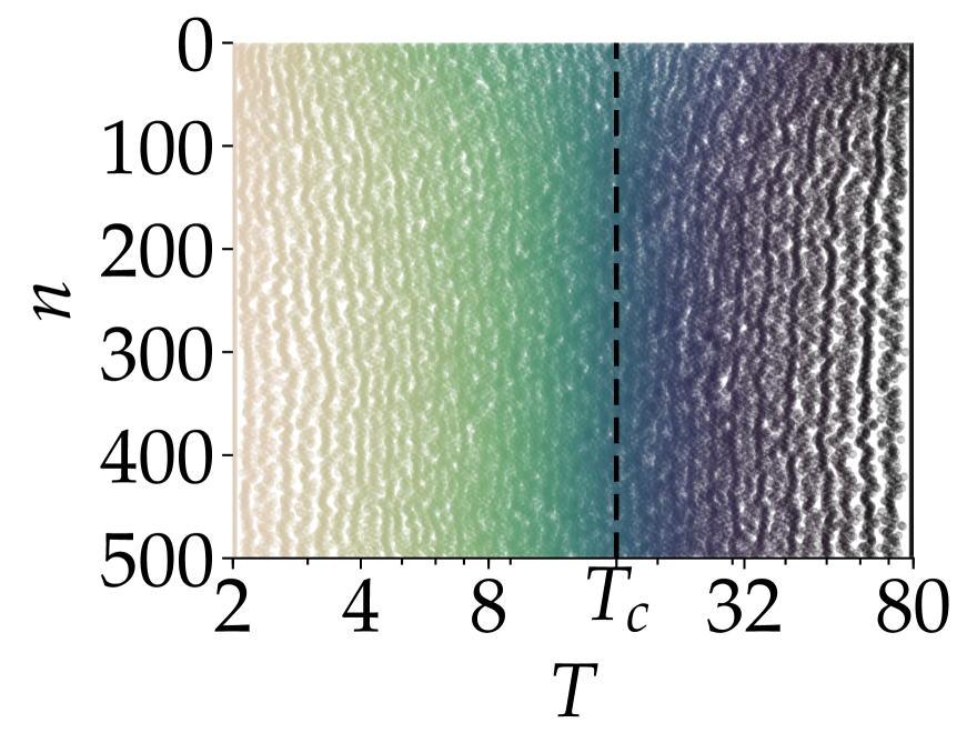
(a)           (a)

(b)           (b)

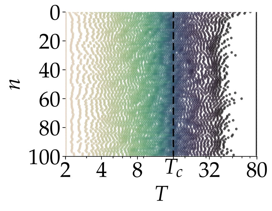
(c)           (c)

(d)           (d)

Figure 2: Evolution of the temperature set through $500$ iterations of the energy method, starting from a geometric distribution in (a), and from a uniform distribution in (b); the evolution of the temperature set over $100$ iterations of the feedback-optimized method, starting from a geometric distribution in (c), and from a uniform distribution in (d). All experiments have been performed on an SK-bimodal problem instance of size $256$. The vertical dashed lines indicate the value of the critical temperature $T_{c}$ that roughly equals $\sqrt{N}$ for a fully connected spin-glass problem with bimodal disorder.

As illustrated in Fig. 2, it takes around $200$ iterations, each with $200$ sweeps, for the energy method to converge to a stable replica distribution when initialized from a geometric distribution, and even more iterations when starting from a uniform distribution. The feedback-optimized method, independent of the initial condition, converges after around five iterations, however, and each iteration performs $20\,000$ sweeps. It is worth noting that our experiments have shown that the feedback-optimized method is more prone to divergence. That is, after a number of iterations, the flow can become disconnected if one of the replicas fails to reach either the highest or the lowest temperature. The energy method, in contrast, reliably converges given a sufficient number of iterations.

IV.3 Performance comparison

To quantify how the PT algorithm scales as the problem size increases using various replica distributions, we have measured the TTS. To observe the correct scaling of the PT algorithm, the minimum TTS for each problem class and size has been found by optimizing over the number of sweeps experimentally. More specifically, we have searched over different values of the number of sweeps, per problem class and size, to find the optimal number of sweeps that minimizes the TTS on a subset of problem instances. The TTS value, the acceptance probabilities of replica-exchange moves ($\mathcal{P}_{\mbox{\scriptsize{RE}}}$), and the MC acceptance probabilities ($\mathcal{P}_{\mbox{\scriptsize{MC}}}$) have been then measured for each problem class and size using all $100$ instances and the optimized number of sweeps.

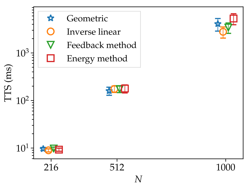
(a)          (a)

(b)          (b)

Figure 3: The median TTS as a function of the number of variables $N$ for (a) 3D-bimodal and (b) 4D-bimodal spin-glass problems.

Sparse Spin-Glass Problems

Figure 3 shows the mean and the standard deviation of the median TTS distribution of PT using four different temperature setting methods on 3D and 4D problems. In all subsequent TTS plots, points and error bars represent the mean and the standard deviation of the distribution of the median TTS. On both of these problem classes, the dynamic temperature setting methods do not outperform the static distributions for any of the three problem sizes. In terms of the fraction of problems solved to the best-known energy, all methods have solved more than $95\%$ of the problems in each class for the first two sizes. For the largest size, the inverse-linear distribution has solved the most: 91% and 98% for 3D and 4D, respectively. Conversely, the energy method has solved the fewest problems to the best-known energy: 78% and 89% for 3D and 4D, respectively.

Figures 4 and 5 illustrate the temperature distribution and the acceptance probabilities including the replica-exchange probability ($\mathcal{P}_{\mbox{\scriptsize{RE}}}$) at each replica, and the MC acceptance probability ($\mathcal{P}_{\mbox{\scriptsize{MC}}}$) at each replica for an instance of the largest problem size in each problem category of 3D-bimodal and 4D-bimodal.

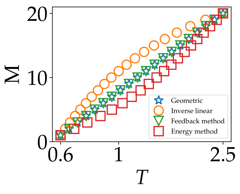
(a)         (a)

(b)         (b)

Figure 4: The cumulative number of temperatures below temperature $T$ (in log scale) obtained using four temperature setting methods for (a) a 3D-bimodal instance with $1000$ variables and for (b) a 4D-bimodal instance with $1296$ variables.

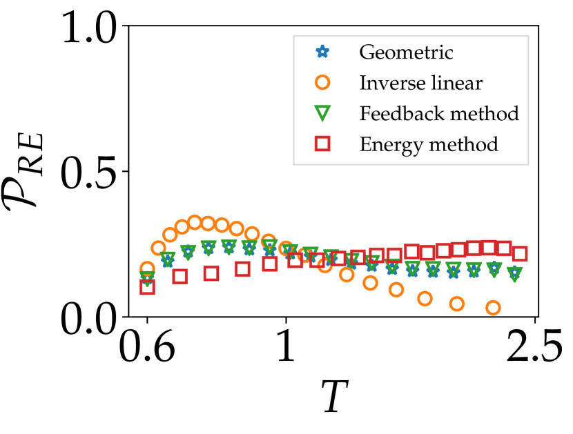
(a)        (a)

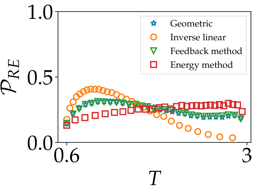
(b)        (b)

(c)        (c)

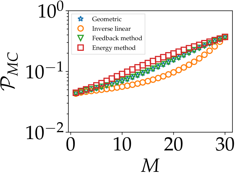
(d)        (d)

Figure 5: The acceptance probabilities of replica-exchange moves ($\mathcal{P}_{\mbox{\scriptsize{RE}}}$), and the MC acceptance probabilities ($\mathcal{P}_{\mbox{\scriptsize{MC}}}$) obtained using four methods for a 3D-bimodal instance with $1000$ variables are shown in (a) and (c), respectively. The same measurements are illustrated, in respective terms, for a 4D-bimodal instance with $1296$ variables in (b) and (d). The standard deviations for the MC probabilities are very small, and so have not been included. Those for replica-exchange probabilities were also excluded, but in this case for better readability.

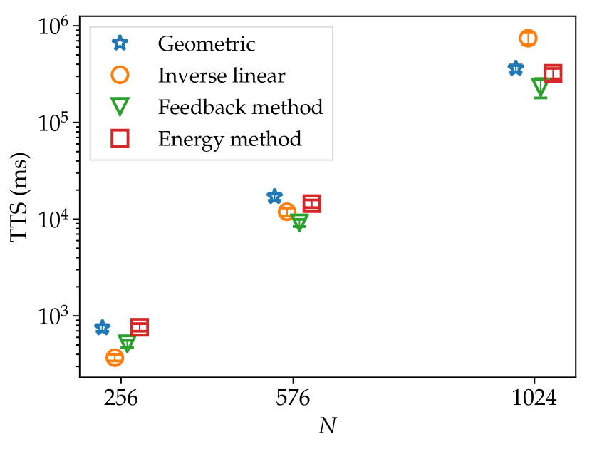
(a)          (a)

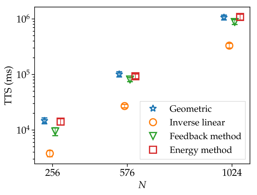
(b)          (b)

Figure 6: The median TTS of fully connected SK spin-glass problems with (a) bimodal and (b) Gaussian disorder versus the number of variables $N$.

Figure 4 illustrates that the feedback-optimized method does not improve on its initial temperature schedule, that is, the geometric distribution. In other words, the geometric distribution on sparse spin-glass problems turns out to have a closer flow to the optimal flow. Consequently, as shown in Fig. 5, both feedback-optimized and geometric temperature schedules demonstrate similar $\mathcal{P}_{\mbox{\scriptsize{RE}}}$ and $\mathcal{P}_{\mbox{\scriptsize{MC}}}$ distributions. The energy method, in contrast, changes its initial distribution: It has arranged fewer temperature values around the minimum temperature value, which results in a more uniform $\mathcal{P}_{\mbox{\scriptsize{RE}}}$ distribution, and has higher $\mathcal{P}_{\mbox{\scriptsize{MC}}}$ values. Having fewer temperatures close to the lowest temperature could indicate that the diffusion process that distributes replicas could require a much longer time to converge to the schedule with uniform swap rate. This may explain the slightly worse performance of the energy method for the largest problem size compared to the other three methods. The small performance improvement of the inverse-linear temperature method is likely due to the fact that its temperature distribution has the highest density around the minimum temperature value, its $\mathcal{P}_{\mbox{\scriptsize{RE}}}$ distribution has a large peak at low temperature values, and its $\mathcal{P}_{\mbox{\scriptsize{MC}}}$ values are the lowest.

Fully connected spin-glass problems

Figure 6 illustrates the mean and the standard deviation of the median TTS of PT using four temperature setting methods on the SK-bimodal and SK-Gaussian problem classes. Similarly to the sparse spin-glass problems, none of the dynamic temperature setting methods shows a clear advantage over the static replica distribution methods. The inverse-linear temperature set, however, has noticeably superior performance compared to the other methods for the SK-Gaussian problem class.

As shown in Fig. 7, for both the SK-bimodal and SK-Gaussian problem classes, the inverse-linear temperature schedule has arranged more temperature values close to the minimum temperature, resulting in similar $\mathcal{P}_{\mbox{\scriptsize{RE}}}$ and $\mathcal{P}_{\mbox{\scriptsize{MC}}}$ distributions. However, for the former class, the inverse-linear schedule yields poor performance, whereas for the latter, it results in a performance advantage. This behavioural difference is likely due to the fact that the replica-exchange probabilities for SK-bimodal problem instances are very close to zero for the replicas associated with temperature values between $20$ and $80$ (Fig. 8). Having near-zero exchange probabilities at high temperature values does not allow for a continuous reseeding of the states in the PT algorithm. In contrast, the replica-exchange probability values for SK-Gaussian problem instances are much higher over the same temperature range.

\begin{overpic}[width=433.62pt]{SK_Bimodal_temps.pdf} \end{overpic}

(a) (a)

\begin{overpic}[width=433.62pt]{SK_Gaussian_temps.pdf} \end{overpic}

(b) (b)

Figure 7: The cumulative distribution of number of temperatures obtained for a fully connected SK spin-glass problem instance with $1024$ variables with (a) bimodal and (b) Gaussian couplings using different temperature setting methods. The temperature values shown on the $x$-axis are in log scale.

(a)        (a)

(b)        (b)

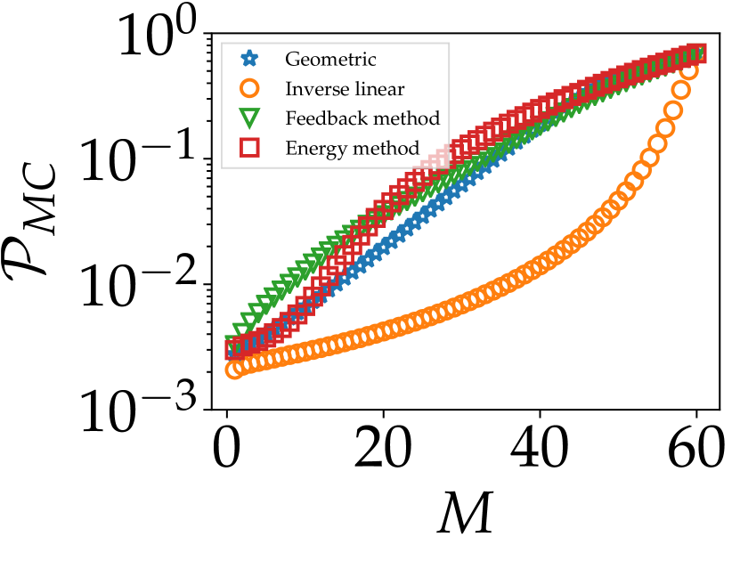
(c)        (c)

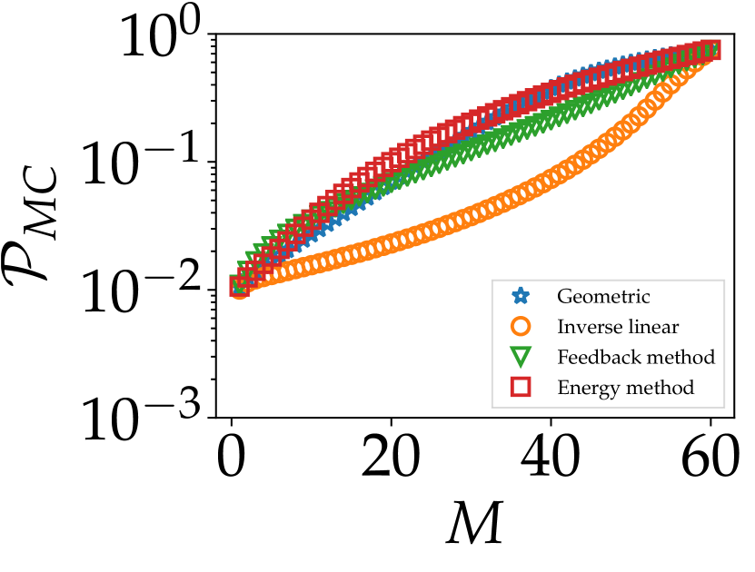
(d)        (d)

Figure 8: Replica-exchange ($\mathcal{P}_{\mbox{\scriptsize{RE}}}$) and MC ($\mathcal{P}_{\mbox{\scriptsize{MC}}}$) acceptance probability distributions of an instance of the SK-bimodal problem class with $1024$ variables are shown in (a) and (c), respectively, for different temperature setting methods. The same measurements are illustrated, in respective terms, for an SK-Gaussian problem instance with $1024$ variables in (b) and (d).

Our results for sparse and fully connected spin-glass problems that have continuous phase transitions in the order parameter do not show an advantage for the feedback-optimized method. The base inverse-linear method that places more temperature values around the minimum temperature results in better performance at a much lower computational cost.

Fully connected Wishart problems

The mean and the standard deviation of the median TTS for the PT algorithm for two relatively small-sized Wishart problems are shown in Fig. 9. The dynamic feedback-optimized temperature setting method exhibits a TTS that is approximately two times faster than the inverse-linear method and roughly five times faster than the energy and the geometric methods. Due to the inherent computational difficulty built into Wishart problems, we have been unable to solve a sufficient number of larger Wishart problem instances to optimality in order to measure the median TTS for bigger problem sizes.

\begin{overpic}[width=433.62pt]{SK_Wishart_tts_scaling.pdf} \end{overpic}

Figure 9: The median TTS of fully connected Wishart problems versus the number of variables $N$.

A closer look into the results shown in Fig. 10 and Fig. 11 demonstrates that, for Wishart problems, the energy method essentially converges to its initial geometric schedule, whereas the feedback method and the inverse-linear methods place twice as many replicas at or below the critical temperature. As mentioned in Sec. II.2, the energy method is designed to have equal replica-exchange probabilities for all adjacent temperature values. Despite the roughly uniform $\mathcal{P}_{\mbox{\scriptsize{RE}}}$ distribution of the energy method for the previous two problem classes, the energy method results in a nonuniform distribution for Wishart problem instances.

In contrast to spin-glass problems, the Wishart problems have a first-order phase transition. As shown in Fig. 11, the feedback-optimized method distributes the temperature values such that the replica-exchange probabilities are the highest around the critical temperature ($T_{c}\simeq 0.25$), compared to the other temperature setting methods. This maximizes the temperature mixing around the critical temperature and consequently yields a smaller value for the TTS.

\begin{overpic}[width=433.62pt]{SK_Wishart_temps.pdf} \end{overpic}

Figure 10: The cumulative distribution of number of temperatures obtained for a fully connected Wishart problem instance of size $128$ using four temperature setting methods. The temperature values shown on the $x$ axis are in log scale.

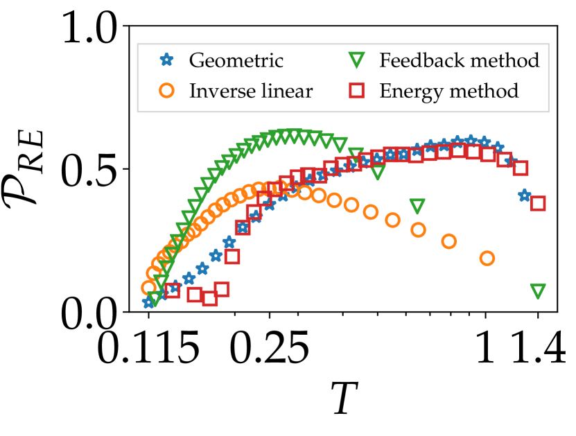
(a)        (a)

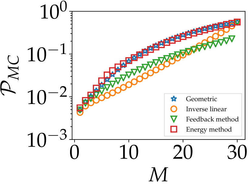
(b)        (b)

Figure 11: Acceptance probabilities for replica-exchange moves ($\mathcal{P}_{\mbox{\scriptsize{RE}}}$) and MC acceptance probabilities ($\mathcal{P}_{\mbox{\scriptsize{MC}}}$) obtained using four methods for a Wishart instance of size $128$ are shown in (a) and (b), respectively.

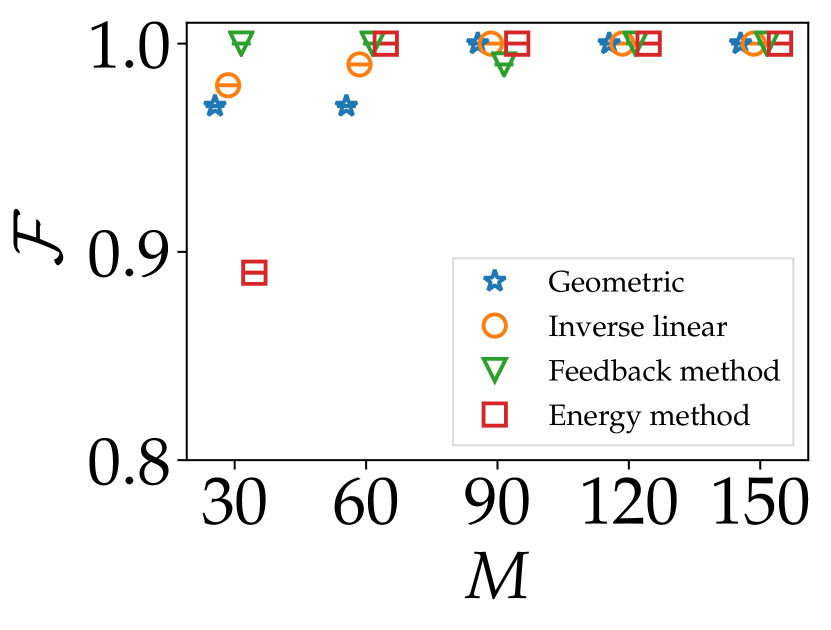
(a)        (a)

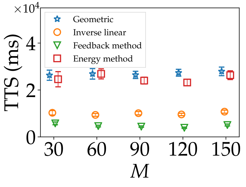
(b)        (b)

Figure 12: (a) Fraction of problems solved, $\mathcal{F}$, and (b) median TTS versus the number of replicas, $M$, for various temperature setting methods and for Wishart problems with $N=128$.

To investigate how the performance of the feedback-optimized method is affected as the number of replicas increases, the fraction of problems solved to optimality, $\mathcal{F}$, and the median TTS values are shown in Fig. 12 for various numbers of replicas for a problem with $128$ variables. The feedback-optimized method solves all problem instances to optimality starting from $30$ replicas, whereas the other methods require at least $90$ replicas to solve all problem instances to optimality. The difference between the TTS of the feedback-optimized method and the other methods remains relatively constant for varying numbers of replicas.

V Conclusion

In this paper, we have compared the performance of four temperature setting techniques, the feedback-optimized method, the energy method, and two base methods (geometric and inverse-linear), all using random instances of spin-glass and Wishart problems.

The feedback-optimized and the energy methods are dynamic approaches that rely on measuring statistical properties, such as local diffusivity and average energy, in respective terms, to iteratively adjust temperature values. The former method aims for a nonuniform replica-exchange probability by increasing the density of the temperature values around the simulation bottlenecks. The latter method, however, is designed to ensure constant probability across neighboring replicas.

Our results support the superiority of the feedback-optimized method on Wishart problems that have first-order phase transitions at low temperatures. The replica-exchange probability has its highest density at the vicinity of the critical temperature ($T_{c}\simeq 0.25$). More specifically, the feedback-optimized method results in a TTS speedup of a factor of two and five, compared to the inverse-linear method and to the energy and the geometric methods, respectively. On spin-glass problems with a continuous transition between the disordered and ordered phases at critical temperatures, the computational overhead of the two dynamic temperature setting methods, feedback-optimized and energy, does not yield any performance advantage over the base methods. In this case, the inverse-linear method that arranges more temperature values close to the lowest temperature outperforms the other methods.

In summary, our work provides experimental evidence that the optimization problems, especially those with discontinuous transitions, are well suited to benefit from nonuniform and temperature-dependent acceptance probabilities for swap moves when using the PT algorithm.

References

- Geyer (1991) C. Geyer, in 23rd Symposium on the Interface, edited by E. M. Keramidas (Interface Foundation, Fairfax Station, VA, 1991), p. 156.
- Swendsen and Wang (1986) R. H. Swendsen and J.-S. Wang, Replica Monte Carlo simulation of spin-glasses, Phys. Rev. Lett. 57, 2607 (1986).
- Hukushima and Nemoto (1996) K. Hukushima and K. Nemoto, Exchange Monte Carlo method and application to spin glass simulations, J. Phys. Soc. Jpn. 65, 1604 (1996).
- Earl and Deem (2005) D. J. Earl and M. W. Deem, Parallel tempering: Theory, applications, and new perspectives, Phys. Chem. Chem. Phys. 7, 3910 (2005).
- Katzgraber (2009) H. G. Katzgraber, Introduction to Monte Carlo methods (2009), (arXiv:0905.1629).
- Moreno et al. (2003) J. Moreno, H. G. Katzgraber, and A. K. Hartmann, Finding low-temperature states with parallel tempering, simulated annealing and simple monte carlo, International Journal of Modern Physics C 14, 285 (2003).
- Mandrà et al. (2016) S. Mandrà, Z. Zhu, W. Wang, A. Perdomo-Ortiz, and H. G. Katzgraber, Strengths and weaknesses of weak-strong cluster problems: A detailed overview of state-of-the-art classical heuristics versus quantum approaches, Physical Review A 94, 022337 (2016).
- Zhu et al. (2016) Z. Zhu, C. Fang, and H. G. Katzgraber, borealis - A generalized global update algorithm for Boolean optimization problems (2016), (arXiv:1605.09399).
- Rathore et al. (2005) N. Rathore, M. Chopra, and J. J. de Pablo, Optimal allocation of replicas in parallel tempering simulations, J. Chem. Phys. 122, 024111 (2005).
- Hamze et al. (2010) F. Hamze, N. Dickson, and K. Karimi, Robust parameter selection for parallel tempering, Int J Mod Phys C 21, 603 (2010).
- Kofke (2004) D. A. Kofke, Comment on ”The incomplete beta function law for parallel tempering sampling of classical canonical systems” [J. Chem. Phys. 120, 4119 (2004)], J. Chem. Phys. 121, 1167 (2004).
- Predescu et al. (2005) C. Predescu, M. Predescu, and C. Ciobanu, On the efficiency of exchange in parallel tempering Monte Carlo simulations, J. Phys. Chem. B 109, 4189 (2005).
- Fiore (2008) C. E. Fiore, First-order phase transitions: A study through the parallel tempering method, Phys. Rev. E 78, 041109 (2008).
- Machta (2009) J. Machta, Strengths and weaknesses of parallel tempering, Phys. Rev. E 80, 056706 (2009).
- Machta and Ellis (2011) J. Machta and R. Ellis, Monte Carlo methods for rough free energy landscapes: Population annealing and parallel tempering, J. Stat. Phys. 144, 541 (2011).
- Predescu et al. (2004) C. Predescu, M. Predescu, and C. V. Ciobanu, The incomplete beta function law for parallel tempering sampling of classical canonical systems, J. Chem. Phys 120 9, 4119 (2004).
- Hukushima (1999) K. Hukushima, Domain-wall free energy of spin-glass models: Numerical method and boundary conditions, Phys. Rev. E 60 (1999).
- Trebst et al. (2004) S. Trebst, D. A. Huse, and M. Troyer, Optimizing the ensemble for equilibration in broad-histogram Monte Carlo simulations, Phys. Rev. E 70 (2004).
- Katzgraber et al. (2006) H. G. Katzgraber, S. Trebst, D. A. Huse, and M. Troyer, Feedback-optimized parallel tempering Monte Carlo, J. Stat. Mech. P03018 (2006).
- Hamze et al. (2019) F. Hamze, J. Raymond, C. A. Pattison, and H. G. Katzgraber, The Wishart planted ensemble: A tunably-rugged pairwise Ising model with a first-order phase transition (2019), https://arxiv.org/abs/1906.00275.
- Wang et al. (2015) W. Wang, J. Machta, and H. G. Katzgraber, Comparing Monte Carlo methods for finding ground states of Ising spin glasses: Population annealing, simulated annealing, and parallel tempering, Phys. Rev. E 92, 013303 (2015).
- Atkins and De Paula (2006) P. Atkins and J. De Paula, Physical Chemistry for the Life Sciences (Oxford University Press, 2006).
- Steffen (1990) M. Steffen, A simple method for monotonic interpolation in one dimension, Astron. Astrophys. 239 (1990).
- Pardella and Liers (2008) G. Pardella and F. Liers, Exact ground states of large two-dimensional planar Ising spin glasses, Phys. Rev. E 78, 056705 (2008).
- Liers and Pardella (2010) F. Liers and G. Pardella, Partitioning planar graphs: A fast combinatorial approach for max-cut, Comput. Optim. Appl. p. 1 (2010).
- Elf et al. (2001) M. Elf, C. Gutwenger, M. Jünger, and G. Rinaldi, Lecture notes in computer science 2241, in Computational Combinatorial Optimization, edited by M. Jünger and D. Naddef (Springer Verlag, Heidelberg, 2001), vol. 2241.
- Grötschel et al. (1987) M. Grötschel, M. Jünger, and G. Reinelt, in Heidelberg colloquium on glassy dynamics (Springer, 1987), p. 325.
- Sherrington and Kirkpatrick (1975) D. Sherrington and S. Kirkpatrick, Solvable model of a spin glass, Phys. Rev. Lett. 35, 1792 (1975).
- Rønnow et al. (2014) T. F. Rønnow, Z. Wang, J. Job, S. Boixo, S. V. Isakov, D. Wecker, J. M. Martinis, D. A. Lidar, and M. Troyer, Defining and detecting quantum speedup, Science 345, 420 (2014).
- Aramon et al. (2019) M. Aramon, G. Rosenberg, E. Valiante, T. Miyazawa, H. Tamura, and H. G. Katzgraber, Physics-inspired optimization for quadratic unconstrained problems using a digital annealer, Frontiers in Physics 7, 48 (2019).
- (31) http://informatik.uni-koeln.de/spinglass.