Residual Entropy

Abstract

We describe an approach to improving model fitting and model generalization that considers the entropy of distributions of modelling residuals. We use simple simulations to demonstrate the observational signatures of overfitting on ordered sequences of modelling residuals, via the autocorrelation and power spectral density. These results motivate the conclusion that, as commonly applied, the least squares method assumes too much when it assumes that residuals are uncorrelated for all possible models or values of the model parameters. We relax these too-stringent assumptions in favour of imposing an entropy prior on the (unknown, model-dependent, but potentially marginalizable) distribution function for residuals. We recommend a simple extension to the Mean Squared Error loss function that approximately incorporates this prior and can be used immediately for modelling applications where meaningfully-ordered sequences of observations or training data can be defined.

1 Introduction

The method of least squares is the dominant approach in regression problems. The Mean Squared Error (MSE) is frequently therefore the default loss function in many practical applications: and is commonly used for regression in fields as diverse as machine learning, statistics, physical sciences, decision theory, econometrics, and finance. It is criticised for over-use and a lack of robustness [e.g. 2], but has yet to be displaced. In this paper we will level another criticism at the MSE and other similarly-constructed loss functions: they leave out important information as a result of their too-strict assumptions about the uncorrelatedness of model residuals.

Statistical analysis of correlated residuals has a long history in econometrics and time series analysis, that began with tests of the presence of autocorrelation at lag $l=1$ in residuals from least squares regression [17, 6, 7, 8]. Tests were later developed for the presence of autocorrelation at any lag [3, 13]. The question became acute as econometrics developed, as autocorrelations in residuals for autoregressive time series models (where some of the regressors are lagged dependent variables) leads in general to non-consistency and bias. Sophisticated tests have therefore been developed to help validate such models [4, 9, 15] and make them robust to further confounding real-world factors such as conditional heteroskedasticity [e.g. 10].

While prior work in this area has to been to devise tests of autocorrelation that can be applied after best-fitting regression models have been determined, e.g. by least squares, we propose that the loss function itself could be extended to penalize models showing autocorrelated residuals during the process of fitting. Such correlations can either be created by the presence of correlated errors in observations of the independent variable, or by the application of the wrong model. In the first Section we illustrate this for the important category of overfitting (or over-specified) models by performing simple simulations of model fitting in one dimension.

In later Sections we make a simple entropy argument for an extension to the MSE loss function that is readily and efficiently calculated, at least in one dimension or wherever residuals can be meaningfully ordered (e.g. time series forecasting). We illustrate from our simulations how this modified loss function will effectively penalize overfitting models, potentially providing natural regularization, better generalization and enhanced robustness to outliers.

2 Simulations of Overfitting in One Dimension

Consider a sample $Y=\left(y_{0},y_{1},\ldots,y_{N-1}\right)$ of $N$ data values for our dependent variable of interest $y$, situated at corresponding locations $\left(x_{0},\ldots,x_{N-1}\right)$ in the indpendent variable. We will construct a regression model for estimates of $y$ which we will denote $\hat{y}(x|\bm{\theta})$ for a vector of model parameters $\bm{\theta}$. The residuals $R$ between the model and the data are defined as $R=(r_{0},\ldots,r_{N-1})$ where $r_{n}=y_{n}-\hat{y}(x_{n})$ for each element $n=0,\ldots,{N-1}$ of the sample.

To explore the effects of overfitting, we will draw $Y$ as i.i.d. standard normal variables, the distribution of residuals you would expect from a good fit to the data, and then attempt to fit these values. The aim is to simulate what happens when a model is given unnecessary additional freedom.

2.1 A Fourier Series Model

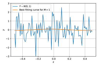
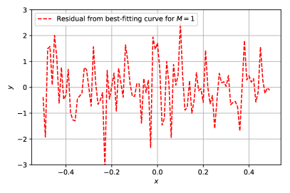
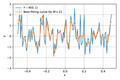
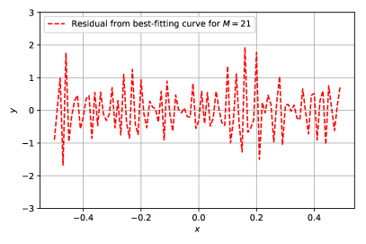
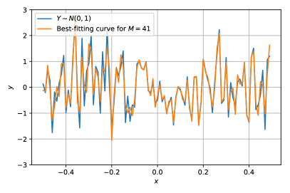
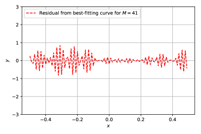
Figure 1: Three examples of randomly-drawn samples $Y$ and the least-squares best-fitting model (left column), and resulting residuals (right column), for model orders $M=1$ (top row), $M=21$ (middle row), and $M=41$ (bottom row) of the Fourier series model of equation (1). The residuals reduce in amplitude but also appear “less random” as the model order increases.

We simulate a simple case of $N=100$ observations for our randomly-drawn sample $Y$, with corresponding evenly-spaced locations $x_{n}=-0.5+n/N$ for $n=0,\ldots,{N-1}$. We define the model of order $M$ as a truncated Fourier Series:

$$\hat{y}_{\mathrm{s},M}\left(x|a_{0},a_{1},\ldots,a_{M-1},b_{1},\ldots,b_{M-1}\right)=\frac{1}{2}a_{0}+\sum_{m=1}^{M-1}a_{m}\cos{(2\pi mx)}+b_{m}\sin{(2\pi mx)}.$$ (1)

Figure 1 shows three examples of least-squares fitting $\hat{y}_{\mathrm{s},M}(x)$ to different randomly-generated samples $Y$, and the resulting residuals. We can see that as the overfitting order $M$ increases to 41 there is observable structure in the sequence of residuals $R$.

The aim of this paper is to show that there is valuable information about modelling in the way that residual values are distributed with respect to one another in the domain of input variables. The tools of correlation and spectral analysis are the primary aids for assessing these properties. We define the (circular) residual autocorrelation function at lag $l$ as

$$\rho_{rr}(l)\triangleq\left.\sum_{n=0}^{N-1}r_{n}(r_{N})^{*}_{n-l}\middle/\>\left(\sum_{n=0}^{N-1}r_{n}r^{*}_{n}\right)\right.,$$ (2)

where $r^{*}_{n}$ denotes the complex conjugate of $r_{n}$ (we will assume real-valued $r_{n}$ hereafter so that $r_{n}r^{*}_{n}=r^{2}_{n}$), and where $r_{N}$ denotes an element of the sequence $R$ extended by periodic summation to an infinitely long, repeating sequence of period $N$ so that for $p\in\mathbb{Z}$, we have $(r_{N})_{p}=r_{(p\!\!\!\mod\!N)}$.

The term in the denominator of (2), commonly referred to as the Residual Sum of Squares (RSS) or Sum of Squared Errors of prediction (SSE), normalizes the function so that $\rho_{rr}(l=0)\triangleq 1$. At lags $l\neq 0$ statistically independent residuals have $E(\rho_{rr})=0$. For purely real residuals (2) is an even symmetric function of $|l|$, and is Hermitian in general.

This definition of the residual autocorrelation function is convenient because it can be related simply to the Discrete Fourier Transform (DFT) of the sequence of residuals $\tilde{R}=\left(\tilde{r}_{0},\ldots,\tilde{r}_{k},\ldots,\tilde{r}_{N-1}\right)$, where

$$\tilde{r}_{k}=\sum_{n=0}^{N-1}r_{n}\,e^{-\frac{i2\pi}{N}kn}$$ (3)

and the inverse transform is defined as

$$r_{n}=\frac{1}{N}\sum_{k=0}^{N-1}\tilde{r}_{k}\,e^{\frac{i2\pi}{N}kn}.$$ (4)

We will often shorthand the DFT operations on a full sequence using the symbol $\mathcal{F}$, e.g. $\tilde{R}=\mathcal{F}\{R\}$ and $R=\mathcal{F}^{-1}\{\tilde{R}\}$. Using the circular form of the Wiener-Khinchin theorem for DFTs we may then write $\rho_{rr}(l)=\mathcal{F}^{-1}\{\tilde{R}\,\tilde{R}^{*}\}/\left(\sum_{n=0}^{N-1}r^{2}_{n}\right)$, which can be calculated with great computational efficiency thanks to the Fast Fourier Transform (FFT) algorithm [5].

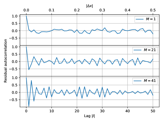
Figure 2: Residual autocorrelation function values for the randomly-drawn samples and least-squares best-fitting models of Figure 1.

Figure 2 shows $\rho_{rr}(l)$ for the model fits of Figure 1. Significant negative correlation between neighbouring residuals is seen at lag $|l|=1$ for the $M=21$ and $M=41$ models. The $M=41$ model shows the strongest departures from $\rho_{rr}\simeq 0$ at lags $l\neq 0$, with an oscillating character. Figure 3a, shows the average of residual autocorrelation values across $10^{5}$ independent realizations of $Y$ from a suite of simulations at each model order $M<50$. There is structure.

As well as being useful for the efficient calculation of $\rho_{rr}(l)$, the sequence $(\tilde{R}\,\tilde{R}^{*})$ is a powerful equivalent representation. It defines the power spectral density of our sequence of residuals, which we denote

$$P_{rr}(k)=(\tilde{R}\,\tilde{R}^{*})_{k}.$$ (5)

For later convenience we will also define a corresponding correlation spectral power density $\tilde{\rho}_{rr}(k)\triangleq P_{rr}(k)/\left(\sum_{n=0}^{N-1}r^{2}_{n}\right)$, the DFT of $\rho_{rr}(l)$. $P_{rr}(k)$ and $\tilde{\rho}_{rr}(k)$ are both even symmetric functions of $|k|$ for purely real residuals. For i.i.d. residuals with a defined variance, these functions are expected to show a flat, white noise spectrum with constant expectation values $E(P_{rr})=\sum_{n=0}^{N-1}r^{2}_{n},E(\tilde{\rho}_{rr})=1$ for all $k=0,\ldots,N-1$.

Figure 3b shows the averaged power spectral signature of residuals from the same suite of simulations as shown in Figure 3a, where we have defined the power spectral signature as

$$S_{rr}(k)=P_{rr}(k)/\max_{k}{\left\{P_{rr}\right\}},$$ (6)

for some sequence of residuals $R$ with power spectral density $P_{rr}(k)$. This choice makes the structure of the power spectrum easy to visualize: with increasing $M$, we see that an increasing share of the lower-$k$ spectral modes are suppressed, starting with the lowest $k$. The apparent structure in the modelling residuals from overfitting arises because these residuals no longer match the flat power spectrum distribution that would be expected if they could be assumed to be i.i.d. – in a very real sense they have been high-pass filtered.

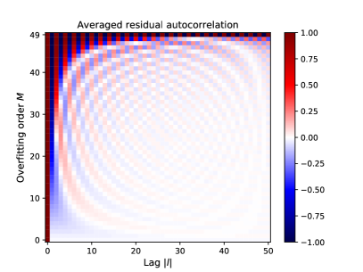
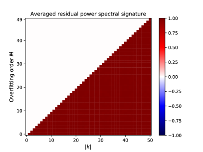
Figure 3: a) Averaged residual autocorrelation function values as a function of Fourier Series model order $M$, calculated over $10^{5}$ realizations of $Y$ per order; b) Averaged residual power spectral signature for the same realizations and model.

2.2 A Chebyshev Polynomial Series Model

The Fourier Series model (1) is a special case: it forms an othonormal basis, its coefficients $a_{m}$ and $b_{m}$ have direct correspondence to the real and imaginary parts of the DFT itself, and it provides an optimally compact (in terms of $M$) series representation of arbitrary real-valued sequences $R$.

The suppression of lower-$k$ power in $P_{rr}(k)$ by overfitting models in the simulations performed above is therefore, in fact, effectively total; not only on average but also in individual cases. In general models will often not have complete freedom to precisely replicate arbitrary variation in observed data (although see [18]), nor will they so wholly suppress Fourier modes in residuals.

For this reason it is interesting to generalize to a set of model basis functions that do not match the modes of the DFT precisely, and cannot represent arbitrary patterns of residuals in any finite series. Candidates for such a basis are the Chebyshev polynomials of the first kind, $T_{m}(x)$ (see [1]). We define the Chebyshev polynomial series model of order $M$ as:

$$f_{\mathrm{c},M}\left(x|a_{0},a_{1},\ldots,a_{M-1}\right)=\sum_{m=0}^{M-1}a_{m}T_{m}(x).$$ (7)

The absolute values of these functions are bounded by 1 on the interval $[-1,1]$, and they are a convenient basis for polynomial interpolation in bounded spaces. As for the Fourier Series, we simulate a simple case of $N=100$ observations in our sample $Y$. We place these at corresponding evenly-spaced locations $x_{n}=-1+2n/N$ for $n=0,\ldots,{N-1}$.

Once more, we performed $10^{5}$ independent realizations of $Y$ for each Chebyshev model order $M\leq 100$ (as the Chebyshev polynomial series model does not afford a complete representation of an arbitrary sequence $R$ at any level of truncation, unlike the Fourier Series, the choice of maxmimum $M$ is somewhat arbritrary). Figure 4 shows the averaged residual autocorrelation $\rho_{rr}(l)$ and power spectral signature $S_{rr}(k)$, as a function of order $M$, across this suite of simulations. We see similar behaviour to the Fourier Series case, with increasing modelling order $M$ leading to increasing supression of lower-$k$ power. Due to the less compact representation of arbitrary sequences provided by Chebyshev polynomials, the suppression of lower-$k$ power by overfitting is more gradual.

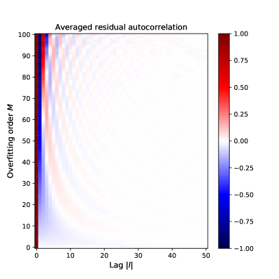
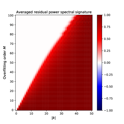
Figure 4: a) Averaged residual autocorrelation function values as a function of Chebyshev polynomial model order $M$, calculated over $10^{5}$ realizations of $Y$ per order; b) Averaged residual power spectral signature for the same realizations and model.

3 Implications for the Mean Squared Error Loss Function

As discussed in Section 1, the MSE loss function is very commonly used in optimization and regression applications, and is defined using the notation above as simply $\textrm{MSE}(R)=\frac{1}{N}\sum_{n=0}^{N-1}r^{2}_{n}$. Underpinning the widespread use of the MSE as a loss function is the Gauss-Markov theorem: that for a linear model fit to observations with uncorrelated, equal variance and zero mean errors, the best linear unbiased estimator of any linear combination of the observations is that which minimizes the MSE. Where observational errors can be assumed to also follow a Gaussian distribution, this estimator is also the Maximum Likelihood Estimator (e.g. [14]).

But we have seen that residuals are not necessarily uncorrelated. The model residuals passed to the MSE loss function will only be uncorrelated in general if the ‘true’ model has been applied, and the model parameters $\bm{\theta}$ are optimal. Anything else will, in general, either underfit or overfit, introducing correlations as shown above and as discussed (in a specific application) by [16]. In empirical settings and machine learning applications the ‘true’ model may be unknown and potentially unknowable. The application of the MSE loss function in regression tasks, often by default, assumes too much in assuming that model residuals are uncorrelated – irrespective of model selection or under variation in model parameter values – however plausible this assumption may be about the underlying observational errors. This causes us to unwittingly discard valuable information.

The information discarded is not captured by the MSE, which is invariant under permutation of any ordered sequence of the residual, because it is embedded within knowledge of the relative locations of residuals with respect to one another. The aim of this paper is to make initial step towards using this information in the optimization process so as to build better regularized, and better generalizing, models. If this can be done at all, computational efficiency and ease of adoption will be valuable characteristics of the solution. With these aims in mind, we will explicitly target as simple a modification of the widely-used MSE loss function as possible.

4 Incorporating Knowledge of Correlated Residuals into the Loss Function

4.1 A Multivariate Gaussian Distribution & The Least Squares Case

We begin with the simplest possible applicable probabily distribution for correlated residuals, a multivariate Gaussian. We write the probability density function as

$$p(r_{0},\dots,r_{N-1})=\frac{1}{\sqrt{(2\pi)^{N}\det{(\mathbf{\Sigma})}}}\exp{\left[-\frac{1}{2}\left(\mathbf{r}-\bm{\mu}\right)^{\mathrm{T}}\mathbf{\Sigma}^{-1}\left(\mathbf{r}-\bm{\mu}\right)\right]}$$ (8)

where for convenience we have adopted vector notation to describe the sequence of residuals $\mathbf{r}=(r_{0},\ldots,r_{N-1})^{\mathrm{T}}$, with corresponding mean $\bm{\mu}$ and covariance matrix $\mathbf{\Sigma}$. We will assume $\bm{\mu}=0$.

For ordinary least squares it would be additionally assumed that $\mathbf{\Sigma}=\sigma^{2}\mathbf{I}_{N}$, where $\mathbf{I}_{N}$ is the $N\times N$ identity matrix. and $\sigma^{2}$ is the variance of errors. Then identifying (8) with the statistical likelihood of the model $\mathcal{L}(\mathbf{y},\hat{\mathbf{y}}|\bm{\theta},\sigma^{2})$ leads to the log-likelihood function

$$\ln{\left[\mathcal{L}(\mathbf{y},\hat{\mathbf{y}}|\bm{\theta},\sigma^{2})\right]}=-\frac{N}{2\sigma^{2}}\textrm{MSE}(\mathbf{y},\hat{\mathbf{y}}|\bm{\theta})-\frac{N}{2}\ln{\left(2\pi\sigma^{2}\right)}.$$ (9)

Minimizing the MSE therefore maximizes the likelihood, irrespective of any value taken by the (likely unknown) variance $\sigma^{2}$.

4.2 A New Loss Function

We will seek a new loss function of the form $L(\mathbf{y},\hat{\mathbf{y}}|\bm{\theta})=\textrm{MSE}(\mathbf{y},\hat{\mathbf{y}}|\bm{\theta})+X(\mathbf{y},\hat{\mathbf{y}}|\bm{\theta})$, where the function $X$ is to be determined. To identify a candidate, we will relax assumptions about the covariance matrix of residuals in (8) relative to the least squares case, and instead assume the slightly more general

$$\mathbf{\Sigma}=\sigma^{2}\mathbf{P}$$ (10)

where $\mathbf{P}$ is an $N\times N$, symmetric, positive semidefinite correlation matrix with unit values on the diagonals. We will have little a priori knowledge of the contents of $\mathbf{P}$, which as we know from Section 2 can vary with model and model parameters, as well as with any correlations that may existing in the underlying observational errors.

We propose to weaken the common assumption that $\mathbf{P}=\mathbf{I}_{n}$ by instead introducing the following form for the prior probability on $\mathbf{P}$:

$$p(\mathbf{P})\propto\exp{\left[\eta\times h(\mathbf{P})\right]},$$ (11)

where $h(\mathbf{P})=\frac{N}{2}(1+\ln{2\pi})+\frac{1}{2}\ln{[\det(\mathbf{P})]}$ is the differential entropy for a multivariate Gaussian with covariance matrix $\mathbf{P}$, and $\eta$ is a scaling constant that we introduce to allow the user to balance the contribution to the loss function from this prior. The prior can then be simplified to

$$p(\mathbf{P})\propto\left[\det{(\mathbf{P})}\right]^{\frac{\eta}{2}}.$$ (12)

We motivate the functional form of (11) by direct analogy to the Boltzmann entropy formula (e.g. [11]), in the intuitive belief that the most likely distribution of residuals is that which has the greatest number of possible configurations per unit of variance. As $\det{(\mathbf{P})}$ is maximized when $\mathbf{P}=\mathbf{I}_{n}$, applying this prior will penalize distributions of residuals showing any correlations, whether from overfitting or underfitting [16].

Crucially, we will also assume that $\mathbf{P}$ can be approximated as a circulant matrix. (Although not true in general, particularly for small samples, the approximation becomes asymptotically more accurate as $N$ increases and/or as residual correlations themselves become negligible, since $\mathbf{I}_{N}$ is a circulant matrix.) Any circulant matrix $\mathbf{P}$ is fully determined by its first column which we label $\bm{\rho}$.

As $\mathbf{P}$ is a correlation matrix, the column $\bm{\rho}$ consists of the ‘true’ values around which the (circular) residual autocorrelation function $\rho_{rr}(l)$ of equation (2), defined for a single sample of residual values, will be distributed. It can be seen that the average of $\rho_{rr}(l)$ over realizations of residuals from multiple independent samples of observations $Y$, given the same model, will form an asymtotically consistent estimator for $\bm{\rho}$. But for any sufficiently free, circulant matrix model of $\mathbf{P}$ even a single sample of residuals allows us to calculate a $\rho_{rr}(l)$ that can itself be identified as the maximum likelihood estimate of $\bm{\rho}$; we will denote this estimate $\bar{\bm{\rho}}=\rho_{rr}(l)$. If $\mathbf{P}$ is assumed circulant this also defines a corresponding maximum likelihood estimate for the full matrix, $\bar{\mathbf{P}}(\mathbf{y},\hat{\mathbf{y}}|\bm{\theta})$.

If $\mathbf{P}$ is a circulant matrix its eigenvalues are the DFT of $\bm{\rho}$. The same holds for the eigenvalues of $\bar{\mathbf{P}}$:

$$(\lambda_{\bar{\mathbf{P}}})_{k}=\left[\mathcal{F}\left\{\bar{\bm{\rho}}\right\}\right]_{k}=\tilde{\rho}_{rr}(k),$$ (13)

where $k=0,\ldots,N-1$. Since the determinant of a matrix is given by the product of its eigenvalues, $\det{(\bar{\mathbf{P}})}$ can be written as

$$\det{\left[\bar{\mathbf{P}}(\mathbf{y},\hat{\mathbf{y}}|\bm{\theta})\right]}=\prod_{k=0}^{N-1}(\lambda_{\bar{\mathbf{P}}})_{k}=\prod_{k=0}^{N-1}\tilde{\rho}_{rr}(k).$$ (14)

As discussed above, the MSE loss function can be related to the log-likelihood function of the multivariate Gaussian with uncorrelated residuals. In a full, formally-correct treatment this likelihood should be expanded to include a freely-varying $\mathbf{P}$ which can then be marginalized over as a nuisance parameter, combining both the prior $p(\mathbf{P})$ and the likelihood of observed correlated residuals given $\mathbf{P}$ in the integrand. But this is reserved for future work. Instead we propose an approximate treatment that assumes that the likelihood of any observed residual correlations given some $\mathbf{P}$ can be approximated as very sharply peaked, indeed as being a Dirac delta function $\delta\left(\mathbf{P}-\bar{\mathbf{P}}\right)$, around $\bar{\mathbf{P}}$. This makes the marginalization trivial to compute, and adding a penalty term $-\ln{\left[p(\bar{\mathbf{P}})\right]}$ to the multivariate Gaussian log-likelihood of (9) to create new loss function:

$$L(\mathbf{y},\hat{\mathbf{y}}|\bm{\theta})=-\ln{\left[\mathcal{L}(\mathbf{y},\hat{\mathbf{y}}|\bm{\theta})\right]}-\ln{\left[p(\bar{\mathbf{P}}(\mathbf{y},\hat{\mathbf{y}}|\bm{\theta}))\right]}+\ldots,$$ (15)

where we will now omit terms that have no dependence on the parameter vector $\bm{\theta}$. Dividing both sides by $N/\sigma^{2}$ we arrive at the equivalent

$$L(\mathbf{y},\hat{\mathbf{y}}|\bm{\theta})=\textrm{MSE}(\mathbf{y},\hat{\mathbf{y}}|\bm{\theta})-\sigma^{2}\frac{\eta}{N}\sum_{k=0}^{N-1}\ln{\left[\tilde{\rho}_{rr}(k)\right]}.$$ (16)

Defining the Mean Log Power of residual correlations as $\textrm{MLP}=\frac{1}{N}\sum_{k=0}^{N-1}\ln{\left[\tilde{\rho}_{rr}(k)\right]}$, and making a final approximation that the MSE is a consistent, sufficient estimator for $\sigma^{2}$ (valid in the limit $\mathbf{P}\rightarrow\mathbf{I}_{n}$) we arrive at the following proposal for a residual entropy-sensitive extension of the MSE loss function:

$$L(\mathbf{y},\hat{\mathbf{y}}|\bm{\theta})=\textrm{MSE}(\mathbf{y},\hat{\mathbf{y}}|\bm{\theta})\times\left[1-\eta\>\textrm{MLP}(\mathbf{y},\hat{\mathbf{y}}|\bm{\theta})\right].$$ (17)

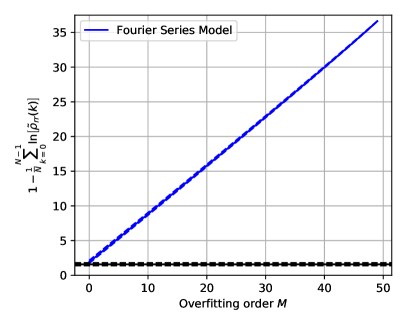
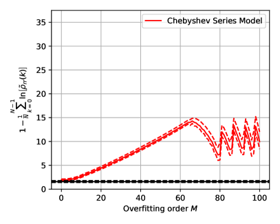
Figure 5: a) Median (solid blue line) and 5th, 95th percentile boundaries (dashed blue lines) of values of $\left[1-\textrm{MLP}(R)\right]$ for the simulations of Section 2.1, as a function of Fourier Series model order $M$: the black lines show the distribution of this quantity estimated from $Y$ in the absence of any model fit; b) The same but for the Chebyshev simulations of Section 2.2 (red lines): following investigation we have concluded that the structure seen at high $M$ values is due to low-level aliasing artifacts introduced by the significant variation in the higher-order Chebyshev polynomials at spatial frequencies higher than the Nyquist frequency. These artifacts are also present (but not visible) in the low-$k$ modes of Figure 4.

Figure 5 shows statistics of realized values of $\left[1-\textrm{MLP}(R)\right]$, i.e. the proposed multiplier on the MSE in the $\eta=1$ case, for every residual sample $R$ in the simulations of Section 2. We see an increasing function of overfitting order $M$ (although unavoidable aliasing in the experimental setup introduces artifacts at very high $M$ in the Chebyshev case), motivating the use of our proposed loss function (17) in the suppression of residual correlations, and thereby providing automatic regularization and a safeguard against overfitting.

5 Conclusions

Least squares has been the dominant approach towards empirical regression problems for over 200 years [12, 14], and the MSE loss function is at its core. Yet we do believe that the MSE discards valuable information about the locations of residuals. We also believe that penalizing models that show discernible structure in residuals, residuals that have hitherto been blindly assumed to be uncorrelated, is both intuitively appealing and can be theoretically justified on entropic principles.

We have made a first attempt towards incorporating these beliefs directly into the loss function. We presented results that suggest the MSE may be improved by a simple (although approximate) multiplicative factor given in equation (17), a factor that can be calculated with relative computational efficiency thanks to the FFT algorithm. But many issues and outstanding questions remain.

We have made mathematical approximations that are asymptotically true, e.g. $\mathbf{P}$ being approximately circulant (valid only for large $N$ or as $\mathbf{P}\rightarrow\mathbf{I}_{n}$) or that the MSE forms a consistent and sufficient estimator for $\sigma^{2}$ in practice (valid as $\mathbf{P}\rightarrow\mathbf{I}_{n}$). Assumptions were also made to avoid marginalization over $\mathbf{P}$ and to retain the MSE as part of the proposed loss function, approximating the likelihood function of residual correlations as being sharply distributed around the (observed) maximum likelihood estimate. The impact of these simplifying assumptions on practical optimization needs to be tested, and a fuller treatment may in fact lead to a better approximate form by which to encourage greater residual entropy.

To calculate a meaningful power spectral density of residuals, the residuals must first be ordered into a sequence that has some meaning in the input space. This is trivial in one dimension, less so in higher dimensions. For higher dimensional regression problems we would initially propose using residuals ordered along each of the most significant principal components of the input space, in turn, as determined via PCA. Structure seen in residuals along any of the principal directions in the space of input observations should be penalized, but whether this will be a powerful enough constraint is an open question. For very high dimensional problems, it might be prudent to work in configuration (lag) space, and estmate correlations in annular bins of cosine distance. Where data are not regularly spaced in the independent variables it may also be valuable to average binned residuals before calculating $\tilde{\rho}_{rr}(k)$.

Clearly, an important next step will be applying the loss function of equation (17) in practical settings, to explore its behaviour outside of artificial simulations and the dynamic interplay of the MSE and the multiplicative factor $\left[1-\eta\>\textrm{MLP}\right]$. Of utmost importance will be to establish whether the new addition to the loss function is ‘safe’, i.e. that modelling outcomes are no worse than when using MSE alone.

Finally, an important application not explored here is that of outlier rejection – to the extent that contaminating outliers drag a best-fitting model away from the bulk of the other data points, they will necessarily introduce (positive) correlations in modelling residuals. The loss function described above offers hope of systematically enhancing robustness to outliers by penalizing such fits automatically.

References

- [1] G. B. Arfken, H. J. Weber, and F. E. Harris. Mathematical Methods for Physicists: A Comprehensive Guide. Elsevier Science, 2013.
- [2] J. O. Berger. Statistical decision theory and Bayesian analysis; 2nd ed. Springer Series in Statistics. Springer, New York, 1985.
- [3] G. E. P. Box and D. A. Pierce. Distribution of residual autocorrelations in autoregressive-integrated moving average time series models. Journal of the American Statistical Association, 65(332):1509–1526, 1970.
- [4] T. S. Breusch. Testing for autocorrelation in dynamic linear models. Australian Economic Papers, 17(31):334–355, 1978.
- [5] J. Cooley and J. Tukey. An algorithm for the machine calculation of complex fourier series. Mathematics of Computation, 19(90):297–301, 1965.
- [6] J. Durbin and G. S. Watson. Testing for serial correlation in least squares regression. i. Biometrika, 37(3-4):409–428, 12 1950.
- [7] J. Durbin and G. S. Watson. Testing for serial correlation in least squares regression. ii. Biometrika, 38(1-2):159–178, 06 1951.
- [8] J. Durbin and G. S. Watson. Testing for serial correlation in least squares regression. iii. Biometrika, 58(1):1–19, 1971.
- [9] L. G. Godfrey. Testing against general autoregressive and moving average error models when the regressors include lagged dependent variables. Econometrica, 46(6):1293–1301, 1978.
- [10] L. G. Godfrey and A. R. Tremayne. The wild bootstrap and heteroskedasticity-robust tests for serial correlation in dynamic regression models. Computational Statistics & Data Analysis, 49(2):377–395, 4 2005.
- [11] T. L. Hill. An Introduction to Statistical Thermodynamics. Dover Books on Physics. Dover Publications, 2012.
- [12] A. M. Legendre. Nouvelles méthodes pour la détermination des orbites des comètes. Nineteenth Century Collections Online (NCCO): Science, Technology, and Medicine: 1780-1925. F. Didot, 1805.
- [13] G. M. Ljung and G. E. P. Box. On a measure of lack of fit in time series models. Biometrika, 65(2):297–303, 08 1978.
- [14] W. H. Press, S. A. Teukolsky, W. T. Vetterling, and B. P. Flannery. Numerical recipes in FORTRAN. The art of scientific computing. 1992.
- [15] F. Proïa. Testing for residual correlation of any order in the autoregressive process. Communications in Statistics - Theory and Methods, 47(3):628–654, 2018.
- [16] B. Rowe. Improving PSF modelling for weak gravitational lensing using new methods in model selection. Mon. Not. Roy. Astron. Soc., 404:350–366, May 2010.
- [17] J. von Neumann. Distribution of the ratio of the mean square successive difference to the variance. Ann. Math. Statist., 12(4):367–395, 12 1941.
- [18] C. Zhang, S. Bengio, M. Hardt, B. Recht, and O. Vinyals. Understanding deep learning requires rethinking generalization. CoRR, abs/1611.03530, 2017.