Space Telescope and Optical Reverberation Mapping Project.
VIII. Time Variability of Emission and Absorption in NGC 5548 Based on Modeling the Ultraviolet Spectrum

Abstract

We model the ultraviolet spectra of the Seyfert 1 galaxy NGC 5548 obtained with the Hubble Space Telescope during the 6-month reverberation-mapping campaign in 2014. Our model of the emission from NGC 5548 corrects for overlying absorption and deblends the individual emission lines. Using the modeled spectra, we measure the response to continuum variations for the deblended and absorption-corrected individual broad emission lines, the velocity-dependent profiles of Ly$\alpha$ and C IV, and the narrow and broad intrinsic absorption features. We find that the time lags for the corrected emission lines are comparable to those for the original data. The velocity-binned lag profiles of Ly$\alpha$ and C IV have a double-peaked structure indicative of a truncated Keplerian disk. The narrow absorption lines show delayed response to continuum variations corresponding to recombination in gas with a density of $\sim 10^{5}~{}\rm cm^{-3}$. The high-ionization narrow absorption lines decorrelate from continuum variations during the same period as the broad emission lines. Analyzing the response of these absorption lines during this period shows that the ionizing flux is diminished in strength relative to the far-ultraviolet continuum. The broad absorption lines associated with the X-ray obscurer decrease in strength during this same time interval. The appearance of X-ray obscuration in $\sim\,2012$ corresponds with an increase in the luminosity of NGC 5548 following an extended low state. We suggest that the obscurer is a disk wind triggered by the brightening of NGC 5548 following the decrease in size of the broad-line region during the preceding low-luminosity state.

1 Introduction

Quantitatively measuring the geometry, kinematics, and physical conditions in the structures at the centers of active galactic nuclei (AGN) is essential for understanding how their activity is fueled by inflowing gas, and how outflows from the central engine may influence the surrounding host galaxy. Even in the nearest AGN the broad-line region (BLR) and the accretion disk are nearly impossible to resolve at optical, UV, or X-ray wavelengths, although the Gravity Collaboration et al. (2018) have used near-IR interferometry to detect the spatial extent of the BLR of the quasar 3C 273 at an angular size of $\sim 10$ micro-arcseconds. Reverberation mapping (Blandford & McKee 1982; Peterson 1993) provides a powerful technique for resolving features on physical scales ten times smaller. A resolution of light days, corresponding to angular scales of micro-arcseconds, suffices to probe the detailed structure of the BLR and accretion disks of nearby AGN.

The Seyfert galaxy NGC 5548 has been a prime target of several successful reverberation mapping campaigns, both in the ultraviolet from space (Clavel et al. 1991; Korista et al. 1995) and in the optical from the ground (see Peterson et al. 2002, and references therein). These campaigns ascertained the typical size of the BLR is several light days, and established that it was likely dominated by virial motions since the size, ionization stratification, and line widths are all consistent with motions in a gravitational field (Peterson & Wandel 1999). These initial campaigns measured only the mean lag and line width for selected emission lines. Spurred by these successes and the promise of higher quality data, more recent campaigns have explored the possibility of measuring lags in two dimensions with velocity-resolved reverberation mapping across strong emission-line profiles (Horne et al. 2004; Bentz et al. 2010; Grier et al. 2013).

Early efforts at velocity-resolved reverberation mapping from the ground were followed in 2014 by the first attempt to determine high-quality velocity-resolved delay maps for NGC 5548 by the AGN Space Telescope and Optical Reverberation Mapping program (AGN STORM, PI Peterson, De Rosa et al. 2015). This program monitored NGC 5548 on a nearly daily basis for approximately six months using the Hubble Space Telescope (HST), the Neil Gehrels Swift Observatory, and several ground-based facilities, producing a data set of unparalleled quality. The campaign so far has determined mean lags for the usual bright emission lines in both the UV (De Rosa et al. 2015) and the optical (Pei et al. 2017), as well as for the continuum emission from the accretion disk (Edelson et al. 2015; Fausnaugh et al. 2016; Starkey et al. 2017).

While the AGN STORM data have exquisite quality, NGC 5548 exhibited some rather anomalous behavior over the course of the campaign. As described by De Rosa et al. (2015), the first and second halves of the campaign showed different mean lags for the emission lines. Goad et al. (2016) trace this behavior in a more detailed way to a decoupling in the response of the broad-line fluxes from the variations in the far-ultraviolet (FUV) continuum, meaning that the line fluxes stopped exhibiting the usual linear correlation with the continuum flux. This decoupling began $\sim$75 days into the campaign, and lasted for another $\sim 64$ days. We refer to this time period when the broad emission lines failed to respond to variations in the continuum flux as the BLR “holiday”.

Straightforward interpretation of data from a reverberation mapping campaign rests on four basic assumptions:

1. The illuminating continuum originates from a centrally located point that is much smaller than the BLR, and it radiates isotropically.

2. The central source and the illuminated gas occupy a small fraction of the volume encompassed by the BLR, and the continuum radiation propagates freely at the speed of light throughout this volume.

3. The observed continuum and its variations are an accurate proxy for the ionizing radiation illuminating the BLR.

4. The light travel time across the BLR is the most important timescale.

The AGN STORM data have revealed potential issues with all of these assumptions. First, the inter-band continuum lags of up to a few days (Edelson et al. 2015; Fausnaugh et al. 2016) indicate a continuum region that is not point-like, and even comparable in size to the shortest emission-line lags exhibited by He II $\lambda 1640$ (De Rosa et al. 2015; Pei et al. 2017). Second, heavy intrinsic absorption affects the blue wings of the most prominent emission lines– Ly$\alpha$ $\lambda 1216$, C IV $\lambda\lambda 1548,1550$, N V $\lambda 1238,1242$ and Si IV $\lambda 1393,1402$. This absorption consists of a broad component (full width at half maximum of $\sim 2500~{}\rm km~{}s^{-1}$) associated with the X-ray obscurer discovered by Kaastra et al. (2014), plus the known narrow UV absorption features in NGC 5548 (Crenshaw et al. 2009). The obscurer and the associated broad UV absorption are variable (Kaastra et al. 2014; Di Gesu et al. 2015), and they appear to shadow the more distant gas producing the narrow UV absorption (Arav et al. 2015), rendering those absorption lines variable as well. Third, the decoupling of the emission-line responses from the continuum variations (Goad et al. 2016) indicates a potential conflict with the third assumption. Fourth, changes in the covering factor of the absorbing gas occur on timescales of days (Di Gesu et al. 2015), comparable to the light-travel time within the BLR.

The absorbing gas outflowing from the central engine of NGC 5548 is also a key element of its nuclear structure. The blue-shifted narrow intrinsic UV absorption lines associated with the X-ray warm absorber have been studied in detail for decades. A close association between the UV absorption features and the X-ray warm absorber was first proposed by Mathur et al. (1995). Mathur et al. (1999) resolved the UV absorption into six distinct components ranging in velocity from $+250~{}\rm km~{}s^{-1}$ to $-1165~{}\rm km~{}s^{-1}$, and with full-width at half maximum (FWHM) ranging from $40~{}\rm km~{}s^{-1}$ to $300~{}\rm km~{}s^{-1}$. Following their convention, these six components are enumerated starting at the highest blueshift as Component #1 to Component #6. Subsequent observations noted the variability of these features in response to changes in the UV continuum flux (Crenshaw et al. 2003, 2009; Arav et al. 2015), and Arav et al. (2015) used the variability, the density-sensitive absorption lines of C III* and P III*, and photoionization modeling to locate the UV absorbing gas at distances ranging from 3 pc to $>$100 pc. The X-ray absorbing gas is similarly complex, both kinematically and in its ionization distribution (Kaastra et al. 2002; Steenbrugge et al. 2005; Kaastra et al. 2014; Ebrero et al. 2016). Although it has been difficult to link the X-ray absorbing gas to the UV absorbing gas definitively (Mathur et al. 1995; Crenshaw et al. 2003, 2009), the apparently common spatial locations (Krongold et al. 2010) and close kinematic correspondence (Arav et al. 2015) suggest they are part of the same outflow.

The fast, broad obscuring outflow discovered by Kaastra et al. (2014) is a new component of the nuclear structure of NGC 5548. The initial five observations of the XMM-Newton campaign suggested that the obscurer produced both the X-ray absorption and the broad UV absorption, and that it was located in or near the BLR (Kaastra et al. 2014). This location permits it to shadow the more distant absorbing gas producing the narrow UV absorption lines (Arav et al. 2015) and the X-ray warm absorbers (Ebrero et al. 2016). These hypotheses can be studied in greater depth with the extensive data from AGN STORM.

The AGN STORM campaign provides detailed monitoring of the variations of the UV absorption components, both broad and narrow, in response to changes in the UV and X-ray flux. To measure these variations in absorption and to mitigate their influence on the measurement and interpretation of the emission lines and continuum of NGC 5548 during our campaign, we have modeled the UV spectra. Our model has the additional virtue that it deblends some of the more closely spaced emission lines, e.g., N V from Ly$\alpha$, and He II from C IV, so that we can produce two-dimensional reverberation maps over a wider range in velocity in each of the overlapping wavelength regions. In the process of removing the absorption, we also measure its strength, giving us an additional probe of continuum behavior along our line of sight. Since the absorption lines respond directly to changes in the ionizing flux, they provide an independent measure of its strength, which we use to reconstruct the true behavior of the ionizing continuum during the period of the BLR holiday.

The modeled spectrum and the measurements we extract from it enable a wealth of studies which we only begin to touch in this paper. In §2 we briefly describe the observations and initial data reduction. The spectral model we develop in §3 is time dependent. We first describe the static model derived from the high signal-to-noise ratio (S/N) mean spectrum in §3.1. Then in §3.2 we describe how we adapt this to model the whole time series of observations comprising the campaign. In §3.3 we describe how we estimate the uncertainties we measure using our time-dependent models. In §3.4 we describe various tests we made to assess the quality and reliability of our procedures. With the modeled spectra in hand, we then describe how we make measurements using the models. This includes describing the absorption-corrected spectra in §3.5, how we measure fluxes in the deblended emission lines in §3.6, and how we measure the absorption lines in §3.7. Using these measurements, in §4 we perform an initial analysis of our results, including velocity-resolved light curves for the deblended emission lines in §4.1, and the physical characteristics we infer for the gas producing the intrinsic narrow and broad absorption lines based on the mean spectrum in §4.2. In §4.3 we analyze the variability of the intrinsic narrow absorption lines, and in §4.4 the variability of the intrinsic broad absorption features associated with the obscurer. In §5 we discuss the implications of our results for the structure and evolution of the BLR in NGC 5548, and in §6 we summarize our major results.

2 Observations and Data Reduction

Our observational program is described in detail by De Rosa et al. (2015). Summarizing briefly, we observed NGC 5548 using the Cosmic Origins Spectrograph (COS, Green et al. 2012) on HST using daily single-orbit visits from 2014 February 1 through July 27. Out of 179 observations, 171 executed successfully. To cover the full spectral range of the COS medium-resolution gratings, we used multiple central wavelength and FP-POS settings. Each visit used two different settings for gratings G130M and G160M. These settings covered the wavelength range 1153–1796 Å in all visits. Different settings on each day over an 8-visit cycle enabled us to sample a broader spectral range regularly, 1130–1810 Å, over the course of the whole program. This strategy also minimized damage and charge extraction from the COS detectors over the duration of our program. This broader spectral coverage, particularly on the blue wavelength end, enabled us to sample the P V $\lambda 1128$ absorption line, an important tracer of high-column density absorbing gas (Arav et al. 2015). Our spectra on each visit exceeded a minimum signal-to-noise ratio (S/N) of $>20$ in the continuum at 1367 Å when measured over $100~{}\rm km~{}s^{-1}$ bins.                
               

2.1 Data Reduction

As described by De Rosa et al. (2015), we used the CalCOS pipeline v2.21 to process our data, but we made a special effort to enhance the calibration files for our particular observations. We developed special flat-field files, enhanced the wavelength calibration through comparison to prior STIS observations of NGC 5548, and tracked the time-dependent sensitivity of COS to achieve higher S/N and better flux reproducibility. For each day, all four exposures were calibrated, aligned in wavelength and combined into a single spectrum for each grating for each visit. We binned these spectra by 4 pixels (approximately half a resolution element) to reduce residual pattern-noise features and achieve higher S/N. Ultimately, our wavelength scale achieves a root-mean-square precision of $<6~{}\rm km~{}s^{-1}$, and our flux reproducibility for G130M is better than 1.1%, and better than 1.4% for G160M.

3 The Time-Dependent Spectral Model

3.1 Modeling the Mean Spectrum

To produce a spectral model that can be adjusted to each individual observation in the reverberation campaign, we start with the high-quality mean spectrum produced from the whole campaign data set. This reveals individual weak features which we cannot precisely track in individual observations, but which we must include to avoid biasing our results for stronger features of interest. The model of the mean spectrum is described in detail by De Rosa et al. (2015), but we also describe it here once again as a key reference for understanding the components that we vary in the fits to the individual spectra in our campaign’s time series.

The basic model starts with the one developed for the XMM-Newton campaign of Kaastra et al. (2014), where the soft X-ray obscuration and broad UV absorption was first discovered. This model used a powerlaw continuum and multiple Gaussian components for both the emission and the broad absorption features. The high S/N of the mean spectrum from the reverberation mapping campaign requires the addition of more weak emission features, additional weak broad absorption features associated with all permitted transitions in the spectrum, and more components in the bright emission lines. We emphasize that the model is not intended as a physical characterization of the spectrum, but rather as an empirical tool that enables us to deblend emission-line components and correct for absorption by using some simple assumptions about the shape of the spectrum.

Starting with the continuum, we use a powerlaw with $F_{\lambda}(\lambda)=F_{\lambda}(1000\,\mbox{\AA})(\lambda/1000\,\mbox{\AA})^{-\alpha}$. Although Kraemer et al. (1998) find a modest amount of internal extinction in the narrow-line region of NGC 5548, $E(\bv)=0.07^{+0.09}_{-0.06}$, the continua of Type 1 AGN in general show little extinction (Hopkins et al. 2004), and none was required in fitting the broad-band spectral energy distribution of NGC 5548 (Mehdipour et al. 2015). Given that our continuum model is simply an empirical characterization of its shape, we assume there is no internal extinction in NGC 5548, and we redden the powerlaw with Galactic foreground extinction of $E(\bv)$ fixed at 0.017 mag (Schlegel et al. 1998; Schlafly & Finkbeiner 2011) using the mean Galactic extinction curve of Cardelli et al. (1989) with $R_{V}=3.1$. Weak, blended Fe II emission is expected at $\lambda>1550$ Å, which we include as modeled by Wills et al. (1985) and broadened with a Gaussian with full-width at half-maximum ${\rm FWHM}=4000\,{\rm km~{}s}^{-1}$. This model component is essentially a smooth, low-level addition to the continuum at long wavelengths, and it has no predicted or observed spectral features associated with it. Also, as revealed in prior monitoring campaigns on NGC 5548, the Fe II varies only weakly (Krolik et al. 1991; Vestergaard & Peterson 2005) on timescales of weeks. During AGN STORM, the optical Fe II emission varied by at most 10% from its mean value (Pei et al. 2017). In the UV model we therefore keep its intensity fixed, and we normalize its flux using the modeled Fe II emission from the mean XMM-Newton Optical Monitor grism spectrum of Mehdipour et al. (2015).

For the emission lines we use multiple Gaussian components. We do not assign any particular physical significance to most of these individual kinematic components, especially since there is not a unique way to decompose these line profiles using such non-orthogonal elements. However, the narrow components and the intermediate-width components of Ly$\alpha$, N V, C IV and He II are discernible as discrete entities in prior observations of NGC 5548 in faint states (Crenshaw et al. 2009). Although narrow Si IV was not present in the 2004 STIS spectrum of Crenshaw et al. (2009), our high S/N mean spectrum requires it, and we include it in our fit. Similarly, there is a non-varying intermediate-width component with FWHM$\sim 800~{}\rm km~{}s^{-1}$ in Ly$\alpha$, N V, Si IV, C IV and He II. We call this the Intermediate-Line Region (ILR). In weaker emission lines such as C III* $\lambda$1176, Si III $\lambda$1260, Si II$+$O i $\lambda$1304, C ii  $\lambda$1335, N IV] $\lambda$1486, O III] $\lambda$1663, and N III] $\lambda$1750, this intermediate-width component is the only one observed in the spectrum.

Crenshaw et al. (2009) saw little or no evidence for variability of the NLR and ILR components. We allow these to vary freely in determining our best fit to the mean spectrum, but for the bright emission lines (Ly$\alpha$, N V, Si IV, C IV and He II) we keep these components fixed when fitting the individual spectra from the campaign. For the weaker, lower-ionization emission lines listed above, however, we allow their flux, central wavelength, and FWHM to vary since these lines are not heavily blended with other components,

The strongest emission lines (Ly$\alpha$, N V, Si IV, C IV and He II) all require up to three additional broad components. These have approximate widths of 3000 $\rm km~{}s^{-1}$ (Broad, or B), 8000 $\rm km~{}s^{-1}$ (Medium Broad, or MB), and 15,000 $\rm km~{}s^{-1}$ (Very Broad, or VB). The N v, Si iv, and C iv emission lines are all doublets. We allow for independent narrow, intermediate, broad, and medium-broad components for each doublet transition. In each case we link their wavelengths at the ratio of their vacuum values, assign them the same FWHM, and we assume their relative fluxes have an optically thick 1:1 ratio. For the Very Broad component, however, which is much broader than the doublet separations, we use only a single Gaussian for each ion.

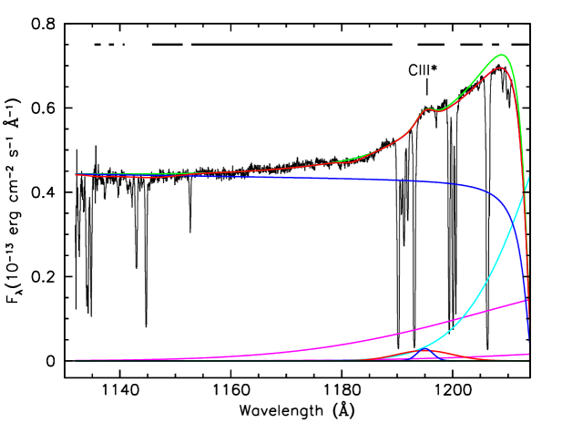
Figure 1: NGC 5548 Mean COS Spectrum, 1130–1214 Å. Best-fit model for the COS UV spectrum of NGC 5548 overlaid on the data (black). The total best-fit model is in red. The model corrected for absorption is in green. (Damped Galactic Ly$\alpha$ is not corrected.) The solid blue line is the continuum component absorbed by damped Galactic Ly$\alpha$. Emission lines from Table 1 are marked. Narrow emission-line region components are in green. Intermediate-line region components are in blue. Broad components are in red. Medium Broad components are in cyan. Very-broad components are in magenta. Thick horizontal bars across the top indicate wavelength intervals used for the fit. Fluxes and wavelengths are in the observed frame.

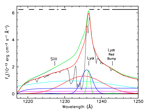
Figure 1: NGC 5548 Mean COS Spectrum, 1217–1250 Å

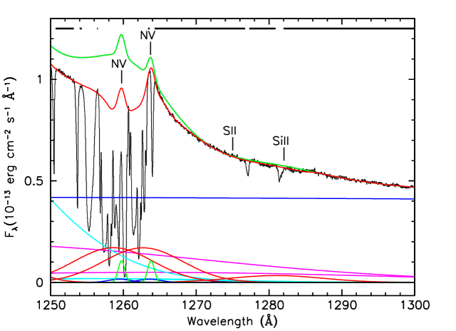
Figure 1: NGC 5548 Mean COS Spectrum, 1250–1300 Å

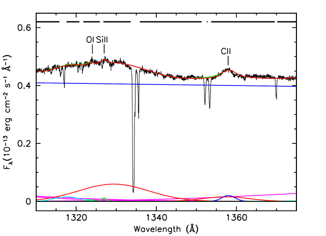
Figure 1: NGC 5548 Mean COS Spectrum, 1310-1375 Å

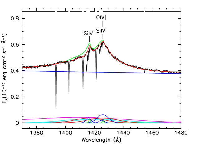
Figure 1: NGC 5548 Mean COS Spectrum, 1370–1480 Å

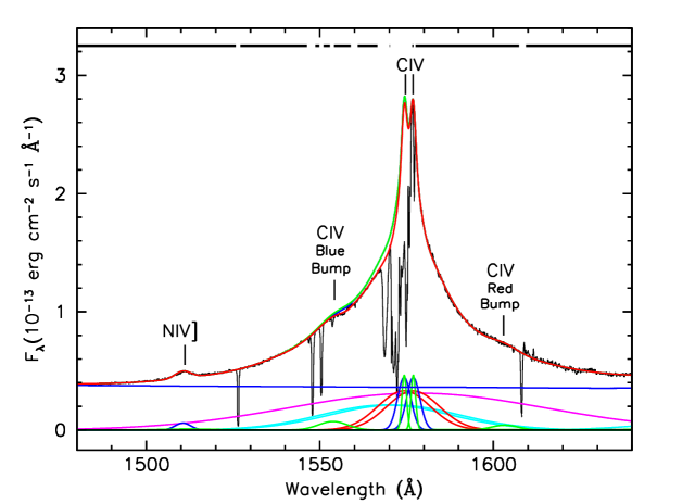
Figure 1: NGC 5548 Mean COS Spectrum, 1480–1640 Å

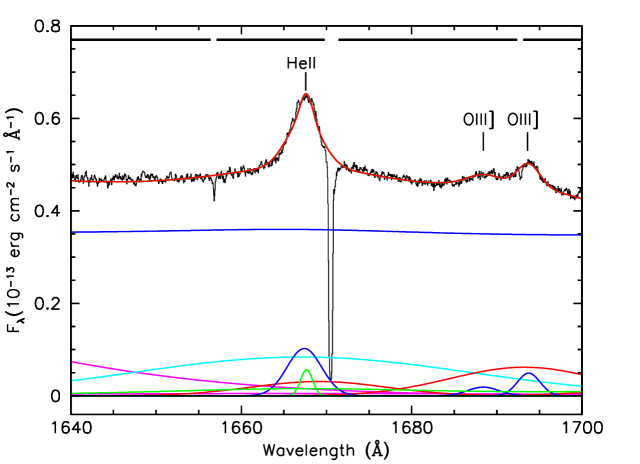
Figure 1: NGC 5548 Mean COS Spectrum, 1640–1700 Å

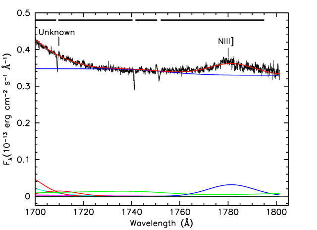
Figure 1: NGC 5548 Mean COS Spectrum, 1700–1805 Å

A final set of empirical emission components in our model accounts for weak bumps on the red and blue wings of C IV and on the red wing of Ly$\alpha$. These bumps have an interesting variability pattern that we discuss later, and they are especially visible in the RMS spectrum shown by De Rosa et al. (2015) in their Figures 1 and 2. We use Gaussian components for each of these features.

We do not model the narrow, intrinsic absorption lines in NGC 5548, nor the foreground interstellar lines, but we do model the variable intrinsic broad absorption associated with the obscurer discovered by Kaastra et al. (2014). The strongest, most easily modeled broad absorption features are on the blue wings of the Ly$\alpha$, N V, Si IV and C IV emission lines. For these, like Kaastra et al. (2014), we use an asymmetric Gaussian with negative flux. To specify the asymmetry we use a larger dispersion on the blue side of the central wavelength than on the red side. We allow the ratio of blue to red dispersion to vary as a free parameter. This parameterization produces a rounded triangular shape with the deepest point in the trough near the red extreme, and a blue wing that extends far out along the blue wing of the emission line. (Kaastra et al. 2014, show these profiles in their Figure 2). We emphasize that this absorption profile is strictly an empirical characterization of the observed flux in the spectrum that has no independent physical meaning. Deriving physical information requires making further assumptions about which emission components are covered, producing a transmission profile, and integrating that profile to obtain the actual opacity. We discuss these measurements later in §3.7.

In addition to these main troughs, additional small depressions appear further out on the blue wings. We model these with additional symmetric Gaussians in negative flux. As with the emission lines, the absorption in N v, Si iv, and C iv is due to doublets. These are unresolved, and we assume they are optically thick. We model each line in the doublet using the same shape and depth. Finally, all the UV resonance lines in the spectrum have weak, blue-shifted absorption troughs at velocities comparable to the main portion of the troughs observed in Ly$\alpha$, N V, Si IV, and C IV. These cannot be modeled in the detail that we apply to the strongest absorption troughs, and they are only readily apparent in the mean spectrum. For these troughs we use symmetric Gaussians in negative flux.

The final component of our model is absorption of all model components by damped Ly$\alpha$ from the Milky Way. We fix the column density at $\rm N(HI)=1.45\times 10^{20}\,{\rm cm}^{-2}$ (Wakker et al. 2011).

Figure 1 gives a detailed view of the best-fit model overlaid on the data. We illustrate all individual components of the model, the best-fit model overlaid on the data, and the absorption-corrected model (which is the ultimate goal of our efforts). Note that the C IV absorption is not as deep in the mean spectrum from the reverberation campaign as it was during the deepest phase of the obscuration as observed in the XMM-Newton campaign of (See Figure S1 in Kaastra et al. 2014, which shows the individual components of the region surrounding the C IV emission line.) For further illustrations of our model of the mean spectrum, see Figures 1 and 2 of De Rosa et al. (2015), which compare the model to the full G130M and G160M spectra.

All the model parameters are listed in Table 1. The model consists of a total of 97 individual components, each with 2–4 parameters. Although the total number of parameters is 383, many of these are fixed, or linked to other parameters. Free parameters in the fit total 143. Although this is a large number, the fit is tightly constrained. The fitted regions in the mean spectrum comprise $\sim 12\,598$ points, each approximately one-half of a resolution element. Thus each spectrum has $\sim 6\,000$ spectral elements included in the fit, and that is described by only 143 parameters.

To optimize the parameters of the model and obtain the best fit, we use a combination of minimization algorithms. After determining initial guesses by visual inspection, we start the optimization process using a simplex algorithm (Murty 1983). This works well for problems with many parameters that are not initially well tuned. Once the fit is nearly optimized, this algorithm generally loses efficiency in approaching full convergence. At that point (usually after several tens of iterations) we switch to a Levenberg-Marquardt algorithm (as originally coded by Bevington 1969). When close to an optimum fit, this algorithm converges rapidly, but with the large number of parameters in our fit, it can get stuck in false minima. To escape these pitfalls, we then alternate sets of 5–10 iterations using the simplex algorithm and the Levenberg-Marquardt algorithm until the fit has fully converged. We define full convergence as $\Delta\chi^{2}<0.01$ and a change in each parameter value of $<$1% after a set of iterations.

3.2 Modeling the Whole Time Series

As we noted above, our Gaussian decomposition of the emission lines is not unique. Therefore, unless one takes care to preserve the overall character of the spectral shape of the model from visit to visit among the individual observations, best fits and parameters can wander far from the character of our fit to the mean spectrum. One could try to avoid this by tailoring initial guesses for fits to each individual spectrum interactively, but this would introduce a unsatisfying degree of subjectivity into our final results. We therefore employed an approach that used quantitative characteristics of the spectra to tune each individual fit and guide it to an optimum result. We verified the soundness of this approach through multiple trials and experiments before converging on a process that produced consistent results from spectrum to spectrum without drastic changes in parameters that might signify unphysical solutions.

In our first trials, we noticed that most weak emission and absorption features were often too weak to be effectively constrained in a single observation. We therefore produced a series of grouped spectra that improved the S/N for our measurements of these weak spectral features. As described in De Rosa et al. (2015), the observations were done in a cycle of 8, where central wavelength settings and FP-POS positions were changed on a daily basis. Combining spectra according to these natural groups produces better S/N, reduces pattern noise, and provides the full spectral coverage that extends down to the P V region at the short wavelength end. In the fits to the time series we discuss below, we use the values for the weak features determined from these grouped spectra as our initial guess for starting parameters when fitting the individual spectra in a group.

Another outcome of our trials, perhaps an obvious one, is that good initial choices for parameters led to quicker convergence and less chance of solutions where parameters strayed into unphysical regions of parameter space. Thus, given our exquisite fit to the mean spectrum, its parameters provide the best guess for spectra that are similar. To strengthen this similarity from fit to fit, we tried two different methods. First, we ordered the spectra by the flux level in the 1367 Å continuum window. We then chose the spectrum near the middle of this distribution with a flux most comparable to the flux in the mean spectrum as the first one to fit. The best fit from this spectrum was then used as the initial guesses for parameters in fitting the next spectra in the series. The series of fits followed two parallel paths moving both higher and lower in flux from this initial middle spectrum. Our second method was to keep the spectra ordered by time, and then pick a spectrum close to the mid-point of the campaign with a mean continuum close to that of the mean spectrum. Fits then progressed both forward and backward in time from this middle point.

These experiments validated our intentions to develop an objective process for determining the best fit to each spectrum. Both methods achieved good fits for all spectra, and the parameters from each method were close in value to each other (typically within the 1-$\sigma$ uncertainties). Figure 2 compares the values obtained as a function of time for the two different methods for three selected parameters from the model. In Figure 2 and in the remainder of the paper, we define times by the Truncated Heliocentric Julian Date (THJD), THJD = HJD $-$ 2400000.

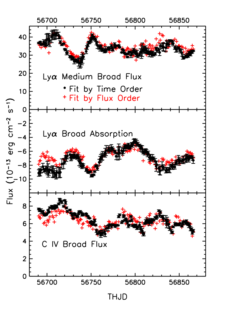
Figure 2: Examples of the evolution of selected parameters comparing values obtained from fits using time-ordered spectra (black points with error bars) to values from fits using flux-ordered spectra (red crosses). Top panel shows the Ly$\alpha$ Medium Broad Flux; the middle panel shows the Ly$\alpha$ Broad Absorption; the bottom panel shows the C IV Broad Flux.

Despite the good agreement in the quality of the fits for the two different methods, our experiments also showed that the second method, “ordered by time”, produced better results than “ordered by flux” in the sense that variations in parameter values were smoother, and, as shown in Figure 3, the best-fit $\chi^{2}$ was typically slightly less. Despite the significant reduction in $\chi^{2}$ we achieved for the fits ordered by time, the differences in the fits are not obvious. We note that for each method $\chi^{2}$ varies systematically with time during the campaign. The variations loosely correspond to the overall variations in brightness of NGC 5548 (as one can see in later figures showing light curves for the continuum and emission line). Our inference for these systematic variations is that the brighter spectra have higher signal-to-noise ratios per pixel, and that subtle residual pattern noise in the flat-field properties of the COS detectors degrade the quality of our fits. Figure 4 compares the best-fit models to the data for two extreme cases, our overall lowest $\chi^{2}$ solution for Visit 38, and our overall highest $\chi^{2}$ obtained for Visit 60. One is hard pressed to see the differences between the models fit using either method, or even why $\chi^{2}$ is significantly higher for Visit 60 compared to Visit 38.

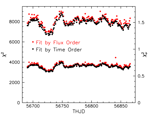
Figure 3: Minimum $\chi^{2}$ achieved in the fit to each spectrum in the campaign (upper curves and left axis). Black points show the results for our adopted method of fitting the sequence of spectra in time order. Red points show the results for fitting the spectra when ordered by flux. Lower curves and the right axis show the reduced $\chi^{2}$. The reduced $\chi^{2}$ is considerably less than one, indicating that our errors are overestimated, likely due to correlated errors, as discussed in §3.4.

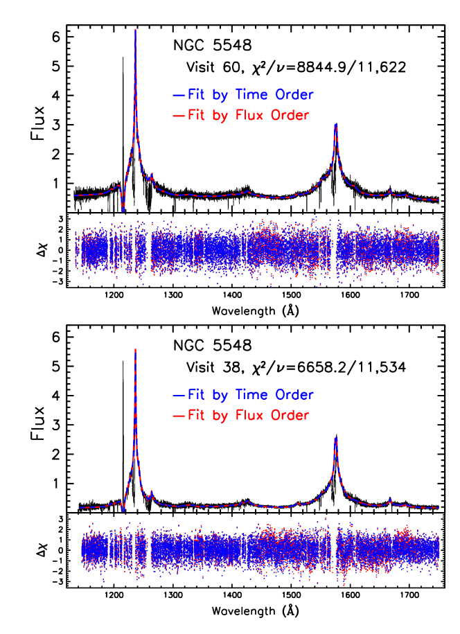
Figure 4: (Top Panel) Best-fit models overplotted on the Visit 60 spectrum. This model has the worst $\chi^{2}$ for the ensemble of fits. The adopted best fit model curve (from fits done in time order) is in blue; the best-fit model for the fits done when ordered by flux is in red. Flux is in the observed frame in units of $10^{-14}~{}\rm erg~{}cm^{-2}~{}s^{-1}~{}\mbox{\AA}^{-1}$. Residuals to the fits are shown as points (”+”) scaled by the 1-$\sigma$ uncertainties, e.g., $\rm\Delta\chi=(Data-Model)/Error$. (Bottom Panel) Same as top panel for the Visit 38 spectrum, which has the best $\chi^{2}$.

Our best inference for why the “ordered by time” sequence produces better results is that the spectrum evolves on timescales of a few days. This is measured in the lags of the emission lines, and, as we will show later in §5.2, it is also true for the absorption features. Therefore, although one spectrum might have the same continuum flux as another, if it is separated in time by more than several days, parameters of major features may differ significantly, making it harder for the minimization algorithm to converge on the best solution.

To fit an individual spectrum, we first determined the best first approximation to the normalization and spectral index of the powerlaw continuum by fitting only those points identified by De Rosa et al. (2015) as continuum windows. To avoid “contaminating” these windows with broad-line flux, we also set the flux of all the Very Broad components to zero. In our experiments, we found that if we did not do this, the Very Broad components developed a tendency to grow in width until they formed their own pseudo-continuum across the whole spectrum. In this first pass, only the powerlaw normalization and the index were allowed to vary freely.

After this step, we then optimized the strength of the brightest emission lines–Ly$\alpha$, N V, Si IV, C IV and He II, and let the fluxes of their Broad and Medium Broad components and the powerlaw normalization vary freely, while keeping the powerlaw index fixed and the Very Broad component turned off. Next, we restored the Very Broad fluxes to their original values, and let the fluxes of all broad components of the above lines vary freely, as well as the powerlaw normalization.

At this point the fit formed a remarkably good representation of an individual observation, but it was still far from the best fit. In the next steps, we turned our attention to optimizing the fits for each individual bright emission line. In these separate steps, we kept all parameters not related to the specific spectral region fixed, including the continuum parameters, the Fe II flux, the Narrow and Intermediate line components for all lines, and any weak blended lines.

For the Ly$\alpha$ region, we did separate optimization steps in this order:

1. Fit Ly$\alpha$ only (Broad, Medium Broad, Very Broad) using only wavelengths 1150–1245 Å. As before, let the fluxes vary freely first, then both the widths and fluxes. Keep all components of N V fixed throughout this.

2. Fit the red wing of N V using only wavelengths 1263–1300 Å. Keep Ly$\alpha$ and all other components fixed. Let the two Broad components vary freely first, then fix them, and let the Medium Broad Components vary. Finally, fix those, and let the Very Broad component vary.

3. Fit the N V absorption on its blue wing, keeping the doublet’s fluxes tied at a 1:1 ratio, using only wavelengths 1245–1264 Å.

4. Free the flux and width of the Broad, Medium Broad, and Very Broad components of Ly$\alpha$.

5. Free the flux and width of the Broad, Medium Broad, and Very Broad components of N V.

6. Free the flux of the Ly$\alpha$ Broad Absorber.

7. Free flux, width, and asymmetry of the Ly$\alpha$ Broad Absorber.

We next did the Si IV region. All parameters that we varied freely above for the optimization of the Ly$\alpha$ region were fixed, and we then:

1. Free the flux of the Broad, Medium Broad, and Very Broad components of Si IV.

2. Free the flux and width of the Broad, Medium Broad, and Very Broad components of Si IV.

3. Free the flux of the Si IV Broad Absorber. (Since the Si IV absorption is so weak, we linked the width and asymmetry of the Si IV Broad Absorber to that of C IV.)

We fit C IV and He II together since they are tightly blended. For optimizing this region, we fix all the previous freely varying parameters, then:

1. Free the flux and width of the Broad, Medium Broad, and Very Broad components of C IV.

2. Free the flux (but not the width) of the Broad, Medium Broad, and Very Broad components of He II.

3. Free the flux of the C IV Broad Absorber.

4. Free the flux, width, and asymmetry of the C IV Broad Absorber.

Once the major emission and absorption components are tuned up, we then allow the weaker emission-line features to adjust. We keep the continuum fixed, as well as all the parameters associated with Ly$\alpha$, N V, Si IV, C IV and He II. The fluxes of all other weak emission features are then allowed to vary.

To complete the optimization, all parameters designated as free to vary in Table 1 are freed, and we iterate the $\chi^{2}$ minimization process until it converges. The best fit parameters for this spectrum are then used as the initial guesses for doing the fit to the next spectrum in the series (with the exception that the initial guesses for the weak features are taken from the best fit to the grouped spectrum corresponding to that spectrum). Final values of all components as a function of wavelength for each spectrum are available as a high-level science product in the Mikulski Archive for Space Telescopes (MAST) as the data set identified by https://doi.org/10.17909/t9-ky1s-j932 (catalog https://doi.org/10.17909/t9-ky1s-j932).

3.3 Propagating the Uncertainties

In principle one can obtain 1-$\sigma$ uncertainties on each of the parameters in our model from the best-fit covariance matrix. However, given the 383 parameters, 143 of which are freely varying, this is computationally impractical. An alternative is to assume that parameter space can be approximated by a parabola near the best-fit minimum in $\chi^{2}$. Using numerically calculated first and second derivatives, one can then extrapolate from the minimum changes in each parameter to achieve $\Delta\chi^{2}=1$, which corresponds to a 1$\sigma$ uncertainty for a single interesting parameter (Bevington 1969). Unfortunately, owing to the high dimensionality of our parameter space and its poor sampling in our calculations, this method proved inadequate.

All the main quantities of interest to be extracted from our models are the fluxes of individual features, either in emission or in absorption. We therefore calculate uncertainties for these quantities using the data and associated uncertainties in each original spectrum, and scaling them in proportion to the quantities that we integrate from our models. To explain this quantitatively, first we define these quantities:
$\rm f_{data,i}=$ flux in pixel $i$ of the original spectrum
$\rm\sigma_{data,i}=$ 1-$\sigma$ uncertainty for pixel $i$ in the original spectrum
$\rm f_{mod,i}=$ flux in pixel $i$ of the modeled spectrum
$\rm\sigma_{mod,i}=$ 1-$\sigma$ uncertainty for pixel $i$ in the model spectrum
$\rm f_{c,j,i}=$ flux in pixel $i$ of the component $j$ (of 97 total)
$\rm\sigma_{c,j}=$ 1-$\sigma$ uncertainty for component $j$.
The flux of the model in pixel $i$ can be decomposed into the sum of the contributions of the individual components:

$$\rm f_{mod,i}=\sum_{j}f_{c,j,i}.$$ (1)

The variance of the model in pixel $i$ is then

$$\sigma_{mod,i}^{2}=\sum_{j}\sigma_{c,j}^{2}.$$ (2)

In the limit of very good statistics, the variance predicted by the model should simply be the variance in the data themselves, i.e.,

$$\sigma_{mod,i}^{2}\sim\sigma_{data,i}^{2},$$ (3)

so the variance in the total flux of any individual component is then

$$\sigma_{c,j}^{2}=\sum_{i}\sigma_{data,i}^{2}\times f_{mod,i}^{2}/(\sum_{k\neq j}f_{c,k,i}^{2}).$$ (4)

If the quantity of interest is the sum of multiple components (i.e., the several components of an emission line contributing to the flux in a given velocity bin), then the 1-$\sigma$ uncertainty we derive for that quantity is

$$\rm\sigma_{tot}=\sqrt{\sum_{j}\sigma_{c,j}^{2}}.$$ (5)

Figure 5 shows the consequences of this method for calculating the 1-$\sigma$ uncertainties. When calculated directly from the data, as described above, the uncertainties are more uniform. The numerical instabilities in our method of interpolating in the error matrix of the fit give uncertainties that largely cluster around the calculation based on the data, but show large excursions, both higher and lower.

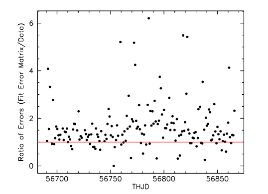
Figure 5: Comparison of uncertainties for the broad Ly$\alpha$ absorption feature in our model. Black points show the ratio of the uncertainty derived from the error matrix of the fit for $\Delta\chi^{2}=1$ divided by the 1-$\sigma$ uncertainty derived as described in §3.3. The ratio scatters about unity (the red line), with large excursions.

3.4 Quality Checking the Fits

The resulting best-fit $\chi^{2}$ for each spectrum is shown as a time series in Figure 3. The number of points in each spectrum varies slightly since the spectrum is moved to multiple positions on the detector using different central wavelength settings. Because of the differing central wavelength settings, not all spectra cover the same range in wavelength as the mean spectrum; the settings tend to lose several hundred points on the blue and red ends of each spectrum. On average, individual spectra have $\sim$11 600 points in each fit. With 143 freely varying parameters, given the $\chi^{2}$ values ranging from $\sim$6800 to $\sim$9000 in Figure 3, one can see that our uncertainties are too large. This is most likely because in aligning and merging each spectrum, we have resampled the original pixels, introducing correlated errors in adjacent bins after rebinning. Note also that $\chi^{2}$ varies systematically with time in the campaign, largely following the light curve of total brightness. A likely explanation for this trend is that it is easier to get a good fit to our complex model when the fluxes are lower and uncertainties are larger.

While the $\chi^{2}$ shows that we have good fits overall, we visually examined each individual fit to see if there were any points or regions where there were systematic deviations of the model from the data. It was these inspections in our early experiments that led us to develop the fitting strategies we documented above. The final fits show no gross or systematic residuals. This is illustrated visually by the image in Figure 6 that shows the residuals of Data$-$Model for each fit stacked into a two-dimensional spectrogram. The only significant features visible are the vertical lines at the positions of interstellar and intrinsic narrow absorption lines, which are not part of our model.

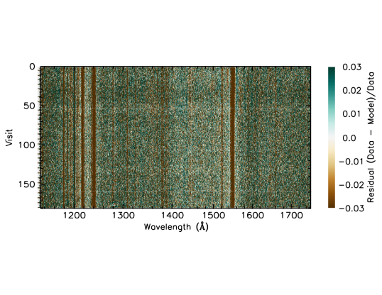
Figure 6: Normalized residuals from the best fit to each spectrum from the campaign. The horizontal axis is in pixels for each spectrum, spanning a wavelength range of 1130–1805 Å. The vertical axis is each individual visit in the campaign.

Our final set of tests compared light curves of fluxes extracted from our model fits to integrations of the same regions of data used in De Rosa et al. (2015). Again here we see no systematic deviations, but these figures do illustrate how the continuum regions are slightly contaminated by wings of the broad emission lines. Figure 7 compares light curves for continuum windows integrated from the raw data, as described by De Rosa et al. (2015), to integrations of the same wavelength regions in our models, both for the full model, and for just the power-law continuum. The lower half of each panel in the figure shows the differences between the two curves along with uncertainties from the raw data. These uncertainties include the systematic repeatability errors described by De Rosa et al. (2015) that apply to the time-series analysis of fluxes from the campaign. These are $\delta_{P}=1.1$% for data with $\lambda<1425$ Å, and $\delta_{P}=1.4$% for $\lambda>1425$ Å. One can see here that the cleanest continuum window, i.e., the one with the least contamination by surrounding emission lines, is the shortest wavelength window surrounding 1158 Å. Although this is the cleanest window in terms of total flux, we use the modeled continuum flux at 1367 Å in our subsequent analysis. Since this is deterministically connected to the modeled flux at 1158 Å through the continuum model, there is no difference between using one or the other.

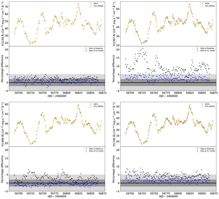
Figure 7: Comparisons of the continuum light curves integrated from the data (green points with error bars) to the fluxes integrated from our best-fit models (gold points with error bars). The top left panel shows the flux at 1158 Å, F(1158 Å), the top right panel F(1367 Å), the bottom left panel F(1469 Å), and the bottom right panel F(1745 Å). The dark gray region in each panel highlights $\pm 2$% errors, and the light gray region shows $\pm 5$% errors.

3.5 The Absorption-corrected Spectra

One of our main goals for these fits to the emission model of each spectrum is to correct for the effects of intrinsic broad absorption, and also to bridge the regions affected by foreground interstellar absorption lines and the narrow intrinsic absorption features in NGC 5548 itself. To correct for the broad absorption, we simply apply the inverse of these model elements to the data. For each pixel corrected in this way, we apply the same scaling to the associated uncertainty as well as the data themselves. To correct for the narrow absorption features (both foreground and intrinsic), since these are not modeled, we replace the data in the wavelength regions affected by the absorption with the emission model.

More specifically, we first visually examined the fit to the mean spectrum to identify points that were significantly affected by narrow absorption lines. These intervals and their identifications are listed in Table 2. Next, we define the following quantities:
$\rm f_{orig}=$ flux in the original spectrum
$\rm f_{mod}=$ flux in the model spectrum (including broad absorption)
$\rm f_{abs}=$ model flux (negative) in the broad absorption lines
$\rm t_{G}=$ transmission profile of Galactic damped Ly$\alpha$
$\rm f_{cor}=$ flux in the corrected spectrum.
The corrected spectrum is then computed in two steps. First, we replace all pixels in the original spectrum with $\rm f_{mod}$ if they fall within the wavelength intervals defined in Table 2. We then compute $\rm f_{cor}=(f_{orig}-f_{abs})/t_{G}$. To calculate the 1-$\sigma$ uncertainties, we scale the original uncertainties in each pixel by the ratio of the corrected flux to the original flux:

$$\rm\sigma_{cor}=\sigma_{orig}\times(f_{cor}/f_{orig}).$$ (6)

3.6 Fluxes in Deblended Emission Lines

With our model fits to the entire series of spectra from the STORM campaign, we can now extract absorption-corrected spectra for all emission lines across their full, deblended velocity profiles. Our models also allow us to separate the variable and non-variable components of the strong emission lines as well as to deblend adjacent lines. For example, Crenshaw et al. (2009) were able to use the faint state of NGC 5548 in 2004 to separate and measure the narrow-line and intermediate-line width components of the Ly$\alpha$ and C IV emission lines. They demonstrated that these components vary only slightly over timescales of years. Using our model, we are able to exclude these non-varying components of the emission lines from the overall broad-line profile. Likewise, we can separate the contributions of blended lines from the wings of Ly$\alpha$ and C IV, and measure lines such as N V as individual species.

For each individual broad emission line, we construct a model profile at each individual pixel $i$ that includes only the contributions of the relevant broad-line components from our model. As described in §3.3, the net flux associated with a given emission feature is

$$\rm f_{totem,i}=\sum_{j}f_{c,j,i},$$ (7)

where the index $j$ runs over all components associated with the desired emission feature. As described in §3.3, we calculate the associated 1-$\sigma$ statistical uncertainty as the fraction in quadrature (relative to all model components in that pixel) of the 1-$\sigma$ uncertainty on the data in that pixel:

$$\rm\sigma_{totem,i}=\sigma_{i}\sqrt{\frac{\sum_{j}f_{c,j,i}^{2}}{\sum_{k}f_{c,k,i}^{2}}},$$ (8)

where the index $j$ runs over all components contributing to the desired emission feature, and the index k runs over all components of the model contributing to the flux in pixel $i$. As described in detail by De Rosa et al. (2015), systematic repeatability errors affect the data when considering time-series analysis of these quantities. We therefore add in quadrature the same errors in precision, namely $\delta_{P}=1.1$% for data from grating G130M ($\lambda<1425$ Å), and $\delta_{P}=1.4$% for data from grating G160M ($\lambda>1425$ Å). These errors in reproducibility actually dominate the uncertainties for all quantities at $\lambda<1180$ Å and $\lambda>1425$ Å.

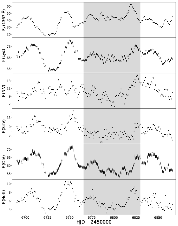
Figure 8: Light curve for the modeled continuum flux at 1367 Å (top panel) in units of $10^{-15}~{}\rm erg~{}cm^{-2}~{}s^{-1}~{}\mbox{\AA}^{-1}$ vs. the Heliocentric Julian Date (HJD) $-$ 2450000. Subsequent panels show light curves for the integrated fluxes of the absorption-corrected deblended emission lines (as labeled) in units of $10^{-13}~{}\rm erg~{}cm^{-2}~{}s^{-1}$. The shaded region shows the time interval of the BLR holiday.

Figure 8 compares light curves for the modeled continuum flux at 1367 Å to the deblended broad emission lines of Ly$\alpha$, N V, Si IV, C IV, and He II. Portions of these light curves are tabulated in Table 3, with full tabulations of these quantities and the other continuum windows (1158 Å, 1430 Å, and 1740 Å) available online. The light curves in Figure 8 closely resemble those derived from the original data shown in Figure 3 of De Rosa et al. (2015). In general, Ly$\alpha$, Si IV and C IV are brighter due to the corrections for absorption, the additional flux from the wings of the very broad emission components, and the elimination of contaminating emission-line flux from the original continuum windows. For He II the flux levels are roughly the same; additional flux from the very broad component of the emission line and a less contaminated continuum are offset by subtraction of blended emission from C IV. Overall, the error bars are smaller since the modeled flux for any given component is determined by many more pixels than the limited wavelength range used in the original integrations. The light curve for N V is a new addition enabled by the deblending from Ly$\alpha$ in our model. In some respects N V differs in character from the other emission lines, especially during the first 75 days of the campaign prior to the BLR holiday. However, starting with the BLR holiday, its behavior is very similar to that of C IV and He II. We will quantify these similarities and differences in §4.1 when we discuss the emission-line lags.

3.7 Measuring the Absorption Lines

The intrinsic narrow absorption lines comprise six discrete velocity components. We adopt the nomenclature of Mathur et al. (1999), numbering each component in order starting at the highest blue-shifted velocity. To illustrate this kinematic structure, Figure 9 shows normalized absorption profiles for the most prominent intrinsic absorption lines as a function of velocity relative to the systemic velocity of the host galaxy NGC 5548. For this we adopt the H I 21-cm redshift of $z=0.017175$ (de Vaucouleurs et al. 1991).

Measuring the strengths of the intrinsic narrow absorption lines is straightforward. Using the complete model of each spectrum (including the broad absorption components, since they help define the local continuum surrounding the narrow intrinsic absorption lines), we measure the equivalent widths by integrating across each absorption-line profile in the normalized spectrum. These integrations are performed as discrete sums over pixels lying within the wavelength regions defined for each feature in Table 4:

$$EW=\sum_{i}(f_{orig,i}-f_{mod,i})/f_{mod,i}\times\Delta\lambda.$$ (9)

The 1-$\sigma$ uncertainty for EW is obtained by simply propagating the uncertainty associated with each data point in the original spectrum used in the sum:

$$\sigma_{EW}=\sqrt{\sum_{i}(\sigma_{orig,i}^{2}/f_{orig,i}^{2})\times\Delta\lambda^{2}}.$$ (10)

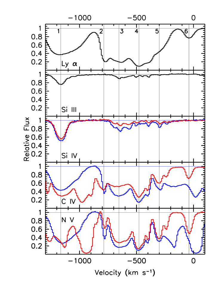
Figure 9: Intrinsic narrow absorption features in NGC 5548. Normalized relative fluxes are plotted as a function of velocity relative to the systemic redshift of $z=0.017175$. The top panel shows Ly$\alpha$, the second panel Si III $\lambda 1206$, the third panel Si IV $\lambda 1393$ (blue) and Si IV $\lambda 1402$ (red), the fourth panel C IV $\lambda 1548$ (blue) and C IV $\lambda 1550$ (red), and the bottom panel N V $\lambda 1238$ (blue) and N V $\lambda 1242$ (red). Thin vertical lines indicate the velocities of the six intrinsic absorbers.

We take caution in performing these integrations to avoid features blended with Galactic absorption lines, or with other transitions. For example, the close velocity spacings of the C IV and N V doublets ($498~{}\rm km~{}s^{-1}$ and $964~{}\rm km~{}s^{-1}$, respectively) cause components #1, #2, #3, and #5 in C IV to overlap, and Components #1 and #5 in N V to overlap, as shown in Figure 10. The red transition of Component #1 in the N V doublet is blended with Galactic S II$\lambda 1259$, and the blue transition of Component #6 is blended with Si II$\lambda 1260$. Therefore Table 4 gives measurements only for clean, unblended features.

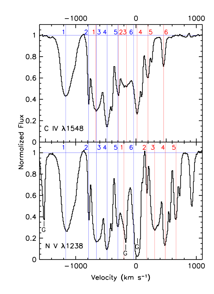
Figure 10: Illustration of blending in the absorption lines of the C IV and N V doublets in NGC 5548. Normalized relative fluxes are plotted as a function of velocity relative to the systemic redshift of $z=0.017175$. The top panel shows C IV $\lambda 1548$, and the bottom panel N V $\lambda 1238$. Thin vertical blue lines indicate the velocities of the blue components of the doublets for the six intrinsic absorbers. Vertical red lines show the locations of the corresponding red components. Foreground Galactic interstellar absorption lines are marked with a “G”.

The equivalent width of each broad absorption feature (EW) is calculated from the normalized modeled spectrum,

$$\rm f_{norm,i}=f_{mod,i}/(f_{mod,i}-f_{abs,i}),$$ (11)

as

$$EW=\sum_{i}(1-f_{norm,i})\times(\lambda_{i+1}-\lambda_{i}),$$ (12)

where $\lambda_{i}$ is the wavelength of pixel $i$. Since our spectra are linearized, $\Delta\lambda=\lambda_{i+1}-\lambda_{i}$, is actually a constant. The corresponding 1-$\sigma$ uncertainty is

$$\rm\sigma_{EW}=(f_{totabs}/EW)\times\sigma_{totabs},$$ (13)

where $f_{totabs}$ and $\sigma_{totabs}$ are defined below.

The broad UV absorption troughs associated with the obscurer in NGC 5548 are shown in Figure 2 of Kaastra et al. (2014). These broad troughs are asymmetric, and they extend from near zero velocity in the systemic frame of the host galaxy to $\sim-5500~{}\rm km~{}s^{-1}$. The time-varying strengths of the intrinsic broad absorption lines in NGC 5548 that are associated with the obscurer are part of the models we have fit to all the spectra. These all have one main component, but there are also weaker components on the high-velocity blue wing of the absorption profile. These individual weak components are often not well constrained by the model fits. We therefore calculate the total absorption, $\rm f_{totabs}$ for the sum of all components associated with a given spectral transition. The total flux is then

$$\rm f_{totabs}=\sum_{j}f_{c,j},$$ (14)

where the index $j$ runs over all components associated with the desired line, and the associated uncertainty is calculated as the quadrature sum of the 1-$\sigma$ uncertainties of each component $j$:

$$\rm\sigma_{totabs}=\sqrt{\sum_{j}\sigma_{c,j}^{2}}.$$ (15)

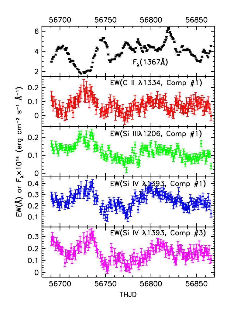
Figure 11: (Top Panel) Light curve for the UV continuum at 1367 Å in units of $10^{-14}~{}\rm erg~{}cm^{-2}~{}s^{-1}~{}{\mbox{\AA}}^{-1}$. Lower panels show the absolute value of the equivalent width in Å vs. time for selected absorption lines. (Second Panel) C II $\lambda 1334$, narrow absorption Component #1. (Third Panel) Si III $\lambda 1206$, narrow absorption Component #1. (Fourth Panel) Si IV $\lambda 1393$, narrow absorption Component #1. (Bottom Panel) Si IV $\lambda 1393$, narrow absorption Component #3.

Table 5 shows sample portions of the light curves for the broad absorption in C IV and the intrinsic narrow absorption associated with C II $\lambda 1334$. Full light curves for all features listed in Table 4 are published in the on-line version of this paper. Figure 11 shows sample light curves for the equivalent widths of the narrow absorption features associated with Component #1 for C II $\lambda 1334$, Si III $\lambda 1206$, and Si IV $\lambda 1393$, plus Component #3 for Si IV $\lambda 1393$, all compared to the UV continuum flux at 1367 Å. Light curves for the broad absorption in C IV, N V, Ly$\alpha$, and Si IV are shown in Figure 12.

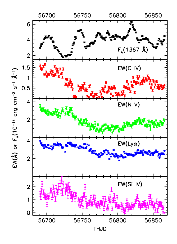
Figure 12: (Top Panel) Light curve for the UV continuum at 1367 Å in units of $10^{-14}~{}\rm erg~{}cm^{-2}~{}s^{-1}~{}\mbox{\AA}^{-1}$. (Second Panel) Absolute value of the equivalent width in Å vs. time for the broad C IV absorption feature. (Third Panel) Same as second panel for N V. (Fourth Panel) Same as second panel for Ly$\alpha$. (Bottom Panel) Same as second panel for Si IV.

4 Analyzing Results from the Models

4.1 Velocity Resolved Light Curves for Deblended Emission Lines

Our absorption-corrected, deblended emission line profiles described in §3.6 allow us to remove the uncertainties in emission-line lags that may have been introduced by the variable intrinsic absorption in NGC 5548, as well as to separate the behaviors of adjacent blended lines. In addition, for the brightest two lines, Ly$\alpha$ and C IV, we can determine velocity-binned lags for each line uncontaminated by absorption or blended contributions from other lines.

Following De Rosa et al. (2015) we measured the emission-line lags for the species tabulated in Table 3 by cross-correlating the time series with the continuum light curve using the interpolation cross-correlation method (ICCF) as implemented by Peterson et al. (2004). The procedure and the resulting associated uncertainties are described in detail by De Rosa et al. (2015). Briefly, the technique uses a Monte-Carlo method of “flux randomization and random subset selection” to generate a large set of realizations of the light curves. For each realization, we determine the cross correlation function, its maximum correlation coefficient $r_{max}$, and associated peak lag, $\tau_{peak}$. We also use the region surrounding the peak with $r(\tau)>0.8$ to calculate the centroid of the cross-correlation function, $\tau_{cent}$. A few thousand realizations of each cross-correlation function then gives distribution functions for $\tau_{peak}$ and $\tau_{cent}$ from which we measure the median values to give the lags for each emission line as presented in Table 6. The associated uncertainties represent the 68% confidence intervals of each Monte-Carlo distribution.

While De Rosa et al. (2015) arbitrarily split the data set in two midway through the campaign, we now know that a more logical breakpoint for examining any changes is at day 75 in the campaign, which is the beginning of the period when the broad emission line fluxes become decorrelated from the continuum variations (Goad et al. 2016), also known as the BLR holiday. We therefore quote lags not only for the full campaign, but also for the first 75 days, the pre-holiday period, when the emission line and continuum fluxes correlated normally; for the holiday period, days 76–129; and for the post-holiday period at the end of the campaign. Comparing the lags in Table 6 to De Rosa et al. (2015), we see that Ly$\alpha$ is slightly shorter, Si IV is longer, and C IV and He II are about the same. Within the error bars, the lags for the UV model data set are consistent with the prior results using the original data.

Table 6: Emission-Line Lags from the Modeled NGC 5548 Spectra

Emission Line	Ly$\alpha$	N V	Si IV	C IV	He II
Whole Campaign–Modeled Data
$\tau_{\rm cent}$	5.1$\pm$0.3	7$\pm$8	8.1$\pm$0.7	5.8$\pm$0.5	2.2$\pm$0.3
$\tau_{\rm peak}$	5.1$\pm$0.6	6$\pm$7	8.1$\pm$1.0	5.7$\pm$0.6	1.9$\pm$0.4
$r_{\rm peak}$	0.71$\pm$0.03	0.17$\pm$0.06	0.16$\pm$0.04	0.39$\pm$0.04	0.56$\pm$0.03
Pre-BLR Holiday, THJD=56691–56765
$\tau_{\rm cent}$	4.8$\pm$0.3	…	8.0$\pm$0.5	4.4$\pm$0.3	2.4$\pm$0.4
$\tau_{\rm peak}$	4.8$\pm$0.4	…	8.1$\pm$0.6	4.5$\pm$0.5	2.2$\pm$0.4
$r_{\rm peak}$	0.94$\pm$0.01	…	0.7$\pm$0.04	0.91$\pm$0.02	0.91$\pm$0.02
BLR Holiday, THJD=56766–56829
$\tau_{\rm cent}$	5$\pm$1	4.5$\pm$0.4	7.3$\pm$1	7.1$\pm$0.6	2.1$\pm$0.4
$\tau_{\rm peak}$	5$\pm$1	4.4$\pm$0.6	7.3$\pm$1	7.3$\pm$0.7	2.1$\pm$0.5
$r_{\rm peak}$	0.74$\pm$0.06	0.79$\pm$0.04	0.66$\pm$0.06	0.73$\pm$0.07	0.75$\pm$0.05
Post-BLR Holiday, THJD=56830–56866
$\tau_{\rm cent}$	6$\pm$1	5$\pm$3	10$\pm$2	8$\pm$1	7$\pm$5
$\tau_{\rm peak}$	7$\pm$1	2${}^{+1}_{-4}$	10$\pm$3	8.5$\pm$2.2	10${}^{+1}_{-8}$
$r_{\rm peak}$	0.85$\pm$0.04	0.72$\pm$0.06	0.77$\pm$0.19	0.80$\pm$0.13	0.63$\pm$0.09
Whole Campaign–Original Data
$\tau_{\rm cent}$	6.2$\pm$0.3	…	5.3$\pm$0.7	5.3$\pm$0.5	2.5$\pm$0.3
$\tau_{\rm peak}$	6.1$\pm$0.4	…	5.4$\pm$1.1	5.2$\pm$0.7	2.4$\pm$0.6
$r_{\rm peak}$	0.77$\pm$0.02	…	0.46$\pm$0.06	0.36$\pm$0.04	0.65$\pm$0.03
Pre-BLR Holiday, THJD=56691–56765
$\tau_{\rm cent}$	5.8$\pm$0.3	…	5.2$\pm$0.8	4.3$\pm$0.3	2.4$\pm$0.4
$\tau_{\rm peak}$	5.9$\pm$0.4	…	5$\pm$1	4.4$\pm$0.5	1.4${}^{+0.9}_{-0.1}$
$r_{\rm peak}$	0.94$\pm$0.01	…	0.7$\pm$0.04	0.93$\pm$0.02	0.90$\pm$0.02
BLR Holiday, THJD=56766–56829
$\tau_{\rm cent}$	5.2$\pm$0.6	…	6$\pm$2	6.9$\pm$0.9	3.3$\pm$0.6
$\tau_{\rm peak}$	5${}^{+1}_{-0.4}$	…	6$\pm$2	7$\pm$1	3.3$\pm$0.8
$r_{\rm peak}$	0.84$\pm$0.04	…	0.52$\pm$0.09	0.64$\pm$0.09	0.74$\pm$0.06
Post-BLR Holiday, THJD=56830–56866
$\tau_{\rm cent}$	7$\pm$1	…	7$\pm$1	8$\pm$1	3$\pm$1
$\tau_{\rm peak}$	8$\pm$2	…	7$\pm$2	8$\pm$2	3$\pm$1
$r_{\rm peak}$	0.83$\pm$0.08	…	0.75$\pm$0.11	0.82$\pm$0.12	0.81$\pm$0.05

Note. — Delays measured in days in the rest frame of NGC 5548.

Comparing results for the different time intervals within the campaign reveals an interesting evolution in the emission-line lags. As expected, during the pre-holiday period when the emission-line fluxes correlated well with the continuum fluctuations, correlation coefficients are high, exceeding $r=0.9$ for Ly$\alpha$, C IV and He II. For N V, however, the correlation is so poor that we cannot determine a lag in the pre-holiday period, as expected from the lack of any strong features in this region of the light curve in Figure 8. During the holiday period, correlation coefficients are lower, but they are still very good, with $r>0.65$ for all lines. Lags for all lines during the holiday are about the same as for the pre-holiday period except for C IV. The C IV lag during the holiday is significantly longer than for the pre-holiday period by almost three days. In the post-holiday period, correlation coefficients are again very good, and C IV shows significantly longer lags compared to the pre-holiday period. Other lines hint at such a difference, but not significantly. These changing lags with time explain why the correlation coefficients for the overall campaign are low despite the much longer data set. Together with changes in the velocity-resolved lags discussed below, this may indicate that significant changes in the structure (or at least our viewpoint) or the illumination, or both, of the BLR are occurring on the timescale of our campaign. Given that the orbital timescale at a radius of 1 light day in NGC 5548 is 115 days, such changes seem plausible.

To ensure that this apparent increase in the emission-line lags over the course of the campaign is not an artifact of our modeling of the data, we reanalyzed the original data of De Rosa et al. (2015) by splitting it into the same time intervals. The results are given in the bottom half of Table 6. The lags for the whole campaign replicate the original results of De Rosa et al. (2015), and we see the same lengthening of lags toward the end of the campaign with similar values to those found using the modeled data.

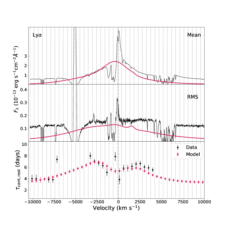
Figure 13: (Top panel) Comparison of the mean spectrum in the Ly$\alpha$ region of NGC 5548 (black data curve) to the best-fit model spectrum corrected for absorption with the continuum subtracted and narrow and intermediate emission-line components removed (smooth red curve). (Middle panel) Same as top panel for the RMS spectrum. (Bottom Panel) We compare velocity-binned centroids from the interpolated cross-correlation function across the Ly$\alpha$ profile obtained using the original data (black dots) to the absorption-corrected model with narrow and intermediate emission-line components removed (red squares). Lags are in the rest frame of NGC 5548.

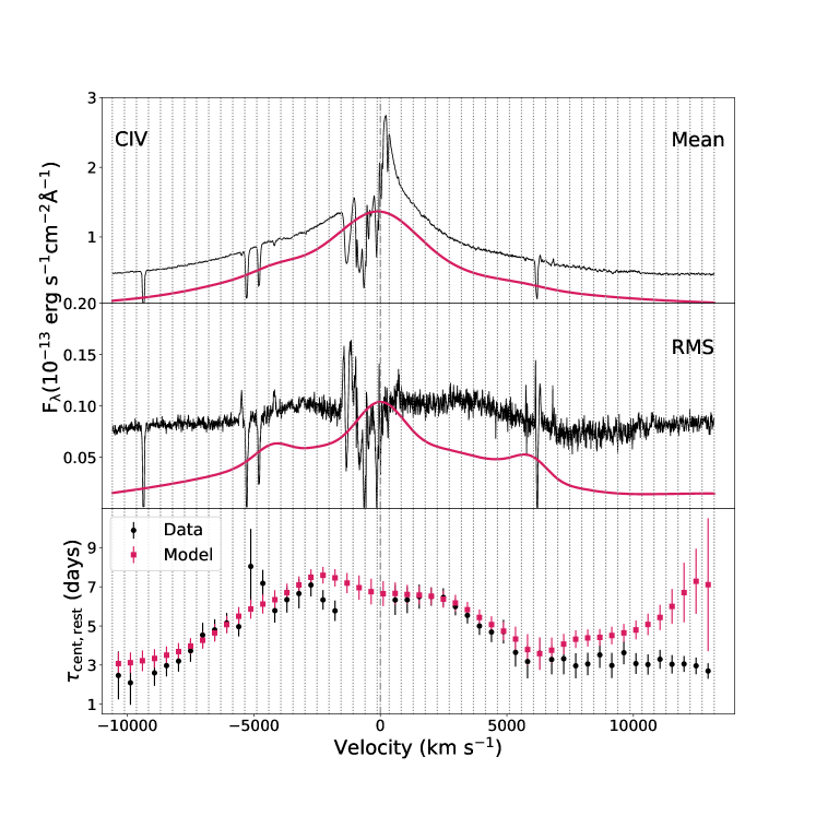
Figure 14: Same as 13, but for C IV.

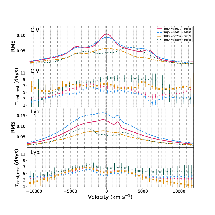
Figure 15: (Top panel) Comparison of the RMS spectra in the C IV emission-line region of NGC 5548 for four different time intervals. All curves refer to the modeled UV spectrum as corrected for absorption with the continuum subtracted and narrow and intermediate emission-line components removed. The smooth red curve is for the full campaign, THJD = 56691–56866. The dotted blue curve is for the first 75 days of the campaign, the pre-holiday period, THJD = 56691–56765. The dash-dot gold curve is for the period of the BLR holiday, THJD = 56766–56829. The dotted green curve is for the post-holiday period, THJD = 56830–56866. (Second panel) We compare velocity-binned centroids from the interpolated cross-correlation function across the absorption-corrected model for C IV with narrow and intermediate emission-line components removed. Lags are in the rest frame of NGC 5548. Red triangles show results for the full campaign, THJD = 56691–56860. Blue triangles are for the first 75 days of the campaign, the pre-holiday period, THJD = 56691–56765. Gold squares are for the period of the BLR holiday, THJD = 56765–56829. Green crosses are for the post-holiday period, THJD = 56830–56866. (Third panel) Same as top panel, but for the Ly$\alpha$ emission line. (Bottom Panel) Same as second panel, but for the Ly$\alpha$ emission line.

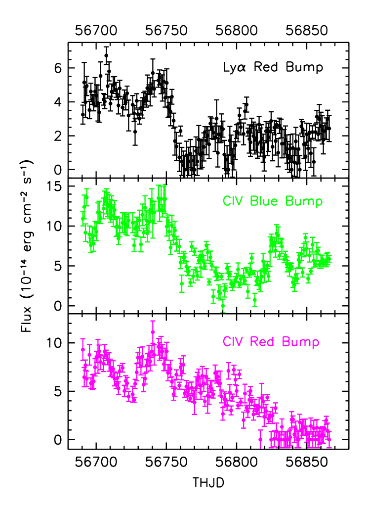
Figure 16: (Top Panel) Light curve (points in black with 1-$\sigma$ error bars) for the flux in the emission bump on the red wing of Ly$\alpha$ at $\sim+1500~{}{\rm km~{}s^{-1}}$. (Middle Panel) Same for the emission bump on the blue wing of C IV at $\sim-4300~{}{\rm km~{}s^{-1}}$ (green). (Bottom Panel) Same for the emission bump on the red wing of C IV at $\sim+5700~{}{\rm km~{}s^{-1}}$ (magenta). Fluxes are in units of of $10^{-14}~{}\rm erg~{}cm^{-2}~{}s^{-1}$.

Also interesting are the velocity-binned results for Ly$\alpha$ and C IV. Absorption in NGC 5548 largely obscured the inner few thousand $\rm km~{}s^{-1}$ of the blue side of the profile of each emission line, and N V or He II emission contaminated the far red wings. Following De Rosa et al. (2015), we use bins of $500~{}\rm km~{}s^{-1}$ spanning each profile. Figure 13 compares the mean spectrum for the modeled broad component of Ly$\alpha$, its corresponding root-mean-square (RMS) spectrum, and finally the velocity-binned profile to the original data from De Rosa et al. (2015). All data are for the full campaign. Our modeled profile provides full velocity coverage across the Ly$\alpha$ emission line. The most noticeable characteristic of the lag profile is its distinct “M” shape, with a local minimum in the lag near zero velocity, and maxima on the red and blue sides at $\pm 2500~{}\rm km~{}s^{-1}$. A prominent feature in the RMS spectrum is the “red bump” on the Ly$\alpha$ emission-line profile at $+1500~{}\rm km~{}s^{-1}$, which loosely corresponds to the local peak in the the velocity-dependent lag profile on the red wing of Ly$\alpha$.

Figure 14 shows the corresponding set of results for the C IV emission line. For C IV there are emission bumps on both the red and blue wings of the profile in the RMS spectrum. These bumps are at higher velocity than the red bump in Ly$\alpha$, at roughly $\pm 5000~{}\rm km~{}s^{-1}$, and they appear to correspond to local minima in the lag profile, as opposed to the maxima seen in Ly$\alpha$. As with Ly$\alpha$, C IV shows a slight hint of an “M” shape to its profile with a shorter lag near the center and local peaks at $\pm 2500~{}\rm km~{}s^{-1}$. However, the contrast is not as distinctive as in Ly$\alpha$. The central dip in C IV has a confidence level of only $\sim 90$%.

Examining the velocity-binned profiles for the separate, distinct time intervals of the campaign reveals even more complex behavior. Figure 15 compares the RMS spectra and the velocity-dependent lags for C IV and Ly$\alpha$ from the full campaign to the first 75 days of the campaign, the pre-holiday period, the period of the BLR holiday, and the post-holiday period concluding the campaign. The emission bumps on the red and blue wings of C IV and on the red wing of Ly$\alpha$ are most prominent early in the campaign, and diminish in flux (or, disappear in the case of C IV red) by the end of the campaign. We show light curves for these features in Figure 16. The red emission bump in C IV also has associated features in the lag profiles that evolve from a local minimum on the red side of the bump during the pre-holiday period to a local maximum in the lag on the blue side of the bump. These more detailed changes in the emissivity profile and the lag profile again suggest that we are seeing changes in the structure of the BLR over the course of the campaign. This may be due to the presence of some outflowing components, as discussed in §5, but this is speculative, and more easily investigated with two-dimensional reverberation maps and models.

4.2 Physical Characteristics of the Narrow and Broad Absorbers based on the Mean Spectrum

The very high S/N of the mean spectrum makes accurate measures of weak features possible. These are particularly useful since they are often unsaturated, and can therefore provide better diagnostic information on physical conditions in the absorbing gas. The last four columns of Table 4 give the EW, the velocity relative to the systemic velocity of the host galaxy, the covering factor, and the inferred column density for the narrow absorption lines in the mean spectrum. For Galactic ISM features, the inferred column densities are at best lower limits since the lines are saturated, and since the profiles have not been corrected for the COS line spread function. For absorption lines intrinsic to NGC 5548, the line widths are broad enough (FWHM typically $>80~{}\rm km~{}s^{-1}$) that the COS line spread function has little effect. To measure column densities, we integrate the apparent optical depth across the absorption line profile between the wavelength limits given in Table 4, assuming a uniform covering factor, as given in the next-to-last column of the table (see Appendix A of Arav et al. 2015, for a description of the technique). For doublets and for absorption lines with multiple transitions (e.g., P V, or Si II), we can determine the covering factor such that integration of each line profile gives consistent column densities. For other absorption lines, particularly the deep, heavily blended features associated with Ly$\alpha$, N V, and C IV, we use a covering factor determined by the deepest point of the absorption-line profile and assume the line is saturated. Like Arav et al. (2015), this gives a lower limit on the column density.

Examining the covering factors in Table 4 is instructive. Lines far from the centers of the bright emission lines (e.g., P V, Si II $\lambda 1302$, C II $\lambda 1335$) have covering factors near unity, indicating that the absorbing gas fully covers, or nearly fully covers, the continuum emission region. These absorption lines are also multiplets, so their covering factors are well determined. Other absorption lines embedded in the profiles of bright emission lines such as (C III* $\lambda 1176$, Si II $\lambda 1193$, and Si II $\lambda 1260$), have well determined covering factors that are significantly less than unity, and vary depending on their distance from the center of the emission line. The sense of this variation is such that covering factors are lower for lines in the brighter portions of the emission line profile. From this we conclude that, at least for Component #1, the absorbing gas nearly fully covers the continuum-emitting region, but only covers less than half of the BLR.

The column densities in Table 4 for the STORM campaign mean spectrum are factors of several lower than those observed by Arav et al. (2015) during the XMM-Newton campaign. This is consistent with the higher brightness of NGC 5548 during the STORM campaign— $\rm\langle F_{\lambda 1367}\rangle=4.30\times 10^{-14}~{}erg~{}cm^{-2}~{}s^{-1}~{}\mbox{\AA}^{-1}$ vs. $\rm\langle F_{\lambda 1367}\rangle=3.11\times 10^{-14}~{}erg~{}cm^{-2}~{}s^{-1}~{}\mbox{\AA}^{-1}$. Simple scaling of the continuum would imply an increase in the ionization parameter of $\Delta\rm log$ $U$ of 0.14. Although this seems small, it is sufficient to account for the observed differences since the weak, low-ionization species in Component #1 are formed in a thin hydrogen ionization front, and their column densities are highly non-linear with changes in ionizing flux.

We tabulate the properties of the broad absorption features separately since these are most likely associated with the soft X-ray obscurer discovered by Kaastra et al. (2014). To obtain the equivalent width (EW), the mean transmission-weighted velocity, the transmission-weighted velocity dispersion, and the column density of each broad absorption trough, we use the normalized mean spectrum of NGC 5548. For each trough we use the highest blue-shifted velocity at which the trough drops by more than $1\sigma$ below the normalized spectrum. All troughs are integrated up to zero velocity. Since these broad troughs are well resolved, we use the apparent optical depth method of Savage & Sembach (1991) to calculate the column densities of each trough. The deepest absorption troughs in N V, Si IV, and C IV appear to be saturated since they have similar depths at the velocities of the red and blue members of their respective doublets. Since Ly$\alpha$ is of similar depth, we also assume it is saturated. We therefore measure a covering factor $\rm C_{f}$ at the deepest point of the trough and use this in our apparent optical depth calculation (Arav et al. 2002). This column density is only a lower limit to the actual column density. The shallower absorption troughs are significantly less deep. If they were saturated and had similar covering factors, they would likely have similar depths to those of the stronger ions. We therefore assume that they lie on the linear portion of the curve of growth and use their apparent optical depths to obtain a direct measure of the column density assuming covering factors of unity. Table 7 summarizes the broad absorption trough properties in detail.

Table 7: Properties of the Broad Absorption Troughs in the NGC 5548 Mean Spectrum

Line	$\lambda_{o}$	$v_{1}$	$v_{2}$	$v_{o}$	$\sigma_{v}$	EW	$\rm log(N_{ion})$	$\rm C_{f}$
	(Å)	($\rm km~{}s^{-1}$)	($\rm km~{}s^{-1}$)	($\rm km~{}s^{-1}$)	($\rm km~{}s^{-1}$)	(Å)	($\rm cm^{-2}$)
P V	1122.99	$-1388$	0	$-\phantom{0}751$	$\phantom{0}726$	$0.07\pm 0.04$	$13.11\pm 0.03$	1.0
C III*	1175.8	$-5323$	0	$-1250$	$1054$	$0.06\pm 0.01$	$12.72\pm 0.07$	1.0
Ly$\alpha$	1215.67	$-6344$	0	$-1931$	$1160$	$2.95\pm 0.02$	$>14.80$	0.25
N V	1240.51	$-4907$	0	$-1697$	$1054$	$1.70\pm 0.02$	$>14.81$	0.17
Si II	1260.42	$-7894$	0	$-4592$	$\phantom{0}986$	$0.09\pm 0.01$	$12.80\pm 0.05$	1.0
C II	1334.53	$-2067$	0	$-\phantom{0}953$	$\phantom{0}439$	$0.04\pm 0.01$	$12.96\pm 0.09$	1.0
Si IV	1398.27	$-4913$	0	$-1878$	$1005$	$0.84\pm 0.02$	$>13.83$	0.06
C IV	1549.48	$-4627$	0	$-1893$	$1091$	$0.63\pm 0.01$	$>14.02$	0.07

We can now use these measures of ionic column densities in the UV together with the X-ray opacity measurements from the XMM-Newton spectra of Kaastra et al. (2014) to determine the ionization state of the obscurer more accurately. Because of the low X-ray flux resulting from the heavy X-ray absorption, the XMM-Newton spectra have no detectable spectral features that we can use to determine the ionization properties of the obscurer. However, the X-ray spectrum does provide a good measure of the total column density. As in the study of the obscurer in NGC 3783 (Kriss et al. 2019), we examine joint photoionization models that use the UV ionic column densities along with the total column density determined from the X-ray observations to more precisely determine the physical properties of the obscurer. Since the obscuring gas is illuminated by the bare active nucleus in NGC 5548, we use the unobscured spectral energy distribution (SED) shown in Figure 2 of Arav et al. (2015) for our photoionization models. Using Cloudy v17.00 (Ferland et al. 2017), we run a grid of models covering a range of $-1.5$ to 2.0 in ionization parameter log $\xi$, and total column densities from log $\rm N_{H}=21.0$ to 23.5. Figure 17 shows the allowed space of photoionization solutions, which are at the two points where the X-ray column densities of the two obscurer components intersect the measured column densities of C II, C III*, Si II, and P V in the grid of photoionization models. Note that no single solution fits all measured ions, but some of this incommensurability could be due to the unknown covering fraction of the weak, low-ionization species. In addition, all these low-ionization species are produced in very narrow ionization fronts, so there are likely systematic errors in the photoionization modeling (see Mehdipour et al. 2016a) that are larger than the statistical uncertainties we show in the figure. Kaastra et al. (2014) used only the XMM-Newton X-ray spectra to determine the ionization parameter and column density of the obscurer, Since there are no spectral features to constrain the X-ray models, a broad range of ionization parameters produces acceptable fits. As shown by Mehdipour et al. (2017), Kriss et al. (2019) and Longinotti et al. (2019), including the UV absorption as an additional constraint indicates that the obscuring gas likely has higher ionization, even in the observations of the original XMM-Newton campaign. From our new analysis that includes the broad UV absorption as part of the solution, we see that the obscurer is much more highly ionized than originally thought. Component #1, with $\rm log~{}N_{H}~{}cm^{-2}=22.08$ actually has an ionization parameter in the range $\rm log~{}\xi_{1}=0.8$–0.95, and Component #2 is even more highly ionized at $\rm log~{}\xi_{2}=1.5$–1.6. These differ sufficiently from the original fits of Kaastra et al. (2014) ($\rm log~{}\xi_{1}=-0.8$ and $\rm log~{}\xi_{2}=-4.5$) that another look at the X-ray spectral analysis is warranted.

4.3 Variability of the Narrow Absorption Features

The narrow intrinsic absorption features in NGC 5548 lie at distances of $\sim 3$ to hundreds of parsecs (Arav et al. 2015). They vary on timescales of days (as seen above in Figure 11) to years (Arav et al. 2015), and appear to be associated with the X-ray warm absorber in NGC 5548 (Mathur et al. 1995; Crenshaw et al. 2009; Kaastra et al. 2014; Arav et al. 2015). Using density sensitive transitions in the metastable excited states of C III and Si III, Arav et al. (2015) determined the density of the gas producing the absorption features associated with Component #1 as $\rm log~{}n~{}cm^{-3}=5.8\pm 0.3$, placing it at a distance of $3.5\pm 1.0$ pc, consistent with the density and the 1–3 pc location of the emission-line gas in the NLR (Peterson et al. 2013). Using the time variability of these absorption features, we can independently measure the density by measuring the recombination time in the gas. Krongold et al. (2007) used the variability of the aggregate soft X-ray absorption as it responded to continuum flux changes in NGC 4051 to estimate recombination times, but here we have the opportunity to make such measurements with distinct, resolved, absorption lines in the UV.

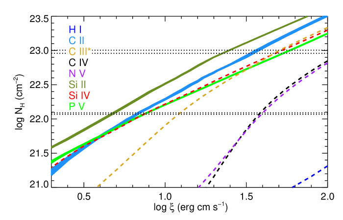
Figure 17: Photoionization model constraints on the obscurer in NGC 5548. Dotted black lines give the range of total column density for the two components of the obscurer (Kaastra et al. 2014). Thick colored bands show the column densities with associated 1-$\sigma$ uncertainties for the weak, low-ionization troughs in the mean UV spectrum of NGC 5548. Nominally, photoionization solutions should lie along these lines. For the strong, saturated features, we use dashed colored lines for the lower limits on their column densities. Allowed photoionization solutions lie above these lines.

For gas in photoionization equilibrium, the population density $n_{i}$, in a state $i$ depends on the balance between the ionizing photon flux causing ionizations to more highly ionized states and recombinations from those states. Following Krolik & Kriss (1995), this can be expressed as

$$dn_{i}/dt=-(F_{ion,i}\sigma_{ion,i}+n_{e}\alpha_{rec,i-1})n_{i}$$ (16)

$$\phantom{0000000000}+n_{e}n_{i+1}\alpha_{rec,i}+F_{ion,i-1}\sigma_{ion,i-1}n_{i-1}.$$

For the ions we are measuring, generally $n_{i-1}\ll n_{i}\ll n_{i+1}$, so we can simplify to

$$dn_{i}/dt=-F_{ion,i}\sigma_{ion,i}n_{i}+n_{e}n_{i+1}\alpha_{rec,i}.$$ (17)

In general, as long as there is a copious increase in the ionizing flux, the $-F_{ion,i}\sigma_{ion,i}n_{i}$ term dominates, and ions $n_{i}$ are destroyed instantly. Conversely, when the flux decreases abruptly, $n_{e}n_{i+1}\alpha_{rec,i}$ dominates, and $n_{i}$ reappears more slowly, on the recombination timescale

$$\tau_{rec}=(n_{i}/n_{i+1})/(n_{e}\alpha_{rec,i}).$$ (18)

Figure 18 beautifully illustrates this simple behavior. We can see the absolute magnitude of the EW of the C II $\lambda 1334$ absorption features decrease in absolute value immediately when the continuum flux increases. Conversely, when the continuum flux decreases, there is a noticeable delay in the C II response as it takes a measurable amount of time for recombinations to repopulate the C II ionization state.

Our high data quality and good sampling enable us to measure recombination delays directly from our light curves. To obtain an objective, empirical measure of the recombination time, we cross-correlated the continuum light curve with the absorption line light curves (using the interpolated cross-correlation function (ICCF) of Peterson et al. 2004), but restricted our cross-correlation to time intervals when the continuum flux had reached a peak and then fell to a minimum. We obtained good cross-correlations only for a select number of absorption lines in Components #1 and #3. We tabulate the measured recombination times in Table 8. To convert these times into densities, we use Cloudy 17.00 (Ferland et al. 2017) to obtain the recombination rates for each of the ions in Table 8, assuming a fiducial density of log $\rm n=4.8~{}cm^{-3}$. The best-fit photoionization solutions from Arav et al. (2015) give log $\rm U=-1.5$ and log $\rm N_{H}=21.5~{}cm^{-2}$ for Component #1, and log $\rm U=-1.3$ and log $\rm N_{H}=21.2~{}cm^{-2}$ for Component #3. We scale up the ionization parameters by the ratio of the continuum fluxes at 1367 Å for the mean spectrum from the XMM-Newton campaign ($3.11\times 10^{-14}~{}\rm erg~{}cm^{-2}~{}s^{-1}~{}\mbox{\AA}^{-1}$) to the value from the mean spectrum of the STORM campaign ($4.30\times 10^{-14}~{}\rm erg~{}cm^{-2}~{}s^{-1}~{}\mbox{\AA}^{-1}$). The print ionization rates command in Cloudy then gives total recombination rates for the relevant ionic states, and we scale the fiducial density of log $\rm n=4.8~{}cm^{-3}$ by the ratio of the inferred recombination time from Cloudy to our measurements in Table 8 to obtain the tabulated inferred densities.

Table 8: Recombination Time Scales and Densities in NGC 5548 Absorption Components

Feature	$\tau_{rec}$	log $n_{e}$
	(days)	($\rm cm^{-3}$)
C II$\lambda 1334$ #1	$2.84\pm 0.69$	$5.92\pm 0.4$
Si III$\lambda 1206$ #1	$8.12\pm 0.95$	$4.99\pm 0.1$
Si IV$\lambda 1393$ #1	$3.81\pm 0.71$	$5.70\pm 0.3$
Si III$\lambda 1206$ #3	$5.83\pm 0.77$	$5.13\pm 0.1$
Si IV$\lambda 1393$ #3	$5.54\pm 0.71$	$5.53\pm 0.1$

These density measurements are reassuring, both for their internal consistency and for their agreement with the independent determination of log $n_{e}=4.8\pm 0.3$ obtained by Arav et al. (2015) using density sensitive absorption line ratios. Despite our simplifying assumptions, it is gratifying that the atomic physics of this gas produces such consistent results. Silva et al. (2019) discuss the limitations of our simplifying assumptions in more detail, and produce a more rigorous time-dependent photoionization model of the various light curves that verify these empirical results with greater precision.

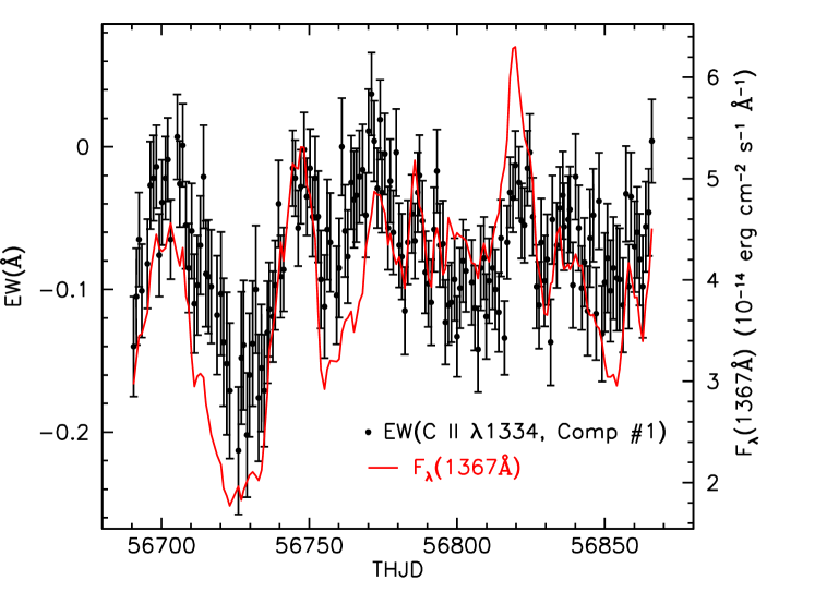
Figure 18: UV continuum light curve at 1367 Å (red line) overlaid on the variations in equivalent width for the absorption in C II $\lambda 1334$ (black points) associated with the intrinsic narrow absorption component #1 in NGC 5548.

This classic ionization response describes the light curves of the low-ionization transitions visible in Component #1. However, this idealized behavior only holds true for approximately the first third of the campaign. At later times, the absorption lines do not follow the continuum so closely, during either the ionization or recombination phases. The correlation plot comparing EW(C II) to the UV continuum flux $\rm F_{\lambda}(1367\mbox{\AA})$ in Figure 19 shows a good linear correlation (linear correlation coefficient $r=0.82$) for the first 75 days of the campaign, or THJD$<$56766, but much more scatter at later times ($r=0.39$).

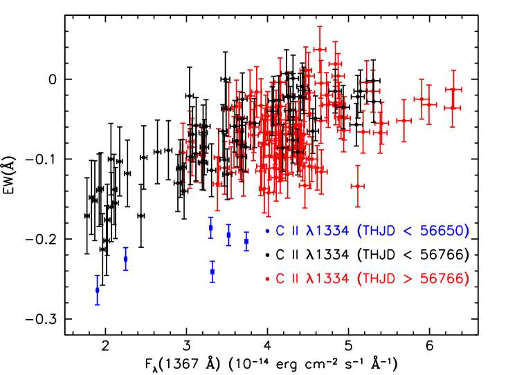
Figure 19: Correlation of the equivalent width of the absorption line C II $\lambda 1334$ associated with the intrinsic narrow absorption component #1 in NGC 5548 with the UV continuum flux at 1367 Å. Blue points are for the six observations of the XMM-Newton campaign, all prior to THJD=56650; black points are for dates in the STORM campaign earlier than THJD=56766; red points are for later times.

A partial explanation for the inconsistent correlation of the absorption line strength with the observed UV continuum is that the observed continuum is only one determinant of the actual ionizing flux beyond the Lyman limit. Historically, the extreme ultraviolet (EUV) continuum varies with greater amplitude than the FUV (Marshall et al. 1997). We also know that the soft X-ray continuum is obscured by optically thick gas that only partially covers the continuum source (Kaastra et al. 2014). This opaque partial coverage also shadows the ionizing ultraviolet, as shown by the photoionization analysis of the UV absorption lines (Arav et al. 2015). The obscuration is also variable, with the variability predominantly explained by variations in the covering fraction (Di Gesu et al. 2015; Cappi et al. 2016; Mehdipour et al. 2016b). If the covering fraction of the obscurer is varying, then one would expect variations in the ionizing flux that are independent of the strength of the observed UV continuum. To test this hypothesis, we did a joint correlation analysis of the variations in EW(C II) with the UV continuum and the hardness ratio as measured with Swift. The hardness ratio is defined as $\rm HR=(HX-SX)/(HX+SX)$, where SX is the soft X-ray count rate in the 0.3–0.8 keV band, and HX is the count rate in the hard X-ray band, 0.8–10.0 keV (Edelson et al. 2015). The hardness ratio is almost a direct measure of the covering fraction of the obscurer (Mehdipour et al. 2016b). A linear fit of the EW(C II) to the UV continuum flux, $F_{\lambda}(1367\mbox{\AA})$ yields the red line shown in Figure 20, with $\chi^{2}$ = 224.2 for 171 points and two degrees of freedom. This is a good correlation, but the fit is not a statistically acceptable predictor of the strength of the EW(C II). If we include the hardness ratio HR as an additional independent variable, the goodness of fit improves dramatically to $\chi^{2}$ = 156.1, which is statistically acceptable. This strongly bolsters the interpretation that the ionizing continuum for C II is determined both by the observed intensity of the UV continuum as well as the fraction of the ionizing continuum that is covered by the X-ray obscurer.

The bottom panel of Figure 20 shows how including HR as a predictor of the EW(C II) improves the fit. The simple red line is the prediction based solely on the UV continuum flux. The observed equivalent widths have a large scatter about this line, as seen in the black points. When the hardness ratio for each observation is taken into account, the predicted equivalent widths then vary from the simple linear fit in a manner consistent with variations in the covering fraction. For a given UV flux, high hardness ratios, indicative of high covering fractions, mean more of the ionizing continuum is obscured, so predicted equivalents widths are greater in magnitude (more negative). For low hardness ratios, covering fractions are lower, more ionizing flux leaks past the obscurer, and equivalent widths decrease in magnitude as more C II is ionized.

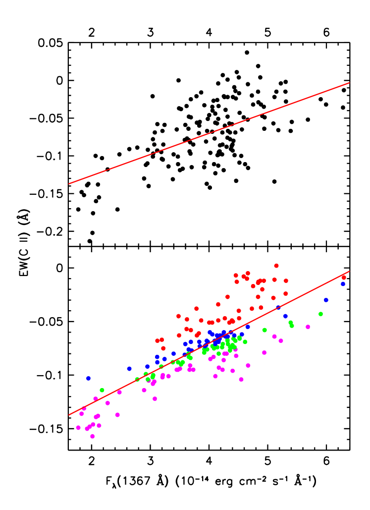
Figure 20: Fits to the correlation of the equivalent width of the absorption line C II $\lambda 1334$ associated with the intrinsic narrow absorption component #1 in NGC 5548 with the UV continuum flux at 1367 Å. The top panel shows EW(C II) (black points) for the entire STORM campaign. The solid red line shows the best-fit linear correlation of EW(C II) with the UV continuum flux, $F_{\lambda}(1367\mbox{\AA})$. (Bottom Panel) Colored points show predicted equivalent widths at a given UV flux for a joint correlation with the Swift hardness ratio, HR. Red points have HR$<$0.768, blue points have 0.768$\leq$HR$<$0.81, green points have 0.81$\leq$HR$<$0.845, and magenta points have HR$\geq$0.845.

An alternative possibility is that the shape of the ionizing continuum is varying, and that the soft X-ray flux might be a good measure of this when combined with the UV continuum flux. We therefore tested a joint correlation of the EW(C II) with the UV continuum flux and the soft X-ray count rate, SX. This also gives an improved fit, $\chi^{2}$ = 180.7, which is statistically acceptable, but not as good as the fit using HR. The improvement can readily be explained as a consequence of SX being determined partially by intrinsic flux variations, but mostly by variations in the covering fraction of the obscurer, as argued by Mehdipour et al. (2016b).

The lack of a direct, exclusive correlation with the observed UV continuum flux is even more striking for all the high-ionization absorption lines, Si IV, C IV and N V. Figure 21 illustrates these effects in the blue component of C IV $\lambda$1548 associated with the absorbing gas in Component #1. This transition has the highest blue-shift of any narrow intrinsic absorption feature for C IV, and therefore it is not blended with any other components. In Figure 21 one can see that it tracks the UV continuum variations very closely up to THJD=56766, both during increases in flux and during decreases in flux. For the first 75 days of the STORM campaign, before the BLR holiday, C IV has a linear correlation coefficient of $r=0.86$. For the remainder of the campaign, however, the correlation drops significantly, with $r=0.06$. In contrast to C II, C IV does not show any recombination delay when continuum flux levels fall, even during the first 75 days of the campaign; the absorption increases in strength almost immediately when the flux levels rise (for THJD$<$56766). The other high-ionization ions, Si IV and N V, also show this instantaneous response. At later times, however, C IV becomes almost completely decorrelated. The correlation plot comparing the EW(C IV) to the UV continuum flux $\rm F_{\lambda}(1367\mbox{\AA})$ in Figure 22 shows a tight correlation with the UV continuum during the first 75 days, just like for C II, but a large degree of scatter at later times. During the period of the BLR holiday, after THJD=56776, there is no coherent correlation between EW(C IV) and the UV continuum flux. The particularly discordant points in the upper right corner of Figure 22 correspond to the FUV continuum flux peak near the end of the holiday period at THJD=56820.

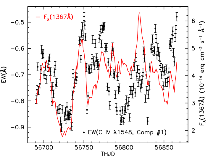
Figure 21: UV continuum light curve at 1367 Å (red line) overlaid on the variations in equivalent width for the absorption in C IV $\lambda 1548$ (black points) associated with the intrinsic narrow absorption component #1 in NGC 5548.

As for C II, we investigated whether other variables might also have a strong correlation with the ionizing flux that is controlling the population of C IV ions. In Figure 23 we compare EW(C IV) to the soft X-ray flux as measured by Swift (Edelson et al. 2015). Although not perfect, the correlation improves significantly, suggesting that the soft X-ray flux plays a more dominant role in controlling the C IV ionic population than the FUV continuum.

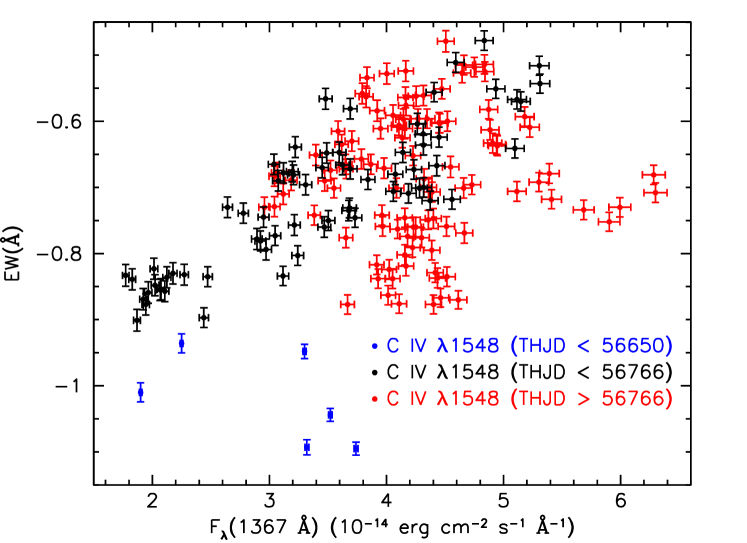
Figure 22: Correlation of the equivalent width of the absorption line C IV $\lambda 1548$ associated with the intrinsic narrow absorption component #1 in NGC 5548 with the UV continuum flux at 1367 Å. Blue points are for the six observations of the XMM-Newton campaign, all prior to THJD=56650; black points are for dates in the STORM campaign earlier than THJD=56766; red points are for later times.

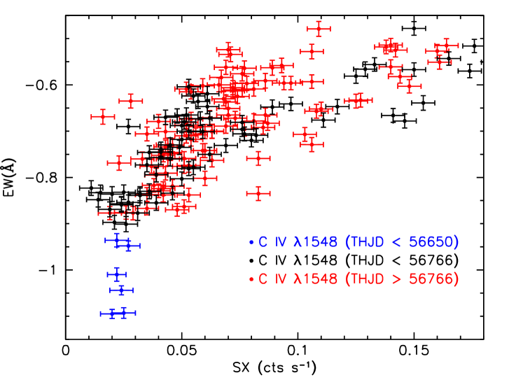
Figure 23: Correlation of the equivalent width of the absorption line C IV $\lambda 1548$ associated with the intrinsic narrow absorption component #1 in NGC 5548 with the Swift soft X-ray (SX) count rate. Blue points are for the six observations of the XMM-Newton campaign, all prior to THJD=56650; black points are for dates in the STORM campaign earlier than THJD=56766; red points are for later times.

Again, we investigated whether a multivariate correlation would be better than either continuum measure on its own. First, as expected, a simple linear fit of EW(C IV) vs.  $F_{\lambda}(1367\mbox{\AA})$ is statistically unacceptable with $\chi^{2}$=6271 for 171 points and 2 free parameters. We then included the hardness ratio, HR, in the correlation, leading to a dramatic improvement, but the fit is still poor with $\chi^{2}$=4314. Finally, in contrast to C II, using the soft X-ray flux in tandem with $F_{\lambda}(1367\mbox{\AA})$ gives the best result, $\chi^{2}$=3608. This is still statistically unacceptable, but it does show the stronger influence that the soft X-ray continuum is having on the C IV ionization than the far-UV continuum. As a final trial, assuming that the hardness ratio, HR, might serve as an an additional measure of the covering fraction of the obscurer, we carried out a trivariate analysis using SX, $F_{\lambda}(1367\mbox{\AA})$, and HR. This provided no additional improvement in $\chi^{2}$, with $\Delta\chi^{2}<1$. Figure 24 shows the correlation of the EW(C IV) with $F_{\lambda}(1367\mbox{\AA})$, and how including SX as an additional independent variable improves the fit. Much of the scatter about the linear fit is explained by variations in the soft X-ray flux. The low equivalent width points in the upper right corner of the top panel of Figure 24 coincide with some of the lowest soft X-ray fluxes observed as shown in the bimodal fit presented in the bottom panel. The fact that it is the soft X-ray flux directly rather than just a covering factor effect (as for C II) may be telling us that the extreme ultraviolet (EUV) and soft X-ray continuum shape is also varying, since it is this portion of the continuum that is responsible for ionizing C IV. This is not the whole story, however. As shown in Figure 24, there is a large set of points (shown in green) where variations in EW(C IV) are not explained either by UV or soft X-ray continuum variations. These green points encompass times from THJD=56776 to 56827. This evidence, plus the complete decoupling from the continuum variations in the light curve after THJD$\sim$56750, appears to be related to the BLR holiday (Goad et al. 2016), which sets in at the same time. The green points in Figure 24 lie in the deepest portion of the BLR holiday. In Paper VII (Mathur et al. 2017) we speculated that the BLR holiday was related to changes in the EUV/soft X-ray continuum shape, and that these changes in the higher-energy range of the spectral energy distribution (SED) were not reflected in the visible FUV continuum. The responses of the high-ionization intrinsic absorption lines enable us to directly measure these changes in the SED.

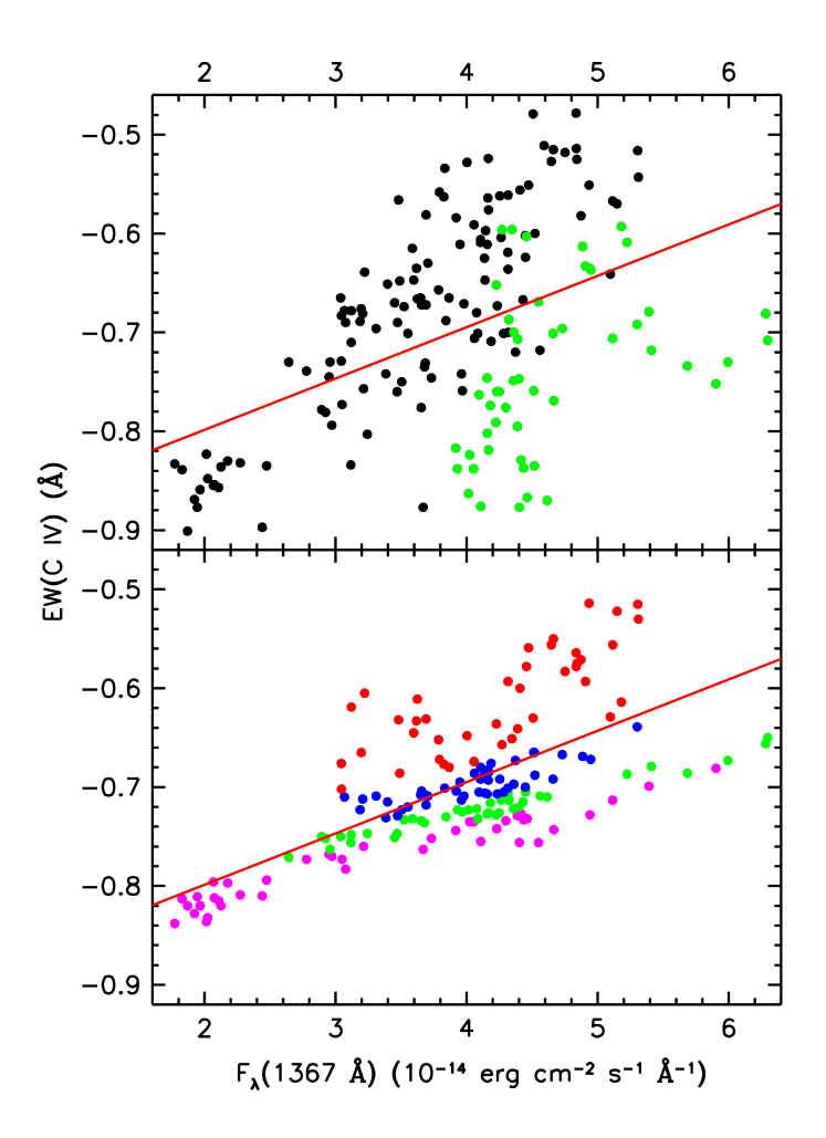
Figure 24: Fits to the correlation of the equivalent width of the absorption line C IV $\lambda 1548$ associated with the intrinsic narrow absorption component #1 in NGC 5548 with the UV continuum flux at 1367 Å. (Top Panel) Black and green points are for the entire STORM campaign. Green points show values for EW(C IV) during the depths of the BLR holiday, for times 56776$<$THJD$<$56827. The solid red line shows the best-fit linear correlation of EW(C IV) with the UV continuum flux, $F_{\lambda}(1367\mbox{\AA})$. (Bottom Panel) Colored points show predicted equivalent widths at a given UV flux for a joint correlation with the Swift soft X-ray flux from 0.3–0.8 keV, SX. Red points have SX$>$0.085, blue points have 0.085$\geq$SX$>$0.058, green points have 0.058$\geq$SX$<$0.043, and magenta points have SX$<$0.043.

While the responses of the broad emission lines also give insight into the behavior of the continuum, their large-scale spatial distribution and differing views of the continuum source complicate such an analysis. Since the narrow intrinsic absorption lines in NGC 5548 are directly along our line of sight, they are exposed to the same continuum that we see. This allows us to take advantage of their unique point of view and to obtain a direct measure of the continuum strength at a variety of energies. To a good first approximation, the continuum flux at an ion’s ionization potential is the ionizing flux driving the population of that ion. To use the strength of the absorption lines as a measure of this flux, however, we must be certain that the absorption line variations are reflecting changes in column density in response to changes in the ionizing flux rather than being caused by either variations in covering factor, transverse motion, or both.

The best evidence in favor of a dominant photoionization response is the good correlation we see between the strength of the individual absorption lines and either the FUV continuum (for low-ionization lines like C II), or the soft X-ray flux (for high-ionization lines like C IV). Our biggest concern is for C IV because it was heavily saturated during the XMM-Newton campaign. The photoionization models of Arav et al. (2015) show that it has an optical depth of 200 during the observations in 2014. Figure 25 shows that the bottom of the absorption trough in C IV $\lambda 1548$ Component #1 remained relatively constant in 2014, in agreement with heavy saturation. Likewise, Figure 23 shows that during the XMM-Newton campaign, the strength of the absorption in C IV $\lambda 1548$ Component #1 is independent of the soft X-ray flux, and much stronger than during the AGN STORM campaign. In contrast, Figure 23 shows a strong correlation with the soft X-ray flux during the AGN STORM campaign, indicative of a photoionization response. In Figure 26, we show that the absorption line profiles change as expected if the column density in C IV Component #1 was varying in response to changes in the ionizing flux.

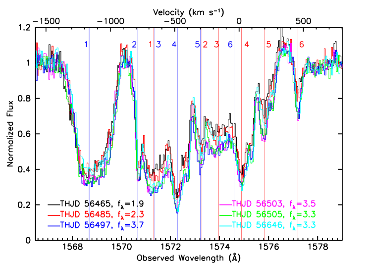
Figure 25: Illustration of variability in the narrow absorption components of C IV in NGC 5548 during the XMM-Newton campaign (Kaastra et al. 2014). Normalized relative fluxes are plotted as a function of velocity relative to the systemic redshift of $z=0.017175$ for C IV $\lambda 1548$, The colored curves are the spectra for the observation dates given in the key along with the observed flux at 1367 Å in units of $10^{-14}~{}\rm erg~{}cm^{-2}~{}s^{-1}~{}\mbox{\AA}^{-1}$. Thin vertical blue lines indicate the velocities of the blue components of the doublets for the six intrinsic absorbers. Vertical red lines show the locations of the corresponding red components. Component #1 shows little variability during the campaign, indicating high saturation.

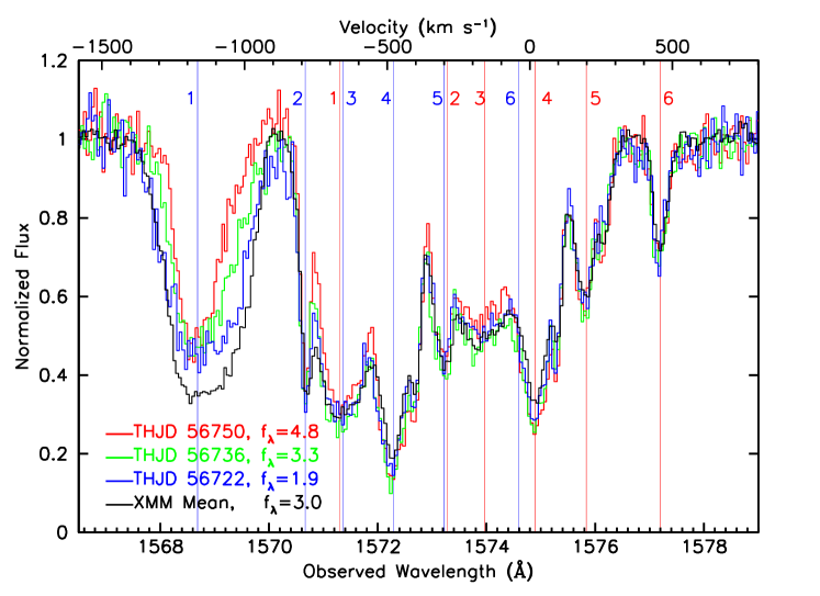
Figure 26: Illustration of variability in the narrow absorption components of C IV in NGC 5548 campaign during the early part of the AGN STORM campaign when the strength of C IV absorption in Component #1 was highly correlated with the FUV continuum flux. Normalized relative fluxes are plotted as a function of velocity relative to the systemic redshift of $z=0.017175$ for C IV $\lambda 1548$, The colored curves are the spectra for the observation dates given in the key along with the observed flux at 1367 Å in units of $10^{-14}~{}\rm erg~{}cm^{-2}~{}s^{-1}~{}\mbox{\AA}^{-1}$. The illustrated spectra show high (red), low (blue), and mean (green) flux levels in comparison to the mean spectrum from the XMM-Newton campaign (black). Thin vertical blue lines indicate the velocities of the blue components of the doublets for the six intrinsic absorbers. Vertical red lines show the locations of the corresponding red components. During AGN STORM, the absorption profile in Component #1 varies as expected for gas showing an ionization response.

Assuming that the absorption lines in Component #1 are indeed tracing a response to change in the ionizing flux, we can use this behavior as a diagnostic of the ionizing continuum. For the first 75 days of the campaign (dates prior to THJD=56766) both the absorption lines and the emission lines show a good correlation in their variations with the FUV continuum flux at 1367 Å. We use this proportionality to derive a linear relationship between a line’s EW and the continuum flux of

$$\rm EW=a_{0}+a_{1}\times F_{\lambda}(1367).$$ (19)

During this early part of the campaign, when everything correlates well, we assume that the continuum shape is that shown in Figure 4 of Mehdipour et al. (2015). We designate points lying on this fiducial SED as $\rm F_{0}(\lambda)$, where $\lambda$ may be either the observed wavelength 1367 Å, or the wavelength at the ionization potential of the relevant ion, $\lambda_{\rm IP}$. We can then use variations in the EW of a given line to measure changes in the flux at the ionization potential relative to this fiducial SED shape of

$$\rm\frac{F(\lambda_{IP})}{F_{0}(\lambda_{IP})}=\frac{(EW-a_{0})/a_{1}}{F_{0}(1367)}.$$ (20)

Following this methodology, we derive relative ionizing continuum light curves for each absorption line representative of the time-varying relative fluxes at their ionization potentials. Figure 27 shows these relative light curves for the blue components of the Si IV, C IV and N V doublets of the intrinsic absorption line for Component #1 in NGC 5548. The figure also compares these relative light curves to the deficiency in the broad C IV emission line flux during the BLR holiday (Goad et al. 2016), defined as the percentage diminution in the C IV emission line flux during the holiday compared to the expected flux based on the correlation of C IV emission line flux with continuum flux observed during the first 75 days of the AGN STORM campaign. Note that the relative decrease in broad C IV emission line flux occurs during the same time interval (56776$<$THJD$<$56827) as the inferred decrease in EUV continuum flux at the ionization potentials of Si IV (45.1 eV), C IV (64.5 eV) and N V (97.9 eV) deduced from the behavior of the intrinsic absorption line. All three inferred continua show significant correlations with the deficit in the C IV emission. However, there is a delay between the C IV deficit and the inferred continua. Using ICCF, we find delays and peak correlation coefficients of $11.6\pm 1$ days and $r=0.66$ for Si IV, $10.5\pm 1$ days and $r=0.70$ for C IV, and $12.3\pm 1$ days and $r=0.64$ for N V. These delays are actually with respect to the FUV continuum at 1158 Å, since Goad et al. (2016) shifted the C IV light curve by $-5$ days to align it with the continuum variations, so the inferred EUV continua variations are delayed by 5–7 days relative to the C IV deficit. These delays are puzzling since one might expect the C IV deficit to lag the continuum deficits rather than vice versa if they were the direct cause of the BLR holiday. Dehghanian et al. (2019) investigate the complex responses of the intrinsic narrow absorption lines to changes in the ionizing continuum and the intervening obscurer in greater detail although they also do not explain this puzzling behavior.

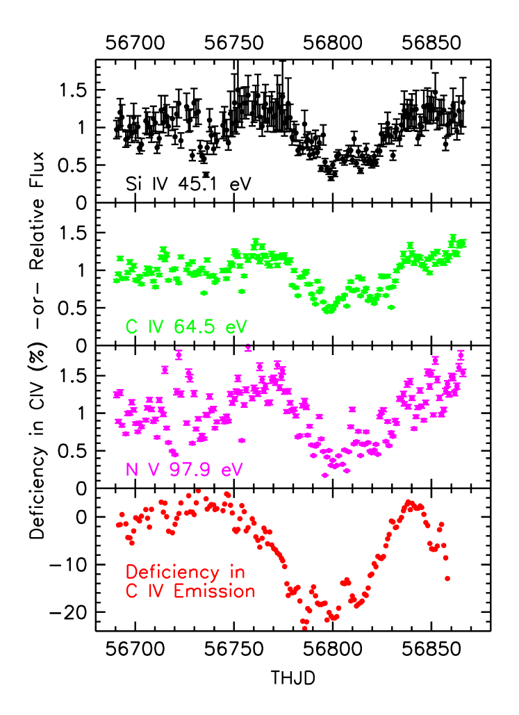
Figure 27: Relative EUV continuum fluxes at the ionization potentials of Si IV (45.1 eV, black points), C IV (64.5 eV, green points) and N V (97.9 eV, magenta points) as deduced from variations in the equivalent width of the absorption lines Si IV $\lambda 1393$, C IV $\lambda 1548$ and N V $\lambda$1238 associated with the intrinsic narrow absorption component #1 in NGC 5548. Red points show the percentage deficiency in the flux of C IV broad emission during the BLR holiday (Goad et al. 2016).

4.4 Variability of the Broad Absorption Features

As discussed in §5.2, the broad absorption features that appear as extensive blue-shifted troughs on all the resonant UV lines in the spectrum of NGC 5548 are the UV counterparts to the soft X-ray obscurer discovered by Kaastra et al. (2014). These broad UV absorption features also vary with time. In fact, in the observations from that campaign, there was a significant anticorrelation between the strength of the absorption troughs and the soft X-ray flux as measured by Swift (linear correlation coefficient $r=-0.37$). As the soft X-ray intensity increased, the broad UV absorption strength decreased. This is not due to a photoionization response, however. The broad UV absorption lines are saturated, and so their strength is also governed more by the covering factor than by the ionization state or column density of the absorbing gas.

The more extensive monitoring of the time variability of the broad absorption features enabled by the STORM campaign reveals an even more complex picture. As shown in Figure 28, the anticorrelation of the EW of the broad absorption is not as clean as it was in the six points available from the XMM-Newton campaign.

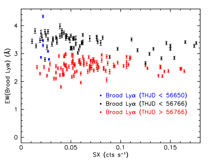
Figure 28: Correlation of the absolute value of the equivalent width of the broad absorption in Ly$\alpha$ in NGC 5548 with the soft X-ray flux from Swift. Blue points are for the six observations of the XMM-Newton campaign, all prior to THJD=56650; black points are for dates in the STORM campaign earlier than THJD=56766; red points are for later times.

While there is a rough anticorrelation ($r=-0.41$) early in the campaign (THJD$<$56766), as with the behavior of the narrow absorption lines, the correlation disappears after THJD=56766 ($r=+0.02$), approximately the time of the onset of the BLR holiday (Goad et al. 2016). Figure 29 shows this even more dramatically. Light curves for the EWs of the broad absorption features are eerily similar to the time variation of the anomalous deficit in the response of the flux of the broad emission lines. The connection between these two behaviors is puzzling. On the one hand, the lack of response in the BLR during the holiday appears to be due to a change in the SED, in which the soft X-ray excess decouples from the visible UV continuum. A decrease in the BLR flux during the holiday implies a decrease in the ionizing UV driving the line emission. On the other hand, a decrease in the broad absorption line EW implies a decrease in the covering factor of the obscurer, because these broad troughs appear to be saturated (§4.2) and we see no dramatic changes in their velocity widths.. This is also seen in the Swift monitoring of NGC 5548 (Mehdipour et al. 2016b), and it implies that more of the EUV and soft X-ray flux is being transmitted past the obscurer. Plus, since the BLR response represents a global view of the continuum source, and our view of the obscurer is restricted purely to our line of sight, this suggests that our view of the obscurer may not be a special geometrical arrangement, such as a single cloud crossing our line of sight, but rather a more axisymmetric arrangement affecting all sightlines that illuminate the BLR. Dehghanian et al. (2019) present further photoionization analysis of both the narrow and the broad absorbers that support this interpretation.

An approximate axisymmetric arrangement for the obscurer is even more natural when one considers the timescales covered by our observations. From the beginning of the XMM-Newton campaign in June 2013 to the end of the reverberation mapping campaign in July 2014, the elapsed time was 415 days. For a black-hole mass of $5.2\times 10^{7}~{}\rm M_{\sun}$ (Bentz & Katz 2015), clouds at a radius of 1 light day, at the innermost edge of the BLR. would have an orbital timescale of 115 days. Thus the obscurer and the innermost part of the BLR could have completed more than one full revolution over the course of our observing programs.

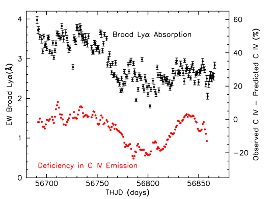
Figure 29: Light curve of the variations in the absolute value of the equivalent width of broad Ly$\alpha$ absorption in NGC 5548 (black points) compared to the percentage deficiency in the flux of C IV broad emission (red points) during the BLR holiday (Goad et al. 2016).

5 Discussion

Modeling the UV spectra of NGC 5548 from the STORM campaign accomplished our primary goal of obtaining clean, absorption-corrected, deblended emission-line profiles of all the principle UV emission lines. We are also able to separate the non-varying contributions of the narrow-line and intermediate line emission to the Ly$\alpha$ and C IV profiles and produce uniform velocity-binned lag measurements across the full profiles of Ly$\alpha$ and C IV. These “clean” line profiles are a key element for future detailed modeling of the BLR to produce two-dimensional velocity delay maps using both MEMEcho (Horne et al. 2019) and forward-modeling techniques (Pancoast et al. 2019). However, simple characteristics of the emission-line profiles and the one-dimensional velocity delay profiles enable us to make some key inferences.

The Ly$\alpha$ velocity delay profile shows a distinctive “M” shape, with short lags at high velocity, peak lags of $\sim 6-8$ days at moderate velocities ($\pm 2500~{}\rm km~{}s^{-1}$), and a local minimum near zero velocity. As we discuss in more detail later, this is very different from the centrally peaked H$\beta$ profile observed in 2007 by Denney et al. (2009). The C IV velocity delay profile is similar to Ly$\alpha$, but it shows only “shoulders” rather than a central dip. This behavior was seen in the original raw data (De Rosa et al. 2015), but we now have a clean, uniform picture across both profiles. This morphology is very similar to that seen in H$\beta$ during the ground-based portion of the STORM campaign (Pei et al. 2017) as well as during the 2015 campaign by Lu et al. (2016) and Xiao et al. (2018).

The short lags at high velocity and longer lags at low velocity are a natural expectation for Keplerian profiles in a disk (Welsh & Horne 1991; Horne et al. 2004). In a simple disk geometry where the line-emitting portion of the disk is truncated at both an inner and an outer radius, the lag profile across the emission line extends from short lags at high velocities, corresponding to the inner radius of the disk, and rises to peaks at lower velocities, corresponding to the outer radius of the disk (Welsh & Horne 1991). In the region near zero velocity, the near-zero lags from the near side of the disk produce a central dip. The sharp peaks of the lag profile produced by a thin disk in the models of Welsh & Horne (1991) is a direct consequence of their disk model having a monotonic, powerlaw emissivity and sharp edges. This leads to a “cuspy” shape for the transfer function, $\Psi(\tau)$. The sharp peaks can be broadened into smoother bumps if the line-emitting portions of the disk do not have abrupt edges, and if the disk is thickened, as in Pancoast et al. (2014), for example. In the case of NGC 5548, the transfer function $\Psi(\tau)$ recovered from the data is smooth and bell-shaped (Horne et al. 2019), which would result in smooth, round peaks in the lag profile.

Notably, the lag profile for C IV for the full campaign shows an upturn to longer lags at high positive velocities ($>10,000~{}\rm~{}km~{}s^{-1}$). This feature was not evident in the original raw data, but may now appear when the contamination of the red wing of C IV by the shorter lag of He II may have been biasing the result to lower values. Longer lags at high positive velocities are indicative of outflowing gas since redshifted, outflowing gas is on the far side of the illuminating source relative to the observer. See the models of Welsh & Horne (1991) for examples. These long lags at high positive velocities are absent when we restrict the data to the first 75 days of the campaign before the BLR holiday.

The C IV lag profile shows additional changes in structure for different time intervals during the campaign, as discussed in §4.1. The biggest change is the apparent change from a local minimum in the lag on the red side of the red emission bump in the pre-holiday period to a local maximum on the blue side of the bump during the holiday period. These changes are in contrast to smoother, more uniform changes for Ly$\alpha$, which mostly track the evolution to longer lags of the mean profile at all velocities across the profile. Although we cannot unambiguously assign physical explanations to one-dimensional emission-line and lag profiles, the difference in behavior between C IV and Ly$\alpha$ may reflect the differences in radiative transfer through the BLR for these two emission lines. Both lines are generally considered to be optically thick, with preferential emission originating from the illuminated side of the BLR gas (Kwan & Krolik 1979, 1981; Ferland et al. 1992), but the smoother evolution of the lag profile during the course of the campaign may suggest that Ly$\alpha$ emission is less orientation dependent than that of C IV.

The lag profiles across the emission lines in NGC 5548 have also evolved on longer timescales over the past decade. In the 2007 observations of the H$\beta$ profile by Denney et al. (2009), the lag profile is centrally peaked with no dip, and it extends to velocities of only $\pm 6000~{}\rm km~{}s^{-1}$. For a black hole mass of $\rm M_{BH}=5.2\times 10^{7}~{}M_{\odot}$ (Bentz & Katz 2015) and an inclination of $i=32^{\circ}$ (Pancoast et al. 2014), this corresponds to Keplerian velocities at an inner disk radius of 2.3 light days. The innermost bins span a range of $\pm 1000~{}\rm km~{}s^{-1}$/sin $i$, which correspond to Keplerian velocities at an outer disk radius of $\sim 80$ light days.

The AGN12 campaign (De Rosa et al. 2018) showed that by 2012 NGC 5548 had developed a double peaked, “M”-shaped lag profile. By the time of the STORM campaign in 2014, this shape was well developed in both H$\beta$ and in Ly$\alpha$. For the STORM data, profiles reaching velocities of $\pm 10\,000~{}\rm km~{}s^{-1}$ imply an inner disk radius of $\sim 0.8$ light day. The double peaks at $\pm 2500~{}\rm km~{}s^{-1}$ lead to an outer disk radius of 13 light days.

These changes in the implied overall structure of the BLR may explain the departure of its measured size from the previously well established BLR size/luminosity relation (see Fig. 13 of Pei et al. 2017) as the luminosity of NGC 5548 has evolved in time over the past two decades. Figure 30 compares the evolution in the optical luminosity ($\lambda\rm L_{5100}$) of NGC 5548 to the size of the BLR as measured by the reverberation lag of the H$\beta$ emission line. During the 2007 campaign of Denney et al. (2009), NGC 5548 was near a minimum in its luminosity. The integrated H$\beta$ lag was 5 days, and it fit well on the BLR size/luminosity relation. In 2012, NGC 5548 increased to normal brightness levels, but the overall H$\beta$ lag remained low at 4 days (De Rosa et al. 2018). One must be careful in assessing the absolute values of these changes in size, however. Goad & Korista (2014) note that emission line lags can be biased low by factors of 2–3 for short continuum variability timescales (as we observed in the STORM campaign), and for campaigns of short duration (as were those in the 2000s). During the lengthy STORM campaign in 2014, NGC 5548 remained bright, yet the H$\beta$ lag remained small, at 4 days, factors of 5–6 smaller than historical values in the 1990s. Notably, these changes coincide with the appearance of the X-ray obscurer in February 2012, as shown in data from Swift monitoring (Mehdipour et al. 2016b).

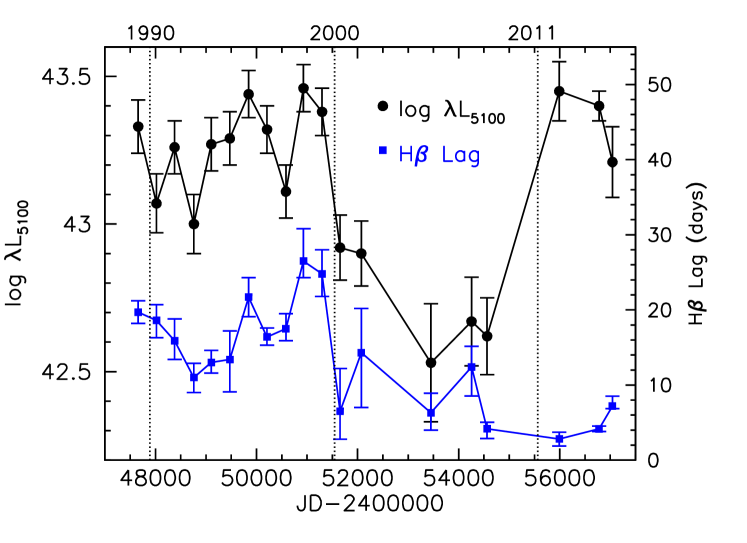
Figure 30: Time series showing the history of the optical luminosity of NGC 5548 ($\lambda\rm L_{5100}$, black points) and the reverberation lag size for the H$\beta$ emission line (blue points). Vertical dotted lines show the dates 1990 January 1, 2000 January 1, and 2011 January 1. Data prior to 2011 are from Kilerci Eser et al. (2015), which are taken from these original sources: Peterson et al. (2002), Bentz et al. (2007), Bentz et al. (2009), Denney et al. (2009), and Peterson (1993). Data in 2012 are from De Rosa et al. (2018). Data in 2014 are from the STORM campaign (Pei et al. 2017). Data in 2015 are from Lu et al. (2016).

Similar behavior has been seen in NGC 3783. This Seyfert 1 also exhibited an obscuration event in 2016 with heavy, soft X-ray and broad UV absorption (Mehdipour et al. 2017). When the obscuration appeared, NGC 3783 was at a luminosity peak following a low-luminosity state from 2011 through 2014 (Kaastra et al. 2018). Despite the high luminosity, its broad lines were significantly diminished in flux, with moderate velocity regions ($\sim 2800~{}\rm km~{}s^{-1}$) of the profile apparently gone (Kriss et al. 2019). Kriss et al. (2019) suggest that the changes in the structure of the BLR and the appearance of the obscuring outflow are related. In the context of disk-driven wind models (Murray & Chiang 1997; Proga et al. 2000; Proga & Kallman 2004; Proga & Waters 2015; Waters & Proga 2016; Czerny et al. 2017; Baskin & Laor 2018), the transition from a normal BLR configuration to an extended low state requires several years for the BLR to dynamically adjust to the reduced radiation pressure from the accretion disk. The BLR at large radii collapses back toward the disk plane, and the peak in the BLR emissivity shifts to smaller radii. When the continuum brightens, the excess material in the inner regions may be blown away as a radiatively driven wind, observable as the obscurer. The BLR reinflates, but this requires years, governed by the free-fall timescale for the disk wind, which is 3.4 years at 10 light days in NGC 3783 for a black hole mass of $\rm M_{BH}=2.3\times 10^{7}~{}M_{\odot}$ (Bentz & Katz 2015).

Timescales in NGC 5548 are similar, but shorter, given its slightly higher black hole mass. At 10 light days in NGC 5548, Keplerian velocities are $\sim 5200~{}\rm km~{}s^{-1}$, and the free-fall time, defined as

$$\rm t_{ff}=\left(\frac{2R^{3}}{GM_{BH}}\right)^{1/2},$$ (21)

is 2.3 years. The shrunken size of the BLR during the STORM campaign is also reflected in the lack of stratification in the ionization structure that was evident in past campaigns (Clavel et al. 1991; Korista et al. 1995). Except for He II, all the other broad emission lines have indistinguishable lags. After the STORM campaign, in 2015 NGC 5548 appears to be reverting back to the normal size/luminosity relation. Lu et al. (2016) observed an increase in the H$\beta$ lag to 7 days. They suggest that this evolution in size was evidence for radiation pressure affecting the size of the BLR, with a time delay likely due to the dynamical timescale of the BLR, similar to our arguments above.

Although our modeling of the UV spectra from the NGC 5548 STORM campaign have enabled us to understand the dynamics of the BLR better, and its potential links to the appearance of X-ray and UV obscuration, we must still work out the details of what produces the short timescale variations in the obscuring gas, and how that affects the BLR emission. These processes will be subjects of future papers.

6 Summary

We have modeled the HST UV spectra of NGC 5548 obtained during the 2014 Space Telescope and Optical Reverberation Mapping (STORM) campaign. The model uses 97 emission and absorption components to construct an emission model for all 171 spectra of NGC 5548 obtained during the campaign. The model permits us to separate the broad absorption associated with the soft X-ray obscuration discovered by Kaastra et al. (2014), and to correct for narrow absorption produced by the intrinsic UV absorption lines of NGC 5548 as well as intervening interstellar features. Using the model, we are able to produce absorption-corrected, deblended emission-line profiles, velocity-binned light curves for Ly$\alpha$ and C IV, and light curves for all narrow and broad absorption components. The modeled emission-line profiles eliminate the non-varying flux of the narrow-line and intermediate-line components of Ly$\alpha$ and C IV, separate the contributions of N V and He II to their profiles, and give a clear view of the emission-line time delay across the full line profile. The principle results of our study are:

1. The time lags of 2–8 days for the integrated emission lines are comparable to, or slightly shorter than those in De Rosa et al. (2015), primarily due to the elimination of the non-varying narrow-line and intermediate-line components (§4.1).

2. The velocity-binned lag profiles have a distinct “M” shape in Ly$\alpha$, and less-prominent local maxima above a central minimum in C IV (§4.1). The local minima in the lag profiles are near zero velocity, and the local peaks (Ly$\alpha$) or shoulders (C IV) are at $\pm 2500~{}\rm km~{}s^{-1}$ (§4.1). This morphology is indicative of Keplerian motion in a disk-like configuration.

3. The narrow absorption lines vary in strength in response to changes in the continuum intensity (§4.3). The lowest ionization absorption lines (Ly$\alpha$, C II, and Si II) correlate with the continuum through the course of the whole campaign. Their variations show a delayed and smoothed response to continuum variations consistent with recombination of gas with densities of $\rm log~{}n_{e}~{}cm^{-3}\sim 5$, similar to the density measured by Arav et al. (2015) using density-sensitive absorption lines of C III* and Si III*, and similar to the density of the NLR inferred by Kraemer et al. (1998) and Peterson et al. (2013).

4. High-ionization intrinsic narrow absorption lines (Si IV, C IV, and N V) correlate well with the continuum during the first 75 days of the campaign (§4.3). Thereafter, they decorrelate, showing signs of the same “holiday” exhibited by the BLR (Goad et al. 2016). During the holiday period, their strengths correlate most closely with the soft X-ray flux as measured by Swift, which suggests that the soft X-ray flux is more closely related to the ionizing extreme ultraviolet than the FUV continuum. Using the response of these high-ionization absorption lines, we are able to reconstruct the relative flux of the spectral energy distribution in the extreme ultraviolet. We show that it is diminished in flux relative to the FUV continuum during the period of the holiday.

5. The broad absorption lines associated with the X-ray obscurer also vary during the course of the campaign (§4.4). Early in the campaign, they show a rough anticorrelation with the soft X-ray flux, as seen by Kaastra et al. (2014). However, during the holiday period they decrease in strength, with behavior mimicking the deficiencies in the flux of the broad emission lines. This behavior is not understood.

6. The departure of NGC 5548’s BLR from the radius/luminosity relationship of Peterson et al. (2002) during the AGN12 campaign in 2012 (De Rosa et al. 2018) coincides with the appearance of the X-ray obscurer at about the same time (Mehdipour et al. 2016b). We suggest the two events are related, and that the obscurer is a manifestation of a disk wind launched by the brightening of NGC 5548 in 2012 after a prolonged low-luminosity state which had led to the collapse of the BLR (§5).

Modeling the UV spectra of NGC 5548 from the STORM campaign has yielded crucial insights into the behavior of the emission-line and absorption-line gas as well as properties of the ionizing continuum that were not easily seen in the raw data. These new insights may help us to resolve the structure of the BLR and successfully interpret our measures of its two-dimensional reverberation maps.

Table 1: Model Parameters for the Mean Spectrum of NGC 5548

Feature	Component	$\rm\lambda_{vac}$	$\rm\lambda_{obs}$	Flux	FWHM	Asymmetry	Freedom
	Number	(Å)	(Å)		($\rm km~{}s^{-1}$)		Flags
Power Law $\rm F_{\lambda}$(1000)	1	5.978					0
Power Law $\alpha$	1	0.840					0
E(B$-$V)	2	0.017					$-$1
$\rm R_{V}$	2	3.1					$-$1
Galactic Ly$\alpha$	66	1215.67	1215.55	1.45			$-$1
C III*	3	1175.78	1195.01	1.06	861	1.00	0,0,0,$-1$
C III* Broad	95	1175.78	1195.01	3.13	3000	1.00	0,0,0,$-1$
Si III	4	1206.50	1226.39	1.44	861	1.00	0,0,3,$-1$
Ly$\alpha$ Narrow	5	1215.67	1236.55	19.3	255	1.00	0,0,0,$-1$
Ly$\alpha$ Intermediate	6	1215.67	1236.00	67.3	861	1.00	0,0,0,$-1$
Ly$\alpha$ Broad	7	1215.67	1235.14	176.0	3047	1.00	0,0,0,$-1$
Ly$\alpha$ Medium Broad	8	1215.67	1231.59	340.0	8074	1.00	0,0,0,$-1$
Ly$\alpha$ Very Broad	9	1215.67	1237.64	154.0	18347	1.00	0,0,0,$-1$
Ly$\alpha$ Red Bump	21	1215.67	1243.04	1.73	713	1.00	0,0,0,$-1$
N V Narrow	10	1238.82	1259.75	1.22	255	1.00	0,0,5,$-1$
N V Narrow	11	1242.80	1263.80	1.22	255	1.00	10,10,10,$-1$
N V Intermediate	12	1238.82	1259.53	0.62	861	1.00	6,0,6,$-1$
N V Intermediate	13	1242.80	1263.58	0.62	861	1.00	12,12,12,$-1$
N V Broad	14	1238.82	1258.66	23.3	3047	1.00	7,0,7,$-1$
N V Broad	15	1242.80	1262.70	23.3	3047	1.00	14,14,14,$-1$
N V Medium Broad	16	1238.82	1255.04	6.85	8074	1.00	8,0,8,$-1$
N V Medium Broad	17	1242.80	1259.08	6.85	8074	1.00	16,16,16,$-1$
N V Very Broad	18	1240.01	1263.24	40.8	18347	1.00	9,0,9,$-1$
S II	19	1253.81	1273.00	0.09	841	1.00	0,0,0,$-1$
Si II	20	1260.42	1281.00	5.39	3500	1.00	0,0,0,$-1$
O I Narrow	48	1302.17	1323.52	0.10	359	1.00	0,0,0,$-1$
Si II Narrow	49	1304.37	1327.01	0.20	359	1.00	0,0,48,$-1$
Si II+O I Broad	50	1303.27	1329.35	13.1	4659	1.00	0,0,0,$-1$
Unknown	47	$\ldots$	1317.76	1.24	1687	1.00	0,0,0,$-1$
C II Intermediate	94	1334.53	1358.00	0.83	861	1.00	0,0,34,$-1$
C II Broad	51	1334.53	1357.36	2.28	3000	1.00	0,0,$-1$,$-1$
Si IV Narrow	96	1393.76	1416.74	0.41	303	1.00	0,0,0,$-1$
Si IV Narrow	97	1402.77	1425.90	0.20	303	1.00	96,96,96,$-1$
Si IV Intermediate	23	1393.76	1415.97	1.67	842	1.00	0,0,0,$-1$
Si IV Intermediate	24	1402.77	1425.13	0.84	842	1.00	23,23,23,$-1$
Si IV Broad	25	1393.76	1416.74	9.29	4889	1.00	0,0,0,$-1$
Si IV Broad	26	1402.77	1425.90	9.29	4889	1.00	25,25,25,$-1$
Si IV Medium Broad	27	1393.76	1415.28	12.5	8704	1.00	0,0,0,$-1$
Si IV Medium Broad	28	1402.77	1424.43	12.5	8704	1.00	27,27,27,$-1$
Si IV Very Broad	29	1398.26	1409.20	37.1	18148	0.92	0,0,0,$-1$
O IV]	52	1400.00	1425.92	6.00	1858	1.00	0,0,0,$-1$
N IV] Intermediate	39	1486.00	1510.54	3.30	1050	1.00	0,0,0,$-1$
N IV] Broad	22	1486.00	1512.13	1.83	3800	1.00	0,0,$-1$,$-1$
C IV Narrow	30	1548.20	1574.34	7.86	303	1.00	0,0,0,$-1$
C IV Narrow	31	1550.77	1576.96	7.86	303	1.00	32,32,32,$-1$
C IV Intermediate	32	1548.20	1574.32	21.4	861	1.00	0,0,0,$-1$
C IV Intermediate	33	1550.77	1576.93	21.4	861	1.00	34,34,34,$-1$
C IV Broad	34	1548.20	1574.28	62.3	3366	1.00	0,0,0,$-1$
C IV Broad	35	1550.77	1576.90	62.3	3366	1.00	36,36,36,$-1$
C IV Medium Broad	36	1548.20	1569.00	98.5	8345	1.00	0,0,0,$-1$
C IV Medium Broad	37	1550.77	1571.61	98.5	8345	1.00	0,0,0,$-1$
C IV Very Broad	38	1550.48	1577.99	286.0	16367	1.00	0,0,0,$-1$
C IV Blue Bump	93	1550.48	1553.79	7.53	1900	1.00	0,0,0,$-1$
C IV Red Bump	74	1550.48	1603.34	3.95	1708	1.00	0,0,0,$-1$
He II Narrow	40	1640.45	1667.66	1.01	303	1.00	0,0,30,$-1$
He II Intermediate	41	1640.45	1667.40	5.22	861	1.00	0,0,32,$-1$
He II Broad	42	1640.45	1669.07	6.18	3366	1.00	0,0,34,$-1$
He II Medium Broad	43	1640.45	1667.10	41.5	8345	1.00	0,0,36,$-1$
He II Very Broad	67	1640.45	1667.14	4.93	16367	1.00	0,0,38,$-1$
O III] Narrow	92	1660.00	1686.82	0.87	771	1.00	0,47,0,$-1$
O III] Narrow	44	1666.00	1693.74	1.64	555	1.00	0,0,0,$-1$
O III] Broad	45	1663.00	1693.23	13.5	3639	1.00	0,0,0,$-1$
Unknown	68	$\ldots$	1709.64	2.91	3366	1.00	0,0,0,$-1$
N III] Broad	46	1750.00	1781.33	7.56	3801	1.00	0,0,0,$-1$
Fe II	53	$\ldots$	$\ldots$	13.91	1861.0	$\ldots$	$-1$,0,0,$-1$
C III* Broad Absorption	54	1175.78	1194.00	$-$0.01	3796	0.13	0,0,55,55
Ly$\alpha$ Broad Absorption	55	1215.67	1235.00	$-$71.62	3796	0.13	0,0,0,0
N V Broad Absorption	56	1238.82	1258.00	$-$9.19	3796	0.13	0,0,55,55
N V Broad Absorption	57	1242.80	1262.04	$-$9.19	3796	0.13	56,56,55,55
S II Broad Absorption	58	1253.81	1266.63	$-$0.94	3796	0.13	0,0,55,55
Si II Broad Absorption	59	1260.42	1284.47	$-$0.93	3796	0.13	0,0,55,55
Si II Broad Absorption	60	1304.37	1322.46	$-$0.18	3796	0.13	0,0,55,55
C II Broad Absorption	61	1334.53	1355.00	$-$0.18	1761	0.26	0,0,0,$-1$
Si IV Broad Absorption	62	1393.76	1415.20	$-$1.91	3796	0.13	0,0,55,55
Si IV Broad Absorption	63	1402.77	1424.36	$-$1.91	3796	0.13	62,62,55,55
C IV Broad Absorption	64	1548.20	1572.02	$-$5.18	2963	0.13	0,0,55,55
C IV Broad Absorption	65	1550.77	1574.63	$-$5.18	2963	0.13	64,64,55,55
P V Broad Absorption	69	1117.98	1136.00	$-$0.23	3796	0.65	0,0,55,0
P V Broad Absorption	70	1128.01	1146.19	$-$1.06	3796	0.65	0,69,69,69
Si II Broad Absorption	71	1190.20	1212.26	$-$3.25	3796	0.13	0,55,55,55
Si III Broad Absorption	72	1206.50	1225.63	$-$0.94	3796	0.13	0,55,55,55
Si II Broad Absorption	73	1526.71	1557.83	$-$1.92	3796	0.13	0,55,55,55
C III Broad Absorption	75	1175.78	1182.00	$-$0.31	1000	1.00	0,$-1$,$-1$,$-1$
Ly$\alpha$ Broad Absorption	76	1215.67	1221.87	$-$1.80	1000	1.00	$-1$,0,$-1$,$-1$
N V Broad Absorption	77	1238.82	1245.14	$-$1.11	1000	1.00	$-1$,0,$-1$,$-1$
N V Broad Absorption	78	1242.80	1249.14	$-$1.11	1000	1.00	77,$-1$,$-1$,$-1$
S II Broad Absorption	79	1253.81	1260.20	$-$7.13	1000	1.00	76,0,$-1$,$-1$
Si II Broad Absorption	80	1260.42	1266.93	$-$1.21	1000	1.00	76,0,$-1$,$-1$
Si II Broad Absorption	81	1304.37	1310.65	0.00	1000	1.00	76,0,$-1$,$-1$
C II Broad Absorption	82	1334.53	1341.81	$-$0.02	1000	1.00	76,0,$-1$,$-1$
Si IV Broad Absorption	83	1393.76	1405.00	$-$0.41	1000	1.00	76,0,$-1$,$-1$
Si IV Broad Absorption	84	1402.77	1414.09	$-$0.41	1000	1.00	83,83,$-1$,$-1$
C IV Broad Absorption	85	1548.20	1556.09	$-$0.74	1000	1.00	76,0,$-1$,$-1$
C IV Broad Absorption	86	1550.77	1558.68	$-$0.74	1000	1.00	85,85,$-1$,$-1$
P V Broad Absorption	87	1117.98	1136.00	$-$0.09	1000	1.00	76,0,$-1$,$-1$
P V Broad Absorption	88	1128.01	1146.19	$-$0.01	1000	1.00	76,87,$-1$,$-1$
Si II Broad Absorption	89	1190.42	1199.38	0.00	1000	1.00	76,0,$-1$,$-1$
Si III Broad Absorption	90	1206.50	1212.61	0.00	1000	1.00	76,0,$-1$,$-1$
Si II Broad Absorption	91	1526.71	1541.27	$-$0.19	1000	1.00	76,0,$-1$,$-1$

Table 2: Wavelength Intervals for Correcting Narrow Absorption Features in the NGC 5548 Spectra

Feature	$\lambda_{o}$	$z$	$\lambda_{1}$	$\lambda_{2}$
	(Å)		(Å)	(Å)
Blue end	1132.00	0.0	1124.00	1136.50
Fe III 1	1122.52	0.017175	1136.99	1137.60
Fe III* 1	1124.87	0.017175	1139.31	1140.01
P Vr 1	1126.72	0.017175	1140.98	1145.65
P II	1152.82	0.0	1152.28	1153.32
Si II ISM	1190.42	0.0	1189.53	1192.35
Si II ISM	1193.29	0.0	1192.61	1193.84
Unknown	1197.00	0.0	1196.56	1197.23
N I triplet	1200.00	0.0	1198.92	1201.16
S III 1	1190.20	0.017175	1205.50	1207.06
S III, Si I	1190.20	0.017175	1208.55	1210.61
Geocoronal Ly$\alpha$	1215.67	0.0	1213.0	1219.0
Si II* 1	1197.39	0.017175	1212.95	1213.49
Unknown	1219.00	0.0	1218.79	1220.45
Si III 1	1206.50	0.017175	1221.76	1223.08
Si III 3 5	1206.50	0.017175	1224.20	1225.84
Unknown	1227.00	0.0	1227.34	1227.87
Unknown	1228.50	0.0	1228.46	1229.05
Ly$\alpha$	1215.67	0.017175	1230.40	1236.85
N V Mg II	1238.82	0.0	1237.88	1240.50
N V ISM	1242.80	0.0	1242.23	1242.95
S II ISM	1250.58	0.0	1249.58	1250.81
S II ISM	1253.81	0.0	1253.21	1254.10
N Vb 1	1238.82	0.017175	1254.21	1256.37
N Vb 2	1238.82	0.017175	1256.50	1263.42
N Vr 5	1242.80	0.017175	1262.63	1263.56
N Vr 6	1242.80	0.017175	1263.62	1264.34
Si II 1	1260.42	0.017175	1276.64	1277.50
Si II* 1	1264.74	0.017175	1281.03	1282.20
O I ISM	1302.10	0.0	1300.71	1302.48
Si II ISM	1304.37	0.0	1303.13	1304.65
Si III* 1	1296.73	0.017175	1313.50	1314.06
Si III* 1	1298.96	0.017175	1315.66	1316.56
Ni II ISM	1317.22	0.0	1316.56	1317.30
Si III* 1	1303.32	0.017175	1320.15	1320.80
Si II 1	1304.37	0.017175	1321.10	1322.00
Si II* 1	1309.28	0.017175	1326.18	1327.14
Unknown	1326.53	0.0	1326.31	1326.83
C I ISM	1328.82	0.0	1328.22	1329.50
C II ISM	1334.53	0.0	1333.04	1336.18
C II 1	1334.53	0.017175	1351.56	1352.75
C II* 1	1335.71	0.017175	1352.75	1353.90
P III* 1	1344.33	0.017175	1361.31	1362.61
Ni II ISM	1370.13	0.0	1369.57	1370.39
Si IVb ISM	1393.76	0.0	1392.77	1394.17
Si IVr ISM	1402.77	0.0	1401.75	1403.20
Si IVb 1	1393.76	0.017175	1411.59	1412.80
Si IVb 3	1393.76	0.017175	1413.94	1417.11
Si IVr 1	1402.77	0.017175	1420.77	1422.14
Si IVr 3	1402.77	0.017175	1423.36	1426.35
Ni II ISM	1454.84	0.0	1454.31	1455.10
Si II ISM	1526.71	0.0	1525.80	1527.10
Si II 1	1526.71	0.017175	1546.53	1547.21
C IVb ISM	1548.19	0.0	1547.21	1548.76
C IVr ISM	1550.77	0.0	1549.71	1551.16
Si II* 1	1533.45	0.017175	1553.26	1554.18
C IVb 1	1548.19	0.017175	1567.02	1576.60
C IVr 6	1550.77	0.017175	1576.84	1577.51
Fe II ISM	1608.45	0.0	1607.54	1612.08
C I ISM	1656.93	0.0	1656.34	1657.13
Al II ISM	1670.79	0.0	1669.77	1671.74
Al II 1	1670.79	0.017175	1692.42	1693.15
Ni II ISM	1709.60	0.0	1708.38	1709.62
Ni II ISM	1741.55	0.0	1740.69	1741.72
Ni II ISM	1751.91	0.0	1750.84	1752.45

Table 3: Modeled Continuum and Deblended Emission-Line Light Curves for NGC 5548

HJD		$F_{\lambda}\left({\rm 1367\mbox{\AA}}\right)$			$F$(Ly$\alpha$)	$F$(N V)	$F$(Si iv)	$F$(C iv)	$F$(He II)
56690.6120		29.71 $\pm$ 0.34			66.83 $\pm$ 0.76	10.14 $\pm$ 0.12	9.03 $\pm$ 0.10	63.16 $\pm$ 0.90	5.60 $\pm$ 0.08
56691.5416		32.13 $\pm$ 0.36			65.48 $\pm$ 0.73	9.80 $\pm$ 0.11	8.66 $\pm$ 0.10	62.46 $\pm$ 0.88	6.13 $\pm$ 0.09
56692.3940		34.50 $\pm$ 0.39			69.99 $\pm$ 0.78	7.89 $\pm$ 0.09	8.16 $\pm$ 0.09	61.50 $\pm$ 0.87	5.82 $\pm$ 0.08
56693.3237		34.69 $\pm$ 0.39			65.72 $\pm$ 0.73	9.00 $\pm$ 0.11	8.37 $\pm$ 0.09	62.78 $\pm$ 0.88	5.79 $\pm$ 0.08
56695.2701		36.78 $\pm$ 0.41			66.80 $\pm$ 0.74	10.09 $\pm$ 0.11	8.92 $\pm$ 0.10	62.69 $\pm$ 0.89	6.67 $\pm$ 0.10
56696.2459		40.76 $\pm$ 0.46			66.78 $\pm$ 0.74	9.72 $\pm$ 0.11	7.73 $\pm$ 0.09	61.19 $\pm$ 0.87	6.12 $\pm$ 0.09
56697.3080		42.63 $\pm$ 0.48			69.09 $\pm$ 0.77	8.74 $\pm$ 0.11	7.56 $\pm$ 0.08	63.59 $\pm$ 0.89	5.52 $\pm$ 0.08
56698.3041		44.49 $\pm$ 0.50			68.66 $\pm$ 0.76	9.78 $\pm$ 0.11	7.69 $\pm$ 0.09	64.00 $\pm$ 0.90	6.30 $\pm$ 0.09
56699.2338		43.14 $\pm$ 0.48			70.28 $\pm$ 0.78	9.73 $\pm$ 0.11	7.99 $\pm$ 0.09	64.20 $\pm$ 0.91	6.75 $\pm$ 0.10
56700.2299		42.82 $\pm$ 0.48			71.07 $\pm$ 0.79	8.47 $\pm$ 0.10	7.61 $\pm$ 0.09	64.28 $\pm$ 0.91	5.80 $\pm$ 0.08

Note. — Modeled light curves are in the observed frame. Flux uncertainties include both statistical and systematic errors. Table 3 is published in its entirety in machine-readable format. A portion is shown here for guidance regarding its form and content.

Table 4: Properties of Narrow Intrinsic Absorption Lines in NGC 5548

Feature	$\lambda_{o}$	$\lambda_{1}$	$\lambda_{2}$	EW	$\rm v$	$\rm c_{f}$	log $\rm N_{ion}$
	(Å)	(Å)	(Å)	($\rm km~{}s^{-1}$)	(Å)		($\rm cm^{-2}$)
P Vb 1	1117.98	1132.30	1133.05	$-0.167\pm 0.015$	$-1207$	1.00	$13.57^{+0.42}_{-0.20}$
Fe III 1	1122.52	1136.99	1137.60	$-0.037\pm 0.004$	$-1205$	1.00	$13.63^{+0.30}_{-0.27}$
Fe III* 1	1124.87	1139.31	1140.01	$-0.031\pm 0.004$	$-1199$	1.00	$13.73^{+0.20}_{-0.38}$
P Vr 1	1126.72	1142.49	1143.33	$-0.200\pm 0.004$	$\phantom{0}-828$	1.00	$13.57^{+0.42}_{-0.20}$
C III* 1	1175.26	1190.54	1190.98	$-0.122\pm 0.002$	$-1195$	0.65	$13.86^{+0.17}_{-0.24}$
C III* 1	1175.71	1190.98	1191.59	$-0.183\pm 0.002$	$-1189$	0.65	$14.23^{+0.29}_{-0.28}$
C III* 1	1176.37	1191.59	1192.35	$-0.130\pm 0.002$	$-1190$	0.65	$14.49^{+0.17}_{-0.24}$
S III 1	1190.20	1205.50	1207.06	$-0.571\pm 0.003$	$-1093$	0.65	$14.37^{+0.10}_{-0.38}$
Si II 1	1193.29	1208.55	1209.38	$-0.023\pm 0.002$	$-1196$	0.34	$12.99^{+0.25}_{-0.49}$
S III* 1	1194.06	1209.53	1210.05	$-0.030\pm 0.002$	$-1187$	0.34	$14.37^{+0.32}_{-0.27}$
Si II* 1	1194.50	1210.05	1210.61	$-0.034\pm 0.002$	$-1194$	0.34	$13.25^{+0.25}_{-0.25}$
Si II* 1	1197.39	1212.95	1213.49	$-0.026\pm 0.003$	$-1166$	0.34	$13.00^{+0.25}_{-1.0}$
Si III 1	1206.50	1221.76	1223.08	$-0.124\pm 0.003$	$-1176$	0.30	$13.45^{+0.06}_{-0.62}$
Si III 3	1206.50	1224.20	1225.07	$-0.048\pm 0.002$	$\phantom{0}-638$	0.30	$12.91^{+0.09}_{-0.61}$
Si III 5	1206.50	1225.07	1225.84	$-0.028\pm 0.002$	$\phantom{0}-454$	0.30	$12.67^{+0.15}_{-0.61}$
Ly$\alpha$ 1	1215.67	0.017175	1232.98	$-0.845\pm 0.002$	$-1156$	0.70	$>14.60$
Ly$\alpha$ 2	1215.67	0.017175	1233.54	$-0.301\pm 0.001$	$\phantom{0}-785$	0.90	$>14.07$
Ly$\alpha$ 3	1215.67	0.017175	1234.21	$-0.515\pm 0.001$	$\phantom{0}-659$	0.90	$>14.37$
Ly$\alpha$ 4	1215.67	0.017175	1235.19	$-0.791\pm 0.001$	$\phantom{0}-470$	0.95	$>14.56$
Ly$\alpha$ 5	1215.67	0.017175	1236.10	$-0.182\pm 0.002$	$\phantom{0}-299$	0.70	$>13.97$
Ly$\alpha$ 6	1215.67	0.017175	1236.73	$-0.105\pm 0.002$	$\phantom{0}\phantom{0}-22$	0.70	$13.00^{+0.3}_{-1.0}$
N Vb 1	1238.82	1254.21	1256.46	$-0.776\pm 0.003$	$-1147$	0.80	$>14.94$
N Vb 2	1238.82	1256.46	1256.95	$-0.115\pm 0.001$	$\phantom{0}-791$	0.70	$>14.14$
N Vb 3	1238.82	1256.95	1257.82	$-0.637\pm 0.001$	$\phantom{0}-648$	0.90	$>14.87$
N Vb 4	1238.82	1257.82	1258.57	$-0.555\pm 0.001$	$\phantom{0}-478$	0.95	$>14.78$
N Vr 2	1242.80	1260.70	1260.98	$-0.051\pm 0.001$	$\phantom{0}-789$	0.70	$>13.93$
N Vr 3	1242.80	1260.98	1261.88	$-0.536\pm 0.001$	$\phantom{0}-645$	0.90	$>14.98$
N Vr 4	1242.80	1261.88	1262.63	$-0.482\pm 0.001$	$\phantom{0}-475$	0.95	$>14.96$
N Vr 5	1242.80	1262.63	1263.56	$-0.230\pm 0.002$	$\phantom{0}-302$	0.70	$>14.74$
N Vr 6	1242.80	1263.67	1264.34	$-0.095\pm 0.002$	$\phantom{0}\phantom{0}-35$	0.70	$>14.25$
Si II 1	1260.42	1276.54	1277.50	$-0.046\pm 0.003$	$-1193$	0.28	$13.07^{+0.17}_{-0.57}$
Si II* 1	1264.74	1280.93	1282.20	$-0.062\pm 0.003$	$-1166$	0.28	$13.08^{+0.45}_{-0.58}$
Si III* 1	1296.73	1313.40	1314.60	$-0.001\pm 0.004$	$-1600$	0.90	$13.00^{+0.3}_{-1.0}$
Si III* 1	1298.96	1315.66	1316.56	$-0.026\pm 0.003$	$-1185$	0.90	$13.00^{+0.30}_{-1.0}$
Si III* 1	1303.32	1320.15	1320.80	$-0.008\pm 0.003$	$-1195$	0.90	$12.70^{+0.30}_{-0.7}$
Si II 1	1304.37	1321.10	1322.00	$-0.015\pm 0.003$	$-1175$	0.92	$13.09^{+0.15}_{-0.59}$
Si II* 1	1309.28	1326.18	1327.14	$-0.020\pm 0.003$	$-1179$	0.92	$13.09^{+0.15}_{-0.59}$
C II 1	1334.53	1351.56	1352.75	$-0.078\pm 0.003$	$-1185$	1.00	$13.61^{+0.38}_{-0.11}$
C II* 1	1335.71	1352.75	1353.90	$-0.100\pm 0.003$	$-1194$	1.00	$13.61^{+0.38}_{-0.11}$
P III* 1	1344.33	1361.31	1362.61	$-0.009\pm 0.004$	$-1270$	1.00	$13.20^{+0.76}_{-0.21}$
Si IVb 1	1393.76	1411.59	1412.93	$-0.260\pm 0.003$	$-1181$	0.50	$14.11^{+0.11}_{-0.06}$
Si IVb 3	1393.76	1413.78	1415.20	$-0.178\pm 0.003$	$\phantom{0}-644$	1.00	$13.32^{+0.05}_{-0.05}$
Si IVb 4	1393.76	1415.20	1416.04	$-0.071\pm 0.003$	$\phantom{0}-455$	1.00	$12.90^{+0.10}_{-0.09}$
Si IVb 5	1393.76	1416.04	1416.47	$-0.040\pm 0.002$	$\phantom{0}-305$	1.00	$12.66^{+0.07}_{-0.07}$
Si IVb 6	1393.76	1416.47	1416.89	$-0.021\pm 0.002$	$\phantom{0}-228$	1.00	$12.37^{+0.11}_{-0.15}$
Si IVr 1	1402.77	1420.68	1422.05	$-0.210\pm 0.003$	$-1179$	0.50	$14.18^{+0.04}_{-0.13}$
Si IVr 3	1402.77	1423.22	1424.39	$-0.069\pm 0.003$	$\phantom{0}-631$	1.00	$13.18^{+0.11}_{-0.12}$
Si IVr 4	1402.77	1424.39	1425.24	$-0.021\pm 0.003$	$\phantom{0}-451$	1.00	$12.67^{+0.20}_{-0.38}$
Si IVr 5	1402.77	1425.24	1425.67	$-0.016\pm 0.002$	$\phantom{0}-295$	1.00	$12.54^{+0.15}_{-0.21}$
Si IVr 6	1402.77	1425.67	1426.09	$-0.011\pm 0.002$	$\phantom{0}-216$	1.00	$12.38^{+0.20}_{-0.25}$
Si II 1	1526.71	1546.53	1547.21	$-0.023\pm 0.003$	$-1190$	0.70	$13.08^{+0.16}_{-0.58}$
Si II* 1	1533.45	1553.26	1554.18	$-0.039\pm 0.003$	$-1193$	0.70	$13.30^{+0.14}_{-0.16}$
C IVb 1	1548.19	1567.55	1570.26	$-0.724\pm 0.004$	$-1162$	0.70	$>14.62$
C IVb 2	1548.19	1570.26	1570.84	$-0.169\pm 0.002$	$\phantom{0}-793$	0.70	$>14.05$
C IVb 4	1548.19	1571.87	1572.91	$-0.704\pm 0.001$	$\phantom{0}-478$	0.95	$>14.54$
C IVr 4	1550.77	1574.40	1575.51	$-0.551\pm 0.002$	$\phantom{0}-478$	0.95	$>14.62$
C IVr 5	1550.77	1575.51	1576.73	$-0.131\pm 0.003$	$\phantom{0}-322$	0.50	$>14.32$
C IVr 6	1550.77	1576.84	1577.51	$-0.005\pm 0.003$	$\phantom{0}\phantom{0}\phantom{0}\phantom{-}0$	0.50	$12.50^{+0.5}_{-0.5}$

Table 5: Light Curves for Absorption Lines in NGC 5548

THJD	EW(Ly$\alpha$ Broad)			EW(C IV Broad)				EW(C II $\lambda 1334$,#1)		EW(C IV $\lambda 1548$,#1)
(d)	(Å)			(Å)				(Å)		(Å)
56690.6120	3.978 $\pm$ 0.089			1.620 $\pm$ 0.055				$-$0.140 $\pm$ 0.035		$-$0.794 $\pm$ 0.016
56691.5416	3.725 $\pm$ 0.087			1.460 $\pm$ 0.055				$-$0.105 $\pm$ 0.034		$-$0.757 $\pm$ 0.016
56692.3940	3.744 $\pm$ 0.067			1.388 $\pm$ 0.053				$-$0.065 $\pm$ 0.033		$-$0.670 $\pm$ 0.016
56693.3237	3.545 $\pm$ 0.068			1.397 $\pm$ 0.055				$-$0.101 $\pm$ 0.033		$-$0.760 $\pm$ 0.016
56695.2701	3.490 $\pm$ 0.099			1.550 $\pm$ 0.054				$-$0.082 $\pm$ 0.031		$-$0.735 $\pm$ 0.015
56696.2459	3.186 $\pm$ 0.061			1.153 $\pm$ 0.052				$-$0.027 $\pm$ 0.031		$-$0.680 $\pm$ 0.016
56697.3080	3.559 $\pm$ 0.060			1.646 $\pm$ 0.053				$-$0.022 $\pm$ 0.030		$-$0.604 $\pm$ 0.016
56698.3041	3.340 $\pm$ 0.058			1.179 $\pm$ 0.050				$-$0.014 $\pm$ 0.029		$-$0.624 $\pm$ 0.015
56699.2338	3.369 $\pm$ 0.058			1.291 $\pm$ 0.050				$-$0.076 $\pm$ 0.029		$-$0.619 $\pm$ 0.015
56700.2299	3.261 $\pm$ 0.058			1.061 $\pm$ 0.049				$-$0.039 $\pm$ 0.030		$-$0.701 $\pm$ 0.015

Note. — Tabulated equivalent widths are in the observed frame. Enumerations following the line designations in the column headings refer to the narrow absorption line components as numbered in Figure 9. Table 5 is published in its entirety in machine-readable format. A portion is shown here for guidance regarding its form and content.

References

- Arav et al. (2002) Arav, N., Korista, K. T., & de Kool, M. 2002, ApJ, 566, 699
- Arav et al. (2015) Arav, N., Chamberlain, C., Kriss, G. A., et al. 2015, A&A, 577, A37
- Baskin & Laor (2018) Baskin, A., & Laor, A. 2018, MNRAS, 474, 1970
- Bentz & Katz (2015) Bentz, M. C., & Katz, S. 2015, PASP, 127, 67
- Bentz et al. (2007) Bentz, M. C., Denney, K. D., Cackett, E. M., et al. 2007, ApJ, 662, 205
- Bentz et al. (2009) Bentz, M. C., Walsh, J. L., Barth, A. J., et al. 2009, ApJ, 705, 199
- Bentz et al. (2010) —. 2010, ApJ, 716, 993
- Bevington (1969) Bevington, P. R. 1969, Data reduction and error analysis for the physical sciences (New York: McGraw-Hill, 1969)
- Blandford & McKee (1982) Blandford, R. D., & McKee, C. F. 1982, ApJ, 255, 419
- Cappi et al. (2016) Cappi, M., De Marco, B., Ponti, G., et al. 2016, A&A, 592, A27
- Cardelli et al. (1989) Cardelli, J. A., Clayton, G. C., & Mathis, J. S. 1989, ApJ, 345, 245
- Clavel et al. (1991) Clavel, J., Reichert, G. A., Alloin, D., et al. 1991, ApJ, 366, 64
- Crenshaw et al. (2003) Crenshaw, D. M., Kraemer, S. B., & George, I. M. 2003, ARAA, 41, 117
- Crenshaw et al. (2009) Crenshaw, D. M., et al. 2009, ApJ, 698, 281
- Czerny et al. (2017) Czerny, B., Li, Y.-R., Hryniewicz, K., et al. 2017, ApJ, 846, 154
- De Rosa et al. (2015) De Rosa, G., Peterson, B. M., Ely, J., et al. 2015, ApJ, 806, 128
- De Rosa et al. (2018) De Rosa, G., Fausnaugh, M. M., Grier, C. J., et al. 2018, ApJ, 866, 133
- de Vaucouleurs et al. (1991) de Vaucouleurs, G., de Vaucouleurs, A., Corwin, Herold G., J., et al. 1991, Third Reference Catalogue of Bright Galaxies (New York: Springer, 1991)
- Dehghanian et al. (2019) Dehghanian, M., Ferland, G. J., Kriss, G. A., et al. 2019, ApJ, 877, 119
- Denney et al. (2009) Denney, K. D., Peterson, B. M., Pogge, R. W., et al. 2009, ApJ, 704, L80
- Di Gesu et al. (2015) Di Gesu, L., Costantini, E., Ebrero, J., et al. 2015, A&A, 579, A42
- Ebrero et al. (2016) Ebrero, J., Kaastra, J. S., Kriss, G. A., et al. 2016, A&A, 587, A129
- Edelson et al. (2015) Edelson, R., Gelbord, J. M., Horne, K., et al. 2015, ApJ, 806, 129
- Fausnaugh et al. (2016) Fausnaugh, M. M., Denney, K. D., Barth, A. J., et al. 2016, ApJ, 821, 56
- Ferland et al. (1992) Ferland, G. J., Peterson, B. M., Horne, K., Welsh, W. F., & Nahar, S. N. 1992, ApJ, 387, 95
- Ferland et al. (2017) Ferland, G. J., Chatzikos, M., Guzmán, F., et al. 2017, RMxAA, 53, 385
- Goad & Korista (2014) Goad, M., & Korista, K. 2014, ApJ, 567, 113
- Goad et al. (2016) Goad, M. R., Korista, K. T., De Rosa, G., et al. 2016, ApJ, 824, 11
- Gravity Collaboration et al. (2018) Gravity Collaboration, Sturm, E., Dexter, J., et al. 2018, Nature, 563, 657
- Green et al. (2012) Green, J. C., Froning, C. S., Osterman, S., et al. 2012, ApJ, 744, 60
- Grier et al. (2013) Grier, C. J., Peterson, B. M., Horne, K., et al. 2013, ApJ, 764, 47
- Hopkins et al. (2004) Hopkins, P. F., Strauss, M. A., Hall, P. B., et al. 2004, AJ, 128, 1112
- Horne et al. (2004) Horne, K., Peterson, B. M., Collier, S. J., & Netzer, H. 2004, PASP, 116, 465
- Horne et al. (2019) Horne, K., et al. 2019, ApJ, in preparation
- Kaastra et al. (2002) Kaastra, J. S., Steenbrugge, K. C., Raassen, A. J. J., et al. 2002, A&A, 386, 427
- Kaastra et al. (2014) Kaastra, J. S., Kriss, G. A., Cappi, M., et al. 2014, Science, 345, 64
- Kaastra et al. (2018) Kaastra, J. S., Mehdipour, M., Behar, E., et al. 2018, A&A, 619, A112
- Kilerci Eser et al. (2015) Kilerci Eser, E., Vestergaard, M., Peterson, B. M., Denney, K. D., & Bentz, M. C. 2015, ApJ, 801, 8
- Korista et al. (1995) Korista, K. T., Alloin, D., Barr, P., et al. 1995, ApJS, 97, 285
- Kraemer et al. (1998) Kraemer, S. B., Crenshaw, D. M., Filippenko, A. V., & Peterson, B. M. 1998, ApJ, 499, 719
- Kriss et al. (2019) Kriss, G. A., Mehdipour, M., Kaastra, J. S., et al. 2019, A&A, 621, A12
- Krolik et al. (1991) Krolik, J. H., Horne, K., Kallman, T. R., et al. 1991, ApJ, 371, 541
- Krolik & Kriss (1995) Krolik, J. H., & Kriss, G. A. 1995, ApJ, 447, 512
- Krongold et al. (2010) Krongold, Y., Binette, L., & Hernández-Ibarra, F. 2010, ApJ, 724, L203
- Krongold et al. (2007) Krongold, Y., Nicastro, F., Elvis, M., et al. 2007, ApJ, 659, 1022
- Kwan & Krolik (1979) Kwan, J., & Krolik, J. H. 1979, ApJ, 233, L91
- Kwan & Krolik (1981) —. 1981, ApJ, 250, 478
- Longinotti et al. (2019) Longinotti, A. L., Kriss, G., Krongold, Y., et al. 2019, ApJ, 875, 150
- Lu et al. (2016) Lu, K.-X., Du, P., Hu, C., et al. 2016, ApJ, 827, 118
- Marshall et al. (1997) Marshall, H. L., Carone, T. E., Peterson, B. M., et al. 1997, ApJ, 479, 222
- Mathur et al. (1995) Mathur, S., Elvis, M., & Wilkes, B. 1995, ApJ, 452, 230
- Mathur et al. (1999) —. 1999, ApJ, 519, 605
- Mathur et al. (2017) Mathur, S., Gupta, A., Page, K., et al. 2017, ApJ, 846, 55
- Mehdipour et al. (2016a) Mehdipour, M., Kaastra, J. S., & Kallman, T. 2016a, A&A, 596, A65
- Mehdipour et al. (2015) Mehdipour, M., Kaastra, J. S., Kriss, G. A., et al. 2015, A&A, 575, A22
- Mehdipour et al. (2016b) —. 2016b, A&A, 588, A139
- Mehdipour et al. (2017) —. 2017, A&A, 607, A28
- Murray & Chiang (1997) Murray, N., & Chiang, J. 1997, ApJ, 474, 91
- Murty (1983) Murty, K. G. 1983, Linear Programming (New York: John Wiley & Sons, 1983)
- Pancoast et al. (2014) Pancoast, A., Brewer, B. J., Treu, T., et al. 2014, MNRAS, 445, 3073
- Pancoast et al. (2019) Pancoast, A., et al. 2019, ApJ, in preparation
- Pei et al. (2017) Pei, L., Fausnaugh, M. M., Barth, A. J., et al. 2017, ApJ, 837, 131
- Peterson (1993) Peterson, B. M. 1993, PASP, 105, 247
- Peterson & Wandel (1999) Peterson, B. M., & Wandel, A. 1999, ApJ, 521, L95
- Peterson et al. (2002) Peterson, B. M., Berlind, P., Bertram, R., et al. 2002, ApJ, 581, 197
- Peterson et al. (2004) Peterson, B. M., Ferrarese, L., Gilbert, K. M., et al. 2004, ApJ, 613, 682
- Peterson et al. (2013) Peterson, B. M., Denney, K. D., De Rosa, G., et al. 2013, ApJ, 779, 109
- Proga & Kallman (2004) Proga, D., & Kallman, T. R. 2004, ApJ, 616, 688
- Proga et al. (2000) Proga, D., Stone, J. M., & Kallman, T. R. 2000, ApJ, 543, 686
- Proga & Waters (2015) Proga, D., & Waters, T. 2015, ApJ, 804, 137
- Savage & Sembach (1991) Savage, B. D., & Sembach, K. R. 1991, ApJ, 379, 245
- Schlafly & Finkbeiner (2011) Schlafly, E. F., & Finkbeiner, D. P. 2011, ApJ, 737, 103
- Schlegel et al. (1998) Schlegel, D. J., Finkbeiner, D. P., & Davis, M. 1998, ApJ, 500, 525
- Silva et al. (2019) Silva, C., Kriss, G. A., Costantini, E., et al. 2019, in preparation
- Starkey et al. (2017) Starkey, D., Horne, K., Fausnaugh, M. M., et al. 2017, ApJ, 835, 65
- Steenbrugge et al. (2005) Steenbrugge, K. C., et al. 2005, A&A, 434, 569
- Vestergaard & Peterson (2005) Vestergaard, M., & Peterson, B. M. 2005, ApJ, 625, 688
- Wakker et al. (2011) Wakker, B. P., Lockman, F. J., & Brown, J. M. 2011, ApJ, 728, 159
- Waters & Proga (2016) Waters, T., & Proga, D. 2016, MNRAS, 460, L79
- Welsh & Horne (1991) Welsh, W. F., & Horne, K. 1991, ApJ, 379, 586
- Wills et al. (1985) Wills, B. J., Netzer, H., & Wills, D. 1985, ApJ, 288, 94
- Xiao et al. (2018) Xiao, M., Du, P., Lu, K.-K., et al. 2018, ApJ, 865, L8