On numerical stabilization in modeling double-diffusive viscous fingering
   
An e-print of the paper is available on arXiv.

Authored by

M. Shabouei

Graduate Student, University of Houston.
Currently, Research Scientist, University of Notre Dame.

K. B. Nakshatrala

Department of Civil & Environmental Engineering
University of Houston, Houston, Texas 77204–4003.
phone: +1-713-743-4418, e-mail: knakshatrala@uh.edu
website: http://www.cive.uh.edu/faculty/nakshatrala

Abstract.

A firm understanding and control of viscous fingering (VF) and miscible displacement will be vital to a wide range of industrial, environmental, and pharmaceutical applications, such as geological carbon-dioxide sequestration, enhanced oil recovery, and drug delivery. We restrict our study to VF, a well-known hydrodynamic instability, in miscible fluid systems but consider double-diffusive (DD) effects—the combined effect of compositional changes because of solute transport and temperature. One often uses numerical formulations to study VF with DD effects. The primary aim of the current study is to show that popular formulations have limitations to study VF with DD effect. These limitations include exhibiting node-to-node spurious oscillations, violating physical constraints such as the non-negativity of the concentration field or mathematical principles such as the maximum principle, and suppressing physical instabilities. We will use several popular stabilized finite element formulations—the SUPG formulations and three modifications based on the SOLD approach—in our study. Using representative numerical results, we will illustrate two critical limitations. First, we document that these formulations do not respect the non-negative constraint and the maximum principle for the concentration field. We will also show the impact of these violations on how viscous fingers develop. Second, we show that these stabilized formulations, often used to suppress numerical instabilities, may also suppress physical instabilities, such as viscous fingering. Our study will be valuable to practitioners who use existing numerical formulations and to computational mathematicians who develop new formulations.

1. INTRODUCTION AND MOTIVATION

Hydrodynamic instabilities could occur in flows involving spatial disparity in the mobility ratio. Adverse mobility ratios arise because of variation in physical properties such as viscosity and density, and such disparities arise often in multi-phase fluid systems and non-isothermal systems. Two prevalent hydrodynamic instabilities are the Saffman-Taylor instability [Saffman and Taylor, 1958], also known as viscous fingering (VF), and the Rayleigh-Taylor instability [Taylor, 1950], also known as density fingering. The latter instability arises because of a spatial disparity in the density, and the former, central to this paper, arises because of a spatial disparity in the viscosity.

VF manifests itself in a wide range of industrial, environmental, chemical, and biological applications. These applications include enhanced oil recovery [Wooding and Morel-Seytoux, 1976], geological carbon-dioxide sequestration [Chen and Meiburg, 1998], combustion [Zik et al., 1998], electrochemical processes [de Bruyn, 1995], and chromatography [Maes et al., 2010]. VF can occur in either immiscible or miscible systems. In an immiscible system of fluids, variation of surface tension at the interface of two fluids causes the fingering patterns. The capillary number governs instability in an immiscible system [Fernandez and Homsy, 2003]. Instability in a system with two miscible fluids arises because of a disorder in the flow field, and the velocity gradient dictates the fingering dynamics and mechanisms. In this paper, we shall restrict to miscible systems.

VF and miscible displacement occur in porous media or Hele-Shaw cells when a less viscous fluid displaces a higher viscous fluid [Saffman and Taylor, 1958]. Because of the faster movement of a low viscous fluid, any small disturbance or perturbation to the interface of miscible fluids generates finger-like structures. Heterogeneity in material properties, such as permeability and diffusivity, or nonlinearities can induce these perturbations. Two primary sources of nonlinearity are fluid properties depending on the concentration or temperature, and nonlinear chemical reactions.

Viscosity contrasts, which drive VF, can occur because of compositional changes [Tan and Homsy, 1988], temperature contrasts [Mishra et al., 2010], or chemical reactions [Hejazi et al., 2010]. The initial works have studied the so-called classical VF, which arises because of compositional changes. VF occurring because of the combined effect of composition changes and temperature contrasts falls under the study of double-diffusive (DD) VF. However, DD effects can occur for factors other than temperature. Different solutes or mass components with different diffusive rates can also trigger VF, and such scenarios also form a part of studies on DD effects [Mishra et al., 2010]. In this paper, we restrict VF with DD effects because of temperature and single component solute transport.

One can study VF with DD effects by considering miscible displacement between fluids in non-isothermal conditions [Chan and Liang, 1997]. However, it is essential to note that the dynamics of VF with DD effects can differ from that of the classical VF. For example, the stable case under the classical VF—a lower viscosity fluid displacing another fluid with a higher viscosity—may not be stable because of temperature contrasts. Since the time scale of heat transfer is faster than that of mass transfer, DD effects can influence the stability characteristics of VF. There have been several theoretical investigations of the classical VF and DD effects. Some notable ones on the classical VF include [Saffman and Taylor, 1958; Raghavan and Marsden, 1971; Saffman, 1986; Chang and Slattery, 1986; Tan and Homsy, 1986; Riaz and Tchelepi, 2004] and [Hejazi et al., 2010]. Some representative works on VF with DD effects are [Chan and Liang, 1997; Pritchard, 2004, 2009; Nagatsu et al., 2009; Islam and Azaiez, 2010a, b]. However, it is not possible to get analytical solutions for problems involving VF, as the mathematical models involve a system of nonlinear, coupled partial differential equations. Therefore, many studies have used numerical simulations to gain insight into the impact of material and physical properties, including viscosity, density, permeability, and diffusivity dispersion, on hydrodynamic instabilities. For example, see [Tan and Homsy, 1988, 1992; Zimmerman and Homsy, 1992a, b; Tchelepi et al., 1993; Chen and Meiburg, 1998; Riaz and Tchelepi, 2006]. Researchers have also been developing several numerical methods to facilitate qualitative and quantities studies of VF. For example, see [Scovazzi et al., 2013; Chang and Nakshatrala, 2017; Li and Rivière, 2015]. However, these works have addressed the classical VF (i.e., with single diffusivity).

Given its importance of numerical simulations in the study on VF, especially with double-diffusive effects, we will undertake a critical study on how some popular numerical formulations perform and document their limitations. We will consider a mathematical model capable of simulating VF with double-diffusive effects by coupling flow, transport, and thermal processes. We shall show that some popular numerical stabilized formulations (e.g., SUPG and SOLD), used to avoid spurious numerical artifacts (e.g., node-to-node spurious oscillations) for advection-dominated problems, may suppress mathematical and physical VF instabilities. Many of the existing numerical formulations can give unphysical negative values for the concentration field. These unphysical values will adversely affect the accuracy of the numerical simulators in predicting physical instabilities like VF. We document these formulations violate the non-negative constraint in the concentration field and show the effects on VF profiles. The benefit of our study to the scientific community will be twofold. First, the results we present in this paper will provide valuable information to practitioners and forewarn them on the potential problems in using numerical solutions of problems involving VF. Second, our study will guide computational mathematicians in developing new accurate numerical formulations for VF with double-diffusive effects.

We organize the rest of this paper as follows. Section 2 presents a mathematical model for double-diffusive effects by coupling flow, transport, and thermal processes. In Section 3, we outline the stabilized formulations used in our study. In Section 4, we illustrate using numerical results on how several popular numerical stabilizations perform and document their limitations. We will end the paper with concluding remarks in Section 5.

2. GOVERNING EQUATIONS: COUPLED FLOW, TRANSPORT, AND THERMAL PROCESSES

We consider the flow of an incompressible single-phase miscible fluid in rigid porous media, including transport and thermal effects. We now present a mathematical model in the form of a system of coupled partial differential equations (PDEs), each of which is elliptic or parabolic. The governing equations for the transport and thermal subproblems are transient, while the governing equations for the flow subproblem are quasistatic. The mathematical model involves a two-way coupling: the viscosity of the fluid is a (nonlinear) function of the concentration and temperature, and the transport and thermal equations depend on the flow velocity of the fluid.

Let $\Omega\subset\mathbb{R}^{d}$ be an open bounded domain, where “$d$” denotes the number of spatial dimensions. Let $\partial\Omega:=\overline{\Omega}-\Omega$ denote the boundary of the domain, where $\overline{\Omega}$ denotes the set closure of $\Omega$. A spatial point is denoted by $\mathbf{x}\in\overline{\Omega}$. The time is denoted by $t\in]0,\mathcal{I}[$, where $\mathcal{I}$ denotes the total time of interest. The gradient and divergence operators with respect to $\mathbf{x}$ are, respectively, denoted by $\mathrm{grad}[\cdot]$ and $\mathrm{div}[\cdot]$. The governing equations for the flow subproblem, governed by Darcy equations, are written as follows:

$$\frac{\mu(c,\theta)}{k}\mathbf{v}(\mathbf{x},t)+\mathrm{grad}[p(\mathbf{x},t)]=\mathbf{0}\quad \mathrm{in}\;\Omega\times]0,\mathcal{I}[$$ (2.1a)

$$\mathrm{div}[\mathbf{v}(\mathbf{x},t)]=\varphi(\mathbf{x},t)\quad \mathrm{in}\;\Omega\times]0,\mathcal{I}[$$ (2.1b)

$$p(\mathbf{x},t)=p_{0}(\mathbf{x},t)\quad \mathrm{on}\;\Gamma^{p}\times]0,\mathcal{I}[$$ (2.1c)

$$\mathbf{v}(\mathbf{x},t)\bullet\widehat{\mathbf{n}}(\mathbf{x})=v_{n}(\mathbf{x},t)\quad \mathrm{on}\;\Gamma^{v}\times]0,\mathcal{I}[$$ (2.1d)

where $\mu(c,\theta)$ is the viscosity of the fluid, $\mathbf{v}(\mathbf{x},t)$ is the velocity vector field, and the pressure field is denoted by $p(\mathbf{x},t)$. $k$ is the permeability and $\varphi(\mathbf{x},t)$ denotes the mass production. $p_{0}(\mathbf{x},t)$ is the prescribed pressure on the boundary and $v_{n}(\mathbf{x},t)$ is the prescribed normal component of the velocity vector field on the boundary. $\Gamma^{p}$ and $\Gamma^{v}$ are, respectively, the boundaries of the domain on which the pressure and normal component of the velocity are prescribed. It is assumed that the velocity and its gradient are small so that the inertial effects, and consequently the convective term, can be neglected in the balance of linear momentum.

The transport of chemical species is modeled using advection-diffusion-reaction (ADR) equations, and the corresponding governing equations take the following form:

$$\frac{\partial c(\mathbf{x},t)}{\partial t}+\mathrm{div}\left[\mathbf{v}c-d_{m}\;\mathrm{grad}[c]\right]=r(\mathbf{x},t,c)\quad \mathrm{in}\;\Omega\times]0,\mathcal{I}[$$ (2.2a)

$$c(\mathbf{x},t)=c^{\mathrm{p}}(\mathbf{x},t)\quad \mathrm{on}\;\Gamma^{c}\times]0,\mathcal{I}[$$ (2.2b)

$$\left(\mathbf{v}c-d_{m}\;\mathrm{grad}[c]\right)\bullet\widehat{\mathbf{n}}(\mathbf{x})=h^{\mathrm{p}}(\mathbf{x},t)\quad \mathrm{on}\;\Gamma^{h}\times]0,\mathcal{I}[$$ (2.2c)

$$c(\mathbf{x},t=0)=c^{0}(\mathbf{x})\quad \mathrm{in}\;\Omega$$ (2.2d)

where $c(\mathbf{x},t)$ is the concentration of the chemical species and $d_{m}$ is the corresponding diffusivity. $r(\mathbf{x},t,c)$ is the reactive component of the volumetric source. $c^{0}(\mathbf{x})$ is the initial condition, $c^{\mathrm{p}}(\mathbf{x},t)$ is the prescribed concentration on the boundary and $h^{\mathrm{p}}(\mathbf{x},t)$ is the prescribed flux on the boundary. $\Gamma^{c}$ and $\Gamma^{h}$, respectively, denote the Dirichlet and Neumann parts of the boundary for the transport subproblem. We assume that the ADR equations are in mass fraction form, and hence we have $0\leq c\leq 1$.

The governing equations for the thermal subproblem take the following form:

$$\frac{\partial\theta(\mathbf{x},t)}{\partial t}+\mathrm{div}[\mathbf{v}\theta-\kappa_{\theta}\,\mathrm{grad}[\theta]]=q(\mathbf{x},t,\theta)\quad \mathrm{in}\;\Omega\times]0,\mathcal{I}[$$ (2.3a)

$$\theta(\mathbf{x},t)=\theta^{\mathrm{p}}(\mathbf{x},t)\quad \mathrm{on}\;\Gamma^{\theta}\times]0,\mathcal{I}[$$ (2.3b)

$$\left(\mathbf{v}\theta-\kappa_{\theta}\mathrm{grad}[\theta]\right)\bullet\widehat{\mathbf{n}}(\mathbf{x})=s^{\mathrm{p}}(\mathbf{x},t)\quad \mathrm{on}\;\Gamma^{s}\times]0,\mathcal{I}[$$ (2.3c)

$$\theta(\mathbf{x},t=0)=\theta^{0}(\mathbf{x})\quad \mathrm{in}\;\Omega$$ (2.3d)

where $\theta(\mathbf{x},t)$ is the temperature and $\kappa_{\theta}$ is the thermal diffusivity. $q(\mathbf{x},t,\theta)$ is the thermal volumetric source. $\theta^{0}(\mathbf{x})$ is the prescribed initial temperature. $\theta^{\mathrm{p}}(\mathbf{x},t)$ and $s^{\mathrm{p}}(\mathbf{x},t)$ are, respectively, the prescribed temperature and the prescribed heat flux on the boundary. $\Gamma^{\theta}$ and $\Gamma^{s}$, respectively, denote the Dirichlet and Neumann parts of the boundary for the thermal subproblem.

For simplicity, we assume that the medium properties are isotropic, implying that permeability $k$, mass diffusivity $d_{m}$, and thermal diffusivity $\kappa_{\theta}$ are all scalars.

3. STABILIZED FINITE ELEMENT FORMULATIONS

Given the mathematical complexity of the governing equations, it is not possible always to find analytical solutions to these equations. One often seeks numerical solutions to understand the underlying dynamics. For concreteness, we resort to the finite element method in this paper. However, the conclusions will be valid even for other discretization methods like the finite difference method, finite volume method, and lattice Boltzmann method.

Two different numerical instabilities could arise in the numerical solutions of advection-diffusion (AD) and advection-diffusion-reaction (ADR) systems. The first instability is spurious node-to-node oscillations, which often manifest in a solution field for advection-dominated problems (i.e., problems with high Péclet numbers). Problems with strong advection exhibit steep gradients in the solution field, which manifest as interior and boundary layers. A numerical formulation may not resolve such sharp features on coarse computational grids. For example, it is a well-known fact the standard single-field Galerkin finite element formulation provides inaccurate numerical solutions (polluted with node-to-node oscillations) when the element Péclet number exceeds unity [Gresho and Sani, 2000]. (The element Péclet number is a convenient non-dimensional number in terms of advection velocity, diffusivity, and the characteristic element size.) In principle, it is always possible to bring down the element Péclet number by making the mesh finer. However, such a procedure is not attractive because of the computational cost. One can instead use stabilized formulations, which suppress spurious numerical oscillations [Augustin et al., 2011]. Such stabilized formulations will form the focus of this paper.

The second instability pertains to numerical solutions violating physical constraints, such as the non-negative constraint, or mathematical principles, such as the maximum principle. The governing equation for the transport problem (i.e., equation (2.2a)) is a parabolic PDE and such a PDE possesses several important mathematical properties, including the maximum principle [Gilbarg and Trudinger, 2001]. Physics dictates that quantities like concentration and (absolute) temperature can attain only non-negative values. It is now well-documented that many popular numerical methods, such as the finite element method [Liska and Shashkov, 2008; Nagarajan and Nakshatrala, 2010; Nakshatrala et al., 2013, 2016], finite volume method [Potier, 2005], and lattice Boltzmann method [Karimi and Nakshatrala, 2016], violate the maximum principle and the non-negative constraint for diffusion-type equations, especially when the diffusivity is strongly anisotropic. In this paper, we will show that numerical formulations violate the maximum principle and the non-negative constraint even under isotropic diffusivity for VF with DD effects.

It is important not to confuse numerical instabilities with that of hydrodynamic instabilities, which are physical, such as viscous fingering. It is desirable that a numerical formulation is devoid of numerical instabilities but able to capture physical instabilities. We discuss below and illustrate using numerical results in the next section that some popular formulations do not achieve this desired feature.

3.1. Stabilized formulations for ADR equations

Herein, we shall utilize the Streamline Upwind Petrov-Galerkin (SUPG) formulation [Brooks and Hughes, 1982] and three modifications of SUPG based on the Spurious Oscillations at Layers Diminishing (SOLD) approach [Hughes et al., 1986; Johnson et al., 1987; John and Knobloch, 2007]. These formulations are among the most popular stabilized FEM formulations for solving AD and ADR systems, similar to the one given by equations (2.2a)–(2.2d).

We introduce the following function spaces:

$$\mathcal{C}_{t} :=\left\{c(\mathbf{x},t)\in H^{1}(\Omega)\;\big{|}\;c(\mathbf{x},t)=c^{\mathrm{p}}(\mathbf{x},t)\;\mathrm{on}\;\Gamma^{c}\times]0,\mathcal{I}[\right\}$$ (3.1a)

$$\mathcal{W} :=\left\{w(\mathbf{x})\in H^{1}(\Omega)\;\big{|}\;w(\mathbf{x})=0\;\mathrm{on}\;\Gamma^{c}\right\}$$ (3.1b)

where $H^{1}(\Omega)$ is a standard Sobolev space [Evans, 1998]. The standard $L_{2}$ inner-product for given two fields $a(\mathbf{x},t)$ and $b(\mathbf{x},t)$ over a set $\mathcal{B}$ is defined as follows:

$$\left(a;b\right)_{\mathcal{B}}=\int\limits_{\mathcal{B}}a(\mathbf{x})\bullet b(\mathbf{x})\;\mathrm{d}\mathcal{B}$$ (3.2)

The subscript on the inner-product will be dropped if $\mathcal{B}=\Omega$.

3.1.1. The SUPG formulation

Find $c(\mathbf{x},t)\in\mathcal{C}_{t}$ such that we have

$$\left(w;\frac{\partial c}{\partial t}\right) +(\mathrm{grad}[w]\bullet\mathbf{v};c)+(\mathrm{grad}[w];\mathbf{D}(\mathbf{x},t)\mathrm{grad}[c])$$

$$+\sum_{e=1}^{Nele}\left(\tau\,\mathbf{v}\bullet\mathrm{grad}[w];\frac{\partial c}{\partial t}+\mathrm{div}\left[\mathbf{v}c-\mathbf{D}(\mathbf{x},t)\mathrm{grad}[c]\right]-f-r\right)_{\Omega_{e}}$$

$$=(w;f)+\left(w;h^{\mathrm{p}}\right)_{\Gamma^{h}}\quad\forall w(\mathbf{x})\in\mathcal{W}$$ (3.3)

where $Nele$ denotes the number elements in the finite element mesh, $\tau$ is the stabilization parameter, and $\Omega^{e}$ denotes an element in the finite element mesh. Note that $\bar{\Omega}=\bigcup_{e=1}^{Nele}\bar{\Omega}^{e}$, where a superposed bar denotes the set closure. We use the stabilization parameter proposed by John and Knobloch [2007], with the following form:

$$\tau(\mathbf{v})=\frac{h_{\Omega_{e}}}{2\|\mathbf{v}\|}\xi_{0}\left(\mathbb{P}\mathrm{e}_{h}\right)$$ (3.4)

where $h_{\Omega_{e}}$ is the maximum element length, $\xi_{0}$ is the upwind function, and $\mathbb{P}\mathrm{e}_{h}$ is the local (element) Péclet number. The definitions for $\xi_{0}$ and $\mathbb{P}\mathrm{e}_{h}$ are as follows:

$$\xi_{0}\left(\chi\right)=\coth\left(\chi\right)-\frac{1}{\chi}$$ (3.5)

$$\mathbb{P}\mathrm{e}_{h}=\frac{h_{\Omega_{e}}\|\mathbf{v}\|}{2\lambda_{\mathrm{min}}}$$ (3.6)

where $\lambda_{\mathrm{min}}$ denotes the minimum eigenvalue of the diffusivity tensor, and $\|\cdot\|$ denotes the Euclidean norm.

3.1.2. SOLD modification with isotropic artificial diffusion

To diminish the oscillations in the numerical solutions under the SUPG formulation, Hughes et al. [1986] proposed a modification by adding artificial diffusion along the upwind direction. The resulting weak form can be obtained by augmenting the following term to the left hand side of equation (3.1.1):

$$\sum_{e=1}^{Nele}\left(\tau_{1}\,\mathbf{v}^{\|}\bullet\mathrm{grad}[w];\frac{\partial c}{\partial t}+\mathrm{div}\left[\mathbf{v}c-\mathbf{D}(\mathbf{x},t)\mathrm{grad}[c]\right]-f-r\right)_{\Omega_{e}}$$ (3.7)

where $\mathbf{v}^{\|}$ is defined as follows [John and Knobloch, 2007]:

$$\mathbf{v}^{\|}=\left\{\begin{array}[]{lcl}\frac{(\mathbf{v}\bullet\mathrm{grad}[c])\mathrm{grad}[c]}{\|\mathrm{grad}[c]\|^{2}}&\mbox{for}&\mathrm{grad}[c]\neq\mathbf{0}\\ \mathbf{0}&\mbox{for}&\mathrm{grad}[c]=\mathbf{0}\end{array}\right.$$

and the stabilization parameter is given by the following expression [Hughes et al., 1986]:

$$\tau_{1}=\mathrm{max}\{0,\tau(\mathbf{v}^{\|})-\tau(\mathbf{v})\}$$

3.1.3. SOLD modification with cross-wind artificial diffusion

Johnson et al. [1987] proposed an alternate modification by adding artificial diffusion in the cross-wind direction to the SUPG formulation. They defined the following projection operator, which maps a vector onto a plane orthogonal to $\mathbf{v}$:

$$\mathbb{P}^{\perp}=\left\{\begin{array}[]{lcl}\mathbf{I}-\frac{\mathbf{v}\otimes\mathbf{v}}{\|\mathbf{v}\|^{2}}&\mbox{for}&\mathbf{v}\neq\mathbf{0}\\ \mathbf{0}&\mbox{for}&\mathbf{v}=\mathbf{0}\end{array}\right.$$

where $\mathbf{I}$ is the identity tensor. The resulting weak form under this modification is obtained by adding the following term to the left hand side of equation (3.1.1):

$$\sum_{e=1}^{Nele}\left(\tau_{2}\,\mathbb{P}^{\perp}\;\mathrm{grad}[w];\mathrm{grad}[c]\right)_{\Omega_{e}}$$ (3.8)

where the stabilization parameter $\tau_{2}$ is defined as follows:

$$\tau_{2}=\mathrm{max}\{0,\|\mathbf{v}\|\;h_{\Omega_{e}}^{2/3}-\lambda_{\mathrm{min}}\}$$

We also use a third modification to the SUPG formulation, obtained by incorporating both isotropic diffusion and cross-wind diffusion. The resulting weak form is obtained by adding the artificial diffusion terms (3.7) and (3.8) to the left hand side of equation (3.1.1).

We will use either the SUPG formulation or one of the modifications for solving the transport subproblem, and use the SUPG formulation for the thermal subproblem.

3.2. Mixed weak formulation for Darcy equations

For completeness, we provide the details of the weak formulation for solving the flow equations, even though this formulation is not a stabilized formulation. We used the classical mixed formulation, also known as the Galerkin mixed formulation, to solve the Darcy equations. However, it is important to note that all combinations of interpolations for the fields variables—the velocity and the pressure—give stable results. The celebrated Ladyzhenskaya-Babuška-Brezzi (LBB) inf-sup stability condition provides the mathematical theory to address the stability of a mixed formulation [Brezzi and Fortin, 1991]. In our study, we employ quadrilateral elements with second-order interpolation (Q9) for the velocity field and first-order interpolation (Q4) for the pressure field. This combination of the interpolations for quadrilateral elements satisfies the LBB stability condition, as any $Q_{n}Q_{n-1}$ combination of interpolations satisfies the LBB stability condition [Brezzi and Fortin, 1991]. Our choice ensures that there will be no spurious oscillations in the pressure field.

For a fixed time-level $t$, the classical mixed formulation for equations (2.1a)–(2.1d) reads: Find $\mathbf{v}(\mathbf{x},t)\in\mathcal{V}$ and $p(\mathbf{x},t)\in L_{2}(\Omega)$ such that we have

$$(\mathbf{w};\mu\mathbf{K}^{-1}\mathbf{v})-(\mathrm{div}[\mathbf{w}];p)-(q;\mathrm{div}[\mathbf{v}])=(\mathbf{w};\rho\mathbf{b})-(\mathbf{w}\bullet\widehat{\mathbf{n}};p_{0})_{\Gamma^{p}}\quad\forall\mathbf{w}(\mathbf{x})\in\widetilde{\mathcal{W}},q(\mathbf{x})\in L_{2}(\Omega)$$ (3.9)

wherein the following function spaces are used:

$$\mathcal{V} :=\left\{\mathbf{v}(\mathbf{x},t)\in(L_{2}(\Omega))^{nd}\;\big{|}\;\mathrm{div}[\mathbf{v}]\in L_{2}(\Omega),\;\mathbf{v}(\mathbf{x},t)\bullet\widehat{\mathbf{n}}(\mathbf{x})=v_{n}(\mathbf{x},t)\;\mathrm{on}\;\Gamma^{v}\times]0,\mathcal{I}[\right\}$$ (3.10a)

$$\widetilde{\mathcal{W}} :=\left\{\mathbf{w}(\mathbf{x})\in(L_{2}(\Omega))^{nd}\;\big{|}\;\mathrm{div}[\mathbf{w}]\in L_{2}(\Omega),\;\mathbf{w}(\mathbf{x})\bullet\widehat{\mathbf{n}}(\mathbf{x})=0\;\mathrm{on}\;\Gamma^{v}\right\}$$ (3.10b)

4. ON NUMERICAL SOLUTIONS USING STABILIZED FORMULATIONS

In this section, we highlight two potential problems in numerical modeling of VF and, in particular, when we deal with double-diffusive effects. First, numerical formulations for transport equations may render unphysical solutions, polluted with negative values in the concentration field. These numerical solutions may violate maximum principles, making these solutions unreliable and unphysical. Second, if one uses a stabilized formulation to suppress numerical instabilities, if not judicious in the selection, the formulation may also suppress underlying physical instabilities like the viscous fingers.

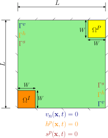
Figure 1. Quarter five-spot problem: Pictorial description of the problem including initial and boundary conditions. The computational domain includes a unit square ($L=1$) and two small squares with length $W$. The bottom left corner square ($\Omega^{I}$) is injection well and the top right one ($\Omega^{P}$) is production well.

We alter the quarter five-spot problem, used often in studies on flow through porous media, to fit the studies on double-diffusive effects. Figure 1 provides a pictorial description of the problem. The computational domain is a square with length $L=1$. There are also two small squares of length $W=L/10$ near the bottom left, the injection well $\Omega^{I}$, and top right, the production well $\Omega^{P}$, corners. One needs to introduce small perturbations into the prescribed data (e.g., initial condition, medium properties like permeability, or boundary conditions) to trigger physical instabilities like the viscous fingers. Instead, one can introduce a chemical reaction into transport equations, resulting in advection-diffusion-reaction (ADR) equations, to trigger physical instabilities. In the studies presented in this section, we introduce a chemical reaction in both transport and thermal subproblems near the production well ($\Omega^{P}$) to trigger viscous fingers.

From the injection well of $\Omega^{I}$, displacing fluid mass ($\varphi^{I}$) is injected into the domain which is already filled by displaced fluid at rest. The top right square ($\Omega^{P}$) is production well that has mass sink ($\varphi^{P}$). Elsewhere, $\varphi^{I}=\varphi^{P}=0$. Homogeneous velocity is enforced on the entire boundary (i.e., $v_{n}(\mathbf{x},t)=0\;\mathrm{on}\;\partial\Omega\times]0,\mathcal{I}[$). The zero fluxes are prescribed on the entire boundary for ADR equations (i.e., $h^{\mathrm{p}}(\mathbf{x},t)=0\;\mathrm{on}\;\partial\Omega\times]0,\mathcal{I}[$) and heat equations (i.e., $s^{\mathrm{p}}(\mathbf{x},t)=0\;\mathrm{on}\;\partial\Omega\times]0,\mathcal{I}[$). As before, the viscosity depends exponentially on the concentration and temperature. That is, $\mu=\mu_{0}\exp\left[R_{c}(1-c)+R_{\theta}(1-\theta)\right]$. The injection source and production sink are $\varphi^{I}=\varphi^{P}=0.1$, respectively. The maximum principle implies that the concentration field should lie between 0 and 1; that is, $0\leq c(\mathbf{x},t)\leq 1$.

Table 1. Quarter five-spot: Parameters used in the problem.

Parameter	Value
$d_{m}$	$10^{-7}$
$f(\mathbf{x},t)$	$\varphi^{I}\;\;\mathrm{in}\;\;\Omega^{I}$
$r(\mathbf{x},t,c)$	$-\varphi^{P}c\;\;\mathrm{in}\;\;\Omega^{P}$
$g(\mathbf{x},t)$	$\varphi^{I}\;\;\mathrm{in}\;\;\Omega^{I}$
$q(\mathbf{x},t,\theta)$	$-\varphi^{P}\theta\;\;\mathrm{in}\;\;\Omega^{P}$
$R_{c}$	2
$R_{\theta}$	2
$\mu_{0}$	1

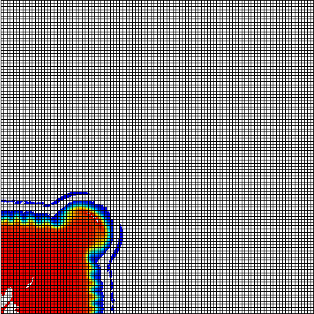
(a) SUPG at $t=100$

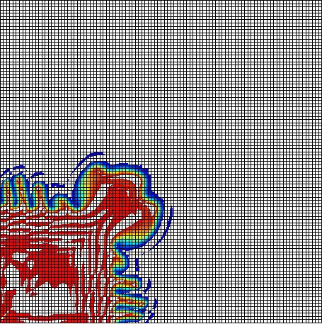
(b) SUPG at $t=175$

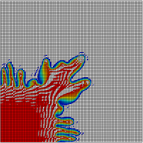
(c) SUPG at $t=250$

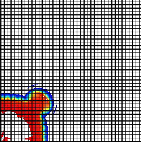
(d) SUPG + isotropic diffusion at $t=100$

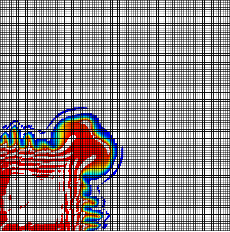
(e) SUPG + isotropic diffusion at $t=175$

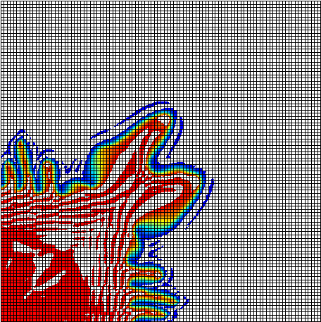
(f) SUPG + isotropic diffusion at $t=250$

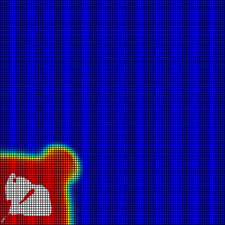
(g) SUPG + crosswind diffusion at $t=100$.

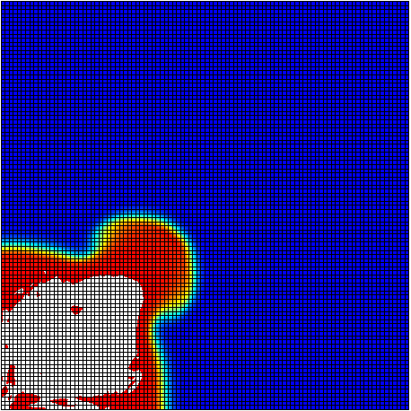
(h) SUPG + crosswind diffusion at $t=175$

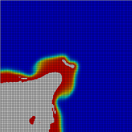
(i) SUPG + crosswind diffusion at $t=250$

Figure 2. Violation of the maximum principle: These figures show concentration at different time steps for coupled flow, ADR and temperature equations under numerical stabilizers. The upper figures are for SUPG formulation (equation (3.1.1)). the middle figures are for modified SUPG in which we added isotropic artificial diffusion (equation (3.7)) and bottom figures are for modified SUPG with crosswind artificial diffusion (equation (3.8)). The results are obtained for parameters provided in Table 1. The white regions represent the regions in which the concentration has violated the maximum principle. The injection source and production sink are $\varphi^{I}=\varphi^{P}=0.1$. The mesh used for this problem is $100\times 100$ structured quadrilateral elements. The numerical results clearly violate the maximum principle (and in consequence non-negative constraint) for the concentration.

We performed numerical simulations using the SUPG formulation and its modifications, got by adding one or both of the isotropic and crosswind artificial diffusion terms to the SUPG formulation. We have used $100\times 100$ quadrilateral finite elements. Table 1 provides the parameters used in the numerical simulation. Figure 2 shows the concentration profiles at time levels $t=100,175$ and $250$ for three cases: the SUPG formulation, SUPG with isotropic diffusion, and SUPG with crosswind diffusion. The numerical solutions for the concentration field under all the three cases did not remain in the range $[0,1]$, and they violated the maximum principle and the non-negative constraint for all the three cases. For instance, at $t=250$, the concentration field under the SUPG formulation is $-2.75\leq c\leq 6.21$; see Figure 3.

Figure 3. Violation of maximum principle: These figures show unphysical concentration values at time $t=250$ for the quarter five-spot problem under the SUPG stabilized formulation. The parameters for these figures are the same as those used for Figure 2.

Since adding a stabilizer one at a time—either isotropic diffusion or crosswind diffusion—did not eliminate spurious oscillations, we have solved the same problem by adding both the stabilizers to the SUPG formulation. Figure 4 shows the corresponding results for the concentration field. Although adding both the stabilizers have eliminated numerical instabilities (spurious oscillation, and the violations of the maximum principle and the non-negative constraint), it also suppressed physical hydrodynamic instabilities. That is, we did not observe VF under the SUPG formulation with isotropic and crosswind diffusion stabilizers.

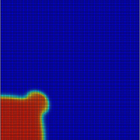
(a) $t=100$

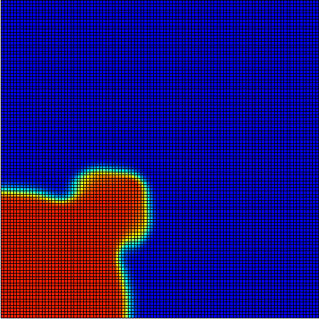
(b) $t=175$

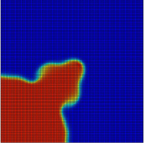
(c) $t=250$

Figure 4. Suppression of physical instabilities: These figures show concentration profiles at various time levels for the quarter five-spot problem under the modified SUPG stabilized formulation with isotropic and crosswind artificial diffusion stabilizers. The parameters for these figures are the same as those used for Figure 2. Although the results satisfy the maximum principle and the non-negative constraint for the concentration field, the utilized stabilizers suppress physical instabilities (i.e., the fingers).

5. CLOSURE

We have shown that numerical stabilization techniques, which aim at removing spurious oscillations in the concentration and temperature profiles, may suppress physical instabilities (such as VF). Several popular stabilized formulations violate the non-negative constraint and the maximum principle for the concentration field. Several prior studies have reported such violations for the cases of advection-diffusion and VF with the single diffusivity under dispersion tensors with strong anisotropy (e.g., see [Chang and Nakshatrala, 2017]). However, we reported that such violations could occur even under isotropic diffusivity for VF with DD effects.

The research reported in this paper highlights two points. First, practitioners who use existing numerical formulations should be wary of possible inaccurate and unphysical results when dealing with physical instabilities. They must choose with caution an appropriate numerical method that suppresses unphysical oscillations and captures physical instabilities at the same time. Second, there is a need to develop new robust numerical formulations for coupled flow-transport problems, and in particular, to simulate double-diffusive effects. The non-negative formulations based on variational inequality, developed for coupled flow-transport problems with single diffusive effects [Chang and Nakshatrala, 2017] and flow through porous media problems [Mapakshi et al., 2018], could provide a viable route for developing numerical formulations for double-diffusive effects.

References

- Augustin et al. [2011] M. Augustin, A. Caiazzo, A. Fiebach, J. Fuhrmann, V. John, A. Linke, and R. Umla. An assessment of discretizations for convection-dominated convection–diffusion equations. Computer Methods in Applied Mechanics and Engineering, 200:3395–3409, 2011.
- Brezzi and Fortin [1991] F. Brezzi and M. Fortin. Mixed and Hybrid Finite Element Methods, volume 15 of Springer series in computational mathematics. Springer-Verlag, New York, USA, 1991.
- Brooks and Hughes [1982] A. N. Brooks and T. J. R. Hughes. Streamline upwind/Petrov-Galerkin methods for convection dominated flows with emphasis on the incompressible Navier-Stokes equations. Computer Methods in Applied Mechanics and Engineering, 32:199–259, 1982.
- Chan and Liang [1997] C. K. Chan and N. Y. Liang. Observations of surfactant driven instability in a Hele-Shaw cell. Physical Review Letters, 79:4381, 1997.
- Chang and Nakshatrala [2017] J. Chang and K. B. Nakshatrala. Variational inequality approach to enforcing the non-negative constraint for advection–diffusion equations. Computer Methods in Applied Mechanics and Engineering, 320:287–334, 2017.
- Chang and Slattery [1986] S-H. Chang and J. C. Slattery. A linear stability analysis for miscible displacements. Transport in Porous Media, 1:179–199, 1986.
- Chen and Meiburg [1998] C-Y. Chen and E. Meiburg. Miscible porous media displacements in the quarter five-spot configuration. Part 2. Effect of heterogeneities. Journal of Fluid Mechanics, 371:269–299, 1998.
- de Bruyn [1995] J. R. de Bruyn. Fingering instability of gravity currents in thin-layer electrochemical deposition. Physical Review Letters, 74:4843, 1995.
- Evans [1998] L. C. Evans. Partial Differential Equations. American Mathematical Society, Providence, Rhode Island, 1998.
- Fernandez and Homsy [2003] J. Fernandez and G. M. Homsy. Viscous fingering with chemical reaction: effect of in-situ production of surfactants. Journal of Fluid Mechanics, 480:267–281, 2003.
- Gilbarg and Trudinger [2001] D. Gilbarg and N. S. Trudinger. Elliptic Partial Differential Equations of Second Order. Springer, New York, 2001.
- Gresho and Sani [2000] P. M. Gresho and R. L. Sani. Incompressible Flow and the Finite Element Method: Advection-Diffusion. John Wiley & Sons, Inc., Chichester, 2000.
- Hejazi et al. [2010] S. H. Hejazi, P. M. J. Trevelyan, J. Azaiez, and A. De Wit. Viscous fingering of a miscible reactive interface: A linear stability analysis. Journal of Fluid Mechanics, 652:501–528, 2010.
- Hughes et al. [1986] T. J. R. Hughes, M. Mallet, and M. Akira. A new finite element formulation for computational fluid dynamics: II. Beyond SUPG. Computer Methods in Applied Mechanics and Engineering, 54:341–355, 1986.
- Islam and Azaiez [2010a] M. N. Islam and J. Azaiez. Miscible thermo-viscous fingering instability in porous media. Part 1: Linear stability analysis. Transport in Porous Media, 84:821–844, 2010a.
- Islam and Azaiez [2010b] M. N. Islam and J. Azaiez. Miscible thermo-viscous fingering instability in porous media. Part 2: Numerical simulations. Transport in Porous Media, 84:845–861, 2010b.
- John and Knobloch [2007] V. John and P. Knobloch. On spurious oscillations at layers diminishing (SOLD) methods for convection–diffusion equations: Part I – A review. Computer Methods in Applied Mechanics and Engineering, 196:2197–2215, 2007.
- Johnson et al. [1987] C. Johnson, A. H. Schatz, and L. B. Wahlbin. Crosswind smear and pointwise errors in streamline diffusion finite element methods. Mathematics of Computation, 49:25–38, 1987.
- Karimi and Nakshatrala [2016] S. Karimi and K. B. Nakshatrala. Do current lattice Boltzmann methods for diffusion-type equations respect maximum principles and the non-negative constraint? Communications in Computational Physics, 20:374–404, 2016.
- Li and Rivière [2015] J. Li and B. Rivière. Numerical solutions of the incompressible miscible displacement equations in heterogeneous media. Computer Methods in Applied Mechanics and Engineering, 292:107–121, 2015.
- Liska and Shashkov [2008] R. Liska and M. Shashkov. Enforcing the discrete maximum principle for linear finite element solutions of second-order elliptic problems. Communications in Computational Physics, 3:852–877, 2008.
- Maes et al. [2010] R. Maes, G. Rousseaux, B. Scheid, M. Mishra, P. Colinet, and A. De Wit. Experimental study of dispersion and miscible viscous fingering of initially circular samples in Hele-Shaw cells. Physics of Fluids, 22:123104, 2010.
- Mapakshi et al. [2018] N. K. Mapakshi, J. Chang, and K. B. Nakshatrala. A scalable variational inequality approach for flow through porous media models with pressure-dependent viscosity. Journal of Computational Physics, 359:137–163, 2018.
- Mishra et al. [2010] M. Mishra, P. M. J. Trevelyan, C. Almarcha, and A. De Wit. Influence of double diffusive effects on miscible viscous fingering. Physical Review Letters, 105:204501, 2010.
- Nagarajan and Nakshatrala [2010] H. Nagarajan and K. B. Nakshatrala. Enforcing the non-negativity constraint and maximum principles for diffusion with decay on general computational grids. International Journal for Numerical Methods in Fluids, In print, DOI: 10.1002/fld.2389, 2010.
- Nagatsu et al. [2009] Y. Nagatsu, N. Fujita, Y. Kato, and Y. Tada. An experimental study of non-isothermal miscible displacements in a Hele-Shaw cell. Experimental Thermal and Fluid Science, 33:695–705, 2009.
- Nakshatrala et al. [2013] K. B. Nakshatrala, M. K. Mudunuru, and A. J. Valocchi. A numerical framework for diffusion-controlled bimolecular-reactive systems to enforce maximum principles and the non-negative constraint. Journal of Computational Physics, 253:278–307, 2013.
- Nakshatrala et al. [2016] K. B. Nakshatrala, H. Nagarajan, and M. Shabouei. A numerical methodology for enforcing maximum principles and the non-negative constraint for transient diffusion equations. Communications in Computational Physics, 19:53–93, 2016.
- Potier [2005] C. Le Potier. Finite volume monotone scheme for highly anisotropic diffusion operators on unstructured triangular meshes. Comptes Rendus Mathematique, 341:787–792, 2005.
- Pritchard [2004] D. Pritchard. The instability of thermal and fluid fronts during radial injection in a porous medium. Journal of Fluid Mechanics, 508:133–163, 2004.
- Pritchard [2009] D. Pritchard. The linear stability of double-diffusive miscible rectilinear displacements in a Hele-Shaw cell. European Journal of Mechanics-B/Fluids, 28:564–577, 2009.
- Raghavan and Marsden [1971] R. Raghavan and S. S. Marsden. The stability of immiscible liquid layers in a porous medium. Journal of Fluid Mechanics, 48:143–159, 1971.
- Riaz and Tchelepi [2004] A. Riaz and H. A. Tchelepi. Linear stability analysis of immiscible two-phase flow in porous media with capillary dispersion and density variation. Physics of Fluids, 16:4727–4737, 2004.
- Riaz and Tchelepi [2006] A. Riaz and H. A. Tchelepi. Numerical simulation of immiscible two-phase flow in porous media. Physics of Fluids, 18:014104, 2006.
- Saffman [1986] P. G. Saffman. Viscous fingering in Hele-Shaw cells. Journal of Fluid Mechanics, 173:73–94, 1986.
- Saffman and Taylor [1958] P. G. Saffman and G. Taylor. The penetration of a fluid into a porous medium or Hele-Shaw cell containing a more viscous liquid. Proceedings of the Royal Society of London A, 245:312–329, 1958.
- Scovazzi et al. [2013] G. Scovazzi, H. Huang, S. S. Collis, and J. Yin. A fully-coupled upwind discontinuous Galerkin method for incompressible porous media flows: High-order computations of viscous fingering instabilities in complex geometry. Journal of Computational Physics, 252:86–108, 2013.
- Tan and Homsy [1986] C. T. Tan and G. M. Homsy. Stability of miscible displacements in porous media: Rectilinear flow. Physics of Fluids, 29:3549–3556, 1986.
- Tan and Homsy [1988] C. T. Tan and G. M. Homsy. Simulation of nonlinear viscous fingering in miscible displacement. Physics of Fluids, 31:1330–1338, 1988.
- Tan and Homsy [1992] C. T. Tan and G. M. Homsy. Viscous fingering with permeability heterogeneity. Physics of Fluids, 4:1099–1101, 1992.
- Taylor [1950] G. Taylor. The instability of liquid surfaces when accelerated in a direction perpendicular to their planes. I. Proceedings of the Royal Society of London A: Mathematical, Physical and Engineering Sciences, 201:192–196, 1950.
- Tchelepi et al. [1993] H. A. Tchelepi, F. M. Orr, N. Rakotomalala, D. Salin, and R. Woumeni. Dispersion, permeability heterogeneity, and viscous fingering: Acoustic experimental observations and particle-tracking simulations. Physics of Fluids, 5:1558–1574, 1993.
- Wooding and Morel-Seytoux [1976] R. A. Wooding and H. J. Morel-Seytoux. Multiphase fluid flow through porous media. Annual Review of Fluid Mechanics, 8:233–274, 1976.
- Zik et al. [1998] O. Zik, Z. Olami, and E. Moses. Fingering instability in combustion. Physical Review Letters, 81:3868, 1998.
- Zimmerman and Homsy [1992a] W. B. Zimmerman and G. M. Homsy. Three-dimensional viscous fingering: A numerical study. Physics of Fluids, 4:1901–1914, 1992a.
- Zimmerman and Homsy [1992b] W. B. Zimmerman and G. M. Homsy. Viscous fingering in miscible displacements: Unification of effects of viscosity contrast, anisotropic dispersion, and velocity dependence of dispersion on nonlinear finger propagation. Physics of Fluids, 4:2348–2359, 1992b.