Transition polynomial as a weight system for binary delta-matroids

Abstract

To a singular knot $K$ with $n$ double points, one can associate a chord diagram with $n$ chords. A chord diagram can also be understood as a $4$-regular graph endowed with an oriented Euler circuit. L. Traldi introduced a polynomial invariant for such graphs, called a transition polynomial. We specialize this polynomial to a multiplicative weight system, that is, a function on chord diagrams satisfying $4$-term relations and determining thus a finite type knot invariant. We prove a similar statement for the transition polynomial of general ribbon graphs and binary delta-matroids defined by R. Brijder and H. J. Hoogeboom, which defines, as a consequence, a finite type invariant of links.

Перевод аннотации

Особому узлу $K$ с $n$ двойными точками сопоставляется хордовая диаграмма с $n$ хордами. Хордовую диаграмму можно также понимать как 4-регулярный граф с выделенным ориентированным эйлеровым циклом. Л. Тральди ввел инвариант таких графов, называемый многочленом переходов. Выбирая специальные параметры, мы превращаем этот многочлен в весовую систему, то есть функцию на хордовых диаграммах, которая удовлетворяет четырёхчленному соотношению, а значит определяет инвариант узлов конечного типа. Аналогичное утверждение мы доказываем и для многочлена переходов общих вложенных графов и бинарных дельта-матроидов, введенного Р. Брийдером и Х. Хугебумом, определяя, тем самым, инвариант зацеплений конечного типа.

Short title

Transition polynomial as a weight system

List of key words or phrases

knot, link, finite type invariant of knots, chord diagram, transition polynomial, delta-matroid.

2010 Mathematics Subject Classification

05C31 Graph polynomials

1 Introduction

A chord diagram of order $n$ is an oriented circle with $2n$ distinct points on it, split into $n$ disjoint pairs and considered up to orientation preserving diffeomorphisms of the circle. A function on chord diagrams is a weight system provided it satisfies Vassiliev’s $4$-term relations (see precise definitions in the next section). Vassiliev has shown that functions on chord diagrams with $n$ chords obtained from knot invariants of order at most $n$ satisfy the $4$-term relations, and Kontsevich proved that these are essentially the only restrictions, that is, a knot invariant is associated to each weight system.

We start with the following construction.

First, by contracting each chord of a chord diagram to a vertex, we make the diagram into a $4$-regular graph, that is, a graph in which all the vertices are $4$-valent. The set of vertices of this graph is in one-to-one correspondence with the set of chords in the initial chord diagram. The graph is also endowed with a distinguished oriented Euler circuit, which is the supporting circle of the chord diagram.

To such a pair (namely, a $4$-regular graph with an oriented Euler circuit), L. Traldi associates the weighted transition polynomial. This polynomial depends on three parameters, denoted $s,t$, and $u$. Our first main result consists in showing that for $u=-t$ the weighted transition polynomial is a weight system (taking values in the polynomial ring ${\mathbb{C}}[s,t,x]$, the variable $x$ being the argument of the transition polynomial).

A chord diagram also can be interpreted as an embedded graph with a single vertex. More generally, to a singular link one associates an embedded graph with several vertices, whose number equals the number of connected components of the link. Our second main result is that the transition polynomial for delta-matroids defined in [2] satisfies, after the same specialization, the $4$-term relations for binary delta-matroids introduced in [5] and defines thus a finite type invariant of links.

The paper is organized as follows.

In Section 2 we introduce the required definitions and formulate the main result for chord diagrams. Section 3 is devoted to its proof. Section 4 is devoted to the construction of an extension of the transition polynomial to arbitrary embedded graphs. We finish with constructing an extension of our invariant to binary delta-matroids.

The authors are grateful to Sergei Lando for the advice to study the theory of Vassiliev knot invariants and for pointing out the construction of Lorenzo Traldi in connection with them. This article wouldn’t appear without his advice. The authors also are grateful to unknown referee for useful comments allowing them to seriously improve presentation.

2 Definitions and statement of the main result

2.1 Chord diagrams and weight systems

A chord diagram of order $n$ is an oriented circle with $2n$ distinct points on it, split into $n$ disjoint pairs and considered up to orientation preserving diffeomorphisms of the circle. A function $f$ on chord diagrams with values in a commutative ring is called a weight system if it satisfies the $4$-term relations shown in Fig. 1. Here we pick a chord diagram $C$ and two chords with neighboring ends in it, and construct the other three diagrams as shown. All the four circles are assumed to be oriented counterclockwise. The four diagrams in the picture may contain other chords with the ends on the dotted arcs, which are the same for all four of them. An equivalent way to look at this is to consider functions on the vector space $M$ spanned by all chord diagrams over the field ${\mathbb{C}}$ factored over all $4$-term relations. The vector space $M$ has a ring structure. In order to multiply two chord diagrams, $C_{1}$ and $C_{2}$, we cut the supporting circle of each diagram at an arbitrary point different from the endpoints of the chords and glue the resulting arcs together to form a new supporting circle in an orientation-preserving way as it is done in Fig. 2. Modulo $4$-term relations, the result does not depend on the way we have chosen the cutting points. For the basics of Vassiliev knot invariants we refer the reader to Chapter 6 in the book by S. Lando and A. Zvonkin [6].

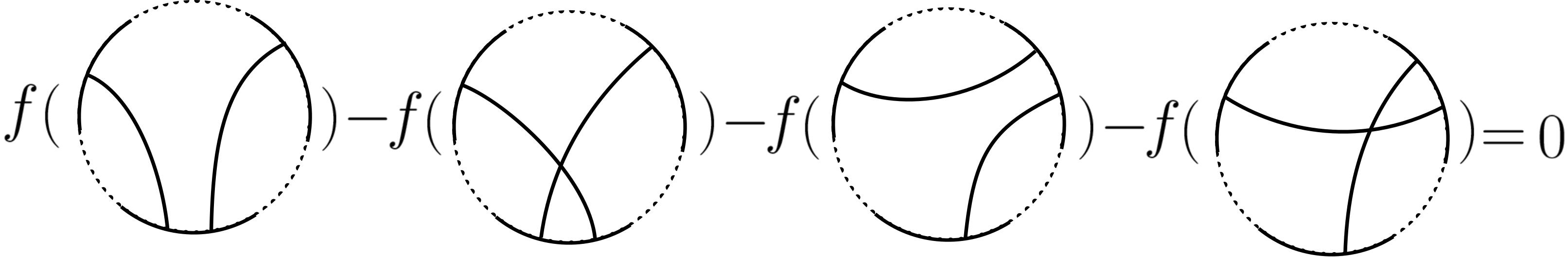
Рис. 1: 4-term relation

Рис. 2: Multiplication of chord diagrams

2.2 4-regular graphs, Greek labelings, and weighted transition polynomials

As discussed above, a 4-regular graph $G$ is a graph in which each vertex is 4-valent. By contracting the chords of a chord diagram $C$, we make it into a $4$-regular graph $G=G(C)$ endowed with an oriented Euler circuit. In this paper, we will look at an oriented Euler circuit from two points of view. Firstly, we may interpret an Euler circuit as a sequence of half-edges $h_{1}$, $h_{2}$, … , $h_{4n}$ considered up to cyclic permutations of its entries, where $n$ is the number of vertices in $G$, such that

1. Each half-edge enters the sequence once and two half-edges with consecutive indices either belong to the same edge or are incident to the same vertex.

2. If $h_{k}$ and $h_{k+1}$ belong to the same edge, then $h_{k+1}$ and $h_{k+2}$ are incident to the same vertex.

3. If $h_{k}$ and $h_{k+1}$ are incident to the same vertex, then $h_{k+1}$ and $h_{k+2}$ belong to the same edge.

The second way to look at an oriented Euler circuit is to say that it is an immersion of the standard oriented circle to $G$ such that each point of $G$ except the vertices has exactly one pre-image and each vertex has two pre-images. This construction is considered up to homotopy in the class of such maps.

2.2.1 Transitions and their Greek labeling

Let $G$ be a 4-regular graph and let $K$ be an oriented Euler circuit in it. At each vertex $v$ of $G$, there are 4 half-edges incident to $v$. They form the set $H(v)$. There are three ways to split $H(v)$ into two disjoint $2$-element subsets. These three partitions form the set $T(v)$, its elements are called the transitions at $v$. The Euler circuit $K$ allows us to assign a type to any transition. We will mark the types with the Greek letters $\phi$, $\chi$ and $\psi$.

Pick one of the two half-edges entering $v$ (we call this half-edge the starting one); choosing a pair for this half-edge determines the transition completely. There are three cases. If the pair to the starting half-edge is the one that follows it immediately along the Euler circuit, then we say that this transition belongs to type $\phi$, if it is the other leaving half-edge, then this is a $\chi$-transition and if it is the other entering half-edge, then this is a $\psi$-transition as illustrated in Fig. 3 (the letter ‘o’ denotes the starting half-edge). Note that if we choose the other half-edge entering $v$ for the starting one, then the types of the transitions will be the same.

Рис. 3: The Greek labeling of transitions (on the left) with respect to the specified Euler circuit (on the right)

2.2.2 Weighted transition polynomials

A circuit partition $P$ of a 4-regular graph $G$ with $n$ vertices is an $n$-tuple of transitions, one at each vertex. Given a circuit partition $P$ of $G$, we first erase all the vertices of $G$ and then we glue in pairs the free ends of half-edges that were paired in some transition from $P$. Since we have taken one transition at each vertex of $G$, each half-edge of $G$ participates exactly once in a transition from $P$ and we obtain a disjoint family of circles. Let their number be $c(P)$. Let ${\cal P}(G)$ be the set of all circuit partitions of $G$. The set of all transitions of $G$ is denoted by ${\cal T}(G)$. A weight function is a map from ${\cal T}(G)$ to a commutative ring. For a given weight function $w$, the weighted transition polynomial $Q_{w}$ is the sum of the monomials that correspond to circuit partitions of $G$. The monomial for a given circuit partition $P$ is $x^{c(P)-1}$ times the product of the weights of all transitions in $P$, so that

$$Q_{w}(G)=\sum_{P\in P(G)}\prod_{v\in V(G)}w(T(v)\cap P)x^{c(P)-1}.$$

The weighted transition polynomial was introduced by F. Jaeger [4].

2.3 Statement of the first main theorem

If we define the weight function in such a way that it takes on a transition values depending only on the type $\phi,\psi$, or $\chi$ of the transition, then we obtain Traldi’s transition polynomial. In this section, we introduce the function $Q$ taking chord diagrams to elements of ${\mathbb{C}}[s,t,x]$ as a specialization of Traldi’s transition polynomial. Its value on a chord diagram $C$ is the weighted transition polynomial of the corresponding $4$-regular graph $G(C)$. We attach to transitions in $G$ weights according to their types with respect to $E(D)$. All the $\phi$-transitions are assigned the weight $s$, all the $\psi$-transitions are assigned the weight $t$, and all the $\chi$-transitions are assigned the weight $-t$.

Theorem 2.1

The function $Q$ is a multiplicative weight system.

3 Proof of Theorem 2.1

Instead of counting the number of connected components in a circuit partition $P$ of a $4$-regular graph $G(C)$ with an oriented Euler circuit $K=K(C)$, we can count the number of connected components of the boundary of the ribbon graph with one vertex corresponding to the chord diagram $C$ and the partition $P$. Let $P$ be a circuit partition. Assign the corresponding Greek letters to the chords of the chord diagram $C$; such a marked chord diagram will be denoted by $C(P)$. Associate to the marked chord diagram $C(P)$ the ribbon graph $R(P)$ by attaching the disc to the supporting circle of $C$ and replacing every chord with marking $\chi$ by a ribbon, every chord with marking $\psi$ by a half-twisted ribbon, and erasing every chord with marking $\phi$.

The value of the function $Q$ on a chord diagram with $n$ chords is a sum of $3^{n}$ monomials. Each monomial corresponds to the choice of Greek letters at each of the chords. Figure 4 shows how the value of $\Psi$ on a chord diagram is constructed, for a chosen chord and all its possible markings with the Greek letters, assuming the markings on all the other chords are fixed.

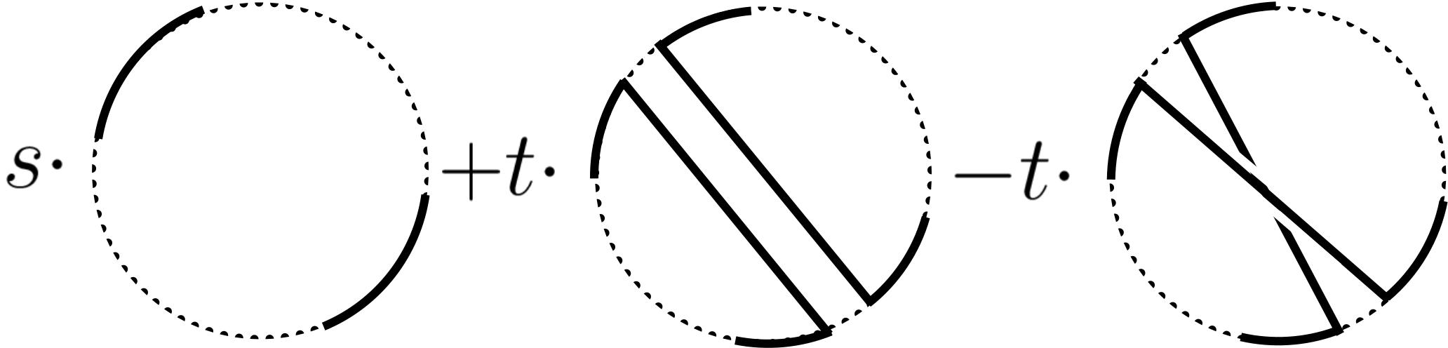
Рис. 4: Impact of the choices of the marks on a specific chord

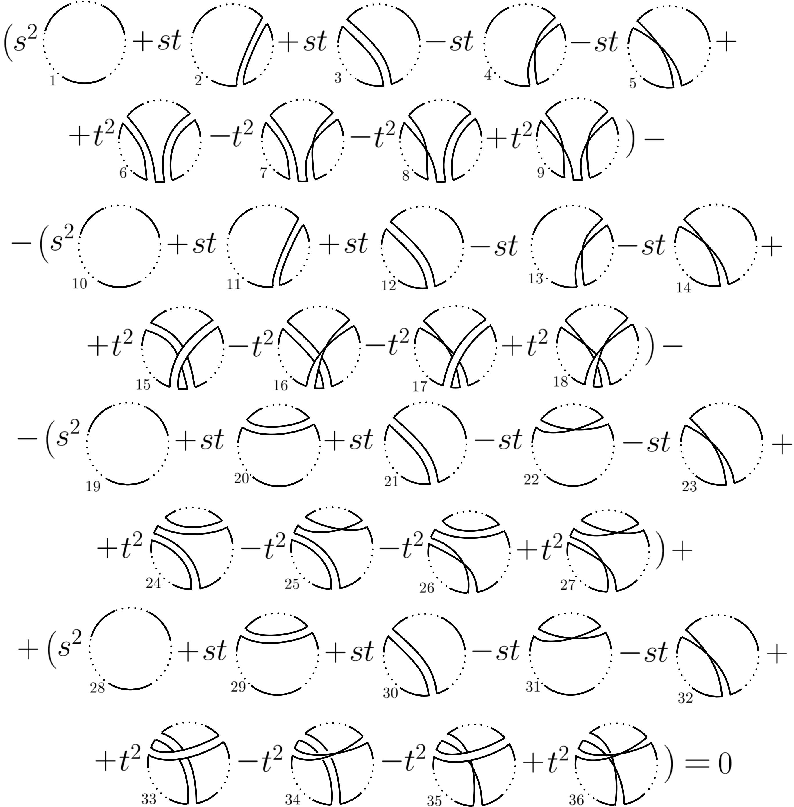
Рис. 5: Checking the $4$-term relation for $Q$

In Fig. 5, the $4$-term relation is checked. We take a chord diagram $C$ and pick two chords $a$ and $b$ with neighboring ends in it. We are going to show that the corresponding $4$-term relation is satisfied not just for the whole function $Q$, but for each subsum in it corresponding to a given choice of Greek letters for all chords but $a$ and $b$. Each bracket of the $4$-term expression contains 9 monomials in $Q$ and each monomial is the product of the weights of $a$ and $b$ and $x^{c(P)-1}$ where $c(P)$ is the number of connected components of the boundary of the ribbon graph associated to the partition $P$, times the product of the weights of all other chords, which are the same for all the $4$ terms. The summands are numbered (the number is shown in the brackets under the coefficient of the diagram with this number). The paired summands below differ only by the sign:

$$(1,10);(2,11);(3,12);(4,13);(5,14);(6,24);(7,25);$$

$$(8,36);(9,35);(15,33);(16,34);(17,27);(18,26);$$

$$(19,28);(20,29);(21,30);(22,31);(23,32)$$

For the first five pairs, it is obvious that the two paired ribbon graphs are homeomorphic to one another and hence have the same number of connected components of the boundary. For the pairs from 6 to 9, the second ribbon graph in the pair could be obtained from the first one after applying the handle sliding, which doesn’t change the topology of the ribbon graph. For the pairs 8 and 9, the handle $b$ slides through the twisted ribbon $a$ and twists because of that. For the rest of the pairs the proof is similar.

Theorem 2.1 is proved.

4 The extension of the $Q$-polynomial to ribbon graphs

Above, we restricted our attention to ribbon graphs with a single vertex in order to check the $4$-term relation for the $Q$-function on chord diagrams. From now on we omit this restriction and consider arbitrary ribbon graphs. We present a natural way to define the $Q$-polynomial on a ribbon graph $R$ as an analogous specification of a transition polynomial for a medial graph of $R$. Similarly to the case of chord diagrams, we attach a Greek letter to every ribbon (this data is denoted by $L$). Then we take the product of weights of all Greek letters in $L$ ($s$ for $\phi$, $t$ for $\chi$ and $-t$ for $\psi$) and $x^{c(R(L))-1}$, where $c(R(L))$ is the number of connected components of the boundary of the ribbon graph $R(L)$. The latter is constructed from $R$ by half-twisting all the ribbons endowed with the letter $\psi$ and erasing all the ribbons endowed with the letter $\phi$. The polynomial $Q$ is then defined as the result of the summation over all states $L$.

The $4$-term relation for ribbon graphs is shown in the upper row in Fig. 6. Here we pick a ribbon graph $R$ and two ribbons with neighboring ends in it, and construct the other three ribbon graphs as shown. The four ribbon graphs in the picture may contain other ribbons, which are the same for all four of them.

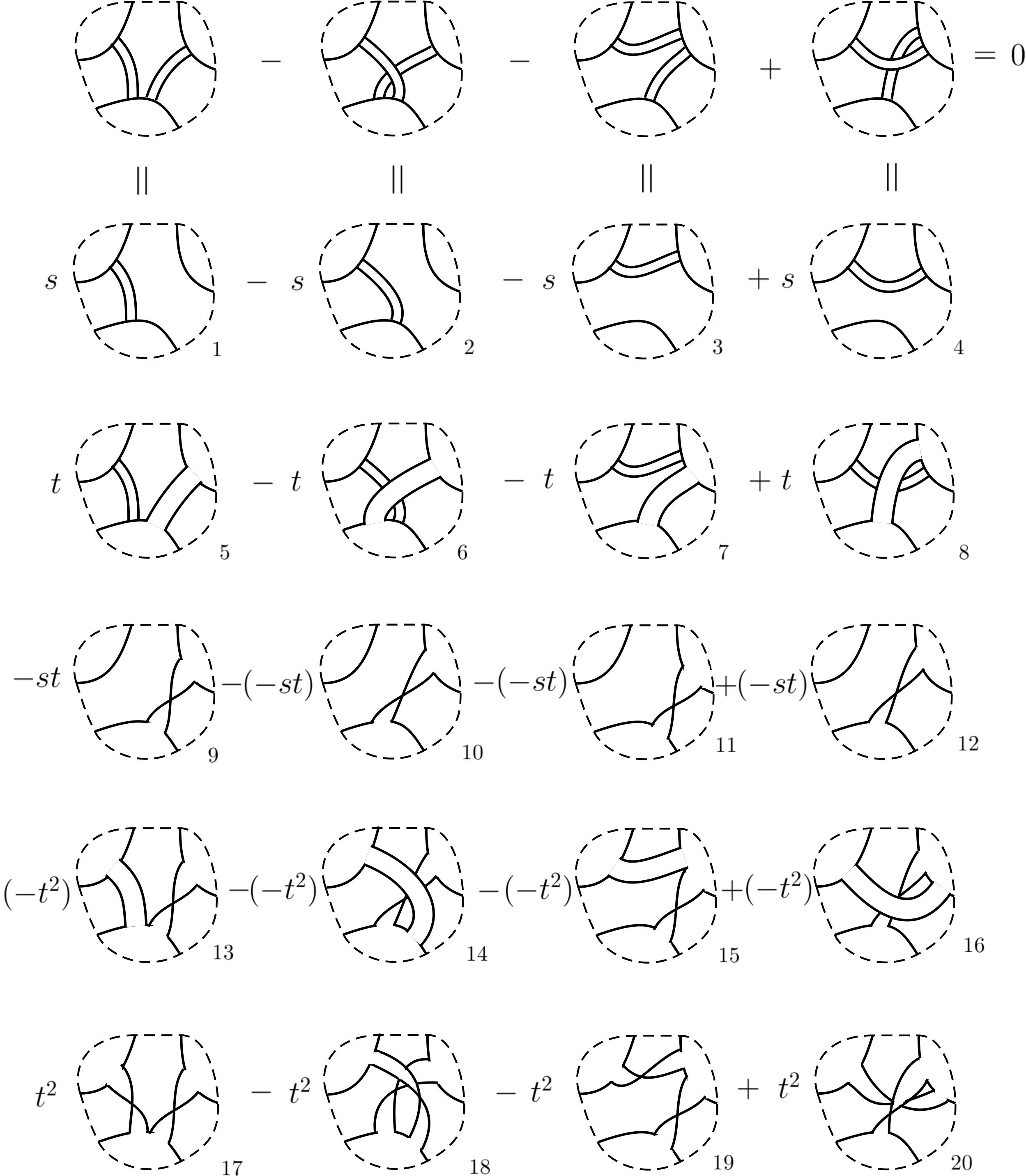
Рис. 6: Checking the 4-term relation for ribbon graphs

The 4-term relation for our polynomial on ribbon graphs is checked in the same way as it was done for chord diagrams, see Fig. 6.

5 Weighted transition polynomial for binary delta-matroids

In this section we study the weighted transition polynomial for binary $\bigtriangleup$-matroids. The notions of a $\bigtriangleup$-matroid and a binary $\bigtriangleup$-matroid were introduced by Bouchet [1]. Our presentation below follows that of [5], where the $4$-term relations and the Hopf algebra of binary delta-matroids were introduced.

Weighted transition polynomial $Q$ for delta-matroids (and, more generally, for arbitrary set systems) was defined in [2]. To each ribbon graph $R$, a binary delta-matroid $D(R)$ is associated. The polynomial $Q$ for binary delta-matroids possesses the property that $Q(D(R))=Q(R)$. We also prove that the 4-term relations for binary delta-matroids introduced in [5] are satisfied for the transition polynomial. We start with basic notions from the theory of delta-matroids. Then, following [2], we define the transition polynomial for binary delta-matroids and its specification $Q$, and prove that it satisfies the $4$-term relations.

5.1 Basics of delta-matroids

A set system is a pair $(E,S)$ where $E$ is a finite set and $S\subset 2^{E}$. The set $E$ is called the ground set and elements of $S$ are called feasible sets. Two set systems $(E_{1},S_{1})$ and $(E_{2},S_{2})$ are said to be isomorphic if there exists a bijection $f:E_{1}\rightarrow E_{2}$ such that $f(S_{1})=S_{2}$. Below, we do not distinguish between isomorphic set systems.

A delta-matroid is a set system $(E,S)$, with a non-empty $S$, satisfying the following Symmetric Exchange Axiom:

Axiom 1 (SEA)

For any two feasible sets $X$ and $Y$ and any $a\in X\bigtriangleup Y$ there is $b\in X\bigtriangleup Y$ (which is allowed to be equal to $a$) such that $X\bigtriangleup\{a,b\}$ is feasible (in the case $b=a$, $X\Delta\{a\}\in S$).

Here and below $\bigtriangleup$ denotes the symmetric difference operation on pairs of sets.

To any connected ribbon graph $R$, we assign a delta-matroid $D(R)=(E(R),S(R))$. Here $E(R)$ is the set of edges of $R$ and the feasible sets are those subsets of $E$ that induce a ribbon subgraph whose boundary consists of a single connected component.

To a simple graph $G$, the delta-matroid $D(G)=(E(G),S(G))$ is associated. The ground set $E(G)$ is the set of vertices of $G$, $E=V(G)$. A subset $A\subset E(G)$ is feasible if the adjacency matrix of the subgraph of $G$ induced by $A$ is nondegenerate over ${\mathbb{F}}_{2}$ (and empty set is feasible by definition). A delta-matroid $D$ is said to be graphic if there exists a graph $G$ such that $D=D(G)$.

Let $(E,S)$ be a $\bigtriangleup$-matroid and let $A\subset E$; then the partial duality $(E,S)*A$ of $(E,S)$ by the set $A$ is defined by $(E,S)*A=(E,\{F\subset E|F\bigtriangleup A\in S\})$. (If $A$ is a one-element set, $A=\{a\}$, we simply write $(E,S)*a$ instead of $(E,S)*\{a\}$).

A delta-matroid $D$ is said to be binary if there exists a graphic delta-matroid $D{{}^{\prime}}=(E,S)$ and a set $A\subset E$ such that $D=D{{}^{\prime}}*A=(E,S)*A$.

Remark 5.1

For a ribbon graph $R$, the delta-matroid $D(R)$ is a binary delta-matroid.

The following statement shows, in particular, that the delta-matroid of a ribbon graph with a single vertex coincides with the delta-matroid of the intersection graph of the corresponding chord diagram.

Theorem 5.1

Let $C$ be a chord diagram and let $\Gamma(C)$ be its intersection graph, $A(\Gamma(C))$ being its adjacency matrix over ${\mathbb{F}}_{2}$, then $corank(A(\Gamma(C)))={\rm bc}(C)-1$ where ${\rm bc}(C)$ is the number of boundary components of $C$.

Recall that the intersection graph $\Gamma(C)$ of a chord diagram $C$ is the graph whose vertices are in one-to-one correspondence with the chords of $C$, two vertices being connected by an edge iff the ends of the corresponding chords alternate along the circle. A proof of this theorem can be found in [7], [9], [10].

An element $a$ of a $\bigtriangleup$-matroid $(E,S)$ is a bridge if for each $F\in S$ we have $F\ni a$, and it is a loop if for any $F\in S$ we have $F\not\ni a$. These definitions mimic ones for ribbon graphs.

Let $(E,S)$ be a $\bigtriangleup$-matroid, and $a\in E$, then $(E,S){\setminus}a$ is the result of deleting $a$:

$$(E,S){\setminus}a=\begin{cases}(E\setminus\{a\},\{F\subset E\setminus\{a\}|F\in S\})&\text{if }a\text{ is not a bridge}\\ (E\setminus\{a\},\{F\subset E\setminus\{a\}|F\cup\{a\}\in S\})&\text{otherwise}\\ \end{cases}$$

We denote by $(E,S)/a$ the result of contracting $a$:

$$(E,S)/a=\begin{cases}(E\setminus\{a\},\{F\subset E\setminus\{a\}|F\cup\{a\}\in S\})&\text{if }a\text{ is not a loop}\\ (E\setminus\{a\},\{F\subset E\setminus\{a\}|F\in S\})&\text{otherwise}\\ \end{cases}$$

For a delta-matroid $D=(E,S)$, define the function $d_{D}$ on the subsets of its ground set by the formula $d_{D}(A)=\min_{F\in S}|A\Delta F|$. In addition, we denote by $d^{0}_{D}=d_{D}(\emptyset)$ the cardinality of a smallest feasible set.

Theorem 5.2

For a ribbon graph $R$, the number $d^{0}_{D(R)}+1$ coincides with the number of vertices of $R$.

Доказательство.

This statement follows from the fact that $D(R)*A$ is the delta-matroid of $R*A$ where $R*A$ is the partial duality of $R$ by the set $A$, see [3]. In order to obtain a ribbon graph with one vertex, we need to take for $A$ a set containing a spanning tree on the vertices of $R$. The number of edges in this tree is one less than $d^{0}_{D(R)}$. ∎

The number ${\rm bc}(D)$ of connected components of the boundary of a delta-matroid $D=(E,S)$ is the minimal $n\in\mathbb{N}$ possessing the property that there exists a set $A\subset E$ of cardinality $n-1$ such that $D*(E\setminus A)$ is a graphic delta-matroid.

Remark 5.2

It is easy to see that $d^{0}_{D}={\rm bc}(D*E(D))$, where $E(D)$ is the ground set of $D$.

Corollary 5.1

Let $R$ be a connected ribbon graph, then ${\rm bc}(R)={\rm bc}(D(R))$.

Let $D=(E,S)$ be a binary delta-matroid, and let $a,b\in E$.

The result of sliding of the element $a$ over the element $b$ is the set system $\widetilde{D}_{ab}=(E;\widetilde{S}_{ab})$, where $\widetilde{S}_{ab}=S\Delta\{A\sqcup\{a\}|A\sqcup\{b\}\in S\text{ and }A\subset E{\setminus}\{a,b\}\}$.

This definition was given in [8] and interpreted as the second Vassiliev move in [5].

The result of exchanging the ends of the ribbons $a,b$ is the set system $D^{\prime}_{ab}=(E;S^{\prime}_{ab})$, where $S^{\prime}_{ab}=\widetilde{(S*b)}_{ab}*b$, and this is the first Vassiliev move.

Remark 5.3

If $b$ is a bridge, then $\widetilde{S}_{ab}=S$, and $S^{\prime}_{ab}=S$.

5.2 Transition polynomial for binary delta-matroids

In order to define the transition polynomial for binary delta-matriods, we need two more operations.

Let $D=(E,S)$ be a $\bigtriangleup$-matroid, and let $u\in E$ be an element of its ground set. Then let us define the loop complementation $D+u$ of $D$ on $u$ by the formula $D+u=(E,S\Delta\{F\cup u|F\in S,u\not\in F\})$.

Below, operations on set systems are assumed to be applied from left to right, so that, for example, $M+u\setminus u*v$ means $((M+u)\setminus u)*v.$

Define the dual pivot $D\overline{*}u$ of a $\bigtriangleup$-matroid $D$ with respect to an element $u$ by $D\overline{*}u=D+u*u+u=D*u+u*u$. Similarly, for a subset $A\subset E$ of the ground set, we set $D\overline{*}A=D+A*A+A=D*A+A*A$.

The following definition is a specialization of the definition of weighted transition polynomial for delta-matroids in [2].

For a $\Delta$-matroid $D$, we define its transition polynomial $Q(D)$ (with parameters $s,t,-t$) as

$$Q(D)=\sum_{E(D)=\Phi\sqcup X\sqcup\Psi}s^{|\Phi|}t^{|X|}(-t)^{|\Psi|}x^{d^{0}_{D+\Phi*X\overline{*}\Psi}},$$

where summation is carried over all disjoint partitions of the ground set $E$ of $D$ into three parts.

Our main result for delta-matroids is the following statement.

Theorem 5.3

For an arbitrary binary $\Delta$-matroid $D=(E,S)$ and arbitrary elements $a,b\in E$ in its ground set, we have

$$Q(D)-Q(D^{\prime}_{ab})-Q(\widetilde{D}_{ab})+Q(\widetilde{D}^{\prime}_{ab})=0$$ (1)

The proof will require the following statement (Lemma 11 in [2]).

Lemma 5.1

Let $M=(E,S)$ be a set system, and let $u$, $v\in E$ such that $u\not=v$. Then $M+u{\setminus}v=M{\setminus}v+u$, $M*u{\setminus}v=M{\setminus}v*u$, и $M+u{\setminus}u=M{\setminus}u$.

Proposition 5.1

Let $D$ be a $\Delta$-matroid and $u$ an element of its ground set, then $d^{0}_{D}=d^{0}_{D{\setminus}u}-1$ if $u$ is a bridge, and $d^{0}_{D}=d^{0}_{D{\setminus}u}$, otherwise.

Доказательство.

Let $F$ be a feasible set of minimal size for the delta-matroid $D$. If $u$ is a bridge, then $F\setminus u$ is a feasible set of minimal size for $D\setminus u$. If $u$ is not a bridge, then either $F\not\ni u$ and $F$ is a feasible set of minimal size for $D\setminus u$, or there exists a feasible set $F^{\prime}$ such that $F^{\prime}\not\ni u$; to find such an $F^{\prime}$ we can take any feasible set $F^{\prime\prime}\not\ni u$ and apply the SEA axiom to the sets $F,F^{\prime\prime}$ and the element $u$ of their symetric diffirence. Then for $F$ and $F^{\prime\prime}$ and $u$ in $F\Delta F^{\prime\prime}$, there is $w\in F\Delta F^{\prime\prime}$ such that $F^{\prime}=F\Delta\{u,w\}$ is feasible. The cardinality of $F^{\prime}$ cannot be less than that of $F$ by the assumption (the set $F$ is a feasible set of minimal size) and $F^{\prime}\not\ni u$. ∎

Lemma 5.2

Let $D$ be a binary $\Delta$-matroid and suppose $a,b,u\in E(D)$ are pairwise distinct elements of its ground set. Then if $u$ is a bridge for one of the $\Delta$-matroids in the set $\{D,D*a,D+a,D\overline{*}a,D^{\prime}_{ab},\widetilde{D}_{ab},\widetilde{D}^{\prime}_{ab}\}$, then it is a bridge for all of them.

Доказательство.

It is easy to see that all the operations in the lemma are involutions, whence we have to prove only sufficiency.

It follows from the definitions of the operations that it suffices to prove the statement only for the operations $D\mapsto D*a$, $D\mapsto D+a$, and $D\mapsto\widetilde{D}_{ab}$, which is obvious by definition. ∎

The next proposition is an immediate corollary of Proposition 5.1 and Lemma 5.2.

Proposition 5.2

For an arbitrary binary delta-matroid $D$ and pairwise distinct elements $a,b,u$ in its ground set, the operation $D\mapsto D\setminus u$ commutes with the first and the second Vassiliev moves on the elements $a,b$.

Lemma 5.3

For an arbitrary binary delta-matroid $D$ and pairwise distinct elements $a,b,u$ in its ground set, the operations $D\mapsto D*u$, $D\mapsto D+u$, $D\mapsto D\overline{*}u$ commute with the first and the second Vassiliev moves on the elements $a,b$.

Доказательство.

Since the second Vassiliev move is a composition of the first one and the operation $*$, it suffices to check commutativity of the operations $D\mapsto D*u$ and $D\mapsto D+u$ with the first Vassiliev move. We have

• for the pair $D^{\prime}_{ab}$ and $+u$, $D^{\prime}_{ab}=(E,S\Delta\{F\cup\{ab\}|F\in S,\{ab\}\not\subset F\})$, hence

  $$(D+u)^{\prime}_{ab} = (E,[S\Delta\{F\cup\{u\}|F\in S,\{u\}\not\subset F\}]\Delta$$

  $$\{F\cup\{a,b\}|F\in[S\Delta\{F\cup\{u\}|F\in S,\{u\}\not\subset F\}],\{a,b\}\not\subset F\})$$

  $$= S\Delta\{F\cup\{u\}|F\in S,\{u\}\not\subset F\}\Delta\{F\cup\{a,b\}|F\in S,\{a,b\}\not\subset F\}$$

  $$= D^{\prime}_{ab}+u;$$

• for the pair $D^{\prime}_{ab}$ and $*u$,

  $$(D*u)^{\prime}_{ab} = (E,[\{F\Delta u|F\in S\}]\Delta\{F\cup\{a,b\}|F\in[\{F\Delta u|F\in S\}],\{a,b\}\not\subset F\})$$

  $$= (E,[\{F|F\Delta u\in S\}]\Delta\{F\cup\{a,b\}|F\in[\{F|F\Delta u\in S\}],\{a,b\}\not\subset F\})$$

  $$= (E,\{F\Delta u|F\in[S\Delta{F^{\prime}\cup\{a,b\}|F^{\prime}\in S}]\})$$

  $$= D^{\prime}_{ab}*u.$$

∎

Now we can prove Theorem 5.3

Доказательство.

Let us pick a pair of distinct elements $a,b$ in the ground set $E$. For a disjoint partition $E\setminus\{a,b\}=\Phi\sqcup X\sqcup\Psi$, define the polynomial $Q_{\Phi,X,\Psi}(D)$ as

$$Q_{\Phi,X,\Psi}(D)=\sum_{\{x,y\}=E_{\phi}\sqcup E_{\chi}\sqcup E_{\psi}}s^{|E_{\phi}|}t^{|E_{\chi}|}(-t)^{|E_{\psi}|}x^{d^{0}_{D+E_{\phi}*E_{\chi}\overline{*}E_{\psi}}}.$$ (2)

Now, we have

$$Q(D) = \sum_{E(D){\setminus}\{a,b\}=\Phi\sqcup X\sqcup\Psi}s^{|\Phi|}t^{|X|}(-t)^{|\Psi|}Q_{\Phi,X,\Psi}(D+\Phi*X\overline{*}\Psi),$$

$$Q(D^{\prime}_{ab}) = \sum_{E(D){\setminus}\{a,b\}=\Phi\sqcup X\sqcup\Psi}s^{|\Phi|}t^{|X|}(-t)^{|\Psi|}Q_{\Phi,X,\Psi}(D^{\prime}_{ab}+\Phi*X\overline{*}\Psi),$$

$$Q(\widetilde{D}_{ab}) = \sum_{E(D){\setminus}\{a,b\}=\Phi\sqcup X\sqcup\Psi}s^{|\Phi|}t^{|X|}(-t)^{|\Psi|}Q_{\Phi,X,\Psi}(\widetilde{D}_{ab}+\Phi*X\overline{*}\Psi),$$

$$Q(\widetilde{D}^{\prime}_{ab}) = \sum_{E(D){\setminus}\{a,b\}=\Phi\sqcup X\sqcup\Psi}s^{|\Phi|}t^{|X|}(-t)^{|\Psi|}Q_{\Phi,X,\Psi}(\widetilde{D}^{\prime}_{ab}+\Phi*X\overline{*}\Psi)$$

Lemma 5.3 implies the following presentations, where the summations are carried over all partitions of the set $\{a,b\}$ into triples of disjoint subsets $\{a,b\}=E_{\phi}\sqcup E_{\chi}\sqcup E_{\psi}$:

$$Q_{\Phi,X,\Psi}(D+\Phi*X\overline{*}\Psi) = Q_{\Phi,X,\Psi}({D})$$

$$= \sum_{\{a,b\}=E_{\phi}\sqcup E_{\chi}\sqcup E_{\psi}}s^{|E_{\phi}|}t^{|E_{\chi}|}(-t)^{|E_{\psi}|}x^{d^{0}_{{D_{1}}+E_{\phi}*E_{\chi}\overline{*}E_{\psi}}},$$

$$Q_{\Phi,X,\Psi}(D^{\prime}_{ab}+\Phi*X\overline{*}\Psi) = Q_{\Phi,X,\Psi}({D_{1}}^{\prime}_{ab})$$

$$= \sum_{\{a,b\}=E_{\phi}\sqcup E_{\chi}\sqcup E_{\psi}}s^{|E_{\phi}|}t^{|E_{\chi}|}(-t)^{|E_{\psi}|}x^{d^{0}_{{D_{1}^{\prime}}_{ab}+E_{\phi}*E_{\chi}\overline{*}E_{\psi}}},$$

$$Q_{\Phi,X,\Psi}(\widetilde{D}_{ab}+\Phi*X\overline{*}\Psi) = Q_{\Phi,X,\Psi}(\widetilde{D_{1}}_{ab})$$

$$= \sum_{\{a,b\}=E_{\phi}\sqcup E_{\chi}\sqcup E_{\psi}}s^{|E_{\phi}|}t^{|E_{\chi}|}(-t)^{|E_{\psi}|}x^{d^{0}_{\widetilde{D_{1}}_{ab}+E_{\phi}*E_{\chi}\overline{*}E_{\psi}}},$$

$$Q_{\Phi,X,\Psi}(\widetilde{D}^{\prime}_{ab}+\Phi*X\overline{*}\Psi) = Q_{\Phi,X,\Psi}(\widetilde{D_{1}}^{\prime}_{ab})$$

$$= \sum_{\{a,b\}=E_{\phi}\sqcup E_{\chi}\sqcup E_{\psi}}s^{|E_{\phi}|}t^{|E_{\chi}|}(-t)^{|E_{\psi}|}x^{d^{0}_{\widetilde{D_{1}^{\prime}}_{ab}+E_{\phi}*E_{\chi}\overline{*}E_{\psi}}},$$

where $D_{1}=D+\Phi*X\overline{*}\Psi$.

It is therefore sufficient to show that for any partition of the set $E(D)\setminus\{a,b\}$ into disjoint sets $\Phi$, $X$ and $\Psi$, the equation

$$Q_{\Phi,X,\Psi}(D)-Q_{\Phi,X,\Psi}({D}^{\prime}_{ab})-Q_{\Phi,X,\Psi}(\widetilde{D}_{ab})+Q_{\Phi,X,\Psi}(\widetilde{D}^{\prime}_{ab})=0$$ (3)

holds. By Proposition 5.1 and Proposition 5.2), the latter equation is equivalent (for an arbitrary $u\not\in\{x,y\}$) to the equation

$$Q_{\Phi,X,\Psi}(D{\setminus}u)-Q_{\Phi,X,\Psi}((D{\setminus}u)^{\prime}_{ab})-Q_{\Phi,X,\Psi}(\widetilde{D{\setminus}u}_{ab})+Q_{\Phi,X,\Psi}(\widetilde{(D{\setminus}u)}^{\prime}_{ab})=0$$

Therefore, we need to prove Eq.(3) only for delta-matroids with the ground set $\{x,y\}$. For any such delta-matrod $D$, there exists a ribbon graph $R$ such that $D=D(R)$, and the assertion follows from the one for ribbon graphs. ∎

References

- [1] A. Bouchet, Maps and -matroids. Discrete Mathematics, 78(1-2):59–71, 1989.
- [2] Brijder, Robert, and Hendrik Jan Hoogeboom. Interlace polynomials for multimatroids and delta-matroids, European Journal of Combinatorics 40 (2014): 142-167.
- [3] S. Chmutov, Generalized duality for graphs on surfaces and the signed Bollobás–Riordan polynomial, Journal of Combinatorial Theory, Series B Volume 99, Issue 3, Pages 617–638
- [4] F. Jaeger, On transition polynomials of 4-regular graphs, in: Hahn et al. (Eds.), Cycles and Rays, Kluwer Academic Publishers, Dordrecht, 1990, pp. 123–150
- [5] S. Lando, V. Zhukov, Delta-matroids and Vassiliev invariants. Moscow Mathematical Journal, Volume 17, Issue 4, pp. 741–755, 2017.
- [6] S. Lando, A. Zvonkin, Graphs on surfaces and their applications, Springer (2004)
- [7] B. Mellor, The intersection graph conjecture for loop diagrams. Journal of Knot Theory and its Ramifications, 9(02): 187–211, 2000.
- [8] I. Moffatt and E. Mphako-Banda, Handle slides for delta-matroids. European Journal of Combinatorics, 59: 23–33, 2017.
- [9] G. Moran, Chords in a circle and linear algebra over gf (2). Journal of Combinatorial Theory, Series A, 37(3):239–247, 1984.
- [10] E. Soboleva, Vassiliev knot invariants coming from lie algebras and 4-invariants. Journal of Knot Theory and Its Ramifications, 10(01): 161–169, 2001.
- [11] L. Traldi, The transition matroid of a 4-regular graph: an introduction, European J. Combinatorics 50 (2015), 180–207