Linearly polarized gluons at next-to-next-to leading order and the Higgs transverse momentum distribution

Abstract

We calculate the small-$b$ (or large-$q_{T}$) matching of transverse momentum dependent (TMD) distribution for linearly polarized gluons to the integrated gluon distributions at the next-to-next-to-leading order (NNLO). This is the last missing part for the complete NNLO prediction of the Higgs spectrum within TMD factorization. We discuss the numerical impact of the correction so derived to the $q_{T}$-differential cross-section for Higgs boson production and to the positivity bound for linearly polarized gluon transverse momentum distribution.

1 Introduction

The gluon-gluon fusion is the leading channel for the Higgs boson production in hadron-hadron collisions Ellis:1975ap ; Spira:1995rr ; Djouadi:2005gi . The transverse momentum dependent (TMD) factorization of Higgs production has been demonstrated to follow the same pattern as the Drell-Yan/vector boson case in different frameworks Catani:1988vd ; Collins:2011zzd ; GarciaEchevarria:2011rb ; Echevarria:2014rua ; Vladimirov:2017ksc and in this sense it has been reviewed in Echevarria:2015uaa . Within the TMD factorization theorem, which describes the Higgs production at small transverse momentum, there are two dominant terms in the factorized cross-section. Those terms correspond to the fusion of unpolarized and the linearly polarized gluons Catani:2010pd ; Boer:2011kf ; Becher:2012yn . Schematically, it reads

$$\frac{d\sigma}{dyd^{2}\bm{q}_{T}} =\frac{\sigma_{gg\to H}}{(2\pi)^{2}}\int d^{2}\bm{b}\;e^{-i(\bm{b}\bm{q}_{T})}\Big{(}f_{1,g}(x_{A},\bm{b})f_{1,g}(x_{B},\bm{b})+h^{\perp}_{1,g}(x_{A},\bm{b})h^{\perp}_{1,g}(x_{B},\bm{b})\Big{)}\ ,$$ (1)

where $\sigma_{gg\to H}$ is the factorized gluon-gluon-Higgs cross-section, $x_{A,B}$ are the collinear fractions of gluon momenta, $f_{1}$ is the unpolarized gluon traverse momentum dependent parton distribution function (TMDPDF) and $h_{1,g}^{\perp}$ is the linearly polarized gluon TMDPDF (lpTMDPDF) that was proposed as an independent distribution a long ago by Mulders and Rodrigues Mulders:2000sh .

In TMD factorization each TMD distribution ($f_{1,g}$ and $h_{1,g}^{\perp}$ in this case) is an independent fundamental non-perturbative function. In order to sensibly construct a TMD for any practical purpose it is fundamental to include the asymptotical small-$b$ limit, where each TMD distribution match to collinear parton distributions and the matching coefficient is calculable in QCD perturbation theory Collins:2011zzd ; GarciaEchevarria:2011rb ; Becher:2010tm . The modern state-of-the-art of perturbative calculations these matchings is the next-to-next-to-leading order (NNLO) of perturbative series, see Gehrmann:2014yya ; Echevarria:2016scs ; Gutierrez-Reyes:2017glx ; Luo:2019hmp . Such a high order is required because of the sizes of theoretical and experimental uncertainties, see e.g., Scimemi:2018xaf ; Cruz-Martinez:2018rod . Also, it is required for the use of NNLO TMD evolution, which is necessary to perform an accurate global analysis of high- and low-energy data Scimemi:2017etj ; Bertone:2019nxa . The small-$b$ limit of the unpolarized gluon TMDPDF, $f_{1}$, has been calculated at NNLO in Gehrmann:2014yya ; Echevarria:2016scs . However the small-$b$ limit of the lpTMDPDF, $h_{1,g}^{\perp}$ is known only at one-loop Becher:2012yn ; Echevarria:2015uaa ; Gutierrez-Reyes:2017glx and as such it has been used in ref. Chen:2018pzu .

In this work, we fill this gap, providing the calculation of $h_{1,g}^{\perp}$ at two loops and estimating the impact of this correction on the Higgs transverse momentum spectrum. The calculation can be performed using the same techniques as in ref. Echevarria:2015usa ; Echevarria:2015byo ; Echevarria:2016scs ; Gutierrez-Reyes:2018iod .

The necessity of the present calculation comes from the fact that the perturbative counting in TMD formalism is slightly different from the one used in resummation approach. In fact, using standard resummation, see e.g. Bozzi:2005wk ; Mantry:2009qz ; deFlorian:2011xf ; Becher:2012yn ; Bizon:2018foh ; Cruz-Martinez:2018rod , the small-$b$ expansion is incorporated into the factorization formula, ignoring the non-perturbative TMD effects and one worries only about the perturbative expansion of the cross section. The TMD factorization includes the resummation for large enough $q_{T}$, however one has different requirements in the realization of the perturbative series. So, while in the usual resummation the whole bracketed factor in eq. (1) should be given at a certain perturbative order, in TMD factorization each distribution should be matched independently to its collinear counterpart at the same given order. Both approaches are consistent with computing the small-$b$ expansion at the same order. The case of linearly polarized gluon contribution to eq. (1) is special because the tree-level matching accidentally vanishes. The counting of perturbative orders in TMD factorization is reported later in the text.

The result obtained in this work is relevant for many cases beyond the Higgs boson production. In particular, there are processes that are also sensitive to lpTMDPDF and that are addressed in the literature Boer:2010zf ; Metz:2011wb ; Dominguez:2011br ; Pisano:2013cya ; Dumitru:2015gaa . Among these it is worth a special mentioning the case of heavy-quark production Mukherjee:2016cjw ; Boer:2017xpy ; Efremov:2017iwh ; Efremov:2018myn ; Kishore:2018ugo ; Echevarria:2019ynx ; Marquet:2017xwy , which is relevant at LHC, future Electron-Ion Collider (EIC) or the LHeC. Another important topic is the positivity bound for gluon TMDPDF derived in Mulders:2000sh ,

$$|h_{1,g\leftarrow h}^{\perp}(x,\bm{q}_{T})|/|f_{1,g\leftarrow h}(x,\bm{q}_{T})|\leq 1.$$ (2)

This positivity bound is expected to saturate at small-$x$ due to the McLerran-Venugopalan model McLerran:1993ka . Our calculation shows that this bound is easily violated by loop corrections but could be restored by non-perturbative corrections. In this way, the relation in eq. (2) could be considered as a strong restriction on transverse momentum dependence of partons.

The two-loop calculation presented here is structured in a way similar to the case of unpolarized gluons, evaluated in Echevarria:2016scs . We find it sufficient to recall the basic principles and notation in sec. 2, which can be skipped by the reader already acquainted with topical works. The computation has requested the calculations of several new master integrals which are reported in the appendix. The final result for the NNLO matching of $h_{1,g}^{\perp}$ onto collinear gluon PDF is presented in sec. 3. The NNLO matching calculated here has been incorporated into artemide web , which was used to perform a qualitative numerical estimation of lpTMDPDF to Higgs-production cross-section at NNLO-N³LL. The results of the phenomenological analysis are discussed in sec. 4.

2 Gluon TMD distributions

2.1 Definition

The TMD distribution of gluons in a hadron is given by the following matrix element

$$\Phi_{g\leftarrow h,\mu\nu}(x,\bm{b}) =\frac{1}{xp^{+}}\int\frac{d\lambda}{2\pi}e^{-ixp^{+}\lambda}$$ (3)

$$\times \langle P,S|\bar{T}\left\{F_{+\mu}\left(\lambda n+\bm{b}\right)\tilde{W}_{n}\left(\lambda n+\bm{b}\right)\right\}T\left\{\tilde{W}_{n}^{\dagger}(0)F_{+\nu}(0)\right\}|P,S\rangle,$$

where $n$ is a light-like vector, $F^{\mu\nu}$ is the gluon field strength tensor, and $\tilde{W}$ denotes the half-infinite Wilson line in the direction $n$

$$\tilde{W}_{n}(z)=P\exp\Big{(}ig\int_{-\infty}^{0}d\sigma A_{+}(n\sigma+z)\Big{)}.$$ (4)

The Wilson lines $\tilde{W}_{n}$ are taken in the adjoint representation of the gauge group. We use the standard notation for the light-cone components of vector $v^{\mu}=n^{\mu}v^{-}+\bar{n}^{\mu}v^{+}+g_{T}^{\mu\nu}v_{\nu}$ (with $n^{2}=\bar{n}^{2}=0$, $n\cdot\bar{n}=1$, and $g_{T}^{\mu\nu}=g_{\mu\nu}-n^{\mu}\bar{n}^{\nu}-\bar{n}^{\mu}n^{\nu}$).

The decomposition of the gluon TMD distribution over independent Lorenz structures contains 8 components Mulders:2000sh ; Echevarria:2015uaa . Two of these structures survive in the case of unpolarized hadron

$$\Phi_{g\leftarrow h}^{\mu\nu}(x,\bm{b})=-\frac{g_{T}^{\mu\nu}}{2(1-\epsilon)}f_{1,g\leftarrow h}(x,\bm{b})+h_{1,g\leftarrow h}^{\perp}(x,\bm{b})\left(\frac{g_{T}^{\mu\nu}}{2(1-\epsilon)}+\frac{b^{\mu}b^{\nu}}{\bm{b}^{2}}\right),$$ (5)

where $\bm{b}^{2}=-b^{2}>0$. For future necessity, the decomposition in eq. (5) is given in $d=4-2\epsilon$-dimensions as it was defined in Gehrmann:2014yya ; Gutierrez-Reyes:2017glx . Both $f_{1}$ and $h_{1}^{\perp}$ contribute to the gluon-induced TMD processes on equal foot. Although these functions share some common properties, they are completely independent non-perturbative functions that are to be extracted from the experiment.

The usage of a $d$-dimensional definition for the decomposition in eq. (5) is important for the following two-loop calculation because the $\epsilon$-dependent parts influence the result. The definition in eq. (5) is the standard one Gehrmann:2014yya ; Gutierrez-Reyes:2017glx written such that the unpolarized part coincides with the standard definition of the unpolarized TMDPDF, see e.g. Collins:2011zzd ; Echevarria:2016scs ; Gehrmann:2014yya (here dots denote the staple gauge link, as in (3)),

$$f_{1,g\leftarrow h}(x,\bm{b}) = -g_{T}^{\mu\nu}\Phi_{g\leftarrow h,\mu\nu}(x,\bm{b})=\frac{1}{xp^{+}}\int\frac{d\lambda}{2\pi}e^{-ixp^{+}\lambda}\langle P|F_{+\mu}\left(\lambda n+\bm{b}\right)...F_{+\mu}(0)|P\rangle,$$ (6)

whereas the linearly-polarized tensor is orthogonal to it. In turn the lpTMDPDF is given by

$$h^{\perp}_{1,g\leftarrow h}(x,\bm{b}) = \frac{1}{1-2\epsilon}\left(g_{T}^{\mu\nu}+2(1-\epsilon)\frac{b^{\mu}b^{\nu}}{\bm{b}^{2}}\right)\Phi_{g\leftarrow h,\mu\nu}(x,\bm{b}).$$ (7)

Sometimes, one would like to use TMD distributions defined in the momentum space. The relation between coordinate and momentum representation is the usual one Mulders:2000sh ; Echevarria:2015uaa (here in $d=4$ dimensions),

$$\Phi_{g\leftarrow h,\mu\nu}(x,\bm{k}) = \int\frac{d^{2}\bm{b}}{(2\pi)^{2}}e^{i(\bm{b}\bm{k})}\Phi_{g\leftarrow h,\mu\nu}(x,\bm{b})$$

$$= -\frac{g_{T}^{\mu\nu}}{2}f_{1,g\leftarrow h}(x,\bm{k})+h_{1,g\leftarrow h}^{\perp}(x,\bm{k})\left(\frac{g_{T}^{\mu\nu}}{2}+\frac{k^{\mu}k^{\nu}}{\bm{k}^{2}}\right),$$

where

$$f_{1,g\leftarrow h}(x,\bm{k})=\int_{0}^{\infty}\frac{|\bm{b}|d|\bm{b}|}{2\pi}J_{0}(|\bm{b}||\bm{k}|)\,f_{1,g\leftarrow h}(x,\bm{b}),$$ (9)

$$h^{\perp}_{1,g\leftarrow h}(x,\bm{k})=-\int_{0}^{\infty}\frac{|\bm{b}|d|\bm{b}|}{2\pi}J_{2}(|\bm{b}||\bm{k}|)\,h^{\perp}_{1,g\leftarrow h}(x,\bm{b}).$$ (10)

2.2 OPE at small-$b$

At small-$b$ the TMD operator can be matched to the collinear operators by means of operator product expansion (OPE). This relation is important because it constrains the model for TMD distributions at small values of $b$. Moreover, at large values of $Q$, where the TMD evolution factor significantly suppress the large-$b$ part of the Fourier integral, the small-$b$ OPE provides the dominating input to the cross-section (see e.g.Becher:2012yn ; Echevarria:2015uaa ; Chen:2018pzu for studies related to Higgs boson processes).

The systematic description of the small-$b$ OPE applied to TMD operators can be found in ref. Scimemi:2019gge . In the present case, it results into the following expressions

$$f_{1,g\leftarrow h}(x,\bm{b};\mu,\zeta) = \sum_{f}\int_{x}^{1}\frac{dy}{y}C_{g\leftarrow f}(y,\bm{b};\mu,\zeta;\tilde{\mu})\,f_{1,f\leftarrow h}\left(\frac{x}{y},\tilde{\mu}\right)+\mathcal{O}(\bm{b}^{2})$$ (11)

$$h^{\perp}_{1,g\leftarrow h}(x,\bm{b};\mu,\zeta) = \sum_{f}\int_{x}^{1}\frac{dy}{y}\delta^{L}\!C_{g\leftarrow f}(y,\bm{b};\mu,\zeta;\tilde{\mu})\,f_{1,f\leftarrow h}\left(\frac{x}{y},\tilde{\mu}\right)+\mathcal{O}(\bm{b}^{2}),$$ (12)

where the sum runs over the active parton flavors (quarks and gluon), and $f_{1}(x,\mu)$ is unpolarized collinear distributions defined as usual

$$f_{1,q\leftarrow h}(x,\mu) = \int\frac{d\lambda}{2\pi}e^{-ixp^{+}\lambda}\langle P|\bar{T}\{\bar{q}\left(\lambda n\right)\tilde{W}_{n}(\lambda n)\}\frac{\gamma^{+}}{2}T\{\tilde{W}_{n}^{\dagger}(0)q(0)\}|P\rangle,$$ (13)

$$f_{1,g\leftarrow h}(x,\mu) = \frac{1}{xp^{+}}\int\frac{d\lambda}{2\pi}e^{-ixp^{+}\lambda}\langle P|\bar{T}\left\{F_{+\mu}(\lambda n)\tilde{W}_{n}(\lambda n)\right\}T\left\{\tilde{W}_{n}^{\dagger}(0)F_{+\mu}(0)\right\}|P\rangle.$$ (14)

Concerning the notation, here and in the following we distinguish the unpolarized TMDPDF $f_{1}(x,\bm{b})$ and unpolarized collinear PDF $f_{1}(x)$ by the number of arguments. The scales $\mu$ and $\zeta$ in eq.  (11, 12) are the scales of TMD evolution discussed in the next section. The scale $\tilde{\mu}$ is the scale of OPE, that is not related to the TMD evolution scales and whose dependence cancels in the convolution of coefficient function and collinear distribution.

The coefficient functions (also known as matching coefficients Collins:2011zzd ), $C$ and $\delta^{L}\!C$, are to be calculated in QCD perturbation theory. The three-order calculation yields

$$C_{g\leftarrow f}(x,\bm{b};\mu,\zeta;\tilde{\mu}) = \delta_{gf}\delta(1-x)+\mathcal{O}(a_{s}),$$ (15)

$$\delta^{L}\!C_{g\leftarrow f}(x,\bm{b};\mu,\zeta;\tilde{\mu}) = \mathcal{O}(a_{s}),$$ (16)

where $a_{s}=g^{2}/(4\pi)^{2}$ is QCD coupling constant. Nowadays, the coefficients $C_{f\leftarrow h}(x,\bm{b})$ are known at $a_{s}^{2}$-order (NNLO) Gehrmann:2012ze ; Gehrmann:2014yya ; Echevarria:2015usa ; Echevarria:2016scs , whereas coefficients $\delta^{L}\!C_{f\leftarrow h}(x,\bm{b})$ are known at $a_{s}$-order (NLO) Becher:2012yn ; Echevarria:2015uaa ; Gutierrez-Reyes:2017glx . In the following section we present NNLO expression for $\delta^{L}\!C_{g\leftarrow f}$, which allows to consider these distributions at the same level of accuracy.

The corrections to the OPE at higher powers of $b$ are unknown but at large value of $\bm{b}^{2}$ the OPE becomes divergent. Thus, in practice, for the description of the TMD distributions one typically uses a phenomenological ansatz that matches the OPE results at small-$b$ to a non-perturbative input at large-$b$. It can be written in the form

$$h^{\perp}_{1,g\leftarrow h}(x,\bm{b}) = \sum_{f}\int_{x}^{1}\frac{dy}{y}\delta^{L}\!C_{g\leftarrow f}(y,\bm{b})\,f_{1,f\leftarrow h}\left(\frac{x}{y}\right)h^{\perp}_{1\text{NP}}(x,y,\bm{b}^{2}),$$ (17)

and a similar expression can be used for $f_{1}(x,\bm{b})$ with a different $f_{1\text{NP}}(x,y,\bm{b}^{2})$ and the corresponding matching coefficient. In eq. (17) we omit scale variables, and the function $h^{\perp}_{1\text{NP}}$ is an arbitrary function with the only constraint

$$\lim_{\bm{b}^{2}\to 0}h^{\perp}_{1\text{NP}}(x,y,\bm{b}^{2})\simeq 1+\mathcal{O}(\bm{b}^{2}),$$ (18)

which is necessary to be consistent with the small-$b$ limit of the TMD. A similar ansatz has been used also for the quark TMD, and the respective non-perturbative correction has been called $f_{NP}$ in ref. Scimemi:2017etj ; Bertone:2019nxa . Up to now the non-perturbative correction to the quark TMD is the only one which has been extracted from data. In order to have some phenomenological result here we also choose $f_{NP}=f_{1NP}=h^{\perp}_{1NP}$. We comment about the consistency of this choice in sec. 4.

2.3 Renormalization of TMDPDF

The TMD operator contains ultraviolet (UV) and rapidity divergences. Both these divergences can be renormalized (the all-order proof of renormalization for rapidity divergences is given in ref. Vladimirov:2017ksc ) by the corresponding renormalization factors. Hence, the renormalized (or physical) TMD distribution depends on two scales $\mu$ (the UV renormalization scale) and $\zeta$ (the rapidity divergences renormalization scale). The renormalized expression for the TMD distribution $\Phi_{g\leftarrow h}$ reads

$$\Phi_{g\leftarrow h}(x,\bm{b};\mu,\zeta)=Z^{\text{TMD}}_{g}(\mu,\zeta|\epsilon)R_{g}\left(\bm{b},\mu,\zeta|\epsilon,\frac{\delta^{+}}{p^{+}}\right)\Phi^{\text{unsub.}}_{g\leftarrow h}\left(x,\bm{b}|\epsilon,\frac{\delta^{+}}{p^{+}}\right),$$ (19)

where $\Phi^{\mu\nu;\text{unsub.}}_{g\leftarrow h}$ denotes the bare or unsubtracted TMD distribution, either $f_{1}$ either $h_{1}^{\perp}$, since the TMD renormalization is independent of polarization properties. In eq. (19) we present explicitly the dependence on regularization parameters: $\epsilon$ is the parameter of dimensional regularization ($d=4-2\epsilon$) that regularizes UV divergences, that are renormalized by the factor $Z_{g}$; $\delta$ is the parameter of $\delta$-regularization Echevarria:2015byo ; Echevarria:2016scs which regularizes rapidity divergences that are renormalized by the factor $R_{g}$. The renormalization factors $Z_{g}$ and $R_{g}$ are ordered such that the renormalization of rapidity divergences is made before to the renormalization of UV divergences as it was done in similar NNLO calculations Echevarria:2015usa ; Echevarria:2016scs ; Gutierrez-Reyes:2018iod . The final result is independent of the subtraction order.

The rapidity renormalization factor can be related to the TMD soft factor Vladimirov:2017ksc , which is the vacuum expectation value of certain Wilson loop GarciaEchevarria:2011rb ; Collins:2011zzd ; Vladimirov:2017ksc ,

$$S(\bm{b}) =\frac{{\text{Tr}}_{\text{color}}}{N_{c}}\langle 0|\left[W_{n}^{T\dagger}\tilde{W}_{\bar{n}}^{T}\right](\bm{b})\left[\tilde{W}^{T\dagger}_{\bar{n}}W_{n}^{T}\right](0)|0\rangle,$$ (20)

where $\tilde{W}_{n}$ and ${\tilde{W}}_{\bar{n}}$ are Wilson lines along $n$ and $\bar{n}$ (4). In the case of gluon operators the Wilson loop is in the adjoint representation. The rapidity divergences are regularized by the $\delta$-regularization, which consists in suppression of the gluon field in a Wilson line by exponential factor, $A_{+}(n\sigma+x)\to A_{+}(n\sigma+x)e^{-\delta|\sigma|}$. The rapidity divergences reveals as $\ln(\delta)$. In this scheme the rapidity renormalization factor is Echevarria:2012js ; Echevarria:2015byo ; Vladimirov:2017ksc

$$R_{g}\left(\bm{b},\mu,\zeta|\epsilon,\frac{\delta^{+}}{p^{+}}\right)=S^{-1/2}\left(\bm{b}|\epsilon,\delta=\frac{\delta^{+}}{2p^{+}}\sqrt{\zeta}\right).$$ (21)

The variable $p^{+}$ is parton momentum Scimemi:2019gge , and is required to define the Lorentz invariant scale $\zeta$. Note, that the definition (21) also contains finite at $\delta\to 0$ terms, which can be seen as a scheme-dependence. Commonly, the scheme dependence is fixed by condition that no remnants of the soft factor appear in the hard part of the factorization theorem Collins:2011zzd ; Vladimirov:2017ksc . Definition (21) satisfies this condition. The UV renormalization factor is taken in $\overline{\text{MS}}$-scheme.

The $(\mu,\zeta)$-dependence of gluon TMD distribution is provided by a pair of evolution equations

$$\mu^{2}\frac{d}{d\mu^{2}}\Phi_{g\leftarrow h}(x,\bm{b};\mu,\zeta) = \frac{\gamma^{g}(\mu,\zeta)}{2}\Phi_{g\leftarrow h}(x,\bm{b};\mu,\zeta),$$ (22)

$$\zeta\frac{d}{d\zeta}\Phi_{g\leftarrow h}(x,\bm{b};\mu,\zeta) = -\mathcal{D}_{g}(\mu,\bm{b})\Phi_{g\leftarrow h}(x,\bm{b};\mu,\zeta).$$ (23)

These equations are the same for all gluon TMD distributions of leading twist. The anomalous dimensions are defined via the corresponding renormalization constants and they are known up to three-loop order inclusively Moch:2005id ; Gehrmann:2010ue ; Vladimirov:2016dll ; Li:2016ctv . Note, that the renormalization factor $Z_{g}$ also contains the gluon-field renormalization part, therefore,

$$\gamma_{G}=2\widehat{AD}(Z_{3}-Z_{g})$$ (24)

where the symbol $\widehat{AD}$ extracts the coefficient of $\epsilon^{-1}$ with a pre-factor $n!$ at the $n^{th}$ perturbative order.

Anomalous dimensions $\gamma^{g}$ and $\mathcal{D}$ satisfy the integrability condition (also known as Collins-Soper equation Collins:1981va )

$$2\mu^{2}\frac{d\mathcal{D}_{g}(\bm{b},\mu)}{d\mu^{2}}=-\zeta\frac{d\gamma^{g}(\mu,\zeta)}{d\zeta}=\Gamma^{g}_{\text{cusp}}(\mu),$$ (25)

where $\Gamma_{\text{cusp}}$ is anomalous dimension for cusp of two light-like Wilson lines (in the adjoint representation). Due to this equation the expression for $\gamma^{g}$ can be rewritten in the form

$$\gamma^{g}(\mu,\zeta)=\Gamma^{g}_{\text{cusp}}(\mu)\ln\left(\frac{\mu^{2}}{\zeta}\right)-\gamma_{V}^{g},$$ (26)

where $\gamma_{V}^{g}$ is anomalous dimension of the vector form factor for gluon. The rapidity anomalous dimension $\mathcal{D}_{g}$ has not such a simple representation due to the presence of an extra dimensional parameter $\bm{b}^{2}$. It generally contains all powers of logarithms $\ln(\mu^{2}\bm{b}^{2})$, that at some large values of $\bm{b}^{2}$ turns to some non-perturbative function Scimemi:2016ffw .

Due to the integrability condition in eq. (25) the system of evolution equations in eq. (22, 23) has a unique solution:

$$\Phi_{g\leftarrow h}(x,\bm{b};\mu_{1},\zeta_{1}) = R^{g}[\bm{b};(\mu_{1},\zeta_{1})\to(\mu_{2},\zeta_{2})]\Phi_{g\leftarrow h}(x,\bm{b};\mu_{2},\zeta_{2}),$$ (27)

where the TMD renormalization factor reads

$$R^{g}[\bm{b};(\mu_{1},\zeta_{1})\to(\mu_{2},\zeta_{2})]=\exp\Big{[}\int_{P}\left(\gamma^{g}(\mu,\zeta)\frac{d\mu}{\mu}-\mathcal{D}_{g}(\mu,\bm{b})\frac{d\zeta}{\zeta}\right)\Big{]}.$$ (28)

Here, $P$ is arbitrary path in $(\mu,\zeta)$-plane connecting $(\mu_{1},\zeta_{1})$ and $(\mu_{2},\zeta_{2})$. The eq. (28) is in principle independent of the path $P$, however the truncation of the perturbative series makes some choices more preferable, for the detailed discussion see ref. Scimemi:2018xaf . In particular, in sec. 4 we use the special practically-convenient path that corresponds to $\zeta$-prescription introduced in Scimemi:2017etj ; Scimemi:2018xaf . We again stress that the TMD evolution equations and their solution of eq. (27) do not depend on the polarization, and thus it is exactly same for unpolarized TMDPDF $f_{1}$ and lpTMDPDF $h_{1}^{\perp}$.

3 Matching coefficient for lpTMDPDF at NNLO

3.1 Evaluation of the matching coefficient

The coefficient function for OPE at twist-2 level can be deduced from the calculation of matrix elements with free parton states with subsequent matching of the result on the desired OPE structures eq. (12). Therefore, the task is naturally split into two steps: the evaluation of parton-matrix element and the matching. This procedure is well-known, see e.g. Collins:2011zzd ; GarciaEchevarria:2011rb ; Echevarria:2015usa ; Echevarria:2015uaa ; Echevarria:2016scs ; Gutierrez-Reyes:2018iod , in this section we present only minimal details and specifics of calculation of lpTMDPDF.

The evaluation of parton matrix elements of the TMD operators at two-loop level is the most complicated part of the present work. We have used the same technique that was used by our group for NNLO evaluations in refs. Echevarria:2015uaa ; Echevarria:2016scs ; Gutierrez-Reyes:2018iod , where we refer for extra details. In the case of lpTMDPDF the main complication comes from the rich vector structure, which is reduced to scalar products by projection factor in eq. (7), and the use of unpolarized parton states with momentum $p^{\mu}=p^{+}n^{\mu}$. In this aspect the current computation is similar to evaluation of the pretzelosity distribution Gutierrez-Reyes:2018iod albeit with significantly larger number of loop-integrals. The reduction of integrals to master integrals and some details of their evaluation is presented in the appendix A.

The outcome of each diagram at NNLO has a generic form

$$\text{diag.}=(\bm{b}^{2})^{2\epsilon}\Big{(}g_{1}(x,\epsilon) +\left(\frac{\delta^{+}}{p^{+}}\right)^{\epsilon}g_{2}(x,\epsilon)+\left(\frac{\delta^{+}}{p^{+}}\right)^{-\epsilon}g_{3}(x,\epsilon)$$ (29)

$$+\ln\left(\frac{\delta^{+}}{p^{+}}\right)g_{4}(x,\epsilon)+\ln^{2}\left(\frac{\delta^{+}}{p^{+}}\right)g_{5}(x,\epsilon)\Big{)}.$$

The functions $g_{2}$ and $g_{3}$ exactly cancel in the sum of all the diagrams (and this fact can be also traced in the sum of sub-classes of diagrams) because they represent IR divergences. The last two terms represent the rapidity diverging pieces, and thus the functions $g_{4}$ and $g_{5}$ are canceled by the rapidity renormalization factor. However, due to the absence of three-order term , the functions $g_{5}$ cancel in the diagrams. The cancellation of all these pieces provides a check of the calculation.

Summing together the diagrams we obtain the un-subtracted expression for TMDPDF on free-gluon states. Let us introduce the notation for perturbative series

$$h_{1;f\leftarrow f^{\prime}}^{\perp;\text{unsub.}}(x,\bm{b})=\Phi_{f\leftarrow f^{\prime}}^{\text{unsub.}}(x,\bm{b}) = \sum_{n=1}^{\infty}a_{s}^{n}\Phi_{f\leftarrow f^{\prime}}^{[n]\text{unsub.}},\qquad S(\bm{b})=1+\sum_{n=1}^{\infty}a_{s}^{n}S^{[n]},$$ (30)

where $a_{s}=g^{2}/(4\pi)^{2}$. The tree-order term is zero in the case of lpTMDPDF,

$$\Phi_{f\leftarrow f^{\prime}}^{[0]\text{unsub.}}=0,$$ (31)

which provides many simplifications. In this notation, the expression for the renormalized lpTMDPDF in eq. (19) on a parton reads

$$\Phi^{[1]}_{f\leftarrow f^{\prime}} =\Phi^{[1]\text{unsub.}}_{f\leftarrow f^{\prime}}$$ (32)

$$\Phi^{[2]}_{f\leftarrow f^{\prime}} =\Phi^{[2]\text{unsub.}}_{f\leftarrow f^{\prime}}-\frac{S^{[1]}\Phi^{[1]\text{unsub.}}_{f\leftarrow f^{\prime}}}{2}+Z^{[1]\text{TMD}}_{g}\Phi^{[1]\text{unsub.}}_{f\leftarrow f^{\prime}}.$$ (33)

The expressions for $Z_{g}^{\text{TMD}}$ is given in ref. Echevarria:2016scs , while the expression for the soft factor in $\delta$-regularization is in ref. Echevarria:2015byo .

Given the values of parton matrix elements we find the coefficient functions matching left- and right-hand sides of

$$h_{1,g\leftarrow f}^{\perp}(x,\bm{b})=\sum_{f=g,q,\bar{q}}[\delta^{L}\!C_{g\leftarrow f^{\prime}}(\bm{b})\otimes f_{1,f^{\prime}\leftarrow f}](x),$$ (34)

where $f_{1,f^{\prime}\leftarrow f}$ is the renormalized parton matrix element for PDF operator eq. (13), and $\otimes$ is the short-hand notation for Mellin convolution integral eq. (12). Such a relation is valid since the OPE is an operator relation and it is independent of states.

To solve the matching in eq. (34) we need the expression for the collinear matrix elements $f_{1,f^{\prime}\leftarrow f}$. This calculation is trivial in the actual scheme since there is no Lorenz-invariant scale inside the integrands and all loop-integrals for $f_{1,f^{\prime}\leftarrow f}$ are zero in dimensional regularization. For this reason the loop-corrections to $f_{1,f^{\prime}\leftarrow f}$ are given by UV renormalization constant only:

$$f^{[0]}_{1,f\leftarrow f^{\prime}}(x)=\delta_{ff^{\prime}}\delta(1-x),\qquad f^{[1]}_{1,f\leftarrow f^{\prime}}(x)=-\frac{P^{[1]}_{f\leftarrow f^{\prime}}(x)}{\epsilon},$$ (35)

where $P^{[1]}$ is the DGLAP evolution kernel at LO.

Denoting the perturbative terms for the matching coefficient as

$$\delta^{L}\!C_{g\leftarrow f}(x,\bm{b})=\sum_{n=1}^{\infty}a_{s}^{n}\delta^{L}\!C^{[n]}_{g\leftarrow f}(x,\bm{b}),$$ (36)

we find from eq. (34, 35),

$$\delta^{L}\!C^{[0]}_{g\leftarrow f}(x,\bm{b}) = 0,\qquad\delta^{L}\!C^{[1]}_{g\leftarrow f}(x,\bm{b})=h_{g\leftarrow f^{\prime}}^{\perp[1]}(x,\bm{b}),$$ (37)

$$\delta^{L}\!C^{[2]}_{g\leftarrow f}(x,\bm{b}) = h_{g\leftarrow f^{\prime}}^{\perp[2]}(x,\bm{b})+\frac{1}{\epsilon}\sum_{f^{\prime}}[\delta^{L}\!C^{[1]}_{g\leftarrow f^{\prime}}(\bm{b})\otimes P^{[1]}_{f^{\prime}\leftarrow f}](x).$$ (38)

This procedure cancels the collinear poles that are present in the parton matrix elements. Note that, the last term in eq. (38) requires the evaluation of $\delta^{L}\!C^{[1]}$ to order $\sim\epsilon$.

3.2 Logarithmic part of the coefficient function

The renormalization group equation allows us to write down the coefficients that accompany the scaling logarithms in the coefficient function. We recall that the coefficient function depends on three scales see eq. (12): $\mu$ and $\zeta$ that are inherited from the TMDPDF, and $\tilde{\mu}$ that is the scale of OPE. The behavior on scales $\mu$ and $\zeta$ is dictated by the TMD evolution equations (22, 23), while the dependence on scale $\tilde{\mu}$ is canceled by the corresponding dependence of $f_{1}(x,\tilde{\mu})$. The latter is given by the DGLAP equation

$$\mu^{2}\frac{d}{d\mu^{2}}f_{1,f\leftarrow h}(x,\mu) = \sum_{f^{\prime}=g,q,\bar{q}}\int_{x}^{1}\frac{dy}{y}P_{f\leftarrow f^{\prime}}\left(\frac{x}{y},\mu\right)f_{1,f^{\prime}\leftarrow h}(y,\mu).,$$ (39)

Therefore, at the point $\mu=\tilde{\mu}$ the coefficient function satisfies the pair of equations

$$\mu^{2}\frac{d}{d\mu^{2}}\delta^{L}\!C_{g\leftarrow f}(x,\bm{b};\mu,\zeta,\mu)$$ (40)

$$\qquad=\sum_{f^{\prime}=g,q,\bar{q}}\int_{x}^{1}\frac{dy}{y}\delta^{L}\!C_{g\leftarrow f^{\prime}}\left(\frac{x}{y},\bm{b};\mu,\zeta,\mu\right)\left(\frac{\gamma_{V}^{g}(\mu,\zeta)}{2}\delta_{ff^{\prime}}\delta(\bar{y})-P_{f^{\prime}\leftarrow f}(y,\mu)\right),$$

$$\zeta\frac{d}{d\zeta}\delta^{L}\!C_{g\leftarrow f}(x,\bm{b};\mu,\zeta,\mu)=-\mathcal{D}_{g}(\mu,\bm{b})\delta^{L}\!C_{g\leftarrow f}(x,\bm{b};\mu,\zeta,\mu).$$ (41)

The solution at NNLO has the simple form

$$\delta^{L}\!C^{[2]}_{g\leftarrow f}(x,\bm{b};\mu,\zeta,\mu)=\left(-\frac{1}{2}\mathbf{L}_{\mu}^{2}+\mathbf{L}_{\mu}\mathbf{l}_{\zeta}\right)\delta^{L}\!C^{(2,1,1)}_{g\leftarrow f}(x)+\mathbf{L}_{\mu}\delta^{L}\!C^{(2,1,0)}_{g\leftarrow f}(x)+\delta^{L}\!C^{(2,0,0)}_{g\leftarrow f}(x),$$ (42)

where

$$\mathbf{L}_{\mu}=\ln\left(\frac{\mu^{2}\bm{b}^{2}}{4e^{-\gamma_{E}}}\right),\qquad\mathbf{l}_{\zeta}=\ln\left(\frac{\mu^{2}}{\zeta}\right).$$ (43)

The coefficients of logarithms are

$$\delta^{L}\!C^{(2,1,1)}_{g\leftarrow f}(x) = \frac{\Gamma_{0}^{g}}{2}\delta^{L}\!C^{(1,0,0)}_{g\leftarrow f}(x),$$ (44)

$$\delta^{L}\!C^{(2,1,0)}_{g\leftarrow f}(x) = 2\beta_{0}\delta^{L}\!C^{(1,0,0)}_{g\leftarrow f}(x)-\sum_{f^{\prime}=g,q,\bar{q}}[\delta^{L}\!C^{(1,0,0)}_{g\leftarrow f^{\prime}}\otimes P^{[1]}_{f^{\prime}\leftarrow f}](x),$$

where $\Gamma_{0}^{g}=4C_{A}$ is LO cusp anomalous dimension, $\beta_{0}=11/3C_{A}-2/3N_{f}$ is LO $\beta-$function, and we have used that $\gamma_{V}^{g[1]}=-2\beta_{0}$. The explicit expressions for these coefficients are given in the appendix B for completeness. The finite parts $\delta^{L}C^{(n;0,0)}$ are presented in the next section.

In the expressions above we have set $\tilde{\mu}=\mu$, which is a poor choice. In particular, due to this choice one obtains the double-logarithms in the coefficient function and, as the result, a badly convergent perturbative series. A much better behaved coefficient function can be achieved by distinguishing the scales of evolution and OPE. For example, this is realized by applying the $\zeta$-prescription, which consists in the selection of TMD evolution scales along the null-evolution line in the plane $(\mu,\zeta)$. This line is parameterized as $\zeta=\zeta_{\mu}(\bm{b})$, and it is defined by the boundary condition that it passes through the saddle point of the evolution potential Scimemi:2018xaf . The expression for the coefficient function can be obtained by the substitution (here for gluon distributions)

$$\text{in $\zeta$-prescription:}\qquad\mathbf{l}_{\zeta}=\frac{\mathbf{L}_{\mu}}{2}-\frac{2\beta_{0}}{\Gamma_{0}^{g}}+\mathcal{O}(a_{s}).$$ (45)

The higher order terms and the derivation of this expression can be found in ref. Scimemi:2017etj ; Scimemi:2018xaf . The coefficient function in $\zeta$-prescription satisfies DGLAP equation, and thus the remaining scale is the OPE scale $\tilde{\mu}$. In other words, we have

$$\delta^{L}\!C_{g\leftarrow f}(x,\bm{b};\mu,\zeta_{\mu}(b),\tilde{\mu})=\delta^{L}\!C_{g\leftarrow f}(x,\bm{b};\tilde{\mu}),$$ (46)

where the logarithmic part has simple form

$$\delta^{L}\!C^{[2]}_{g\leftarrow f}(x,\bm{b};\tilde{\mu})=\left(\beta_{0}\delta^{L}\!C^{(1,0,0)}_{g\leftarrow f}(x)-\sum_{f^{\prime}=g,q,\bar{q}}[\delta^{L}\!C^{(1,0,0)}_{g\leftarrow f^{\prime}}\otimes P^{[1]}_{f^{\prime}\leftarrow f}](x)\right)\mathbf{L}_{\tilde{\mu}}+\delta^{L}\!C^{(2,0,0)}_{g\leftarrow f}(x).$$ (47)

The finite part $\delta^{L}\!C^{(2,0,0)}_{g\leftarrow f}(x)$ remains unaffected. Note that, generally the $\zeta$-prescription also modifies the finite part of NNLO expression, as it is happens e.g. for the unpolarized TMDPDF.

3.3 Finite part of the coefficient function

In this section we present the finite parts of coefficient function $\delta^{L}\!C$. The NLO expression read

$$\delta^{L}C^{(1,0,0)}_{g\leftarrow g}(x,\bm{b}) = -C_{A}\frac{4(1-x)}{x},$$ (48)

$$\delta^{L}C^{(1,0,0)}_{g\leftarrow q}(x,\bm{b}) = -C_{F}\frac{4(1-x)}{x},$$ (49)

where $C_{A}=N_{c}(=3)$ and $C_{F}=(N_{c}^{2}-1)/2N_{c}(=4/3)$ are eigenvalues of quadratic Casimir operators for adjoint and fundamental representations in $SU(N_{c})$($SU(3)$) group. The result in eq. (48, 49) agrees with Becher:2012yn ; Echevarria:2015uaa ; Gutierrez-Reyes:2017glx . The full $\epsilon$-dependent NLO expressions are presented in Gutierrez-Reyes:2017glx . The NNLO expressions are

$$\delta^{L}\!C_{g\leftarrow g}^{(2;0,0)}(x) ={C_{A}^{2}\Big{[}-16\frac{1-x}{x}\left(\text{Li}_{2}(x)-\ln x\right)+\frac{124}{3}\ln x+\left(\frac{148}{9}+20\zeta_{2}\right)\frac{1-x}{x}}$$

$${-8\ln^{2}x-\frac{100}{9}(1-x)-\frac{4}{9}x(11x-14)\Big{]}}$$

$$+C_{F}N_{f}\cdot 4\Big{[}\ln^{2}x-2\frac{(1-x)^{3}}{x}\Big{]}+C_{A}N_{f}\cdot\frac{4}{9}\Big{[}17\frac{1-x}{x}+1-3x-x^{2}+6\ln x\Big{]},$$ (50)

$$\delta^{L}\!C^{(2;0,0)}_{g\leftarrow q}(x) =C_{F}(C_{F}-C_{A})\Big{[}8\frac{1-x}{x}(\ln(1-x)+\ln^{2}(1-x))-20\ln x+4\ln^{2}x+8(1-x)\Big{]}$$

$$+C_{F}C_{A}\Big{[}{16\frac{1-x}{x}\left(\frac{11}{18}+\frac{5}{4}\zeta_{2}-\frac{\ln(1-x)}{3}-\text{Li}_{2}(x)\right)}$$

$${+4\frac{\ln x}{x}\left(4+5x-x\ln x\right)}\Big{]}+C_{F}N_{f}\cdot\frac{16}{9}\frac{1-x}{x}[2+3\ln(1-x)],$$ (51)

where $N_{f}$ is the number of active quark flavors. These expressions is the main result of this work. These results have been recently obtained in ref. Luo:2019bmw with an independent calculation using the exponential regulator of ref. Li:2016axz to regularize rapidity divergences. We find full agreement with the final results presented.

4 lpTMDPDF at NNLO and its contribution Higgs production

The lpTMDPDF and the unpolarized gluon TMDPDF use to be present at the same time in many processes. A particularly important place to study the effect of lpTMDPDF is the Higgs production in hadron-hadron collision. In this case the dominating channel for Higgs production is gluon-gluon fusion via the top-quark loop Ellis:1975ap , which can be written via an effective interaction term in the Lagrangian Shifman:1979eb

$$\mathcal{L}_{ggH}=\frac{a_{s}(\mu)C_{t}(\mu)}{3v}\,F^{A}_{\mu\nu}F^{A,\mu\nu}H,$$ (52)

where $H$ is the Higgs field, $F_{\mu\nu}$ is the gluon field strength tensor, and $v$ is the Higgs vacuum expectation value. The effective coupling constant at NNLO is derived in Kramer:1996iq ; Chetyrkin:1997iv . Using the effective vertex in eq. (52) one can derive the TMD factorization theorem for Higgs production following the same steps as in the Drell-Yan case (see refs. Georgi:1977gs ; Ahrens:2008nc ; Ravindran:2003um ; Anastasiou:2005qj ). The resulting expression is

$$\frac{d\sigma}{dyd^{2}\bm{q}_{T}} = \frac{2\sigma_{0}(\mu)}{\pi}C_{t}^{2}(\mu)U(\mu,-\mu)|C_{H}(-m_{H}^{2},-\mu^{2})|^{2}$$

$$\int\frac{d^{2}\bm{b}}{4\pi}e^{i(\bm{b}\bm{q}_{T})}\Phi^{\mu\nu}_{g\leftarrow h_{1}}(x_{1},\bm{b};\mu,\zeta_{1})\Phi^{\mu\nu}_{g\leftarrow h_{2}}(x_{2},\bm{b};\mu,\zeta_{2}),$$

where $y$ is the Higgs rapidity and $x_{1,2}=\sqrt{(m_{H}^{2}+\bm{q}_{T}^{2})/s}e^{\pm y}$. The function $C_{H}$ is the gluon scalar form-factor (the NNLO expression can be found in Gehrmann:2010ue ), $U$ is the “$\pi^{2}$-resummation” exponent Ahrens:2008qu and the TMD distributions $\Phi^{\mu\nu}$ are defined in eq. (3). For a more accurate and detailed definition we refer to ref. Ahrens:2008nc . The scale $\mu$ is of the order of the hard scale, $m_{H}$ in this case, and $\zeta_{1}\zeta_{2}=m_{H}^{4}$.

With the decomposition in eq. (5) the product of TMD distributions turns into

$$\Phi^{\mu\nu}_{g\leftarrow h_{1}}(x_{1},\bm{b})\Phi^{\mu\nu}_{g\leftarrow h_{2}}(x_{2},\bm{b})=\frac{1}{2}\left(f_{1,g\leftarrow h_{1}}(x_{1},\bm{b})f_{1,g\leftarrow h_{2}}(x_{2},\bm{b})+h^{\perp}_{1,g\leftarrow h_{1}}(x_{1},\bm{b})h^{\perp}_{1,g\leftarrow h_{2}}(x_{2},\bm{b})\right).\,$$ (54)

Therefore, for a consistent phenomenological application of this formula one should consider $f_{1}$ and $h_{1}^{\perp}$ at the same perturbative order. The perturbative inputs up to NNLO are reported in tab. 1.

Function	$H$	$C_{g\leftarrow f}$, $\delta^{L}C_{g\leftarrow f}$	$\Gamma_{\text{cusp}}$	$\mathcal{D}$	$\gamma_{F}$	$\alpha_{s}$ running	PDF evolution
NLO	$\alpha_{s}$	$\alpha_{s}$	$\alpha_{s}^{2}$	$\alpha_{s}$ resummed	$\alpha_{s}^{2}$	NLO provided by NNPDF3.1 Ball:2017nwa
NNLO	$\alpha_{s}^{2}$	$\alpha_{s}^{2}$	$\alpha_{s}^{3}$	$\alpha_{s}^{2}$ resummed	$\alpha_{s}^{3}$	NNLO provided by NNPDF3.1 Ball:2017nwa

Table 1: Summary of perturbative orders used for each part of the cross section. The symbol $H$ stands for the first line of eq. (4).

It is interesting to mention that if the Higgs boson were a pseudo-scalar particle, then the main change in the structure of cross-section in eq. (4) would be a sign of $h^{\perp}_{1}h^{\perp}_{1}$ term in eq. (54). In this case, the expressions for perturbative corrections in $C_{t}$ and $C_{H}$ are also changed although their LO remains the same Boer:2011kf .

In order to study the numerical impact of our result, the NLO and NNLO matching for lpTMDPDF together with the cross-section in eq. (4) have been added to artemide web . The non-perturbative parts of gluon TMD distributions and gluon rapidity anomalous dimension are unknown, and nowadays the data are not sufficient to fix it. In order to provide some value for a cross section we use the inputs in eq. (17-18) with $f_{NP}=f_{1NP}=h^{\perp}_{1NP}$, where $f_{NP}$ is the non-perturbative function for quarks extracted from a fit of Drell-Yan and Z-boson production data using artemide2.01. The details of this fit have been illustrated in ref. Scimemi:2017etj ; Bertone:2019nxa , and this version of the code takes into account the improvements coming from ref. Vladimirov:2019bfa . The TMD evolution kernel for gluons should be also provided by a non-perturbative part at large value of $b$, whose precise analytical form is given in Bertone:2019nxa . The perturbative calculable parts of the evolution kernel differ in quark and gluon case (at the order that we work) by the Casimir scaling factor $C_{A}/C_{F}$. Here we have assumed the same scaling for the un-calculable non-perturbative pieces of the evolution kernel. The error band of our prediction come from scale variations of a factor of 2, consistently with $\zeta$-prescription Scimemi:2018xaf .

In order to check the viability of the model assumptions we have compared the cross section in eq. (4), integrated in rapidity, with PYTHIA Sjostrand:2006za ; Sjostrand:2007gs . The agreement of our prediction at NNLO and PYTHIA is shown in fig. 1 and it is extremely good in the range of $q_{T}$ where the TMD factorization theorem is expected to hold. In that figure we have also included the error provided by PYTHIA, although it is not clearly visible.

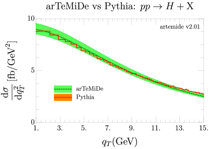
Figure 1: The cross section in eq. (4) integrated over all rapidity range with artemide2.01 at NNLO and PYTHIA. The errors of PYTHIA are included, although not clearly visible. The shaded area shows the variation band in $\tilde{\mu}$, see eq. (46).

  

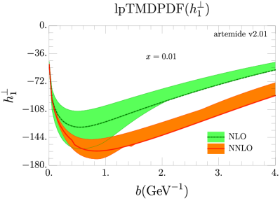
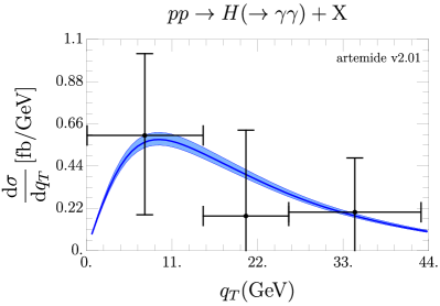
Figure 2: (left) The lpTMDPDF, eq. (17-18), as a function of $\bm{b}$ at $x=0.01$. The shaded area shows the variation band in $\tilde{\mu}$, see eq. (46). (right) Comparison of Higgs-production cross-section with variation band to the measurement presented in Khachatryan:2015rxa by CMS collaboration.

In fig. 2 (left) we have plotted lpTMDPDF, eq. (17-18), as a function of $\bm{b}$ at $x=0.01$ at NLO and at NNLO. The NNLO includes the perturbative correction to the first non-trivial order (which is NLO). This correction appears to be large, say almost a factor 2. The bands show the sensitivity of the distribution to the change of the OPE scale $\tilde{\mu}\to c_{4}\tilde{\mu}$ with $c_{4}\in(0.5,2)$, see eq. (46). The relative size of the band decreases between NLO and NNLO. Altogether, this figure points to the fact that the lpTMDPDF effects could have been underestimated up to now.

The experimental data on the Higgs differential cross section are still affected by big errors. For a demonstration we have considered the cross section in eq. (4) measured at CMS collaboration, where the rapidity is integrated in the interval indicated by that experiment Khachatryan:2015rxa . Because the experimental cross section just uses the data from one particular decay of the Higgs boson we have normalized our cross section with the experimental one integrating in the interval of transverse momenta shown in fig. 2 (right). From this figure it is clear that currently the data are not sensitive to the TMD structures.

In the Higgs production cross-section the lpTMDPDF mainly affects the low-$q_{T}$ region, as it is demonstrated in fig. 3. Practically, the lpTMDPDF can be distinguished from the unpolarized TMDPDF at $q_{T}\lesssim 5$-8GeV, where it modifies the values of cross-section by about $5\%$. Such value of variation band is typical for NNLO approximation, see e.g. Cruz-Martinez:2018rod . In fig. 3 (right) we compare the NNLO cross sections the size of the variation band, which is the maximum deviation value obtained from the variation of all three scales (in $\zeta$-prescription) by factors $c_{i}\in(0.5,2)$ Scimemi:2018xaf . The variation band is of the order of few percents and the main contribution to it is the $\mu$-band (the scale between hard part and the TMD-evolution factor). Nowadays, these factors can be pushed to N³LO reducing the variation band further, if necessary.

  

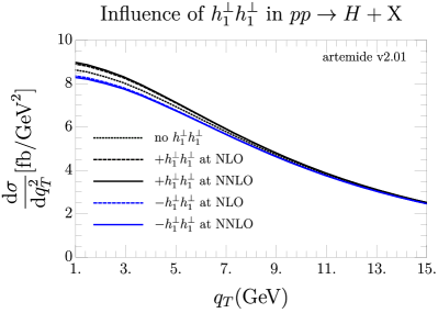
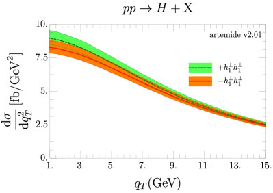
Figure 3: Cross section for Higgs production including linearly polarized gluon effects at different orders. (left) The motion of center lines of cross-section integrated over all rapidities at different perturbative orders for lpTMDPDF. The black (blue) lines correspond the case of positive (negative) contribution for $h_{1}^{\perp}h_{1}^{\perp}$-term in eq. (54). (right) The scale-variation band for the cross section at NNLO. The parity even (odd) Higgs case is represented with a green (orange) band. In both figures the center of mass energy is set as in Khachatryan:2015rxa and rapidity is integrated over its complete range.

Finally, we comment on the positivity relation formulated in ref. Mulders:2000sh :

$$|f_{1}(x,\bm{q}_{T})|-|h_{1}^{\perp}(x,\bm{q}_{T})|>0.$$ (55)

This relation is a consequence of positive definiteness of the gluon-polarization matrix in a free theory, and certainty hold at LO. However, it does not need to be accomplished at higher order in perturbation theory. The positivity bound is formulated in momentum space, whereas all perturbative calculation are performed in coordinate space. This causes an additional problem since the Hankel transform of a positive function is not necessary a positive function. Within our model we have checked that it is easy to get a violation of this bound, for any fixed value of $x$ and $q_{T}$. Typically, the violation happens in the vicinity of sign change point of $f_{1}$ (note, that our realization of $f_{1}$ is positive-definite in $\bm{b}$-space). Outside of this point the inequality in eq. (55) is respected. The situation is exemplified in fig. 4, where we plot the ratio of $|f_{1}|/|h_{1}^{\perp}|$ at different values of $q_{T}$ with fixed $x$ (left) and viceversa (right). We also note that the positions of zeros in TMDPDFs strongly depends on the non-perturbative input. In particular, selecting some appropriate model one can, possibly, remove the zero from unpolarized TMDPDF, or fix positions of zeros equal in both gluon TMDPDFs. In other words eq. (55) can be used as a serious constraint on non-perturbative part of the TMD distributions. However, we do not see enough theoretical justification for such an approach at the moment.

We have also observed that the ratio $|h_{1}^{\perp}|/|f_{1}|$ tends to saturate at smaller values of $x$ as it is suggested f.i. by McLerran:1993ka . Then for extreme small values of $x\sim 10^{-4}$ it is violated again. However, such values can be outside the applicability region of our calculation since the perturbative expressions for $f_{1}$ Echevarria:2016scs and $h_{1}^{\perp}$ (50, 51) have contributions $\sim a_{s}^{n+1}\ln^{n}(x)/x$ that should be resummed for a proper comparison.

5 Conclusions

The gluon transverse momentum dependent parton distribution function (lpTMDPDF) typically accompanies unpolarized gluon TMDPDF within a TMD factorized cross-section. A good example is the factorization formula for the Higgs-production cross-section, where these distributions enter in a plain sum. For this reason, both distributions should be considered at the same order of perturbative accuracy. We have calculated the $a_{s}^{2}$-part (NNLO) for the matching coefficient of lpTMDPDF to twist-2 collinear distributions, which is the main result of this paper. Thanks to this calculation, lpTMDPDF can be considered at the same level of theoretical accuracy as the unpolarized gluon TMDPDF Gehrmann:2014yya ; Echevarria:2016scs . The corresponding formulas are collected in sec.3.2, 3.3. They are also attached to the publication in the form of Mathematica-notebook. The module for the numerical evaluation of lpTMDPDF is added to the artemide package that can be downloaded from web .

The impact of NNLO correction for lpTMDPDF is very significant and practically doubles the value of the function for moderate $\bm{b}$. This fact should not be considered much surprising given that LO term ($a_{s}^{0}$-term) for lpTMDPDF vanishes and the correction that we provide is the one to the first non-null order. The relevance of this effect in the Higgs cross section has been discussed in sec. 4 and it is resumed in figs. 2-3. Unfortunately, at the moment we have not a reliable model for the non-perturbative part of the gluon TMD distribution, and in this work, we have adapted values for distributions extracted in refs. Scimemi:2017etj ; Bertone:2019nxa . A more detailed study on the non-perturbative part of the gluon TMDPDF is certainly worth in the future. Surprisingly, the model built by us agrees with PYTHIA prediction for low $q_{T}$ values, which are the relevant ones for TMD studies.

In several papers, it has been suggested that unpolarized and linearly polarized gluon TMDPDFs can be measured in association with heavy-quark production Mukherjee:2016cjw ; Boer:2017xpy ; Efremov:2017iwh ; Efremov:2018myn ; Kishore:2018ugo ; Echevarria:2019ynx ; Marquet:2017xwy . We leave an analysis of these processes for future work because at the moment we miss a full factorization theorem for each of these cases. Nevertheless, the consistency of data with the factorization hypothesis can always be checked with the result provided in this work.

         

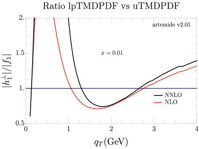
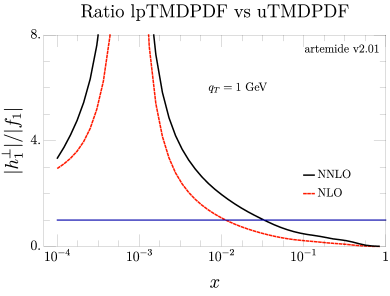
Figure 4: Ratio of linearly polarized and unpolarized gTMD to check eq. (2) as a function of $q_{T}$ at fixed $x=0.01$ (left) and as a function of $x$ at fixed $q_{T}=1$ GeV (right).

Appendix A Relevant set of master integrals for linearly polarized gluon TMD

Three different types of diagrams arise in the calculation of the unsubstracted TMDPDF matrix element for linearly polarized gluons and the can be addressed on the basis that the exchanged gluons are pure-virtual, virtual-real or real-real. The pure-virtual diagrams, are zero in the dimensional regularization due to the absence of a Lorentz-invariant scale in our scheme of calculation. The virtual-real and real-real diagrams have respectively one and two cut propagators and should be computed directly. The calculation of these two types of diagrams is analogous to the calculation made in ref. Echevarria:2015usa ; Echevarria:2016scs for the case of unpolarized TMDPDF, albeit with a different Lorentz structure. The main difference and difficulty comes from the term proportional to $b^{\mu}b^{\nu}$. The contraction of this term with the projectors generates terms in the numerator as $(\bm{bq})^{2}$ (where $\bm{q}$ is a loop-momentum), making the evaluation of the diagrams involved.

For virtual-real diagrams this difficulty can be by-passed by calculating separately virtual subdiagrams. This approach allows to contract the projector only with the real loop-momentum, simplifying the calculation of integrals. For real-real integrals no subdiagrams can be calculated. A set of master integrals in which these diagrams can be decomposed was developed in Echevarria:2016scs . In this appendix we present the decomposition of the master integrals original for this work.

A general master integral can be written as

$$F_{abcd}[R]=(2\pi)^{2}\int\frac{d^{d-1}k\,d^{d-1}l}{(2\pi)^{2d}}\frac{R\,e^{i(\bm{kb})}e^{i(\bm{lb})}\delta(k^{2})\theta(-k^{-})\delta(l^{2})\theta(-l^{-})}{[(l+p)^{2}]^{a}[(k+p)^{2}]^{b}[(k+l+p)^{2}]^{c}[(k+l)^{2}]^{d}}\ ,$$ (56)

where $R=\{1,(\bm{kb})^{2},(\bm{kb})(\bm{lb}),(\bm{lb})^{2}\}$. The bold font denotes the scalar product of transverse components only with Euclidian metric. The components $k^{+}$ and $l^{+}$ can be integrated with the help of the introduction of a delta function

$$1=\int_{-\infty}^{\infty}d\eta\,p^{+}\delta\left((1-\eta)p^{+}+l^{+}\right)$$ (57)

and they do not enter in the loop-integration (indicated by a $d-1$ integral).

The integrals with $R=1$, $F_{abcd}[1]\equiv F_{abcd}$ are presented in the Appendix C of Echevarria:2016scs . In that case, the sum of the indices $abcd$ of the integral is 2. In the present calculation, the new integrals with $R\neq 1$ and the sum of the indices $abcd$ is 3. Some of the new integrals can be expressed as a combination of older results,

$$F_{0210}[(\bm{kb})^{2}]/\bm{B}= 2\left((1+2\epsilon)(x-\eta)-\frac{\epsilon(1-2\epsilon)}{1+\epsilon}\frac{1-\eta}{x}\right)F_{0110}-\frac{2(1-2\epsilon)}{1+\epsilon}(1-x)F_{0020},$$ (58)

$$F_{0210}[(\bm{kb})(\bm{lb})]/\bm{B}= \frac{2(1-2\epsilon)}{1+\epsilon}\frac{1-\eta}{1+x-\eta}\left(\epsilon\frac{1-\eta}{x}F_{0110}-(1+\epsilon)(\eta-x)F_{0110}+(1-x)F_{0020}\right)$$

$$+2(1+x-\eta)F_{(-1)210}+2\eta F_{0110},$$ (59)

$$F_{0210}[(\bm{lb})^{2}]/\bm{B}= \frac{x}{(1+x-\eta)^{2}}\Big{(}\frac{2(1-2\epsilon)}{1+\epsilon}(x(\eta-x)-(1+\epsilon)(1-\eta))F_{0110}$$

$$+\epsilon\frac{2(1-2\epsilon)}{1+\epsilon}x(1-x)F_{0020}-2(1-2\epsilon)(1-\eta)^{2}F_{0110}\Big{)}-4(1-\eta)F_{(-1)210}$$

$$-\frac{1}{(1+x-\eta)^{2}}\left(\frac{2\epsilon(1-2\epsilon)}{1+\epsilon}\frac{(1-\eta)^{3}}{x}-2\eta(1-2\epsilon)(1-\eta)^{2}\right)F_{0110}$$

$$-\frac{2(1-2\epsilon)}{1+\epsilon}\frac{(1-\eta)^{2}}{(1+x-\eta)^{2}}(1-x)F_{0020},$$ (60)

$$F_{0120}[(\bm{kb})^{2}]/\bm{B}= \left(4(x-\eta)+\frac{2(1-2\epsilon)}{1+\epsilon}\frac{1-x}{x}(1+x-\eta)\right)F_{0020}$$

$$+\epsilon\frac{2(1-2\epsilon)}{1+\epsilon}\frac{1-\eta}{x^{2}}(1+x-\eta)F_{0110},$$ (61)

$$F_{0120}[(\bm{kb})(\bm{lb})]/\bm{B}= -\frac{2(1-2\epsilon)}{1+\epsilon}\frac{1-\eta}{x}\left(\frac{\epsilon(1-\eta)}{x}F_{0110}+(1-x)F_{0020}\right)$$

$$-2F_{0110}+2(1+x-\eta)F_{(-1)210}+2\eta F_{0020},$$ (62)

$$F_{0120}[(\bm{lb})^{2}]/\bm{B}= \frac{2(1-2\epsilon)}{1+\epsilon}\frac{(1-\eta)^{2}}{x(1+x-\eta)}\left(\epsilon\frac{1-\eta}{x}F_{0110}+(1+\epsilon)\frac{x}{1-\eta}F_{0110}+(1-x)F_{0020}\right)$$

$$-4(1-\eta)F_{(-1)210},$$ (63)

$$F_{1020}[(\bm{kb})^{2}]/\bm{B}= \frac{2(1-2\epsilon)}{1+\epsilon}\frac{(\eta-x)^{2}}{x\eta}\left(\epsilon\frac{\eta-x}{x}F_{1010}+(1+\epsilon)\frac{x}{\eta-x}F_{1010}+(1-x)F_{0020}\right)$$

$$+4(x-\eta)F_{1(-1)20},$$ (64)

$$F_{1020}[(\bm{kb})(\bm{lb})]/\bm{B}= -\frac{2(1-2\epsilon)}{1+\epsilon}\frac{\eta-x}{x}\left(\epsilon\frac{\eta-x}{x}F_{1010}+(1-x)F_{0020}\right)$$

$$-2F_{1010}+2(1+x-\eta)F_{0020}+2\eta F_{1(-1)20},$$ (65)

$$F_{1020}[(\bm{lb})^{2}]/\bm{B}= \frac{2(1-2\epsilon)}{1+\epsilon}\frac{\eta}{x}\left(\epsilon\frac{\eta-x}{x}F_{1010}+(1-x)F_{0020}\right)$$

$$-4(1-\eta)F_{0020},$$ (66)

$$F_{0021}[(\bm{kb})^{2}]/\bm{B}= -\frac{2(1-2\epsilon)}{1-\epsilon}\frac{\eta-x}{1-x}\left((1+x-\eta)F_{0020}-(\eta-x)F_{0011}\right)$$

$$+4(x-\eta)\left(F_{0011}-F_{0020}-F_{(-1)021}\right),$$ (67)

$$F_{0021}[(\bm{kb})(\bm{lb})]/\bm{B}= \frac{2(1-2\epsilon)}{1-\epsilon}\frac{(\eta-x)(1-\eta)}{1-x}\left(F_{0020}+F_{0011}\right)+2(1+x-2\eta)F_{(-1)021}$$

$$-2(1-\eta)\left(F_{0011}-F_{0020}\right)-2F_{0020},$$ (68)

$$F_{0021}[(\bm{lb})^{2}]/\bm{B}= -\frac{2(1-2\epsilon)}{1-\epsilon}\frac{1-\eta}{1-x}\left(\eta F_{0020}-(1-\eta)F_{0011}\right)-4(1-\eta)F_{(-1)021},$$ (69)

where $\mathbf{B}=\bm{b}^{2}/4$.

Additionally, we have met three integrals that could not be reduced to a combination of known results: $F_{1110}[(\bm{kb})^{2}]$, $F_{1110}[(\bm{kb})(\bm{lb})]$, $F_{1110}[(\bm{lb})^{2}]$. For these integrals we have derived the expressions in the Schwinger parameterization, and evaluated them in $\epsilon$-expansion up to the finite term following the strategy described in the book Smirnov:2004ym .

Appendix B Logarithm terms of matching coefficient for lpTMDPDF

In this appendix the logarithmic part of the matching coefficients for lpTMDPDFs are collected. Note that these coefficients are not original, in the sense that they can be predicted from the NLO matching derived in Echevarria:2015uaa ; Gutierrez-Reyes:2017glx via evolution equations as it is described in sec. 3.2. In our calculation we have derived these expressions directly, as part of the checks.

Recalling that the perturbative expansion of the coefficient function in eq. (12) is

$$\delta^{L}\!C_{g\leftarrow f}(x,\bm{b};\mu,\zeta,\mu)=\sum_{n=1}^{\infty}a_{s}^{n}\delta^{L}\!C^{[n]}_{g\leftarrow f}(x,\bm{b};\mu,\zeta,\mu),$$ (70)

with $a_{s}=g^{2}/(4\pi)^{2}$ and solving the system of eq. (40, 41) we obtain

$$\delta^{L}\!C^{[1]}_{g\leftarrow f}(x,\bm{b};\mu,\zeta,\mu) = \delta^{L}\!C^{(1,0,0)}_{g\leftarrow f}(x),$$ (71)

$$\delta^{L}\!C^{[2]}_{g\leftarrow f}(x,\bm{b};\mu,\zeta,\mu) = \left(-\frac{1}{2}\mathbf{L}_{\mu}^{2}+\mathbf{L}_{\mu}\mathbf{l}_{\zeta}\right)\delta^{L}\!C^{(2,1,1)}_{g\leftarrow f}(x)+\mathbf{L}_{\mu}\delta^{L}\!C^{(2,1,0)}_{g\leftarrow f}(x)+\delta^{L}\!C^{(2,0,0)}_{g\leftarrow f}(x),$$ (72)

where

$$\mathbf{L}_{\mu}=\ln\left(\frac{\mu^{2}\bm{b}^{2}}{4e^{-\gamma_{E}}}\right),\qquad\mathbf{l}_{\zeta}=\ln\left(\frac{\mu^{2}}{\zeta}\right).$$ (73)

Using expression for the NLO coefficients (48,49) and the LO DGLAP kernels Altarelli:1977zs and expressions for anomalous dimensions (see e.g.Echevarria:2016scs ) we obtain

$$\delta^{L}\!C^{(2,1,1)}_{g\leftarrow g}(x) = -8C^{2}_{A}\frac{1-x}{x},$$ (74)

$$\delta^{L}C_{g\leftarrow g}^{(2;1,0)}(x) = -16C_{A}^{2}\Big{\{}\frac{1+x}{x}\ln x+\frac{1-x}{x}\left[\frac{x}{6}(2-x)+\frac{15}{4}-\ln(1-x)\right]\Big{\}}$$

$$+16C_{F}T_{r}N_{f}\left[\frac{1}{3}\frac{1-x}{x}\left(2+(2-x)x\right)+\ln x\right]+\frac{16}{3}C_{A}T_{r}N_{f}\frac{1-x}{x},$$

$$\delta^{L}\!C^{(2,1,1)}_{g\leftarrow q}(x) = -8C_{F}C_{A}\frac{1-x}{x},$$ (76)

$$\delta^{L}C_{g\leftarrow q}^{(2;1,0)}(x) = -4C_{F}C_{A}\left[\frac{1-x}{x}\left(\frac{43}{3}+x\right)+4\frac{1+x}{x}\ln x\right]$$

$$+4C_{F}^{2}\left[\frac{1-x}{x}(x+4\ln(1-x))+2\ln x\right]+\frac{32}{3}C_{F}T_{r}N_{f}\frac{1-x}{x},$$

where $C_{A}=N_{c}$, $C_{F}=(N_{c}^{2}-1)/2N_{c}$ are Casimir eigenvalues of adjoint and fundamental representation for $SU(N_{c})$-gauge group, $T_{r}=1/2$ is the normalization of Gell-Mann matrices, and $N_{f}$ is the number of quark flavors.

References

- (1) J. R. Ellis, M. K. Gaillard and D. V. Nanopoulos, A Phenomenological Profile of the Higgs Boson, Nucl. Phys. B106 (1976) 292.
- (2) M. Spira, A. Djouadi, D. Graudenz and P. M. Zerwas, Higgs boson production at the LHC, Nucl. Phys. B453 (1995) 17–82, [hep-ph/9504378].
- (3) A. Djouadi, The Anatomy of electro-weak symmetry breaking. I: The Higgs boson in the standard model, Phys. Rept. 457 (2008) 1–216, [hep-ph/0503172].
- (4) S. Catani, E. D’Emilio and L. Trentadue, The Gluon Form-factor to Higher Orders: Gluon Gluon Annihilation at Small transverse, Phys. Lett. B211 (1988) 335–342.
- (5) J. Collins, Foundations of perturbative QCD. Cambridge University Press, 2013.
- (6) M. G. Echevarria, A. Idilbi and I. Scimemi, Factorization Theorem For Drell-Yan At Low And Transverse Momentum Distributions On-The-Light-Cone, JHEP 07 (2012) 002, [1111.4996].
- (7) M. G. Echevarria, A. Idilbi and I. Scimemi, Unified treatment of the QCD evolution of all (un-)polarized transverse momentum dependent functions: Collins function as a study case, Phys. Rev. D90 (2014) 014003, [1402.0869].
- (8) A. Vladimirov, Structure of rapidity divergences in soft factors, JHEP 04 (2018) 045, [1707.07606].
- (9) M. G. Echevarria, T. Kasemets, P. J. Mulders and C. Pisano, QCD evolution of (un)polarized gluon TMDPDFs and the Higgs -distribution, JHEP 07 (2015) 158, [1502.05354].
- (10) S. Catani and M. Grazzini, QCD transverse-momentum resummation in gluon fusion processes, Nucl. Phys. B845 (2011) 297–323, [1011.3918].
- (11) D. Boer, W. J. den Dunnen, C. Pisano, M. Schlegel and W. Vogelsang, Linearly Polarized Gluons and the Higgs Transverse Momentum Distribution, Phys. Rev. Lett. 108 (2012) 032002, [1109.1444].
- (12) T. Becher, M. Neubert and D. Wilhelm, Higgs-Boson Production at Small Transverse Momentum, JHEP 05 (2013) 110, [1212.2621].
- (13) P. J. Mulders and J. Rodrigues, Transverse momentum dependence in gluon distribution and fragmentation functions, Phys. Rev. D63 (2001) 094021, [hep-ph/0009343].
- (14) T. Becher and M. Neubert, Drell-Yan Production at Small , Transverse Parton Distributions and the Collinear Anomaly, Eur. Phys. J. C71 (2011) 1665, [1007.4005].
- (15) T. Gehrmann, T. Luebbert and L. L. Yang, Calculation of the transverse parton distribution functions at next-to-next-to-leading order, JHEP 06 (2014) 155, [1403.6451].
- (16) M. G. Echevarria, I. Scimemi and A. Vladimirov, Unpolarized Transverse Momentum Dependent Parton Distribution and Fragmentation Functions at next-to-next-to-leading order, JHEP 09 (2016) 004, [1604.07869].
- (17) D. Gutierrez-Reyes, I. Scimemi and A. A. Vladimirov, Twist-2 matching of transverse momentum dependent distributions, Phys. Lett. B769 (2017) 84–89, [1702.06558].
- (18) M.-X. Luo, X. Wang, X. Xu, L. L. Yang, T.-Z. Yang and H. X. Zhu, Transverse Parton Distribution and Fragmentation Functions at NNLO: the Quark Case, 1908.03831.
- (19) I. Scimemi and A. Vladimirov, Systematic analysis of double-scale evolution, JHEP 08 (2018) 003, [1803.11089].
- (20) J. Cruz-Martinez, T. Gehrmann, E. W. N. Glover and A. Huss, Second-order QCD effects in Higgs boson production through vector boson fusion, Phys. Lett. B781 (2018) 672–677, [1802.02445].
- (21) I. Scimemi and A. Vladimirov, Analysis of vector boson production within TMD factorization, Eur. Phys. J. C78 (2018) 89, [1706.01473].
- (22) V. Bertone, I. Scimemi and A. Vladimirov, Extraction of unpolarized quark transverse momentum dependent parton distributions from Drell-Yan/Z-boson production, JHEP 06 (2019) 028, [1902.08474].
- (23) X. Chen, T. Gehrmann, E. W. N. Glover, A. Huss, Y. Li, D. Neill et al., Precise QCD Description of the Higgs Boson Transverse Momentum Spectrum, Phys. Lett. B788 (2019) 425–430, [1805.00736].
- (24) M. G. Echevarria, I. Scimemi and A. Vladimirov, Transverse momentum dependent fragmentation function at next-to-next-to leading order, Phys. Rev. D93 (2016) 011502, [1509.06392].
- (25) M. G. Echevarria, I. Scimemi and A. Vladimirov, Universal transverse momentum dependent soft function at NNLO, Phys. Rev. D93 (2016) 054004, [1511.05590].
- (26) D. Gutierrez-Reyes, I. Scimemi and A. Vladimirov, Transverse momentum dependent transversely polarized distributions at next-to-next-to-leading-order, JHEP 07 (2018) 172, [1805.07243].
- (27) G. Bozzi, S. Catani, D. de Florian and M. Grazzini, Transverse-momentum resummation and the spectrum of the Higgs boson at the LHC, Nucl. Phys. B737 (2006) 73–120, [hep-ph/0508068].
- (28) S. Mantry and F. Petriello, Factorization and Resummation of Higgs Boson Differential Distributions in Soft-Collinear Effective Theory, Phys. Rev. D81 (2010) 093007, [0911.4135].
- (29) D. de Florian, G. Ferrera, M. Grazzini and D. Tommasini, Transverse-momentum resummation: Higgs boson production at the Tevatron and the LHC, JHEP 11 (2011) 064, [1109.2109].
- (30) W. Bizoń, X. Chen, A. Gehrmann-De Ridder, T. Gehrmann, N. Glover, A. Huss et al., Fiducial distributions in Higgs and Drell-Yan production at N3LL+NNLO, JHEP 12 (2018) 132, [1805.05916].
- (31) D. Boer, S. J. Brodsky, P. J. Mulders and C. Pisano, Direct Probes of Linearly Polarized Gluons inside Unpolarized Hadrons, Phys. Rev. Lett. 106 (2011) 132001, [1011.4225].
- (32) A. Metz and J. Zhou, Distribution of linearly polarized gluons inside a large nucleus, Phys. Rev. D84 (2011) 051503, [1105.1991].
- (33) F. Dominguez, J.-W. Qiu, B.-W. Xiao and F. Yuan, On the linearly polarized gluon distributions in the color dipole model, Phys. Rev. D85 (2012) 045003, [1109.6293].
- (34) C. Pisano, D. Boer, S. J. Brodsky, M. G. A. Buffing and P. J. Mulders, Linear polarization of gluons and photons in unpolarized collider experiments, JHEP 10 (2013) 024, [1307.3417].
- (35) A. Dumitru, T. Lappi and V. Skokov, Distribution of Linearly Polarized Gluons and Elliptic Azimuthal Anisotropy in Deep Inelastic Scattering Dijet Production at High Energy, Phys. Rev. Lett. 115 (2015) 252301, [1508.04438].
- (36) A. Mukherjee and S. Rajesh, Linearly polarized gluons in charmonium and bottomonium production in color octet model, Phys. Rev. D95 (2017) 034039, [1611.05974].
- (37) D. Boer, P. J. Mulders, J. Zhou and Y.-j. Zhou, Suppression of maximal linear gluon polarization in angular asymmetries, JHEP 10 (2017) 196, [1702.08195].
- (38) A. V. Efremov, N. Ya. Ivanov and O. V. Teryaev, How to measure the linear polarization of gluons in unpolarized proton using the heavy-quark pair leptoproduction, Phys. Lett. B777 (2018) 435–441, [1711.05221].
- (39) A. V. Efremov, N. Y. Ivanov and O. V. Teryaev, The ratio in heavy-quark pair leptoproduction as a probe of linearly polarized gluons in unpolarized proton, Phys. Lett. B780 (2018) 303–307, [1801.03398].
- (40) R. Kishore and A. Mukherjee, Accessing linearly polarized gluon distribution in production at the electron-ion collider, Phys. Rev. D99 (2019) 054012, [1811.07495].
- (41) M. G. Echevarria, Proper TMD factorization for quarkonia production: as a study case, 1907.06494.
- (42) C. Marquet, C. Roiesnel and P. Taels, Linearly polarized small- gluons in forward heavy-quark pair production, Phys. Rev. D97 (2018) 014004, [1710.05698].
- (43) L. D. McLerran and R. Venugopalan, Gluon distribution functions for very large nuclei at small transverse momentum, Phys. Rev. D49 (1994) 3352–3355, [hep-ph/9311205].
-
(44)
“artemide web-page, https://teorica.fis.ucm.es/artemide/
artemide repository, https://github.com/vladimirovalexey/artemide-public.” - (45) I. Scimemi, A. Tarasov and A. Vladimirov, Collinear matching for Sivers function at next-to-leading order, JHEP 05 (2019) 125, [1901.04519].
- (46) T. Gehrmann, T. Lubbert and L. L. Yang, Transverse parton distribution functions at next-to-next-to-leading order: the quark-to-quark case, Phys. Rev. Lett. 109 (2012) 242003, [1209.0682].
- (47) M. G. Echevarria, A. Idilbi and I. Scimemi, Soft and Collinear Factorization and Transverse Momentum Dependent Parton Distribution Functions, Phys. Lett. B726 (2013) 795–801, [1211.1947].
- (48) S. Moch, J. A. M. Vermaseren and A. Vogt, The Quark form-factor at higher orders, JHEP 08 (2005) 049, [hep-ph/0507039].
- (49) T. Gehrmann, E. W. N. Glover, T. Huber, N. Ikizlerli and C. Studerus, Calculation of the quark and gluon form factors to three loops in QCD, JHEP 06 (2010) 094, [1004.3653].
- (50) A. A. Vladimirov, Soft-/rapidity- anomalous dimensions correspondence, Phys. Rev. Lett. 118 (2017) 062001, [1610.05791].
- (51) Y. Li and H. X. Zhu, Bootstrapping Rapidity Anomalous Dimensions for Transverse-Momentum Resummation, Phys. Rev. Lett. 118 (2017) 022004, [1604.01404].
- (52) J. C. Collins and D. E. Soper, Back-To-Back Jets: Fourier Transform from B to K-Transverse, Nucl. Phys. B197 (1982) 446–476.
- (53) I. Scimemi and A. Vladimirov, Power corrections and renormalons in Transverse Momentum Distributions, JHEP 03 (2017) 002, [1609.06047].
- (54) M.-X. Luo, T.-Z. Yang, H. X. Zhu and Y. J. Zhu, Transverse Parton Distribution and Fragmentation Functions at NNLO: the Gluon Case, 1909.13820.
- (55) Y. Li, D. Neill and H. X. Zhu, An Exponential Regulator for Rapidity Divergences, Submitted to: Phys. Rev. D (2016) , [1604.00392].
- (56) M. A. Shifman, A. I. Vainshtein, M. B. Voloshin and V. I. Zakharov, Low-Energy Theorems for Higgs Boson Couplings to Photons, Sov. J. Nucl. Phys. 30 (1979) 711–716.
- (57) M. Kramer, E. Laenen and M. Spira, Soft gluon radiation in Higgs boson production at the LHC, Nucl. Phys. B511 (1998) 523–549, [hep-ph/9611272].
- (58) K. G. Chetyrkin, B. A. Kniehl and M. Steinhauser, Hadronic Higgs decay to order alpha-s**4, Phys. Rev. Lett. 79 (1997) 353–356, [hep-ph/9705240].
- (59) H. M. Georgi, S. L. Glashow, M. E. Machacek and D. V. Nanopoulos, Higgs Bosons from Two Gluon Annihilation in Proton Proton Collisions, Phys. Rev. Lett. 40 (1978) 692.
- (60) V. Ahrens, T. Becher, M. Neubert and L. L. Yang, Renormalization-Group Improved Prediction for Higgs Production at Hadron Colliders, Eur. Phys. J. C62 (2009) 333–353, [0809.4283].
- (61) V. Ravindran, J. Smith and W. L. van Neerven, NNLO corrections to the total cross-section for Higgs boson production in hadron hadron collisions, Nucl. Phys. B665 (2003) 325–366, [hep-ph/0302135].
- (62) C. Anastasiou, K. Melnikov and F. Petriello, Fully differential Higgs boson production and the di-photon signal through next-to-next-to-leading order, Nucl. Phys. B724 (2005) 197–246, [hep-ph/0501130].
- (63) V. Ahrens, T. Becher, M. Neubert and L. L. Yang, Origin of the Large Perturbative Corrections to Higgs Production at Hadron Colliders, Phys. Rev. D79 (2009) 033013, [0808.3008].
- (64) NNPDF collaboration, R. D. Ball et al., Parton distributions from high-precision collider data, Eur. Phys. J. C77 (2017) 663, [1706.00428].
- (65) A. Vladimirov, Pion-induced Drell-Yan processes within TMD factorization, 1907.10356.
- (66) T. Sjostrand, S. Mrenna and P. Z. Skands, PYTHIA 6.4 Physics and Manual, JHEP 05 (2006) 026, [hep-ph/0603175].
- (67) T. Sjostrand, S. Mrenna and P. Z. Skands, A Brief Introduction to PYTHIA 8.1, Comput. Phys. Commun. 178 (2008) 852–867, [0710.3820].
- (68) CMS collaboration, V. Khachatryan et al., Measurement of differential cross sections for Higgs boson production in the diphoton decay channel in pp collisions at , Eur. Phys. J. C76 (2016) 13, [1508.07819].
- (69) V. A. Smirnov, Evaluating Feynman integrals, Springer Tracts Mod. Phys. 211 (2004) 1–244.
- (70) G. Altarelli and G. Parisi, Asymptotic Freedom in Parton Language, Nucl. Phys. B126 (1977) 298–318.