High Resolution Optical Spectroscopy of Stars in the Sylgr Stellar Stream

Abstract

We observe two metal-poor main sequence stars that are members of the recently-discovered Sylgr stellar stream. We present radial velocities, stellar parameters, and abundances for 13 elements derived from high-resolution optical spectra collected using the Magellan Inamori Kyocera Echelle spectrograph. The two stars have identical compositions (within 0.13 dex or $1.2\sigma$) among all elements detected. Both stars are very metal poor ([Fe/H] $=-2.92\pm 0.06$). Neither star is highly enhanced in C ([C/Fe] $<+1.0$). Both stars are enhanced in the $\alpha$ elements Mg, Si, and Ca ([$\alpha$/Fe] $=+0.32\pm 0.06$), and ratios among Na, Al, and all Fe-group elements are typical for other stars in the halo and ultra-faint and dwarf spheroidal galaxies at this metallicity. Sr is mildly enhanced ([Sr/Fe] $=+0.22\pm 0.11$), but Ba is not enhanced ([Ba/Fe] $<-0.4$), indicating that these stars do not contain high levels of neutron-capture elements. The Li abundances match those found in metal-poor unevolved field stars and globular clusters ($\log\epsilon$(Li) $=2.05\pm 0.07$), which implies that environment is not a dominant factor in determining the Li content of metal-poor stars. The chemical compositions of these two stars cannot distinguish whether the progenitor of the Sylgr stream was a dwarf galaxy or a globular cluster. If the progenitor was a dwarf galaxy, the stream may originate from a dense region such as a nuclear star cluster. If the progenitor was a globular cluster, it would be the most metal-poor globular cluster known.

1 Introduction

The stellar halo of the Milky Way is filled with structure. Overdensities in physical, phase, and chemical space reveal a rich history of accretion. Reconstructing this history requires knowledge of the characteristics of the stellar systems and the Milky Way’s mass distribution, so it is important to identify the nature and properties of the progenitor of new structure discovered in the Milky Way halo.

Ibata et al. (2019b), hereafter referred to as I19, discovered a number of stellar streams at high Galactic latitude ($|b|>$ 20^∘) and distance $d>$ 1 kpc from the Sun. Their search relied on the second data release from the Gaia satellite to identify significant features in position, Gaia photometry, and proper motions. Cross-matching with the Sloan Digital Sky Survey (SDSS; Yanny et al. 2009) and LAMOST catalogs (Cui et al., 2012) revealed heliocentric radial velocity ($V_{r}$) and metallicity ([Fe/H]) estimates for a small subset of stars in the streams.

I19 identified 103 potential members of a stream they named Sylgr. It stretches across the northern Galactic hemisphere between $-73^{\circ}\leq\ell\leq-95^{\circ}$ and $+50^{\circ}\leq b\leq+60$^∘. They adopted a model for the Galactic potential and used an orbit integrator to derive a best-fit orbit for this stream. The SDSS provided $V_{r}$ measurements for three stars in the Sylgr stream, and these matched the predicted $V_{r}$ values at the longitude of the three stars. This match boosts confidence in the existence of the stream and confirms the membership of these three stars. Sylgr has a highly radial, prograde rotating orbit, with Galactic pericenter $2.49\pm 0.02$ kpc and apocenter $19.4\pm 0.5$ kpc. A color-magnitude diagram, constructed from Gaia broadband photometry, reveals that all of the candidate members lie near or below the main sequence turnoff point, and by construction these stars lie near a metal-poor 12.5 Gyr isochrone.

At present, there is no obvious progenitor for the Sylgr stream, but a few clues about the nature of the progenitor are available. The STREAMFINDER algorithm, which I19 used to identify the Sylgr stream, is best suited to detect thin and kinematically-cold streams that may be formed by the disruption and dissolution of globular clusters (GCs) (Malhan & Ibata, 2018; Malhan et al., 2018). The Sloan Extension for Galactic Understanding and Exploration (SEGUE) Stellar Parameter Pipeline (SSPP; Lee et al. 2008) estimated metallicities for the three stars with SDSS spectroscopy, [Fe/H] $=-$2.38, $-$2.58, and $-$3.10. These values exhibit a considerable spread, and their average is lower than that of all known GCs in the Milky Way (${\mathrm{[Fe/H]}}>-2.4$; Carretta et al., 2014). Most of the other streams discovered by I19 show minimal metallicity dispersion and higher mean metallicity among their likely members, providing the first hint that the progenitor of the Sylgr stream may not have resembled a typical GC.

Here we present high-resolution spectroscopy of two high-probability members of the Sylgr stellar stream. These spectra permit us to measure precise $V_{r}$ values, calculate stellar parameters, and derive detailed abundances for 13 elements for each star. We present the new observational material, including $V_{r}$ measurements, in Section 2. We calculate stellar parameters and metallicities in Section 3. We derive abundances of other elements and compare them with various Galactic stellar populations in Section 4. We discuss the implications of these results for the origin of the stream in Section 5 and summarize our conclusions in Section 6.

2 Observations

We observed SDSS J120220.91$-$002038.9 (hereafter J1202$-$0020) and SDSS J120825.36$+$002440.4 (hereafter J1208$+$0024) using the Magellan Inamori Kyocera Echelle (MIKE; Bernstein et al. 2003) spectrograph on the Landon Clay (Magellan II) Telescope at Las Campanas Observatory, Chile. MIKE is a double spectrograph, and the 0$\farcs$7$\times$5$\farcs$0 entrance slit and 2$\times$2 binning on the CCD yield a spectral resolving power of $R\equiv\lambda/\Delta\lambda\sim$ 41,000 on the blue spectrograph (3350 $<\lambda<$ 5000 Å) and $R\sim$ 36,000 on the red spectrograph (5000 $<\lambda<$ 8300 Å). J1202$-$0020 and J1208$+$0024 were each observed on 2019 April 11 and 12, for total integration times of 5.00 hr and 5.61 hr, respectively. Observations were made during excellent seeing conditions, $\approx$ 0$\farcs$4–0$\farcs$6. The lunar contribution to the sky background was minimal for J1202$-$0020 and non-existent for J1208$+$0024.

We use the CarPy MIKE reduction pipeline (Kelson et al., 2000; Kelson, 2003) to perform the overscan subtraction, pixel-to-pixel flat field division, image coaddition, cosmic ray removal, sky and scattered-light subtraction, rectification of the tilted slit profiles along the orders, spectrum extraction, and wavelength calibration. We use IRAF (Tody, 1993) to stitch together and continuum-normalize the spectra. Signal-to-noise ratios in the continuum range from $\sim$ 40/1 pix^-1 near 3950 Å, $\sim$ 60/1 pix^-1 near 4550 Å, $\sim$ 45/1 pix^-1 near 5200 Å, to $\sim$ 70/1 pix^-1 near 6750 Å for the final co-added spectrum of J1202$-$0020, and they are roughly 10% lower for J1208$+$0024. Figure 1 illustrates several regions of the spectra around lines of interest.

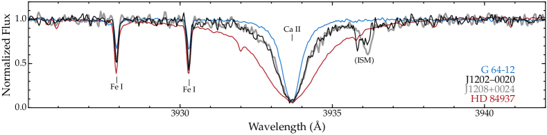
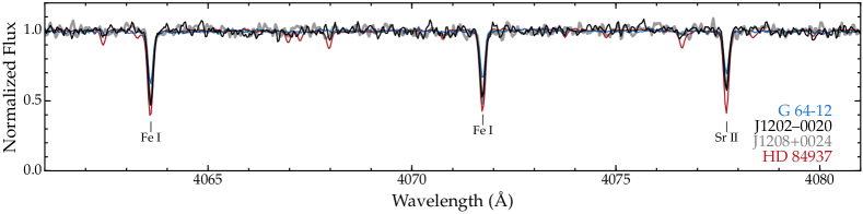
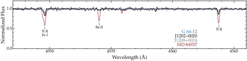
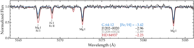
Figure 1: Selected regions of our MIKE spectra of J1202$-$0020 (thin black line) and J1208$+$0024 (bold gray line). Lines of interest are marked. Two other stars, also observed using the same MIKE setup, are shown for comparison. The spectrum of G 64-12 (catalog G 64-12) was presented in Roederer et al. (2014), and the spectrum of HD 84937 (catalog HD 84937) is described in Section 2. These two stars are only $\approx$ 200 K warmer than our target stars, and they bracket the metallicities of our target stars, as indicated in the bottom panel and demonstrated by the relative strengths of metal lines.

We measure heliocentric $V_{r}$ values by cross-correlating the echelle order containing the Mg i b triplet against a metal-poor template spectrum obtained with MIKE. We compute heliocentric velocity corrections using the IRAF “rvcorrect” task. Roederer et al. (2014) estimated uncertainties of $\approx$ 0.7 km s^-1 for $V_{r}$ measured by this method. The velocities we measure for J1202$-$0020 and J1208$+$0024, $-$203.0 km s^-1 and $-$209.5 km s^-1, respectively, compare well with the values measured from the SDSS spectra by the SSPP, $-208.56\pm 5.12$ km s^-1 and $-205.63\pm 3.28$ km s^-1, respectively. We also observed two velocity standard stars, HD 84937 (catalog HD 84937) and HD 126587 (catalog HD 126587), on these nights using the same MIKE setup. The heliocentric $V_{r}$ values we measure, $-$14.2 km s^-1 and $+$150.0 km s^-1, respectively, are in excellent agreement with previous measurements by Smith et al. (1998), Ryan et al. (1999), Carney et al. (2001, 2003), and Roederer et al. (2014). These comparisons suggest that the $V_{r}$ zeropoint of our measurements is reliable to 0.5 km s^-1 or better. We detect no significant $V_{r}$ variations in our own measurements (separated by 1 day) or between our measurements and those from the SDSS spectra (separated by 12 yr and 10 yr, respectively). Our measurements support the model for the Sylgr stream presented by I19.

3 Stellar Parameters

3.1 Effective Temperature

We calculate effective temperatures ($T_{\rm eff}$) using the metallicity-dependent color-$T_{\rm eff}$ relations presented by Casagrande et al. (2010). We first convert the SDSS $ugri$ photometry into Johnson-Cousins $BVR_{c}I_{c}$ using the transformations presented by Jordi et al. (2006). Casagrande et al. present three color-$T_{\rm eff}$ relations constructed from these bands: $B-V$, $V-R_{c}$, and $V-I_{c}$. Near-infrared Two Micron All-Sky Survey (2MASS) photometry is only available for one of the two stars, and those $JHK$ magnitudes have uncertainties in excess of 0.1 mag, so we do not make use of them. We estimate the reddening, $E(B-V)$, by two methods: the dust maps presented by Schlafly & Finkbeiner (2011), and the amount of interstellar Na i D absorption (Bohlin et al., 1978; Spitzer, 1978; Ferlet et al., 1985) as described in Roederer et al. (2018c). The reddening at these high Galactic latitudes is small in both cases, $E(B-V)\approx$ 0.022 or less. We adopt an initial model metallicity estimate of [M/H] $=-3.0\pm 0.5$ for both stars. Table 1 presents the SDSS photometry, calculated Johnson-Cousins photometry, reddening estimates, and calculated $T_{\rm eff}$ values from each of the three colors. Table 1 also presents the $T_{\rm eff}$ values we adopt, which are weighted means of the predictions from the three colors. Using the Ramírez & Meléndez (2005) color-$T_{\rm eff}$ relations, rather than those from Casagrande et al. (2010), would have yielded $T_{\rm eff}$ values higher by 74 K on average. The Alonso et al. (1999) color-$T_{\rm eff}$ relations would have yielded $T_{\rm eff}$ values cooler by 250 K on average.

Table 1: Radial Velocities, Photometry, Calculated $T_{\rm eff}$ Values, and Adopted Model Atmosphere Parameters

Star	$V_{r}$	$u$	$B$	$E(B-V)$	$T_{\rm eff}$($B-V$)	Adopted	Adopted	Adopted	Adopted
		$g$	$V$		$T_{\rm eff}$($V-R_{c}$)	$T_{\rm eff}$	log g	$v_{\rm t}$	[M/H]
		$r$	$R_{c}$		$T_{\rm eff}$($V-I_{c}$)
		$i$	$I_{c}$
	(km s-1)	(mag)	(mag)	(mag)	(K)	(K)	[cgs]	(km s-1)	(dex)
SDSS J120220.91$-$002038.9	$-$203.3 $\pm$ 0.7	18.44 $\pm$ 0.02	17.89 $\pm$ 0.02	0.020 $\pm$ 0.01	6206 $\pm$ 140	6200 $\pm$ 83	4.47 $\pm$ 0.2	1.15 $\pm$ 0.1	$-$3.0 $\pm$ 0.1
		17.56 $\pm$ 0.01	17.45 $\pm$ 0.01		6556 $\pm$ 198
		17.33 $\pm$ 0.01	17.19 $\pm$ 0.01		6092 $\pm$ 107
		17.23 $\pm$ 0.01	16.82 $\pm$ 0.01
SDSS J120825.36$+$002440.4	$-$209.5 $\pm$ 0.7	18.63 $\pm$ 0.01	18.09 $\pm$ 0.02	0.022 $\pm$ 0.01	6255 $\pm$ 142	6242 $\pm$ 84	4.46 $\pm$ 0.2	1.15 $\pm$ 0.1	$-$3.0 $\pm$ 0.1
		17.77 $\pm$ 0.01	17.67 $\pm$ 0.01		6613 $\pm$ 202
		17.55 $\pm$ 0.01	17.41 $\pm$ 0.01		6128 $\pm$ 108
		17.45 $\pm$ 0.01	17.04 $\pm$ 0.01

Note. — The $BVR_{c}I_{c}$ magnitudes are calculated from the SDSS $gri$ magnitudes using the Population II star transformations of Jordi et al. (2006).

3.2 Surface Gravity

We calculate the log of the surface gravity, log g, by interpolating 12 Gyr, $\alpha$-enhanced Yale-Yonsei ($Y^{2}$) isochrones (Demarque et al., 2004) in $T_{\rm eff}$. We assume that both stars are dwarfs on the main sequence, as suggested by the color-magnitude diagram for candidate stream members presented by I19. We estimate uncertainties in log g by varying $T_{\rm eff}$ by its uncertainty, [M/H] by $\pm 1.0$ dex, and letting the age range from 8 to 13 Gyr. These values are presented in Table 1. We also interpolate absolute magnitudes, $M_{V}$, for J1202$-$0020 and J1208$+$0024 from the $Y^{2}$ isochrones. These values, $M_{V}=5.04\pm 0.28$ and $4.95\pm 0.32$, respectively, imply distances of $3.0\pm 0.4$ kpc and $3.4\pm 0.5$ kpc.

Parallax measurements provide an alternative method of estimating the surface gravity. Unfortunately, the best parallax measurements available at present, from the second data release of the Gaia mission (Lindegren et al., 2018), are uncertain for the two stars in our sample ($\varpi=0.06\pm 0.13$ mas and $0.63\pm 0.23$ mas for J1202$-$0020 and J1208$+$0024, respectively). The I19 model orbit predicts the parallax for all stars, assuming a common distance as a function of Galactic longitude (their figure 10). The distance estimated at the longitude of these two stars is approximately $3.7\pm 0.4$ kpc, which is in agreement with distances estimated from the $Y^{2}$ isochrones.

3.3 Microturbulent Velocity and Model Metallicity

We estimate the microturbulent velocity, $v_{\rm t}$, and model metallicity, [M/H], with the help of abundances derived from Fe i and ii lines. We measure equivalent widths (EWs) using a semi-automatic routine that fits Voigt or Gaussian line profiles to continuum-normalized spectra (Roederer et al., 2014). We visually inspect each line, and we discard any line that appears blended or otherwise compromised. We examine a telluric spectrum simultaneously with the stellar spectrum, and we also discard any lines that appear to be contaminated by telluric absorption. These Fe i and ii lines are listed in Table 3.3.

Table 2: Line List

					J1202$-$0020			J1208$+$0024
Species	$\lambda$	E.P.	$\log gf$	Ref.	EW	$\log\epsilon$		EW	$\log\epsilon$
	(Å)	(eV)			(mÅ)			(mÅ)
Li i	6707.80	0.00	0.17	1	$\cdots$	2.08		$\cdots$	2.11
O i	7771.94	9.15	0.37	1	$\cdots$	$<$ 7.50		$\cdots$	$<$ 7.30
Na i	5889.95	0.00	0.11	1	89.1	3.67		85.8	3.66
Na i	5895.92	0.00	$-$0.19	1	62.7	3.54		43.5	3.26

Note. — The complete version of Table 3.3 is available in the online edition of the journal. A short version is included here to demonstrate its form and content.

References. — 1 = Kramida et al. (2018); 2 = Pehlivan Rhodin et al. (2017); 3 = Aldenius et al. (2009); 4 = Lawler & Dakin (1989), using HFS from Kurucz & Bell (1995); 5 = Wood et al. (2013); 6 = Wood et al. (2014a) for $\log gf$ values and HFS; 7 = Sobeck et al. (2007); 8 = Den Hartog et al. (2011) for both $\log gf$ values and HFS; 9 = Ruffoni et al. (2014); 10 = Belmonte et al. (2017); 11 = Lawler et al. (2015) for $\log gf$ values and HFS; 12 = Wood et al. (2014b); 13 = Roederer & Lawler (2012); 14 = Kramida et al. (2018), using HFS/IS from McWilliam (1998); 15 = Lawler et al. (2001), using HFS/IS from Ivans et al. (2006).

We make initial estimates for $v_{\rm t}$ (1.0 km s^-1) and [M/H] ($-$3.0) and interpolate one-dimensional, hydrostatic model atmospheres from the $\alpha$-enhanced ATLAS9 grid of models (Castelli & Kurucz, 2004) using an interpolation code provided by A. McWilliam (2009, private communication). We derive Fe abundances using a recent version of the line analysis software MOOG (Sneden 1973; 2017 version), which assumes local thermodynamic equilibrium (LTE).  This version of MOOG treats Rayleigh scattering, which affects the continuous opacity at shorter wavelengths, as isotropic, coherent scattering (Sobeck et al., 2011), although this update has no effect ($<$ 0.01 dex) on the abundances derived for warm stars such as these (Roederer et al., 2018c). We adopt damping constants for collisional broadening with neutral hydrogen from Barklem et al. (2000) and Barklem & Aspelund-Johansson (2005), when available, otherwise we adopt the standard Unsöld (1955) recipe. We adopt the $v_{\rm t}$ value for each model that minimizes the correlation between the abundance derived from Fe i lines and line strength. We adopt the [M/H] value for each model that approximately matches the iron (Fe, $Z=$ 26) abundance derived from Fe i lines. We iteratively determine $v_{\rm t}$ and [M/H], and the final model atmosphere parameters are reported in Table 1.

We can only measure 2 or 3 weak Fe ii lines in our spectra of J1202$-$0020 and J1208$+$0024, so we rely on Fe i lines to set [M/H].  Non-LTE corrections for a fair fraction of the Fe i lines measured in these two stars (16/43 and 15/48 lines, respectively) can be interpolated from the pre-computed grids presented in the INSPECT database by Bergemann et al. (2012b) and Lind et al. (2012). These corrections are small and consistent, with an average non-LTE correction to the LTE abundances of $+$0.04 dex ($\sigma=$ 0.01 dex). The final non-LTE metallicities for J1202$-$0020 and J1208$+$0024 are [Fe/H] $=-2.96\pm 0.09$ and $-2.89\pm 0.09$, respectively, and we adopt [M/H] $=-$3.0 for the model metallicity of each star.

3.4 Comparison with Previous Results

The SSPP fit for $T_{\rm eff}$, log g, and [Fe/H] for each of these stars: $T_{\rm eff}$ $=6452\pm 61$ K, log g $=3.77\pm 0.18$, and [Fe/H] $=-2.38\pm 0.11$ dex for J1202$-$0020; $T_{\rm eff}$ $=6502\pm 30$ K, log g $=3.60\pm 0.15$, and [Fe/H] $=-3.10\pm 0.08$ dex for J1208$+$0024. These $T_{\rm eff}$ values are warmer by about 250 K than the values we derive from color-$T_{\rm eff}$ relations. We interpolate model atmospheres with these parameters and rederive the Fe abundance from Fe i lines. The SSPP model parameters favor higher microturbulent velocities, $v_{\rm t}$ $=$ 1.5 km s^-1, and they introduce a steep correlation between the lower excitation potential (E.P.) and derived abundance, which implies that the $T_{\rm eff}$ values are too warm. The warmer SSPP $T_{\rm eff}$ value can account for about half of the [Fe/H] discrepancy for J1202$-$0020; the remaining 0.3 dex discrepancy remains unexplained. The log g values from the SSPP suggest that both stars are subgiants that have evolved beyond the main sequence turnoff. The distances implied by this more luminous evolutionary state, $d\approx 8\pm 1$ kpc, are in conflict with the distances predicted by the I19 model orbit, $d=3.7\pm 0.4$ kpc. We conclude that both stars are on the main sequence, and we adopt the stellar parameters derived in Sections 3.1–3.3.

4 Abundance Analysis

4.1 Calculations

We adopt the standard nomenclature for elemental abundances and ratios. The abundance of element X is defined as the number of X atoms per 10¹² H atoms, $\log\epsilon$(X) $\equiv\log_{10}(N_{\rm X}/N_{\rm H})+$12.0. The ratio of the abundances of elements X and Y relative to the Solar ratio is defined as [X/Y] $\equiv\log_{10}(N_{\rm X}/N_{\rm Y})-\log_{10}(N_{\rm X}/N_{\rm Y})_{\odot}$. We adopt the Solar photospheric abundances of Asplund et al. (2009). By convention, abundances or ratios denoted with the ionization state indicate the total elemental abundance derived from transitions of that particular ionization state after Saha ionization corrections have been applied.

We measure EWs for lines of other species and derive abundances using the same procedure described in Section 3. These lines are also listed in Table 3.3. We derive upper limits on the abundance when no lines of a particular element are detected. Table 3.3 lists the atomic data for all lines investigated, references for the $\log gf$ values, references for any hyperfine splitting structure (HFS) and isotope shifts (IS) used in the line component patterns for spectrum synthesis, EW measurements, abundances derived from the lines, and upper limits.

We derive abundances of lines broadened by HFS and/or IS by matching synthetic spectra, computed using MOOG, to the observed spectrum. We generate line lists for the synthetic spectra using the LINEMAKE code (C. Sneden, 2015, private communication), which is based on the line lists of Kurucz (2011) and includes many updates based on experimental laboratory data. We consider multiple isotopes in the syntheses of Li, C, N, Ba, and Eu, adopting ⁷Li/⁶Li $=$ 1000, ¹²C/¹³C $=$ 90, ¹⁴N/¹⁵N $=$ 1000, and the rapid neutron-capture process (r-process) isotopic fractions from Sneden et al. (2008) for Ba and Eu.

Table 3 lists the mean abundances, abundance ratios, and the uncertainties in these values. We estimate uncertainties in the $\log\epsilon$ abundances and [X/Fe] ratios by simultaneously resampling the stellar parameters, EWs (or approximations to the EWs in the case of lines analyzed by spectrum synthesis matching), and $\log gf$ values, and we recompute the abundances from each resample (Roederer et al., 2018b). We repeat this procedure $10^{3}$ times, and the 16th and 84th percentiles of the resulting distributions are reported as the 1$\sigma$ uncertainties in Table 3.

We detect no molecular features in the spectrum of either star. We estimate upper limits on the C and N abundances by comparing the observed spectra with synthetic spectra of the CH $G$ band near 4290–4330 Å and the CN band near 3875–3883 Å.

Numerous studies have quantitatively assessed the impact of non-LTE effects on abundances in warm, metal-poor dwarfs like the two stars analyzed here. Line-by-line non-LTE corrections to the LTE abundances are available for some species: $-$0.06 dex for Li i (Lind et al., 2009a); $-$0.12 to $-$0.28 dex for Na i (Lind et al., 2011); $+$0.04 to $+$0.08 dex for Mg i (Osorio et al., 2015; Osorio & Barklem, 2016); and $+$0.00 dex for Sr ii (Bergemann et al., 2012a). We also make approximations for a few other species. Andrievsky et al. (2008) estimated that non-LTE corrections to the abundances derived from Al i resonance lines are $\approx+$0.6 dex, and we adopt this correction. Non-LTE calculations by Bergemann et al. (2010) indicated that Cr i lines underestimate the Cr abundance by $\approx$ 0.3 to 0.4 dex, and Roederer et al. (2014) found that abundances derived from Cr i lines underestimate those derived from Cr ii lines by a similar amount. We apply a $+$0.35 dex correction to the LTE abundances derived from Cr i lines. Bergemann & Gehren (2008) found that the Mn i resonance triplet near 4030 Å underestimates abundances by several tenths of a dex. Similarly, Sneden et al. (2016) found that these lines yielded abundances lower by $\approx$ 0.3 dex relative to abundances derived from Mn ii lines and higher-excitation Mn i lines. Bergemann & Gehren (2008) attributed this discrepancy to non-LTE effects, and we apply a $+$0.3 dex correction to our LTE abundances.

Table 3: Derived Abundances

	J1202$-$0020							J1208$+$0024
Species	$\log\epsilon$	$\sigma$	[X/Fe]	[X/Fe]	$\sigma$	$N_{\rm lines}$		$\log\epsilon$	$\sigma$	[X/Fe]	[X/Fe]	$\sigma$	$N_{\rm lines}$
	LTE		LTE	Non-LTE				LTE		LTE	Non-LTE
Li i	2.08	0.09	$\cdots$	2.02	0.09	1		2.11	0.11	$\cdots$	2.08	0.11	1
C (CH)	$<$ 6.50	$\cdots$	$<+$1.03	$\cdots$	$\cdots$	$\cdots$		$<$ 6.50	$\cdots$	$<+$0.96	$\cdots$	$\cdots$	$\cdots$
N (CN)	$<$ 8.00	$\cdots$	$<+$3.13	$\cdots$	$\cdots$	$\cdots$		$<$ 8.10	$\cdots$	$<+$3.16	$\cdots$	$\cdots$	$\cdots$
O i	$<$ 7.50	$\cdots$	$<+$1.77	$\cdots$	$\cdots$	1		$<$ 7.30	$\cdots$	$<+$1.50	$\cdots$	$\cdots$	1
Na i	3.61	0.08	$+$0.33	$+$0.10	0.04	2		3.46	0.08	$+$0.11	$-$0.08	0.05	2
Mg i	4.90	0.09	$+$0.26	$+$0.33	0.06	5		4.91	0.09	$+$0.20	$+$0.27	0.07	4
Al i	3.05	0.08	$-$0.44	$+$0.16	0.05	2		2.92	0.08	$-$0.64	$-$0.04	0.06	2
Si i	4.83	0.10	$+$0.28	$\cdots$	0.07	1		4.85	0.11	$+$0.23	$\cdots$	0.07	1
Ca i	3.80	0.10	$+$0.42	$\cdots$	0.10	7		3.85	0.09	$+$0.40	$\cdots$	0.10	6
Sc ii	0.59	0.11	$+$0.40	$\cdots$	0.15	1		0.47	0.11	$+$0.21	$\cdots$	0.13	1
Ti ii	2.54	0.08	$+$0.55	$\cdots$	0.13	10		2.43	0.08	$+$0.37	$\cdots$	0.12	9
V ii	$<$ 2.30	$\cdots$	$<+$1.33	$\cdots$	$\cdots$	3		$<$ 2.30	$\cdots$	$<+$1.26	$\cdots$	$\cdots$	3
Cr i	2.62	0.11	$-$0.06	$+$0.29	0.05	3		2.54	0.10	$-$0.21	$+$0.14	0.05	3
Mn i	1.97	0.11	$-$0.50	$-$0.20	0.08	3		1.99	0.12	$-$0.55	$-$0.25	0.10	3
Fe i	4.50	0.09	$-$3.00	$-$2.96	0.09	43		4.57	0.09	$-$2.93	$-$2.89	0.09	48
Fe ii	4.70	0.14	$-$2.80	$\cdots$	0.14	2		4.68	0.14	$-$2.82	$\cdots$	0.14	3
Co i	$<$ 2.90	$\cdots$	$<+$0.87	$\cdots$	$\cdots$	2		$<$ 2.80	$\cdots$	$<+$0.70	$\cdots$	$\cdots$	2
Ni i	3.33	0.11	$+$0.07	$\cdots$	0.05	3		3.38	0.12	$+$0.05	$\cdots$	0.06	3
Zn i	$<$ 2.90	$\cdots$	$<+$1.30	$\cdots$	$\cdots$	1		$<$ 2.90	$\cdots$	$<+$1.23	$\cdots$	$\cdots$	1
Sr ii	0.16	0.10	$+$0.25	$+$0.25	0.15	2		0.18	0.10	$+$0.20	$+$0.20	0.15	2
Ba ii	$<-$1.20	$\cdots$	$<-$0.42	$\cdots$	$\cdots$	2		$<-$1.05	$\cdots$	$<-$0.34	$\cdots$	$\cdots$	2
Eu ii	$<-$0.40	$\cdots$	$<+$2.04	$\cdots$	$\cdots$	3		$<-$0.30	$\cdots$	$<+$2.07	$\cdots$	$\cdots$	3

4.2 Robust Metal Abundances

Figure 1 illustrates two key points about the metal abundances. First, spectral lines of metals including Mg, Ca, Ti, and Fe are virtually indistinguishable in J1202$-$0020 and J1208$+$0024. Given that the stellar parameters of these two stars are statistically identical, it follows that the metal abundances are also statistically identical. Secondly, the absorption line depths in these two stars are intermediate between the two comparison stars, G 64-12 (catalog G 64-12) and HD 84937 (catalog HD 84937). These stars are only slightly warmer ($6492\pm 103$ K and $6418\pm 117$ K, respectively) than J1202$-$0020 and J1208$+$0024 ($6200\pm 83$ K and $6242\pm 84$ K, respectively), and their surface gravities ($4.18\pm 0.21$ and $4.16\pm 0.14$) are only slightly lower than J1202$-$0020 and J1208$+$0024 ($4.47\pm 0.2$ and $4.46\pm 0.2$), so their spectra provide a fair comparison (Roederer et al., 2018c). It is evident from Figure 1 that the metallicity of G 64-12 (catalog G 64-12) ([Fe/H] $=-3.42\pm 0.08$) is considerably lower than that of J1202$-$0020 or J1208$+$0024. Similarly, the metallicity of HD 84937 (catalog HD 84937) ([Fe/H] $=-2.23\pm 0.07$) is considerably higher than that of J1202$-$0020 or J1208$+$0024. This comparison demonstrates that the two stars in the Sylgr stream have extremely low metallicities.

We recompute metallicities from Fe i lines under a variety of assumptions about the stellar parameters, and in all cases the [Fe/H] ratios are statistically identical. If we use a model atmosphere computed using the SSPP values (which we disfavor; see Section 3.4), then J1202$-$0020 and J1208$+$0024 have LTE metallicities of [Fe/H] $=-2.80\pm 0.09$ and $-2.74\pm 0.09$, respectively. If we use the stellar parameters inferred from a different set of transformations from $griz$ to $BVR_{C}I_{C}$ (Jester et al., 2005), which result in slightly lower temperatures and higher gravities, then J1202$-$0020 and J1208$+$0024 have LTE metallicities of [Fe/H] $=-3.07\pm 0.18$ and $-3.03\pm 0.18$, respectively. If we use model atmospheres interpolated from the MARCS grid (Gustafsson et al., 2008), instead of the ATLAS9 grid, then J1202$-$0020 and J1208$+$0024 have unchanged LTE metallicities of [Fe/H] $=-3.00\pm 0.09$ and $-2.93\pm 0.09$, respectively.

We conclude from these tests that J1202$-$0020 and J1208$+$0024 have identical metallicities, and that these metallicities are extremely low, [Fe/H] $\approx-$2.9 or so.

4.3 Lithium

Lithium (Li, $Z=$ 3) abundances have been derived previously in many unevolved metal-poor main sequence stars, which are thought to preserve the natal Li abundances. The surface convection zones are relatively shallow, so they prevent Li from being mixed to deeper layers where it can be destroyed. Early studies discovered that warm, metal-poor main sequence stars showed a near-uniform “plateau” value, $\log\epsilon$(Li) $\approx$ 2.05 (Spite & Spite, 1982; Spite et al., 1984). More recent studies that included larger samples of stars with [Fe/H] $<-$2.5 found an average decrease of a few tenths of a dex in $\log\epsilon$(Li) among the most metal-poor stars, and some also found increased abundance scatter (e.g., Ryan et al. 1999; Boesgaard et al. 2005; Aoki et al. 2009; Meléndez et al. 2010).

Figure 2 compares the Li abundances of J1202$-$0020 and J1208$+$0024 with three previous studies of Li abundances in warm, unevolved metal-poor dwarf stars in the halo field (76 unique stars), two GCs with [Fe/H] $<-$2 (59 stars in M30 (catalog M30) and 174 stars in NGC 6397 (catalog NGC 6397)), and two field stars associated with the stellar stream discovered by Helmi et al. (1999). It is clear from Figure 2 that the Li abundances in these two dwarf stars in the Sylgr stream are broadly consistent with abundances in other dwarf stars with similar metallicity in other environments.

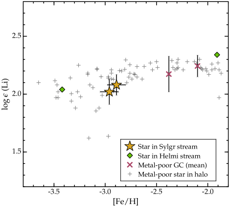
Figure 2: Comparison of $\log\epsilon$(Li) abundances in the Sylgr stream stars with those in dwarf ($T_{\rm eff}$ $>$ 5700 K; log g $>$ 3.8) stars in other metal-poor populations. The halo field star samples are drawn from Boesgaard et al. (2005), Asplund et al. (2006), Bonifacio et al. (2007, 2012), Meléndez et al. (2010), and Sbordone et al. (2010), all of whom applied non-LTE corrections to their Li abundances. Duplications have been removed. There are two GCs with [Fe/H] $<-$2 for which Li abundances have been derived in dwarf stars. The abundances for M30 (catalog M30) ([Fe/H] $=-$2.38, Cohen et al. 2011) and NGC 6397 (catalog NGC 6397) ([Fe/H] $=-$2.10, Koch & McWilliam 2011) are shown as the mean [Fe/H] ratios for each cluster and the mean $\pm$ one standard deviation for Li (Lind et al., 2009b; Gruyters et al., 2016). The Li abundances for dwarf stars in the stream discovered by Helmi et al. (1999) are quoted from Roederer et al. (2014). Li abundances have not been presented in the literature for dwarf stars in any dSph or UFD galaxy.

4.4 Carbon, Nitrogen, and Oxygen

We do not detect any atomic or molecular lines of carbon (C, $Z=$ 6), nitrogen (N, $Z=$ 7), or oxygen (O, $Z=$ 8) in either star. The upper limits derived from the non-detection of the CH G band near 4300 Å indicate that the [C/Fe] ratios are not enormously enhanced relative to the Solar ratio, but we cannot exclude [C/Fe] $<+$1.0 or so in either star. The non-detection of the CN bandhead near 3883 Å yields only uninformative upper limits on the N abundances, [N/Fe] $<+$3.2 or so. The non-detection of the O i triplet near 7770 Å also provides uninformative upper limits on the O abundances, [O/Fe] $<+$1.8 and $<+$1.5 in J1202$-$0020 and J1208$+$0024, respectively.

4.5 Sodium through Nickel

We detect lines of 11 metals from sodium (Na, $Z=$ 11) to nickel (Ni, $Z=$ 28) in the spectra of J1202$-$0020 and J1208$+$0024. Figure 3 compares the [X/Fe] ratios for each element X to the ratios found in metal-poor stars in ultra-faint dwarf (UFD) galaxies, which are low-luminosity galaxies with $M_{V}>-$7; the Ursa Minor (catalog NAME UMi Galaxy) (UMi) dwarf spheroidal (dSph) galaxy, which represents the low-luminosity ($M_{V}=-$8.8) and low-mass ($M_{*}=2.9\times 10^{5}$ $M_{\odot}$; McConnachie 2012) end of the classical dwarf galaxies; the mean abundance ratios found in metal-poor Galactic GCs; and metal-poor halo stars in the Solar neighborhood. Most of the comparison samples report abundances derived assuming LTE, so the abundance ratios in Sylgr stream stars presented in Figure 3 are the ones computed in LTE, except for Na, Mg, and Fe.

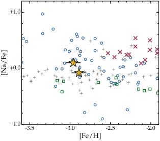
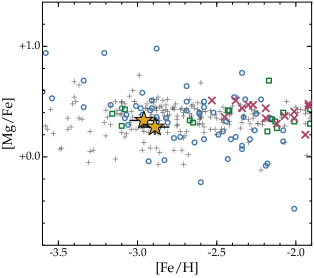
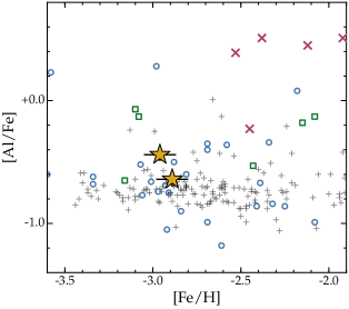
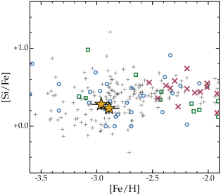
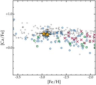
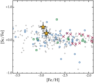
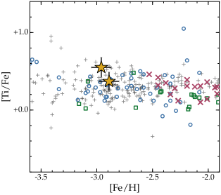
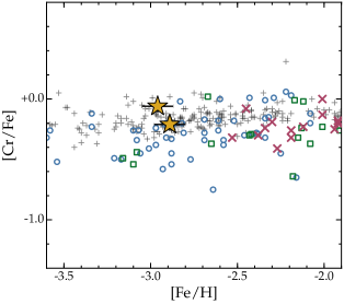
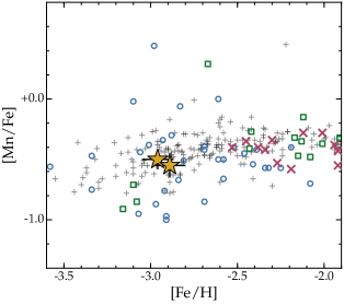
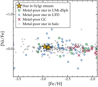
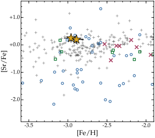
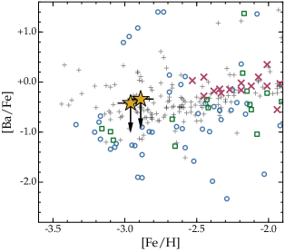
Figure 3: Comparison of abundances in Sylgr stream stars (gold stars) with abundances in stars in other stellar populations. Abundances in stars in the UMi (catalog NAME UMi Galaxy) dSph galaxy are shown by green squares. Abundances in stars in 15 UFD galaxies are shown by blue circles. The mean abundance ratios within 18 GCs are shown by red crosses. The field stars, which include dwarf and subgiant stars with $T_{\rm eff}$ $>$ 5600 K and log g $>$3.6, are shown by small gray crosses. Duplicate results have been removed. References for the comparison samples are given in Appendix A.  Note that the vertical axis on the [Sr/Fe] and [Ba/Fe] panels spans 4.4 dex, twice that of the other panels.

The two Sylgr stream stars have statistically identical abundances for all elements detected in our spectra. Quantitatively, the $\log\epsilon$ abundances ([X/Fe] ratios) differ by less than $1.2\sigma$ ($2\sigma$), and no differences exceed 0.13 dex (0.20 dex).

These two stars show an enhancement of the $\alpha$ elements magnesium (Mg, $Z=$ 12), silicon (Si, $Z=$ 14), and calcium (Ca, $Z=$ 20) relative to Fe, [$\alpha$/Fe] $\approx+0.32\pm 0.06$. This ratio is typical among stars with [Fe/H] $=-$3 in dSph and UFD galaxies and the halo, although there is considerable scatter within the dwarf galaxies. The most metal-poor GCs also exhibit a similar level of $\alpha$ enhancement.

The scandium (Sc, $Z=$ 21) and titanium (Ti, $Z=$ 22) abundances are within the range found in the comparison samples, but Figure 3 shows that they lie on the high side of the [Sc/Fe] and [Ti/Fe] distributions. Sneden et al. (2016) noticed that the abundances of Sc, Ti, and the neighboring element vanadium (V, $Z=$ 23) are often correlated in metal-poor stars. The super-Solar ratios in the two Sylgr stream stars follow the same pattern, with average [Sc/Fe] $=+0.30\pm 0.10$ and [Ti/Fe] $=+0.46\pm 0.09$. Our upper limits on the [V/Fe] ratios are, unfortunately, uninformative ([V/Fe] $<+$1.3).

Ratios among all other elements in the Fe group that we have detected in these two stars (chromium, Cr, $Z=$ 24; manganese, Mn, $Z=$ 25; and Ni) are typical. Figure 3 demonstrates that there are no distinguishing characteristics among the abundances of these elements relative to the comparison samples. Our upper limits on the cobalt (Co, $Z=$ 27) and zinc (Zn, $Z=$ 30) abundances are high and uninformative ([Co/Fe] $<+$0.7; [Zn/Fe] $<+$1.3).

4.6 Strontium and Barium

We detect the heavy element strontium (Sr, $Z=$ 38) in the spectra of both J1202$-$0020 and J1208$+$0024. The average ratio, $\mathrm{[Sr/Fe]}=+0.22\pm 0.11$, is mildly super-Solar. We do not detect barium (Ba, $Z=$ 56) in either star. We place meaningful upper limits on the Ba abundance ratios, [Ba/Fe] $<-$0.42 in J1202$-$0020 and [Ba/Fe] $<-$0.34 in J1208$+$0024, demonstrating that Ba is not enhanced in these stars.

5 Discussion

GCs and dwarf galaxies experience very different star formation histories that affect the chemical compositions of their stars. Most GCs are chemically homogeneous except for a few light elements. Stars in dwarf galaxies, on the other hand, exhibit a wide range of metallicities and ratios among their metals. A quick scan of figures 2 and 4 of Ji et al. (2019), for example, reveals that it is rare—but not unprecedented—for two randomly-selected stars within a given UFD galaxy to have the same composition. We explore in this section how the chemistry of the two Sylgr stream stars compares to that of metal-poor field stars and surviving GCs, UFD galaxies, and dSph galaxies. These ratios set empirical constraints on the yields of early supernovae in the progenitor of the Sylgr stream. We also provide order-of-magnitude limits on the density and mass of the progenitor system, and we discuss the implications of our results.

5.1 [Fe/H]

J1202$-$0020 was targeted by the SEGUE-1 survey because its colors were consistent with being an F turnoff star. The number of such candidates available in a given SEGUE field far exceeded the number of available fibers, and objects in this class were preferentially selected to be bluer—which served as a proxy for low metallicity—and brighter (Yanny et al., 2009). J1208$+$0024 has virtually identical colors, and it was selected as a quality assurance star in SEGUE-2.  We selected these stars for observation based on the availability of $V_{r}$ measurements from SEGUE to confirm their membership in the Sylgr stream. If other, more metal-rich candidate members of the Sylgr stream had not been selected for SEGUE spectroscopy based on their redder colors, then our sample could be biased toward lower-metallicity stars. We thus exercise caution while using the metallicities of these two stars to infer the metallicity distribution function (MDF) as a characteristic of the nature of the progenitor system.

The mass-metallicity relation for dwarf galaxies in the Local Group (e.g., Kirby et al. 2013) predicts that a progenitor system with a mean ${\mathrm{[Fe/H]}}\approx-2.9$ should have had an extremely low stellar mass, $M_{*}<10^{2}$ $M_{\odot}$. This mass is lower than the mass of the stars already identified by I19 as candidate members of the Sylgr stream. The actual progenitor mass is likely to be significantly larger than this estimate. In fact, no known dwarf galaxy has mean ${\mathrm{[Fe/H]}}$ below $-2.7$, which makes the extrapolated value of the mass very uncertain.

While our sample may underestimate the mean metallicity of the progenitor system, as discussed above, we can still estimate the probability of having drawn these two stars from the MDF of a progenitor like one of the surviving dSph or UFD galaxies. Figure 4 shows the empirical MDFs for the five dSph galaxies with $M_{*}<10^{6}$ $M_{\odot}$ (CVn I (catalog NAME CVn I dSph), Dra (catalog NAME Dra dSph), Leo II (catalog NAME Leo II dSph), Sex (catalog NAME Sextans Dwarf Galaxy), and UMi (catalog NAME UMi Galaxy)) from Kirby et al. (2010). The probability of randomly selecting two stars with ${\mathrm{[Fe/H]}}=-2.96$ and $-2.89$ is below 0.16%. To approximate the MDF of UFD galaxies, we compile all 72 stars observed with high spectral resolution in the 15 UFD galaxies referenced in Appendix A. The probability of randomly selecting our two stars from this UFD sample is about 12%. Therefore, it is significantly more likely that the two stars could be chosen randomly from a UFD galaxy than from a classical dSph galaxy.

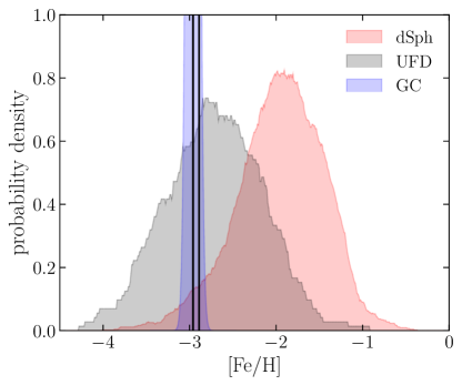
Figure 4: MDF for the sample of 1083 stars in the five smallest dSph galaxies from Kirby et al. (2010) and the 72 stars from UFD galaxies described in Figure 3. The inferred metallicities of the two Sylgr stars are shown by the vertical solid lines. The blue shaded histogram shows a Gaussian distribution, centered on J1202$-$0020, with a standard deviation of 0.05 dex typical for GCs.

These probabilities do not include the more puzzling result that the inferred metallicities of the two stars are very close. We estimate $\Delta{\mathrm{[Fe/H]}}\approx 0.07$ dex, based on the most accurate non-LTE abundance determination (Table 3). The probability of randomly selecting the first star from the UFD MDF and then selecting the second star with metallicity within $\Delta{\mathrm{[Fe/H]}}$ is only 3.1% (and much less for the dSph MDF). This conditional probability is low because the MDFs of dwarf galaxies have significant intrinsic width (about 0.5 dex) and two random stars are unlikely to have such close [Fe/H] values.

In contrast, the MDF of GCs is very narrow, with typical standard deviation below 0.05 dex, and often below observational errors (e.g., Carretta et al. 2009a). The two stars would naturally have similar values of ${\mathrm{[Fe/H]}}$ if they belonged to a now-disrupted GC.  However, such an origin of the Sylgr stream presents additional puzzles, which we discuss in Section 5.7 below.

5.2 Lithium

The Li abundance in the Sylgr stream stars, $\log\epsilon=2.05\pm 0.07$, is slightly lower than the mean Li abundances in the two GCs where Li abundances in dwarf stars have been studied, M30 (catalog M30) ($\log\epsilon=$ 2.17, $\sigma=0.16$ dex; Gruyters et al. 2016) and NGC 6397 (catalog NGC 6397) ($\log\epsilon=$ 2.24, $\sigma=0.09$ dex; Lind et al. 2009b). The probabilities of drawing the Li abundances in both Sylgr stream stars from either the M30 (catalog M30) or NGC 6397 (catalog NGC 6397) Li distributions are $\approx$ 4.3% and 0.10%, respectively. These results are sensitive to the methods of deriving $T_{\rm eff}$; Charbonnel & Primas (2005), for example, note that $\log\epsilon$(Li) will change by $\pm 0.05$ dex in response to changes of $\pm 70$ K in $T_{\rm eff}$. $T_{\rm eff}$ zeropoints can easily vary by $\pm 100$ K from one scale to another (cf. Section 3.1), and a reduction in the GC stars’ $T_{\rm eff}$ by 100 K would increase the probabilities to 10% for M30 (catalog M30) and 0.70% for NGC 6397 (catalog NGC 6397). We conclude that the Li abundances of the Sylgr stream stars are not significantly different from those of the GC stars.

No Li detections have been made in any dwarf stars in dSph or UFD galaxies, because these systems are located at large distances and their dwarf stars are faint. Li abundances ($\log\epsilon=$ 2.19, $\sigma=0.14$ dex; Monaco et al. 2010) in dwarf stars in the metal-poor ([Fe/H] $\approx-1.75$) populations of the GC $\omega$ Cen (catalog NGC 5139), which may be the nuclear remnant of a dwarf galaxy (e.g., Bekki & Freeman 2003; Ibata et al. 2019a), are also similar to the GC and field star populations.

Li has been studied previously in dwarf stars in only one metal-poor stellar stream. Roederer et al. (2010) presented Li abundances for two dwarf stars that are probable members of the stream discovered by Helmi et al. (1999), which was likely formed by a dwarf galaxy with stellar mass $\sim 10^{8}$ $M_{\odot}$ that was accreted by the Milky Way $\sim$ 5–8 Gyr ago (Koppelman et al., 2019). These results are shown in Figure 2, and they are also consistent with the Li abundances in other field stars.

Environment may not be a dominant factor in determining the Li content of metal-poor stars. The $\omega$ Cen (catalog NGC 5139), Helmi stream, and Sylgr stream results suggest that the primordial Li abundances in the progenitor systems were not remarkably different from those in the progenitors of other systems whose stars were dispersed to form the nearby stellar halo. Furthermore, Boesgaard et al. (2005) and Aoki et al. (2009) found no significant correlation between orbital properties and Li abundances in metal-poor dwarfs. It will be important in future work to assess the distribution of Li abundances in larger samples of dwarf stars in Sylgr and other nearby stellar streams. These streams both serve as proxies for more distant, surviving systems, and they offer a new opportunity to study the role of environment in Li production and depletion in the early Universe.

5.3 $\alpha$ Elements and Fe-Group Elements

The Sylgr stream stars are $\alpha$ enhanced, with an average enhancement of [$\alpha$/Fe] $\approx+0.32\pm 0.06$ among Mg, Si, and Ca. This result is typical for GCs and the most metal-poor stars in UFD and dSph galaxies. The ratios among Fe-group elements (Sc, Ti, Cr, Mn, and Ni) are also typical for stars in UFD and dSph galaxies and GCs.

The fact that both stars share ratios typical for other populations implies that ejecta from multiple progenitor supernovae are present. These abundance ratios reflect the mass-averaged supernova yields, rather than more extreme ratios that result from stochastically sampling the high-mass end of the initial mass function. The enhanced [$\alpha$/Fe] ratios indicate that the stars formed from gas enriched by the ejecta of Type II supernovae, with minimal contributions from Type Ia supernovae, so they probably formed shortly after star formation commenced. The abundance ratios do not directly reveal the stellar ages, but they suggest that the stars likely formed in an environment with a relatively high star formation rate and short chemical enrichment timescale.

5.4 Neutron-Capture Elements

The Sr abundance ([Sr/Fe] $=+0.22\pm 0.11$) and Ba upper limit ([Ba/Fe] $<-0.4$) in J1202$-$0020 and J1208$+$0024 indicate that these two stars are not highly enhanced in elements produced by neutron-capture reactions. The low Ba indicates that neither star contains metals from a low- or intermediate-mass ($\lesssim$ 5 $M_{\odot}$) companion star that passed through the asymptotic giant branch phase of evolution. Most stars with [Fe/H] $\approx-3$ do not show evidence of such enrichment (e.g., Jacobson et al. 2015), so the stars are typical in this regard. Otherwise, with such limited information it is not possible to determine what kind of nucleosynthesis process produced the Sr in these stars.

Figure 3 shows that the [Sr/Fe] ratios in the Sylgr stream stars lie in the high part of the distribution of stars in UFD galaxies. Most [Sr/Fe] ratios in UFD galaxies are $<-$1. Two notable exceptions include Ret II (catalog NAME Reticulum II) ([Sr/Fe] $=+$0.24; Ji et al. 2016b), and Tuc III (catalog NAME Tucana III) ([Sr/Fe] $=-$0.11; Hansen et al. 2017; Marshall et al. 2018), which are known to be r-process-enhanced galaxies. These two galaxies are also enhanced to varying degrees in other heavy elements produced by the r-process, like Ba ([Ba/Fe] $=+$1.04 and $-$0.03, respectively). If the Sylgr stream stars are also r-process enhanced, their level of enhancement is considerably lower than either of Ret II (catalog NAME Reticulum II) or Tuc III (catalog NAME Tucana III). We do not detect the r-process element europium (Eu, $Z=$ 63) in either spectrum, and the upper limits we derive ([Eu/Fe] $<+$2.04) are uninformative. The only other Sr-enhanced star known in a UFD galaxy is in CVn II (catalog NAME CVn II dSph) ([Sr/Fe] $=+$1.32; François et al. 2016), which has one of the highest [Sr/Ba] ratios known ($+$2.6; François et al. 2016). [Sr/Fe] ratios lower than the Sylgr stream stars are found in 11/12 (92%) of the non-r-process-enhanced UFD galaxies studied at present.

Stars with [Fe/H] $\sim-$3 in some dSph galaxies like Sextans (catalog NAME Sextans Dwarf Galaxy) and Ursa Minor (catalog NAME UMi Galaxy) show [Sr/Fe] $\sim$ 0 and [Ba/Fe] $\sim-$1 (Cohen & Huang, 2010; Tafelmeyer et al., 2010; Kirby & Cohen, 2012), potentially similar to the two stars observed in the Sylgr stream. In other dSph galaxies, like Carina (catalog NAME Carina dSph) or Draco (catalog NAME Dra dSph), [Sr/Fe] and [Ba/Fe] are both significantly sub-Solar (Cohen & Huang, 2009; Venn et al., 2012), sometimes by several dex (Fulbright et al., 2004).

Sr is not often studied in GCs. Figure 3 shows that 5/7 (71%) of the metal-poor GCs ([Fe/H] $<-1.8$) show mean [Sr/Fe] ratios $<0$, lower than the Sylgr stream stars. Ba is studied more frequently than Sr in GCs, and 14/16 (88%) of the GCs have [Ba/Fe] ratios higher than the [Ba/Fe] upper limits we have derived. Thus the enhanced [Sr/Ba] ratio we derive for the Sylgr stream, $>+0.6$, is unprecedented in metal-poor GCs.

In conclusion, the [Sr/Fe], [Ba/Fe], and [Sr/Ba] ratios found in the Sylgr stream stars are rare among stars in UFD galaxies, sometimes found among the most metal-poor stars in dSph galaxies, and not found in metal-poor GCs.

5.5 Light Elements Whose Abundances Vary in GCs

Particular abundance variations among some light elements are a sign of GC populations. Star-to-star scatter exists among the O, Na, and aluminum (Al, $Z=$ 13) abundances in stars in GCs, with the lowest [Na/Fe] and [Al/Fe] ratios coincident with those in field stars and the highest [Na/Fe] and [Al/Fe] ratios enhanced by a dex or more. Neither ratio is significantly enhanced in J1202$-$0020 or J1208$+$0024. The typical [O/Fe] ratios found in metal-poor GC stars are $\leq+0.8$ or so (e.g., Carretta et al. 2009b), considerably lower than the upper limits we derive ([O/Fe] $<+1.5$). The [Mg/Fe] ratios in some stars in a few GCs are depleted, but the [Mg/Fe] ratios in J1202$-$0020 and J1208$+$0024 do not show evidence of such depletion. These ratios are all consistent with those found in typical metal-poor field stars and so-called “first-generation” stars in GCs, and they do not exclude the possibility that the progenitor was a GC.

5.6 Other Constraints on the Nature of the Progenitor

Many GCs and UFD galaxies have velocity dispersions $\sim 5$ km s^-1 (e.g., Harris 1996; Simon & Geha 2007). The small $V_{r}$ difference between J1202$-$0020 and J1208$+$0024 ($6.5\pm 0.5$ km s^-1) cannot distinguish between GC and UFD galaxy populations, especially in an extended stellar stream whose members are not in dynamical equilibrium.

I19 note that the Sylgr stream has similar energy and angular momentum to the GCs M10 (catalog M10) (NGC 6254) and M12 (catalog M12) (NGC 6218). Neither cluster has an obvious excess of extra-tidal stars (de Boer et al., 2019; Kundu et al., 2019). I19 excluded these GCs as the progenitor based on their less radial orbits with smaller apocenters ($<5$ kpc; Baumgardt et al., 2019) and the much higher metallicities of M10 (catalog M10) and M12 (catalog M12) (${\mathrm{[Fe/H]}}\approx-1.6$ and $-1.3$; Carretta et al. 2009a) relative to the SSPP metallicity estimates. We reaffirm this conclusion on the basis of the low metallicities derived from our high-resolution spectra.

I19 identified the Sylgr stream as a long arc, suggesting that the disruption took place no more than a few orbital periods ago. The orbit reconstruction by I19 suggests a bound orbit for the Sylgr stream, with pericenter near 2.5 kpc from the Galactic center and apocenter near 20 kpc. Such an orbit has a relatively short period $\lesssim 0.5$ Gyr and can be reliably calculated, as the gravitational potential of the Galaxy is likely to be stable over many orbital periods. This is a typical prograde orbit shared by many surviving GCs.  In contrast, the pericenter of this orbit is much smaller than typical pericenters for UFD galaxies (20–40 kpc; Fritz et al. 2018; Simon 2018). Therefore, the progenitor experienced significantly stronger tidal forces than the current population of UFD galaxies, so it would have needed to be more dense than the UFD galaxies to avoid an early disruption.

The average density of Galactic material at $r=2.5$ kpc from the center is $\sim 1$ $M_{\odot}$ pc^-3. An object would remain gravitationally bound for several orbital periods if its average density exceeds roughly twice this value. GCs with orbital pericenters $\approx$2–3 kpc (Gaia Collaboration et al., 2018) have stellar densities at their half-mass radii $\approx$ 10–500 $M_{\odot}$ pc^-3, with a median value $\approx$ 100 $M_{\odot}$ pc^-3 (Baumgardt & Hilker, 2018), so they easily meet this condition. Surviving UFD galaxies have average densities $\ll 1$ $M_{\odot}$ pc^-3 within their core radii (Simon & Geha, 2007), so any UFD-like systems on orbits like that of the Sylgr stream would have disrupted long ago (cf. Roederer et al. 2018a). We conclude that the progenitor must have been substantially more dense than the surviving population of UFD galaxies.

We can estimate the minimum mass of the progenitor required to withstand the tidal forces along its orbit. If the Sylgr progenitor had a half-mass radius of $\approx$ 6 pc, similar to the surviving GCs with comparable orbital pericenters, then it would need to have had a minimum mass of $\sim 10^{3}$ $M_{\odot}$ before disruption. The initial mass of the cluster on such an orbit was likely up to a factor of 10 higher (Baumgardt et al., 2019). This order-of-magnitude estimate shows that the progenitor could contain enough stars to explain all stream candidates and persist for many orbital periods.

5.7 Implications If the Progenitor Was a GC

If the progenitor of the Sylgr stream was indeed a GC, it would be an exciting discovery. The [Fe/H] ratios of the two observed stars are considerably lower than those of the lowest-metallicity Galactic GCs, which have [Fe/H] $\approx-$2.4 (e.g., Harris, 1996). Beasley et al. (2019) considered GC systems of external galaxies that span 6 orders of magnitude in stellar mass and concluded that the MDFs of these systems have a plausible “metallicity floor” at ${\mathrm{[Fe/H]}}\approx-2.5$. Few known GCs show metallicity below that value (Forbes et al., 2018). The two stars observed in the Sylgr stream have Fe abundances that are a factor of $\approx 2.5$ lower than this floor. Although the [Fe/H] scales may systematically differ by about 0.1 dex (e.g., Carretta et al., 2009a), the metallicity of the two Sylgr stream stars is demonstrably lower than that of all known GCs.

The mass-metallicity relation for galaxies is observed to hold with only mild evolution even at high redshift (e.g., Maiolino & Mannucci, 2019). Thus the presence of a metallicity floor indicates that surviving GCs could not have formed in galaxies below a certain mass. That minimum mass is estimated to be around halo mass $M_{\rm h}\sim 10^{9}$$M_{\odot}$ (Choksi et al., 2018) or stellar mass $M_{*}\sim 10^{6}$$M_{\odot}$ (Kruijssen, 2019). The exact values are very sensitive to the unknown extrapolation of the galactic mass-metallicity relation at $z>4$, when the most metal-poor GCs are expected to form (e.g., Muratov & Gnedin, 2010; Li & Gnedin, 2014; Choksi & Gnedin, 2019).

Confirming the origin of the Sylgr stream progenitor as a GC would have significant implications for the universality of such a floor. It would indicate that GCs can form in lower-mass galaxies than had been expected previously, which is an important constraint for models of GC formation. It would also imply that a non-zero fraction of halo stars with [Fe/H] $<-$2.5 formed in GCs, rather than in situ or in UFD or dSph galaxies.

Even if the Sylgr progenitor was instead a UFD or dSph galaxy, the arguments in Section 5.6 indicate that the observed thin stream is likely a remnant of its densest part. This dense part could be a nuclear star cluster, with a stellar density similar to that of massive GCs.

6 Conclusions

We have obtained high-resolution optical spectra of two warm, main sequence stars proposed by I19 as members of the Sylgr stellar stream. We confirm previous $V_{r}$ measurements, verifying their status as members. We have derived abundances of 13 elements in each star, and we show that these two stars are chemically homogeneous at a level of $\leq 0.13$ dex. Both stars are metal-poor, with average [Fe/H] $=-2.92\pm 0.06$. The Li abundances, $\log\epsilon$(Li) $=2.05\pm 0.07$, are consistent with other unevolved stars at this metallicity. Neither star is C enhanced, with [C/Fe] $<+1.0$. Both stars are $\alpha$ enhanced, with average [$\alpha$/Fe] $\approx+0.32\pm 0.06$ among the $\alpha$ elements Mg, Si, and Ca. The ratios among other elements (Na, Al, Sc, Ti, Cr, Mn, and Ni) are typical for stars at this metallicity. Sr is mildly enhanced, with average [Sr/Fe] $=+0.22\pm 0.11$, but Ba is not, with [Ba/Fe] $<-0.4$.

We compare the chemical composition of these two stars with that of other metal-poor stars in the field and in surviving stellar systems around the Milky Way. Our results indicate that the progenitor of the Sylgr stream could have been similar to a GC or a low-mass UFD or dSph galaxy. In either case, however, some abundances are unlike those found in surviving GCs and UFD and dSph galaxies. For example, the high [Sr/Ba] ratio is not found in GC populations. On the other hand, the fact that both stars have identical metal abundances favors a GC origin. If the progenitor was a GC, it would qualify as the most metal-poor GC known, by about 0.4 dex. Dynamical considerations from the orbit of the Sylgr stream also favor a system with a relatively high stellar density, like a GC or a dense region of a UFD or dSph galaxy.

With only two stars in our sample, these considerations remain unconfirmed. Spectroscopic observations of more stars in the Sylgr stream are needed to conclusively determine its origin. If more stars are found to have nearly the same metallicity, it would very likely confirm a GC origin. Similarly, if other stream stars have different metallicities but a substantial fraction show indistinguishable values of ${\mathrm{[Fe/H]}}\approx-3$, then the latter subset of stars would still point to a disrupted GC or nuclear star cluster. Such a discovery would challenge the apparent metallicity floor of GCs and present an exciting puzzle for the theories of GC formation.

Appendix A References for Literature Data

The abundance data for the comparison samples of stars presented in Figure 3 have been compiled from many sources. Abundances in stars in the UMi (catalog NAME UMi Galaxy) dSph galaxy are taken from Shetrone et al. (2001), Sadakane et al. (2004), Cohen & Huang (2010), Kirby & Cohen (2012), and Ural et al. (2015). Abundances in stars in the UFD galaxies Boo I (catalog NAME Bootes Dwarf Spheroidal Galaxy), Boo II (catalog NAME Bootes II), Com (catalog NAME Coma Dwarf Galaxy), CVn II (catalog NAME CVn II dSph), Gru I (catalog NAME Grus I), Her (catalog NAME Her Dwarf Galaxy), Hor I (catalog NAME Hor I), Leo IV (catalog NAME Leo IV Dwarf Galaxy), Ret II (catalog NAME Reticulum II), Seg 1 (catalog NAME Segue 1), Seg 2 (catalog NAME Segue 2), Tri II (catalog NAME Tri II), Tuc II (catalog NAME Tucana II), Tuc III (catalog NAME Tucana III), and UMa II (catalog NAME UMa II Galaxy) are taken from Koch et al. (2008, 2013), Feltzing et al. (2009), Frebel et al. (2010, 2014, 2016), Norris et al. (2010a, b), Simon et al. (2010), Gilmore et al. (2013), Ishigaki et al. (2014), Koch & Rich (2014), Roederer & Kirby (2014), François et al. (2016), Ji et al. (2016a, b, c, 2019), Roederer et al. (2016b), Hansen et al. (2017), Chiti et al. (2018), Nagasawa et al. (2018), and Marshall et al. (2018). The mean abundance ratios within GCs including M15 (catalog M15), M30 (catalog M30), M53 (catalog M53), M55 (catalog M55), M68 (catalog M68), M92 (catalog M92), NGC 2419 (catalog NGC 2419), NGC 4372 (catalog NGC 4372), NGC 4833 (catalog NGC 4833), NGC 5053 (catalog NGC 5053), NGC 5694 (catalog NGC 5694), NGC 5824 (catalog NGC 5824), NGC 5897 (catalog NGC 5897), NGC 6287 (catalog NGC 6287), NGC 6397 (catalog NGC 6397), NGC 6426 (catalog NGC 6426), NGC 6535 (catalog NGC 6535), and Ter 8 (catalog Cl Terzan 8), are computed from data presented in Shetrone et al. (2001), Lee & Carney (2002), Cohen (2011), Cohen et al. (2011), Koch & McWilliam (2011, 2014), Sobeck et al. (2011), Venn et al. (2012), Mucciarelli et al. (2013), Carretta et al. (2014), Boberg et al. (2015, 2016), Roederer & Thompson (2015), San Roman et al. (2015), Schaeuble et al. (2015), Roederer et al. (2016a), Bragaglia et al. (2017), Hanke et al. (2017), and Rain et al. (2019). The field star sample (small gray crosses) includes stars with $T_{\rm eff}$ $>$ 5600 K and log g $>$3.6 from Lai et al. (2008), Bonifacio et al. (2009), Yong et al. (2013), and the main sequence and subgiant stars analyzed by Roederer et al. (2014). Duplicate results have been removed.

References

- Aldenius et al. (2009) Aldenius, M., Lundberg, H., & Blackwell-Whitehead, R. 2009, A&A, 502, 989, doi: 10.1051/0004-6361/200911844
- Alonso et al. (1999) Alonso, A., Arribas, S., & Martínez-Roger, C. 1999, A&AS, 140, 261, doi: 10.1051/aas:1999521
- Andrievsky et al. (2008) Andrievsky, S. M., Spite, M., Korotin, S. A., et al. 2008, A&A, 481, 481, doi: 10.1051/0004-6361:20078837
- Aoki et al. (2009) Aoki, W., Barklem, P. S., Beers, T. C., et al. 2009, ApJ, 698, 1803, doi: 10.1088/0004-637X/698/2/1803
- Asplund et al. (2009) Asplund, M., Grevesse, N., Sauval, A. J., & Scott, P. 2009, ARA&A, 47, 481, doi: 10.1146/annurev.astro.46.060407.145222
- Asplund et al. (2006) Asplund, M., Lambert, D. L., Nissen, P. E., Primas, F., & Smith, V. V. 2006, ApJ, 644, 229, doi: 10.1086/503538
- Barklem & Aspelund-Johansson (2005) Barklem, P. S., & Aspelund-Johansson, J. 2005, A&A, 435, 373, doi: 10.1051/0004-6361:20042469
- Barklem et al. (2000) Barklem, P. S., Piskunov, N., & O’Mara, B. J. 2000, A&A, 355, L5
- Baumgardt & Hilker (2018) Baumgardt, H., & Hilker, M. 2018, MNRAS, 478, 1520, doi: 10.1093/mnras/sty1057
- Baumgardt et al. (2019) Baumgardt, H., Hilker, M., Sollima, A., & Bellini, A. 2019, MNRAS, 482, 5138, doi: 10.1093/mnras/sty2997
- Beasley et al. (2019) Beasley, M. A., Leaman, R., Gallart, C., et al. 2019, MNRAS, 487, 1986, doi: 10.1093/mnras/stz1349
- Bekki & Freeman (2003) Bekki, K., & Freeman, K. C. 2003, MNRAS, 346, L11, doi: 10.1046/j.1365-2966.2003.07275.x
- Belmonte et al. (2017) Belmonte, M. T., Pickering, J. C., Ruffoni, M. P., et al. 2017, ApJ, 848, 125, doi: 10.3847/1538-4357/aa8cd3
- Bergemann & Gehren (2008) Bergemann, M., & Gehren, T. 2008, A&A, 492, 823, doi: 10.1051/0004-6361:200810098
- Bergemann et al. (2012a) Bergemann, M., Hansen, C. J., Bautista, M., & Ruchti, G. 2012a, A&A, 546, A90, doi: 10.1051/0004-6361/201219406
- Bergemann et al. (2012b) Bergemann, M., Lind, K., Collet, R., Magic, Z., & Asplund, M. 2012b, MNRAS, 427, 27, doi: 10.1111/j.1365-2966.2012.21687.x
- Bergemann et al. (2010) Bergemann, M., Pickering, J. C., & Gehren, T. 2010, MNRAS, 401, 1334, doi: 10.1111/j.1365-2966.2009.15736.x
- Bernstein et al. (2003) Bernstein, R., Shectman, S. A., Gunnels, S. M., Mochnacki, S., & Athey, A. E. 2003, in Proc. SPIE, Vol. 4841, Instrument Design and Performance for Optical/Infrared Ground-based Telescopes, ed. M. Iye & A. F. M. Moorwood, 1694–1704
- Boberg et al. (2015) Boberg, O. M., Friel, E. D., & Vesperini, E. 2015, ApJ, 804, 109, doi: 10.1088/0004-637X/804/2/109
- Boberg et al. (2016) —. 2016, ApJ, 824, 5, doi: 10.3847/0004-637X/824/1/5
- Boesgaard et al. (2005) Boesgaard, A. M., Stephens, A., & Deliyannis, C. P. 2005, ApJ, 633, 398, doi: 10.1086/444607
- Bohlin et al. (1978) Bohlin, R. C., Savage, B. D., & Drake, J. F. 1978, ApJ, 224, 132, doi: 10.1086/156357
- Bonifacio et al. (2012) Bonifacio, P., Sbordone, L., Caffau, E., et al. 2012, A&A, 542, A87, doi: 10.1051/0004-6361/201219004
- Bonifacio et al. (2007) Bonifacio, P., Molaro, P., Sivarani, T., et al. 2007, A&A, 462, 851, doi: 10.1051/0004-6361:20064834
- Bonifacio et al. (2009) Bonifacio, P., Spite, M., Cayrel, R., et al. 2009, A&A, 501, 519, doi: 10.1051/0004-6361/200810610
- Bragaglia et al. (2017) Bragaglia, A., Carretta, E., D’Orazi, V., et al. 2017, A&A, 607, A44, doi: 10.1051/0004-6361/201731526
- Carney et al. (2001) Carney, B. W., Latham, D. W., Laird, J. B., Grant, C. E., & Morse, J. A. 2001, AJ, 122, 3419, doi: 10.1086/324233
- Carney et al. (2003) Carney, B. W., Latham, D. W., Stefanik, R. P., Laird, J. B., & Morse, J. A. 2003, AJ, 125, 293, doi: 10.1086/345386
- Carretta et al. (2009a) Carretta, E., Bragaglia, A., Gratton, R., D’Orazi, V., & Lucatello, S. 2009a, A&A, 508, 695, doi: 10.1051/0004-6361/200913003
- Carretta et al. (2014) Carretta, E., Bragaglia, A., Gratton, R. G., et al. 2014, A&A, 561, A87, doi: 10.1051/0004-6361/201322676
- Carretta et al. (2009b) —. 2009b, A&A, 505, 117, doi: 10.1051/0004-6361/200912096
- Casagrande et al. (2010) Casagrande, L., Ramírez, I., Meléndez, J., Bessell, M., & Asplund, M. 2010, A&A, 512, A54, doi: 10.1051/0004-6361/200913204
- Castelli & Kurucz (2004) Castelli, F., & Kurucz, R. L. 2004, ArXiv e-prints. https://arxiv.org/abs/astro-ph/0405087
- Charbonnel & Primas (2005) Charbonnel, C., & Primas, F. 2005, A&A, 442, 961, doi: 10.1051/0004-6361:20042491
- Chiti et al. (2018) Chiti, A., Frebel, A., Ji, A. P., et al. 2018, ApJ, 857, 74, doi: 10.3847/1538-4357/aab4fc
- Choksi & Gnedin (2019) Choksi, N., & Gnedin, O. Y. 2019, MNRAS, 486, 331, doi: 10.1093/mnras/stz811
- Choksi et al. (2018) Choksi, N., Gnedin, O. Y., & Li, H. 2018, MNRAS, 480, 2343, doi: 10.1093/mnras/sty1952
- Cohen (2011) Cohen, J. G. 2011, ApJ, 740, L38, doi: 10.1088/2041-8205/740/2/L38
- Cohen & Huang (2009) Cohen, J. G., & Huang, W. 2009, ApJ, 701, 1053, doi: 10.1088/0004-637X/701/2/1053
- Cohen & Huang (2010) —. 2010, ApJ, 719, 931, doi: 10.1088/0004-637X/719/1/931
- Cohen et al. (2011) Cohen, J. G., Huang, W., & Kirby, E. N. 2011, ApJ, 740, 60, doi: 10.1088/0004-637X/740/2/60
- Cui et al. (2012) Cui, X.-Q., Zhao, Y.-H., Chu, Y.-Q., et al. 2012, Research in Astronomy and Astrophysics, 12, 1197, doi: 10.1088/1674-4527/12/9/003
- de Boer et al. (2019) de Boer, T. J. L., Gieles, M., Balbinot, E., et al. 2019, MNRAS, 485, 4906, doi: 10.1093/mnras/stz651
- Demarque et al. (2004) Demarque, P., Woo, J.-H., Kim, Y.-C., & Yi, S. K. 2004, ApJS, 155, 667, doi: 10.1086/424966
- Den Hartog et al. (2011) Den Hartog, E. A., Lawler, J. E., Sobeck, J. S., Sneden, C., & Cowan, J. J. 2011, ApJS, 194, 35, doi: 10.1088/0067-0049/194/2/35
- Feltzing et al. (2009) Feltzing, S., Eriksson, K., Kleyna, J., & Wilkinson, M. I. 2009, A&A, 508, L1, doi: 10.1051/0004-6361/200912833
- Ferlet et al. (1985) Ferlet, R., Vidal-Madjar, A., & Gry, C. 1985, ApJ, 298, 838, doi: 10.1086/163666
- Forbes et al. (2018) Forbes, D. A., Bastian, N., Gieles, M., et al. 2018, Proceedings of the Royal Society of London Series A, 474, 20170616, doi: 10.1098/rspa.2017.0616
- François et al. (2016) François, P., Monaco, L., Bonifacio, P., et al. 2016, A&A, 588, A7, doi: 10.1051/0004-6361/201527181
- Frebel et al. (2016) Frebel, A., Norris, J. E., Gilmore, G., & Wyse, R. F. G. 2016, ApJ, 826, 110, doi: 10.3847/0004-637X/826/2/110
- Frebel et al. (2010) Frebel, A., Simon, J. D., Geha, M., & Willman, B. 2010, ApJ, 708, 560, doi: 10.1088/0004-637X/708/1/560
- Frebel et al. (2014) Frebel, A., Simon, J. D., & Kirby, E. N. 2014, ApJ, 786, 74, doi: 10.1088/0004-637X/786/1/74
- Fritz et al. (2018) Fritz, T. K., Battaglia, G., Pawlowski, M. S., et al. 2018, A&A, 619, A103, doi: 10.1051/0004-6361/201833343
- Fulbright et al. (2004) Fulbright, J. P., Rich, R. M., & Castro, S. 2004, ApJ, 612, 447, doi: 10.1086/421712
- Gaia Collaboration et al. (2018) Gaia Collaboration, Helmi, A., van Leeuwen, F., et al. 2018, A&A, 616, A12, doi: 10.1051/0004-6361/201832698
- Gilmore et al. (2013) Gilmore, G., Norris, J. E., Monaco, L., et al. 2013, ApJ, 763, 61, doi: 10.1088/0004-637X/763/1/61
- Gruyters et al. (2016) Gruyters, P., Lind, K., Richard, O., et al. 2016, A&A, 589, A61, doi: 10.1051/0004-6361/201527948
- Gustafsson et al. (2008) Gustafsson, B., Edvardsson, B., Eriksson, K., et al. 2008, A&A, 486, 951, doi: 10.1051/0004-6361:200809724
- Hanke et al. (2017) Hanke, M., Koch, A., Hansen, C. J., & McWilliam, A. 2017, A&A, 599, A97, doi: 10.1051/0004-6361/201629650
- Hansen et al. (2017) Hansen, T. T., Simon, J. D., Marshall, J. L., et al. 2017, ApJ, 838, 44, doi: 10.3847/1538-4357/aa634a
- Harris (1996) Harris, W. E. 1996, AJ, 112, 1487
- Helmi et al. (1999) Helmi, A., White, S. D. M., de Zeeuw, P. T., & Zhao, H. 1999, Nature, 402, 53, doi: 10.1038/46980
- Hunter (2007) Hunter, J. D. 2007, Computing in Science and Engineering, 9, 90, doi: 10.1109/MCSE.2007.55
- Ibata et al. (2019a) Ibata, R. A., Bellazzini, M., Malhan, K., Martin, N., & Bianchini, P. 2019a, Nature Astronomy, 258, doi: 10.1038/s41550-019-0751-x
- Ibata et al. (2019b) Ibata, R. A., Malhan, K., & Martin, N. F. 2019b, ApJ, 872, 152, doi: 10.3847/1538-4357/ab0080
- Ishigaki et al. (2014) Ishigaki, M. N., Aoki, W., Arimoto, N., & Okamoto, S. 2014, A&A, 562, A146, doi: 10.1051/0004-6361/201322796
- Ivans et al. (2006) Ivans, I. I., Simmerer, J., Sneden, C., et al. 2006, ApJ, 645, 613, doi: 10.1086/504069
- Jacobson et al. (2015) Jacobson, H. R., Keller, S., Frebel, A., et al. 2015, ApJ, 807, 171, doi: 10.1088/0004-637X/807/2/171
- Jester et al. (2005) Jester, S., Schneider, D. P., Richards, G. T., et al. 2005, AJ, 130, 873, doi: 10.1086/432466
- Ji et al. (2016a) Ji, A. P., Frebel, A., Ezzeddine, R., & Casey, A. R. 2016a, ApJ, 832, L3, doi: 10.3847/2041-8205/832/1/L3
- Ji et al. (2016b) Ji, A. P., Frebel, A., Simon, J. D., & Chiti, A. 2016b, ApJ, 830, 93, doi: 10.3847/0004-637X/830/2/93
- Ji et al. (2016c) Ji, A. P., Frebel, A., Simon, J. D., & Geha, M. 2016c, ApJ, 817, 41, doi: 10.3847/0004-637X/817/1/41
- Ji et al. (2019) Ji, A. P., Simon, J. D., Frebel, A., Venn, K. A., & Hansen, T. T. 2019, ApJ, 870, 83, doi: 10.3847/1538-4357/aaf3bb
- Jones et al. (2001) Jones, E., Oliphant, T., Peterson, P., & et al. 2001, SciPy: Open source scientific tools for Python, online. http://www.scipy.org/
- Jordi et al. (2006) Jordi, K., Grebel, E. K., & Ammon, K. 2006, A&A, 460, 339, doi: 10.1051/0004-6361:20066082
- Kelson (2003) Kelson, D. D. 2003, PASP, 115, 688, doi: 10.1086/375502
- Kelson et al. (2000) Kelson, D. D., Illingworth, G. D., van Dokkum, P. G., & Franx, M. 2000, ApJ, 531, 159, doi: 10.1086/308445
- Kirby & Cohen (2012) Kirby, E. N., & Cohen, J. G. 2012, AJ, 144, 168, doi: 10.1088/0004-6256/144/6/168
- Kirby et al. (2013) Kirby, E. N., Cohen, J. G., Guhathakurta, P., et al. 2013, ApJ, 779, 102, doi: 10.1088/0004-637X/779/2/102
- Kirby et al. (2010) Kirby, E. N., Guhathakurta, P., Simon, J. D., et al. 2010, ApJS, 191, 352, doi: 10.1088/0067-0049/191/2/352
- Koch et al. (2013) Koch, A., Feltzing, S., Adén, D., & Matteucci, F. 2013, A&A, 554, A5, doi: 10.1051/0004-6361/201220742
- Koch & McWilliam (2011) Koch, A., & McWilliam, A. 2011, AJ, 142, 63, doi: 10.1088/0004-6256/142/2/63
- Koch & McWilliam (2014) —. 2014, A&A, 565, A23, doi: 10.1051/0004-6361/201323119
- Koch et al. (2008) Koch, A., McWilliam, A., Grebel, E. K., Zucker, D. B., & Belokurov, V. 2008, ApJ, 688, L13, doi: 10.1086/595001
- Koch & Rich (2014) Koch, A., & Rich, R. M. 2014, ApJ, 794, 89, doi: 10.1088/0004-637X/794/1/89
- Koppelman et al. (2019) Koppelman, H. H., Helmi, A., Massari, D., Roelenga, S., & Bastian, U. 2019, A&A, 625, A5, doi: 10.1051/0004-6361/201834769
- Kramida et al. (2018) Kramida, A., Ralchenko, Y., Reader, J., & NIST ASD Team. 2018, NIST Atomic Spectra Database (ver. 5.5.6), [Online]. Available: https://physics.nist.gov/asd, National Institute of Standards and Technology, Gaithersburg, MD.
- Kruijssen (2019) Kruijssen, J. M. D. 2019, MNRAS, 486, L20, doi: 10.1093/mnrasl/slz052
- Kundu et al. (2019) Kundu, R., Minniti, D., & Singh, H. P. 2019, MNRAS, 483, 1737, doi: 10.1093/mnras/sty3239
- Kurucz (2011) Kurucz, R. L. 2011, Canadian Journal of Physics, 89, 417, doi: 10.1139/p10-104
- Kurucz & Bell (1995) Kurucz, R. L., & Bell, B. 1995, Atomic line list (Cambridge, MA: Smithsonian Astrophysical Observatory)
- Lai et al. (2008) Lai, D. K., Bolte, M., Johnson, J. A., et al. 2008, ApJ, 681, 1524, doi: 10.1086/588811
- Lawler & Dakin (1989) Lawler, J. E., & Dakin, J. T. 1989, Journal of the Optical Society of America B Optical Physics, 6, 1457, doi: 10.1364/JOSAB.6.001457
- Lawler et al. (2015) Lawler, J. E., Sneden, C., & Cowan, J. J. 2015, ApJS, 220, 13, doi: 10.1088/0067-0049/220/1/13
- Lawler et al. (2001) Lawler, J. E., Wickliffe, M. E., den Hartog, E. A., & Sneden, C. 2001, ApJ, 563, 1075, doi: 10.1086/323407
- Lee & Carney (2002) Lee, J.-W., & Carney, B. W. 2002, AJ, 124, 1511, doi: 10.1086/341948
- Lee et al. (2008) Lee, Y. S., Beers, T. C., Sivarani, T., et al. 2008, AJ, 136, 2022, doi: 10.1088/0004-6256/136/5/2022
- Li & Gnedin (2014) Li, H., & Gnedin, O. Y. 2014, ApJ, 796, 10, doi: 10.1088/0004-637X/796/1/10
- Lind et al. (2009a) Lind, K., Asplund, M., & Barklem, P. S. 2009a, A&A, 503, 541, doi: 10.1051/0004-6361/200912221
- Lind et al. (2011) Lind, K., Asplund, M., Barklem, P. S., & Belyaev, A. K. 2011, A&A, 528, A103, doi: 10.1051/0004-6361/201016095
- Lind et al. (2012) Lind, K., Bergemann, M., & Asplund, M. 2012, MNRAS, 427, 50, doi: 10.1111/j.1365-2966.2012.21686.x
- Lind et al. (2009b) Lind, K., Primas, F., Charbonnel, C., Grundahl, F., & Asplund, M. 2009b, A&A, 503, 545, doi: 10.1051/0004-6361/200912524
- Lindegren et al. (2018) Lindegren, L., Hernández, J., Bombrun, A., et al. 2018, A&A, 616, A2, doi: 10.1051/0004-6361/201832727
- Maiolino & Mannucci (2019) Maiolino, R., & Mannucci, F. 2019, A&A Rev., 27, 3, doi: 10.1007/s00159-018-0112-2
- Malhan & Ibata (2018) Malhan, K., & Ibata, R. A. 2018, MNRAS, 477, 4063, doi: 10.1093/mnras/sty912
- Malhan et al. (2018) Malhan, K., Ibata, R. A., & Martin, N. F. 2018, MNRAS, 481, 3442, doi: 10.1093/mnras/sty2474
- Marshall et al. (2018) Marshall, J., Hansen, T., Simon, J., et al. 2018, arXiv e-prints, arXiv:1812.01022. https://arxiv.org/abs/1812.01022
- McConnachie (2012) McConnachie, A. W. 2012, AJ, 144, 4, doi: 10.1088/0004-6256/144/1/4
- McWilliam (1998) McWilliam, A. 1998, AJ, 115, 1640, doi: 10.1086/300289
- Meléndez et al. (2010) Meléndez, J., Casagrande, L., Ramírez, I., Asplund, M., & Schuster, W. J. 2010, A&A, 515, L3, doi: 10.1051/0004-6361/200913047
- Monaco et al. (2010) Monaco, L., Bonifacio, P., Sbordone, L., Villanova, S., & Pancino, E. 2010, A&A, 519, L3, doi: 10.1051/0004-6361/201015162
- Mucciarelli et al. (2013) Mucciarelli, A., Bellazzini, M., Catelan, M., et al. 2013, MNRAS, 435, 3667, doi: 10.1093/mnras/stt1558
- Muratov & Gnedin (2010) Muratov, A. L., & Gnedin, O. Y. 2010, ApJ, 718, 1266, doi: 10.1088/0004-637X/718/2/1266
- Nagasawa et al. (2018) Nagasawa, D. Q., Marshall, J. L., Li, T. S., et al. 2018, ApJ, 852, 99, doi: 10.3847/1538-4357/aaa01d
- Norris et al. (2010a) Norris, J. E., Gilmore, G., Wyse, R. F. G., Yong, D., & Frebel, A. 2010a, ApJ, 722, L104, doi: 10.1088/2041-8205/722/1/L104
- Norris et al. (2010b) Norris, J. E., Yong, D., Gilmore, G., & Wyse, R. F. G. 2010b, ApJ, 711, 350, doi: 10.1088/0004-637X/711/1/350
- Osorio & Barklem (2016) Osorio, Y., & Barklem, P. S. 2016, A&A, 586, A120, doi: 10.1051/0004-6361/201526958
- Osorio et al. (2015) Osorio, Y., Barklem, P. S., Lind, K., et al. 2015, A&A, 579, A53, doi: 10.1051/0004-6361/201525846
- Pehlivan Rhodin et al. (2017) Pehlivan Rhodin, A., Hartman, H., Nilsson, H., & Jönsson, P. 2017, A&A, 598, A102, doi: 10.1051/0004-6361/201629849
- R Core Team (2013) R Core Team. 2013, R: A Language and Environment for Statistical Computing, R Foundation for Statistical Computing, Vienna, Austria
- Rain et al. (2019) Rain, M. J., Villanova, S., Munõz, C., & Valenzuela-Calderon, C. 2019, MNRAS, 483, 1674, doi: 10.1093/mnras/sty3208
- Ramírez & Meléndez (2005) Ramírez, I., & Meléndez, J. 2005, ApJ, 626, 465, doi: 10.1086/430102
- Roederer et al. (2018a) Roederer, I. U., Hattori, K., & Valluri, M. 2018a, AJ, 156, 179, doi: 10.3847/1538-3881/aadd9c
- Roederer & Kirby (2014) Roederer, I. U., & Kirby, E. N. 2014, MNRAS, 440, 2665, doi: 10.1093/mnras/stu491
- Roederer & Lawler (2012) Roederer, I. U., & Lawler, J. E. 2012, ApJ, 750, 76, doi: 10.1088/0004-637X/750/1/76
- Roederer et al. (2016a) Roederer, I. U., Mateo, M., Bailey, J. I., et al. 2016a, MNRAS, 455, 2417, doi: 10.1093/mnras/stv2462
- Roederer et al. (2014) Roederer, I. U., Preston, G. W., Thompson, I. B., et al. 2014, AJ, 147, 136, doi: 10.1088/0004-6256/147/6/136
- Roederer et al. (2018b) Roederer, I. U., Sakari, C. M., Placco, V. M., et al. 2018b, ApJ, 865, 129, doi: 10.3847/1538-4357/aadd92
- Roederer et al. (2018c) Roederer, I. U., Sneden, C., Lawler, J. E., et al. 2018c, ApJ, 860, 125, doi: 10.3847/1538-4357/aac6df
- Roederer et al. (2010) Roederer, I. U., Sneden, C., Thompson, I. B., Preston, G. W., & Shectman, S. A. 2010, ApJ, 711, 573, doi: 10.1088/0004-637X/711/2/573
- Roederer & Thompson (2015) Roederer, I. U., & Thompson, I. B. 2015, MNRAS, 449, 3889, doi: 10.1093/mnras/stv546
- Roederer et al. (2016b) Roederer, I. U., Mateo, M., Bailey, III, J. I., et al. 2016b, AJ, 151, 82, doi: 10.3847/0004-6256/151/3/82
- Ruffoni et al. (2014) Ruffoni, M. P., Den Hartog, E. A., Lawler, J. E., et al. 2014, MNRAS, 441, 3127, doi: 10.1093/mnras/stu780
- Ryan et al. (1999) Ryan, S. G., Norris, J. E., & Beers, T. C. 1999, ApJ, 523, 654, doi: 10.1086/307769
- Sadakane et al. (2004) Sadakane, K., Arimoto, N., Ikuta, C., et al. 2004, PASJ, 56, 1041, doi: 10.1093/pasj/56.6.1041
- San Roman et al. (2015) San Roman, I., Muñoz, C., Geisler, D., et al. 2015, A&A, 579, A6, doi: 10.1051/0004-6361/201525722
- Sbordone et al. (2010) Sbordone, L., Bonifacio, P., Caffau, E., et al. 2010, A&A, 522, A26, doi: 10.1051/0004-6361/200913282
- Schaeuble et al. (2015) Schaeuble, M., Preston, G., Sneden, C., et al. 2015, AJ, 149, 204, doi: 10.1088/0004-6256/149/6/204
- Schlafly & Finkbeiner (2011) Schlafly, E. F., & Finkbeiner, D. P. 2011, ApJ, 737, 103, doi: 10.1088/0004-637X/737/2/103
- Shetrone et al. (2001) Shetrone, M. D., Côté, P., & Sargent, W. L. W. 2001, ApJ, 548, 592, doi: 10.1086/319022
- Simon (2018) Simon, J. D. 2018, ApJ, 863, 89, doi: 10.3847/1538-4357/aacdfb
- Simon et al. (2010) Simon, J. D., Frebel, A., McWilliam, A., Kirby, E. N., & Thompson, I. B. 2010, ApJ, 716, 446, doi: 10.1088/0004-637X/716/1/446
- Simon & Geha (2007) Simon, J. D., & Geha, M. 2007, ApJ, 670, 313, doi: 10.1086/521816
- Smith et al. (1998) Smith, V. V., Lambert, D. L., & Nissen, P. E. 1998, ApJ, 506, 405, doi: 10.1086/306238
- Sneden et al. (2008) Sneden, C., Cowan, J. J., & Gallino, R. 2008, ARA&A, 46, 241, doi: 10.1146/annurev.astro.46.060407.145207
- Sneden et al. (2016) Sneden, C., Cowan, J. J., Kobayashi, C., et al. 2016, ApJ, 817, 53, doi: 10.3847/0004-637X/817/1/53
- Sneden (1973) Sneden, C. A. 1973, PhD thesis, The University of Texas at Austin.
- Sobeck et al. (2007) Sobeck, J. S., Lawler, J. E., & Sneden, C. 2007, ApJ, 667, 1267, doi: 10.1086/519987
- Sobeck et al. (2011) Sobeck, J. S., Kraft, R. P., Sneden, C., et al. 2011, AJ, 141, 175, doi: 10.1088/0004-6256/141/6/175
- Spite & Spite (1982) Spite, F., & Spite, M. 1982, A&A, 115, 357
- Spite et al. (1984) Spite, M., Maillard, J. P., & Spite, F. 1984, A&A, 141, 56
- Spitzer (1978) Spitzer, L. 1978, Physical processes in the interstellar medium (John Wiley & Sons, Inc.), doi: 10.1002/9783527617722
- Tafelmeyer et al. (2010) Tafelmeyer, M., Jablonka, P., Hill, V., et al. 2010, A&A, 524, A58, doi: 10.1051/0004-6361/201014733
- Tody (1993) Tody, D. 1993, in Astronomical Society of the Pacific Conference Series, Vol. 52, Astronomical Data Analysis Software and Systems II, ed. R. J. Hanisch, R. J. V. Brissenden, & J. Barnes, 173
- Unsöld (1955) Unsöld, A. 1955, Physik der Sternatmospharen, MIT besonderer Berucksichtigung der Sonne. (Berlin, Springer)
- Ural et al. (2015) Ural, U., Cescutti, G., Koch, A., et al. 2015, MNRAS, 449, 761, doi: 10.1093/mnras/stv294
- van der Walt et al. (2011) van der Walt, S., Colbert, S. C., & Varoquaux, G. 2011, Computing in Science Engineering, 13, 22, doi: 10.1109/MCSE.2011.37
- Venn et al. (2012) Venn, K. A., Shetrone, M. D., Irwin, M. J., et al. 2012, ApJ, 751, 102, doi: 10.1088/0004-637X/751/2/102
- Wood et al. (2014a) Wood, M. P., Lawler, J. E., Den Hartog, E. A., Sneden, C., & Cowan, J. J. 2014a, ApJS, 214, 18, doi: 10.1088/0067-0049/214/2/18
- Wood et al. (2013) Wood, M. P., Lawler, J. E., Sneden, C., & Cowan, J. J. 2013, ApJS, 208, 27, doi: 10.1088/0067-0049/208/2/27
- Wood et al. (2014b) —. 2014b, ApJS, 211, 20, doi: 10.1088/0067-0049/211/2/20
- Yanny et al. (2009) Yanny, B., Rockosi, C., Newberg, H. J., et al. 2009, AJ, 137, 4377, doi: 10.1088/0004-6256/137/5/4377
- Yong et al. (2013) Yong, D., Norris, J. E., Bessell, M. S., et al. 2013, ApJ, 762, 26, doi: 10.1088/0004-637X/762/1/26