Dynamically stable ergostars exist: General relativistic models and simulations

Abstract

We construct the first dynamically stable ergostars (equilibrium neutron stars that contain an ergoregion) for a compressible, causal equation of state. We demonstrate their stability by evolving both strict and perturbed equilibrium configurations in full general relativity for over a hundred dynamical timescales ($\gtrsim 30$ rotational periods) and observing their stationary behavior. This stability is in contrast to earlier models which prove radially unstable to collapse. Our solutions are highly differentially rotating hypermassive neutron stars with a corresponding spherical compaction of $C=0.3$. Such ergostars can provide new insights into the geometry of spacetimes around highly compact, rotating objects and on the equation of state at supranuclear densities. Ergostars may form as remnants of extreme binary neutron star mergers and possibly provide another mechanism for powering short gamma-ray bursts.

Introduction.—Two key characteristics of black holes (BHs) are the event horizon and the ergoregion. The former represents the “surface of no return”, i.e. the boundary of the region of spacetime we cannot communicate with (at least in classical theory), while the latter is a region where there are no timelike static observers and all trajectories (timelike or null) must rotate in the direction of rotation of the BH (frame-dragging). For stationary, rotating spacetimes the existence of an event horizon implies the existence of an ergoregion, but the opposite is not true. Ergoregions are associated to two important astrophysical processes which are both related to the extraction of energy from a rotating BH: First, as described by Penrose Penrose (1969), since the energy of a particle as seen by an observer at infinity can be negative inside the ergoregion, energy extraction is possible through a simple decay. Second is the powering of relativistic jets through the Blandford-Znajek process Blandford and Znajek (1977). Although according to the membrane paradigm Thorne et al. (1986), jet formation is associated with the BH horizon, Komissarov pointed out Komissarov (2004, 2005) that the threading of the ergoregion by magnetic field lines and the subsequent twisting of them due to frame dragging is all that is necessary for the energy creation of a relativistic jet, while a horizon is not. Preliminary force-free numerical simulations of ergostars using the Cowling approximation confirm this hypothesis Ruiz et al. (2012).

A stationary, asymptotically flat spacetime possesses a timelike Killing vector that asymptotically corresponds to time translations. This vector inside an ergoregion tips over and becomes spacelike, making the conserved total energy of a freely moving particle there negative with respect to the asymptotic observer. A nonaxisymmetric perturbation that radiates positive energy at infinity will make the negative energy in the ergoregion even more negative in order for the conservation of energy to be satisfied. This will lead to a cascading instability that was first discovered by Friedman Friedman (1978a) and recently was put on a rigorous footing by Moschidis Moschidis (2018). It belongs to the class of “rotational dragging instabilities” whose most famous member is the so-called Chandrasekhar-Friedman-Schutz (CFS) instability (induced by gravitational-radiation) Chandrasekhar (1970); Friedman and Schutz (1978); Friedman (1978b) valid for any rotating star, irrespective of its rotation rate. In this paper we call stars that contain ergoregions ergostars.

The fact that the ergoregion instability was considered “secondary” was not only due to the scarcity of rotating star models exhibiting such behavior, but equally importantly, due to its very long secular ($\gtrsim$ gravitational radiation) timescale Comins and Schutz (1978); Yoshida and Eriguchi (1996); Brito et al. (2015) (see also Kokkotas et al. (2004)). Although the existence of ergoregions in rotating stars has been questioned Schutz and Comins (1978), they were found by a number of authors since the first work of Wilson Wilson (1972), who employed a compressible equation of state (EoS), differential rotation, and an assumed density distribution. Butterworth and Ipser Butterworth and Ipser (1975) and more recently Ansorg, Kleinwachter, and Meinel Ansorg et al. (2002) constructed self-consistent, rapidly rotating, incompressible stars containing ergoregions (see also Ames et al. (2019, 2016) for ergoregions in the self-gravitating Vlasov system). A larger parameter space was investigated by Komatsu, Eriguchi, and Hachisu Komatsu et al. (1989) (KEH) who presented self-consistent solutions with a polytropic EoS and differential rotation, reaching all the way up to the most extreme toroidal configurations ($R_{p}/R_{e}=0$, where $R_{p},\ R_{e}$ are the polar and equatorial radii, respectively).

Table 1: The equilibrium models. The polytropic constant used for the $\Gamma=3$ models yields a maximum spherical gravitational mass of $4.066M_{\odot}$, which coincides with the maximum spherical gravitational mass of the ALF2cc EoS. Parameter $\hat{A}=A/R_{e}$, where $R_{e}$ the equatorial radius, determines the degree of differential rotation, $R_{p}/R_{e}$ is the ratio of polar to equatorial radius, $M_{0}$ is the rest mass, $M$ is the ADM mass, $J$ is the ADM angular momentum, $T/|W|$ is the ratio of kinetic to gravitational energy, ${\rm P_{c}}$ is the rotational period of the star that corresponds to its central angular velocity $\Omega_{c}$, $\Omega_{c}/\Omega_{s}$ is the ratio of the central to the surface angular velocity, and $t_{\rm dyn}\sim 1/\sqrt{\rho}$ the dynamical timescale.

Model	EoS	ER	$\hat{A}^{-1}$	$R_{p}/R_{e}$	$M_{0}\ [M_{\odot}]$	$M\ [M_{\odot}]$	$R_{e}\ [{\rm km}]$	$J/M^{2}$	$T/|W|$	${\rm P_{c}}/M$	$\Omega_{c}/\Omega_{s}$	$t_{\rm dyn}/M$
iA0.2-rp0.50	ALF2cc	✗	$0.2$	$0.5000$	$6.683$	$5.360$	$12.62$	$0.8698$	$0.2266$	$27.31$	$1.328$	$6.9$
iA0.2-rp0.47	ALF2cc	✗	$0.2$	$0.4688$	$6.973$	$5.587$	$12.55$	$0.8929$	$0.2423$	$25.21$	$1.359$	$6.6$
iA0.2-rp0.45	ALF2cc	✓	$0.2$	$0.4531$	$7.130$	$5.709$	$12.49$	$0.9035$	$0.2501$	$24.18$	$1.378$	$6.5$
iA0.3-rp0.47	ALF2cc	✓	$0.3$	$0.4688$	$6.900$	$5.514$	$11.52$	$0.8670$	$0.2354$	$20.55$	$1.753$	$6.7$
iA0.4-rp0.47	ALF2cc	✓	$0.4$	$0.4688$	$6.679$	$5.334$	$11.04$	$0.8323$	$0.2205$	$17.52$	$2.216$	$6.9$
g3-iA0.4-rp0.44	$\Gamma=3$	✗	$0.4$	$0.4375$	$6.832$	$5.761$	$14.62$	$0.8617$	$0.2302$	$20.24$	$2.027$	$6.3$
g3-iA0.4-rp0.42	$\Gamma=3$	✓	$0.4$	$0.4219$	$6.929$	$5.845$	$14.41$	$0.8704$	$0.2372$	$19.21$	$2.073$	$6.2$
g3-iA0.5-rp0.36	$\Gamma=3$	✓	$0.5$	$0.3594$	$6.688$	$5.718$	$12.27$	$0.8640$	$0.2473$	$13.11$	$2.876$	$6.4$

The question we want to answer in this Letter is threefold: First, whether any of the known ergostars with a compressible and causal EoSs are dynamically stable? If not, whether the instability is caused by the ergoregion or is it intrinsic to the other properties of the star. This is investigated by evolving ergostars together with nearby equilibria that do not exhibit ergoregions. The whole analysis is performed in full general relativity and without any approximation, such as the slow-rotation approximation typically used in perturbation analysis. Finally, is it possible to identify any dynamically stable ergostars? We will show that all of the models presented in Komatsu et al. (1989) that we have evolved are dynamically unstable and argue that it will be very difficult, if not impossible, to have stable ergostars with a simple polytropic EoS. However, we were able to construct a compressible EoS that leads to dynamically stable ergostars that persist for our entire integration timescale, which is at least $\sim 20$ ms ($\gtrsim 100$ dynamical times). We present a full general relativistic analysis of multiple models with this property.

Initial data.—Our initial data are constructed with the Cook-Shapiro-Teukolsky (CST) code Cook et al. (1992) using two equations of state (EoSs). The first one is a $\Gamma=3$ polytrope, which is known to produce differentially rotating ergostars Komatsu et al. (1989). Our motivation was to find stable configurations that ideally can represent neutron star (NS) mergers, thus we have chosen to investigate the $\Gamma=3$ case since it produced ergostars at higher $R_{p}/R_{e}$, i.e. with almost spheroidal geometries. A second criterion for our choice is to find ergostar models with a low $T/|W|$ so that they are less susceptible to nonaxisymmetric instabilities. Here $T,\ W$ are the rotational and gravitational potential energy of the stars, respectively. The second EoS we use is based on the ALF2 EoS Alford et al. (2005) and denoted as ALF2cc. We replace the region where the rest-mass density $\rho_{0}\geq\rho_{0s}=\rho_{0\rm nuc}=2.7\times 10^{14}\ {\rm gr/cm^{3}}$ by

$$P=\sigma(\rho-\rho_{s})+P_{s}\,.$$ (1)

Here $\sigma$ is a dimensionless parameter, $\rho$ is the total energy density, and $P_{s}$ the pressure at $\rho_{s}$. The solutions presented in this work assume $\sigma=1.0$, i.e. a causal core, which represents the maximally compact, compressible EoS Lattimer and Prakash (2016). Apart from a small crust ($\sim 6\%R_{e}$), the density profiles of all our models resemble the ones found in quark stars which exhibit a finite surface density. In this way we conjecture that it would be possible to construct dynamically stable quark stars having an ergoregion. A parameter study for other values of $\sigma$, as well as different matching densities, will be presented elsewhere Tsokaros et al. (2019).

The differential rotation law is a choice needed to solve for hydrostatic equilibrium. We employ the so called “j-const.” law Eriguchi and Mueller (1985), which is written as $j(\Omega)=A^{2}(\Omega_{c}-\Omega)$, where $j$ is the relativistic specific angular momentum, $A$ is a constant that determines the degree of differential rotation and has units of length, and $\Omega_{c}$ is the angular velocity at the center of the star. Other choices like the ones presented in Refs. Uryū et al. (2016); Uryu et al. (2017) are also possible Tsokaros et al. (2019). All our initial models are shown in Table 1.

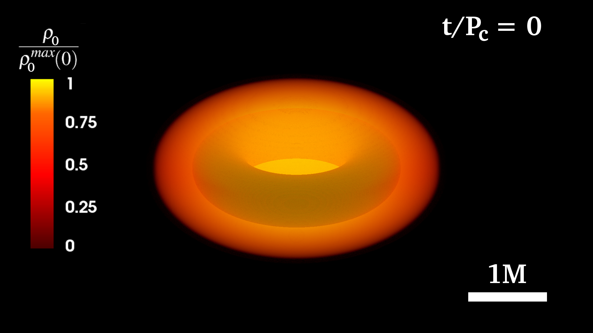
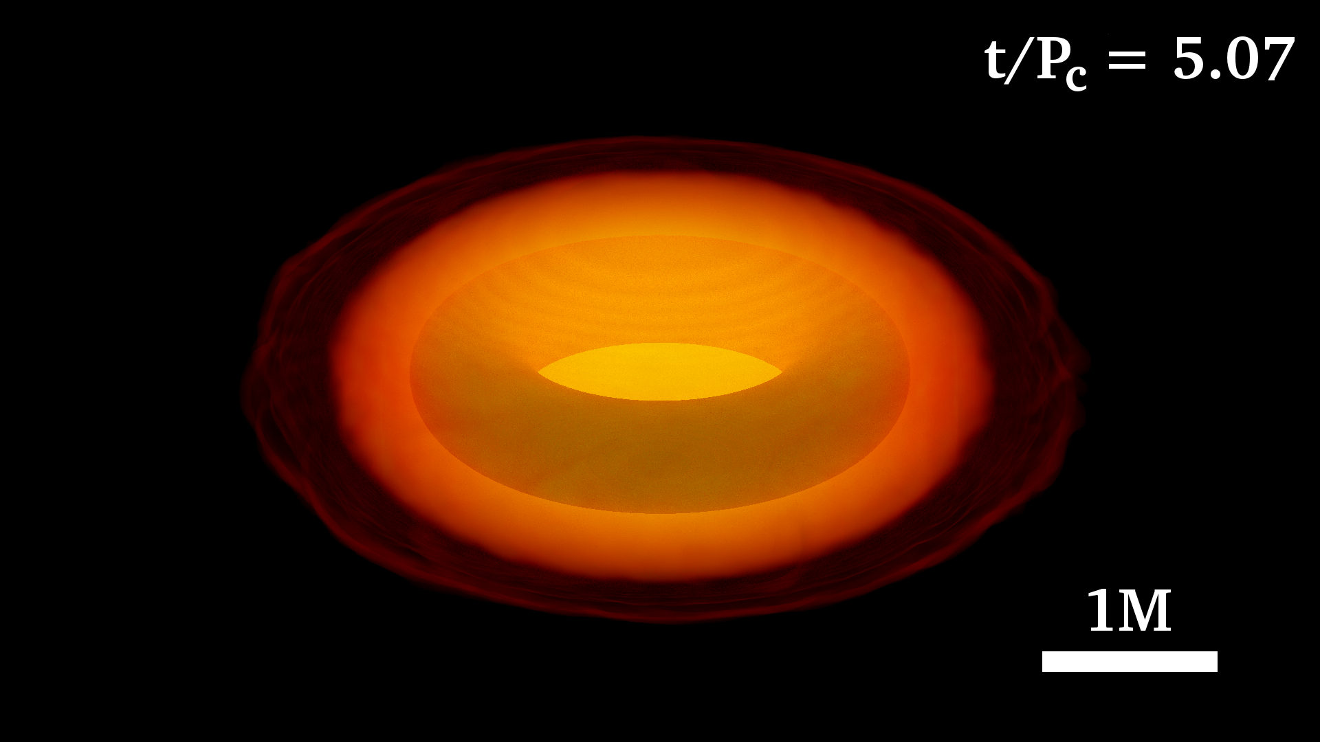
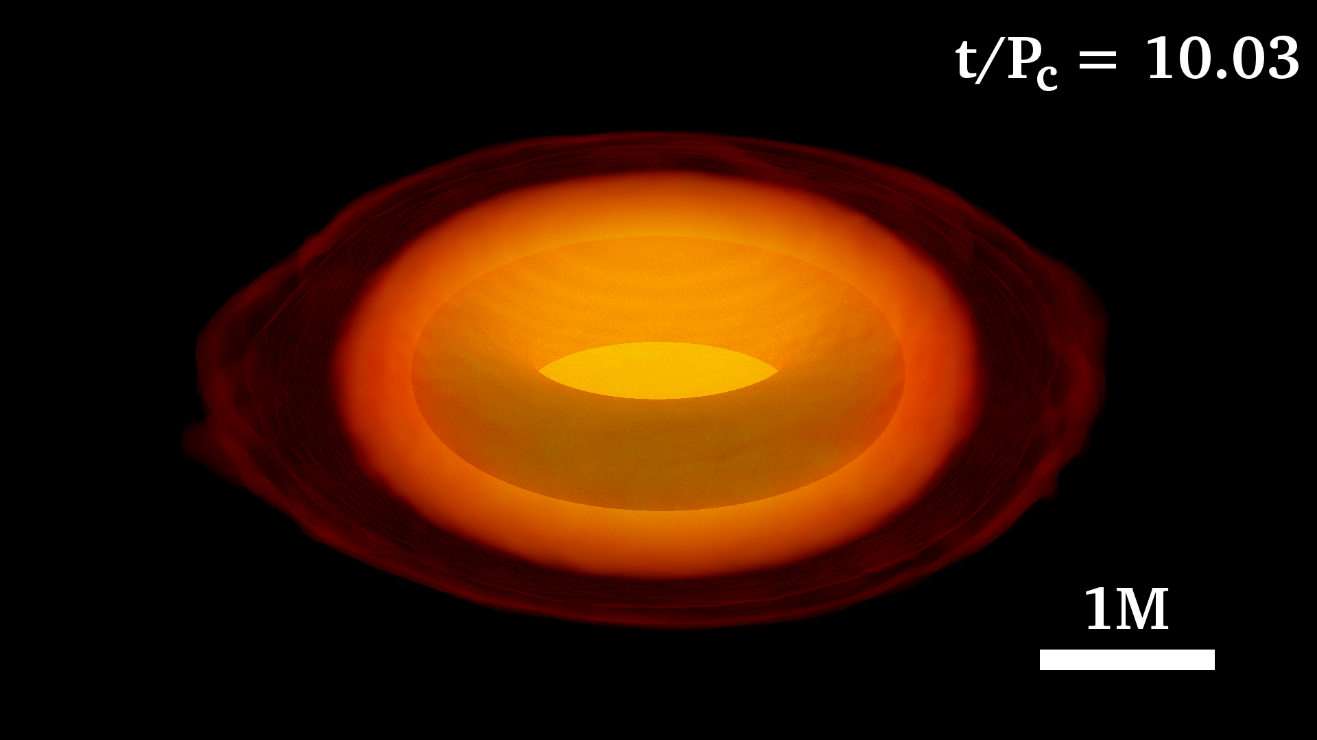
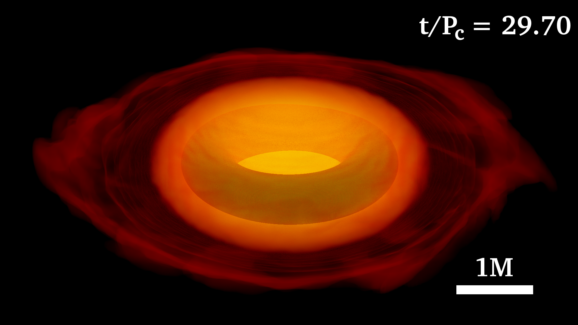
Figure 1: Rest-mass density and the ergosurface for the ALF2cc EoS, model iA0.2-rp0.45, at 4 different instances of time. The green donut indicates the ergoregion. Stability is maintained for this equilibrium ergostar.

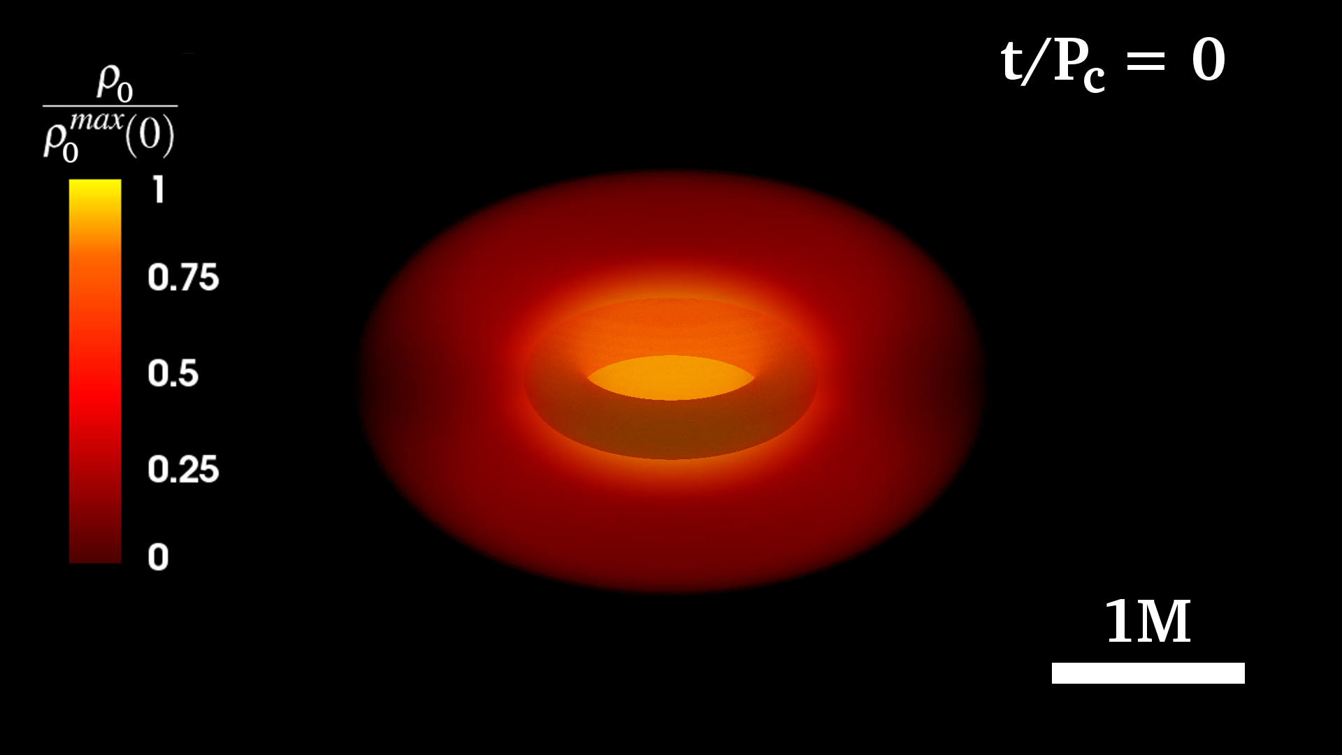
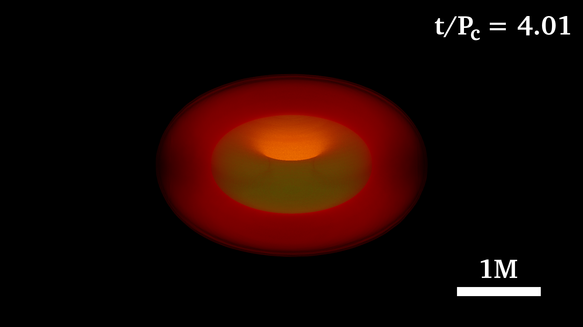
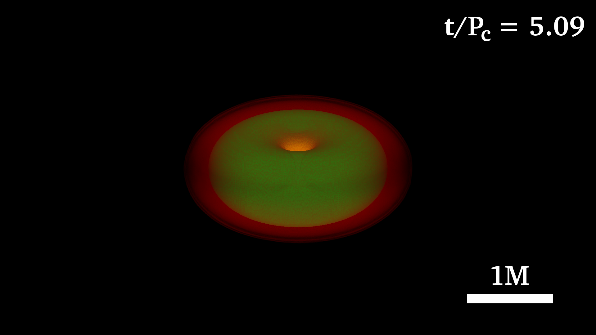
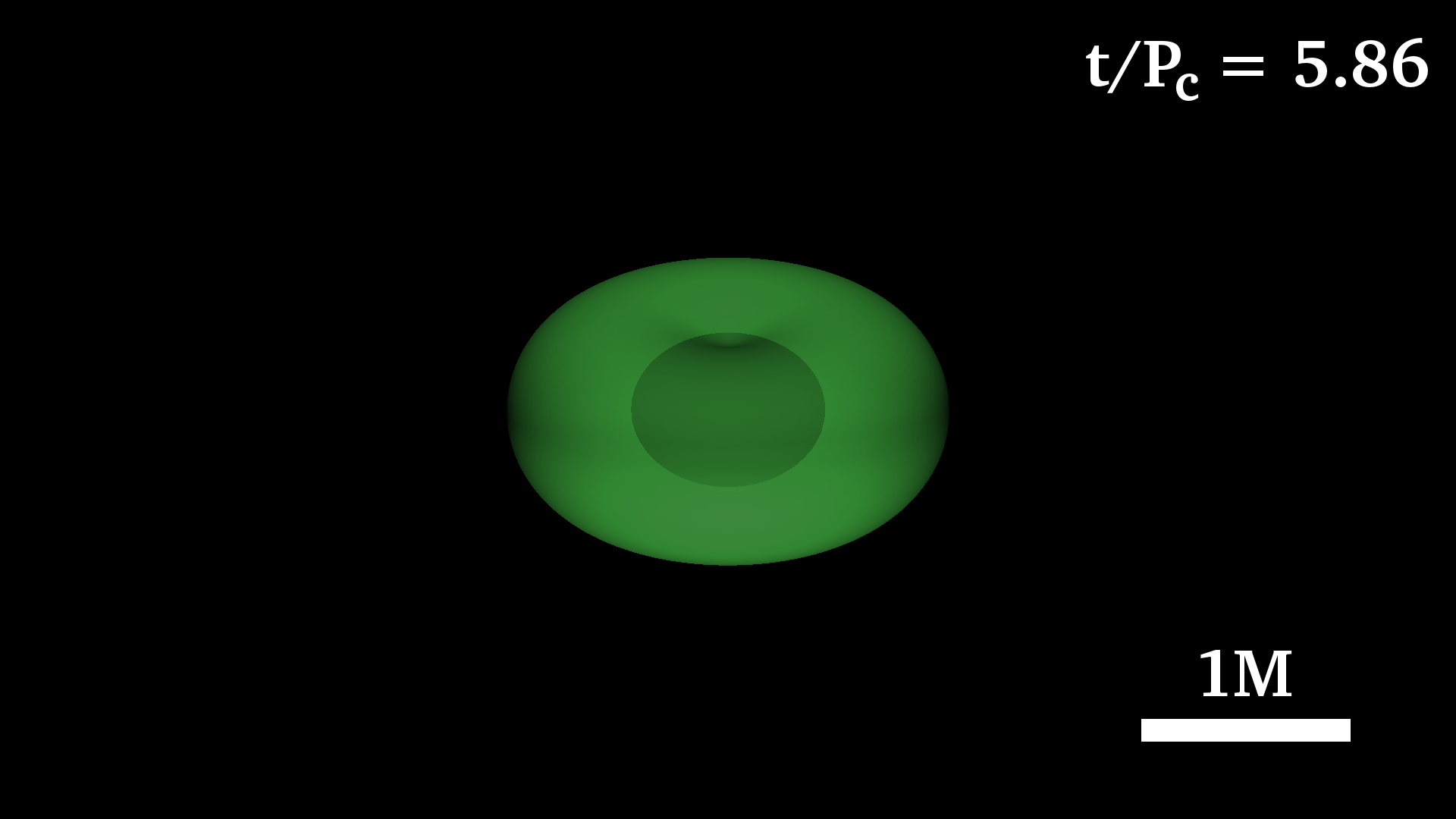
Figure 2: Similar to Fig. 1 but for the $\Gamma=3$ EoS model g3-iA0.4-rp0.42. This equilibrium ergostar undergoes dynamical collapse to a BH. The black inner spheroid in the last frame shows the apparent horizon.

Evolutions.—We use the Illinois GRMHD adaptive-mesh-refinement code (see e.g. Etienne et al. (2010)), which employs the Baumgarte–Shapiro–Shibata–Nakamura (BSSN) formulation of the Einstein’s equations Shibata and Nakamura (1995); Baumgarte and Shapiro (1998) to evolve the spacetime with the standard puncture gauge conditions. The equations of hydrodynamics are solved in conservation-law form adopting high-resolution shock-capturing methods. The pressure is decomposed as a sum of a cold and a thermal part, $P=P_{\rm cold}+(\Gamma_{\rm th}-1)\rho_{0}(\epsilon-\epsilon_{\rm cold})$ where $P_{\rm cold},\epsilon_{\rm cold}$ are the pressure and specific internal energy as computed from the initial data EoS. They are calculated using either a polytropic pressure-density relation or Eq. (1). For the thermal part we take $\Gamma_{\rm th}=5/3$. The growth of nonaxisymmetric modes is monitored by computing $C_{m}=\int\rho_{0}u^{t}\sqrt{-g}e^{im\phi}d^{3}x$ Paschalidis et al. (2015). In our simulations we used two resolutions, for the ALF2cc models with $\Delta x_{\rm min}=153,\ 92$ m. For the $\Gamma=3$ models we used three resolutions with $\Delta x_{\rm min}=200,\ 140,\ 92$ m. Here $\Delta x_{\rm min}$ is the step interval at the finest refinement level. Note that for the same $\Delta x_{\rm min}$ there is more grid coverage across the star for the $\Gamma=3$ models because $R_{e}$ is greater.

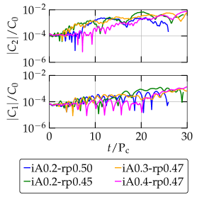
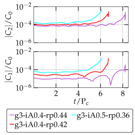
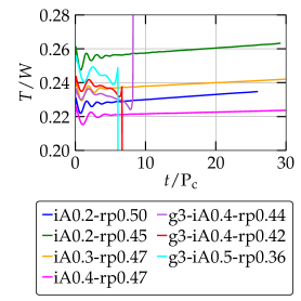
Figure 3: Time evolution of the $m=1,2$ modes for the ALF2cc EoS models (left panel), the $\Gamma=3$ EoS models (middle panel), and $T/W$ (right panel). The corresponding dynamical timescales are listed in Table 1.

Snapshots during the evolution of the ergostars with the ALF2cc and the $\Gamma=3$ EoSs are depicted in Figs. 1 and Fig. 2 where two prime examples of each category are plotted. Fig. 1 shows the normalized rest-mass density as well as the ergosurface ($g_{tt}=0$, inner green donut) of the model iA0.2-rp0.45 at 4 instances $t/{\rm P_{c}}\approx 0,\ 5,\ 10,\ 30$ and constitutes our prime, dynamically stable ergostar using the ALF2cc EoS that exhibits a causal core, Eq. (1). As it is clear from that figure the star retains both its axisymmetric structure as well as the geometry of the ergoregion for the whole period of our evolution that reaches approximately 30 rotation periods or 100 dynamical timescales. This ergostar is the first member that exhibits an ergoregion along a constant rest-mass (central) density $\rho_{0}=4.52\times 10^{14}\ {\rm gr/cm^{3}}$ sequence with a decreasing $R_{p}/R_{e}$ ratio and the j-const law with $\hat{A}=5$. All equilibrium models before that (i.e. for larger ratios of $R_{p}/R_{e}$) do not contain any ergoregions, while all models after that, i.e. for greater deformations (smaller ratios of $R_{p}/R_{e}$), contain ergoregions whose size increases with increasing deformation. In other words, for the particular sequence of rest-mass density and differential rotation law, ergostar iA0.2-rp0.45 is (a) the most spheroidal, (b) has the lowest $T/W$, and (c) has the smallest ergoregion. Note that $T/W=0.25$, which is certainly at the boundary of dynamical stability Baumgarte et al. (2000); Shibata et al. (2000). Less deformed models iA0.2-rp0.50 and iA0.2-rp0.47 belong to the same sequence as the ergostar iA0.2-rp0.45 and have the same differential rotation law but contain no ergoregions. These normal star equilibria have also a smaller value of $T/W$, and our simulations confirm that they are dynamically stable similarly.

Fig. 3 left panel, shows the growth of nonaxisymmetric modes for normal star iA0.2-rp0.50 as well as ergostars iA0.2-rp0.45, iA0.3-rp0.47, iA0.4-rp0.47 using $\Delta x_{\rm min}=153$ m. The same behavior is observed at higher resolution with $\Delta x_{\rm min}=92$ m. Evidently the evolution of all stars maintains axisymmetry on dynamical timescales. Particularly during the last 10 rotation periods both the normal star iA0.2-rp0.50 and the ergostar iA0.2-rp0.45 (which is shown also in Fig. 1) show a saturation of the $m=1,2$ growth amplitude. Ergostars iA0.3-rp0.47 and iA0.4-rp0.47 have the same central density as iA0.2-rp0.45 but larger differential rotation: $\hat{A}=3.33$ and $2.5$ respectively. In the Supplement we present additional evidence for the dynamical stability of these models by seeding them with an $m=1$ or $m=2$ density perturbation and inspecting their non-growth in the timescale of our simulations. In addition we show that these stars are stable to quasiradial density perturbations.

Fig. 2 shows the normalized rest-mass density and ergosurface for the $\Gamma=3$ EoS ergostar g3-iA0.4-rp0.42 evolved using $\Delta x_{\rm min}=200$ m at 4 instances $t/{\rm P_{c}}\approx 0,\ 4,\ 5$, and at BH formation. Although the criterion $\mathbf{t}\cdot\mathbf{t}=g_{tt}=0$ (where $\mathbf{t}=\partial_{t}$ is the time coordinate basis vector) for ergoregion identification does not strictly hold in the nonstationary spacetime of the collapsing star, it is still a reasonable measure given the stationary initial and final gravitational equilibria. This model is the first member that exhibits an ergoregion along a constant rest-mass density $\rho_{0}=3.846\times 10^{14}\ {\rm gr/cm^{3}}$ sequence with $\hat{A}=2.5$. All equilibrium models with less deformation do not contain any ergoregions, while all models with larger deformations contain larger size ergoregions. Also ergostar g3-iA0.4-rp0.42 is less deformed and has smaller $T/W$ than any of the $\Gamma=3$ models of Ref. Komatsu et al. (1989), therefore is less prone to bar-mode instabilities. Other models in Ref. Komatsu et al. (1989) containing ergoregions have very small ratios of $R_{p}/R_{e}$ and much higher $T/W$, thus the possibility of being dynamically unstable as well is much higher. This was indeed proven recently in a select number of such extreme toroids in Espino et al. (2019). Fig. 3 middle panel shows the growth of nonaxisymmetric modes for the $\Gamma=3$ EoS models g3-iA0.4-rp0.44 (normal star), g3-iA0.4-rp0.42 (ergostar shown in Fig. 2) and g3-iA0.5-rp0.36 (also an ergostar) until just after BH formation. The small values of $C_{m}/C_{0}$ imply the free-fall collapse of those models is axisymmetric. The resolution used is $\Delta x_{\rm min}=140$ m. In the right panel of Fig. 3 we plot $T/W$ for all the models discussed above. As it is evident the $\Gamma=3$ models all collapse while $T/W$ slightly decreases from their initial values. Also ergostar iA0.2-rp0.45 has the largest $T/W$ in the ALF2cc EoS set of models while the ergostar with the highest degree of differential rotation, iA0.4-rp0.47, has the smallest. The radial instability of the $\Gamma=3$ EoS models of Table 1 is verified by using three different resolutions with the highest one having $\Delta x_{\rm min}=92$ m. The evolution of the shape of the ergosphere for the model g3-iA0.4-rp0.42 is presented in the Supplement.

Discussion.—In this Letter we presented dynamically stable equilibrium rotating NSs that contain ergoregions. The EoS that we employed is causal at the core and ALF2 at the outer layers of the star. We also proved that previously calculated polytropic ergostars are dynamically unstable. The secular evolution of our models will probably be determined by the Friedman instability Friedman (1978a) in the absence of other dissipative mechanisms. Despite that, and given the long timescales involved, the possibility of existence of such equilibria raises a number of questions, the most obvious of them being the fate of ergostars exhibiting internal dissipative mechanisms, such as viscosity or magnetic fields (which may serve as turbulent viscosity). Preliminary calculations of magnetic effects in fixed spacetimes Ruiz et al. (2012) have shown that such systems can launch jets similar to BHs surrounded by magnetized disks. If the merger of two NSs forms an ergostar remnant which can launch a jet, the timescale for jet formation will be earlier than the one for a normal hypermassive NS Ruiz et al. (2016, 2018). This feature may have consequences in the theoretical analysis of events like GW170817 and its short gamma-ray burst counterpart GRB 170817A. Such open problems, as well as questions related to the range of EoSs and differential rotating laws that can lead to ergostars, or the possibility of binary ergostar remnants, are under investigation.

Movies highlighting results of our simulations can be found at http://research.physics.illinois.edu/ cta/movies/Ergostar/.

Acknowledgments.—It is a pleasure to thank R. Haas and V. Paschalidis for useful discussions. We also thank the Illinois Relativity group REU team, G. Liu, K. Nelli, and M. N.T Nguyen for assistance in creating Figs. 1 and 2. This work was supported by NSF grant PHY-1662211 and NASA grant 80NSSC17K0070 to the University of Illinois at Urbana-Champaign, as well as by JSPS Grant-in-Aid for Scientific Research (C) 15K05085 and 18K03624 to the University of Ryukyus. This work made use of the Extreme Science and Engineering Discovery Environment (XSEDE), which is supported by National Science Foundation grant number TG-MCA99S008. This research is part of the Blue Waters sustained-petascale computing project, which is supported by the National Science Foundation (awards OCI-0725070 and ACI-1238993) and the State of Illinois. Blue Waters is a joint effort of the University of Illinois at Urbana-Champaign and its National Center for Supercomputing Applications. Re-sources supporting this work were also provided by the NASA High-End Computing (HEC) Program through the NASA Advanced Supercomputing (NAS) Division at Ames Research Center.

I Supplemental Material

II Numerical stability analysis

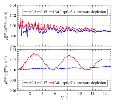
Figure 4: Top panel: model iA0.2-rp0.45. Maximum density evolution for the equilibrium configuration as well as the one with pressure depletion. Bottom panel: similarly for model iA0.4-rp0.47.

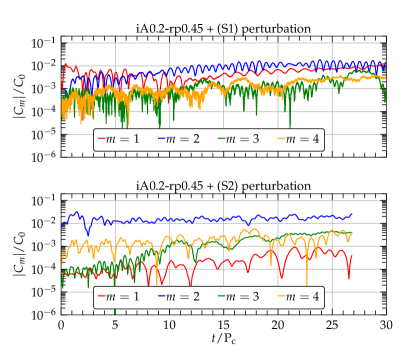
Figure 5: Top panel: mode growth for the model iA0.2-rp0.45 seeded with an $m=1$ perturbation. Bottom panel: similarly for an $m=2$ perturbation.

In this section we further probe the dynamical stability of our ergostar models iA0.2-rp0.45, iA0.3-rp0.47, iA0.4-rp0.47 by exciting a number of density perturbations in them. By applying an $m=0$ perturbation we investigate the stability against quasiradial oscillations, while an $m=1$ or $m=2$ perturbation tests the stability against nonaxisymmetric modes. The $m=0$ case is implemented by depleting the pressure in the stars by a certain amount which we chose to be $1\%$. The $m=1$ perturbation is implemented by modifying the density profile according to

$$\rho_{0}\rightarrow\rho_{0}\left(1+B\frac{x+y}{R_{\rm eq}}\right)\ ,$$ (S1)

where $R_{e}$ is the equatorial radius of the star, and $B$ a constant that we take to be $5\%$. Finally, the $m=2$ perturbation is applied by the use of the transformation

$$\rho_{0}\rightarrow\rho_{0}\left(1+B\frac{x^{2}-y^{2}}{R_{\rm eq}^{2}}\right)\ ,$$ (S2)

for the same choice of $B$. In order to isolate the effects that are coming from the ergoregion we apply the same perturbations to the regular stars iA0.2-rp0.50, iA0.2-rp0.47 that do not contain an ergoregion. Overall all our models behave in the same stable way and we could not identify any peculiar behavior that could in principle be attributed to the existence of the ergoregion.

In Fig. 4 we show the maximum density evolution for the equilibrium as well as the pressure-depletted stars iA0.2-rp0.45 (top panel) and iA0.4-rp0.47 (bottom panel). The equilibrium models do not exhibit any significant oscillations, therefore the pressure-depleted ones are stable as well. The featured ergostar, Fig. 1, whose maximum density coincides with its geometric center, exhibits very small oscillations when pressure depleted. On the other hand star iA0.4-rp0.47 whose maximum density is off-center oscillates more. Also, the slight increase in the density for the equilibrium model is due to numerical viscosity, as proved by evolving with different resolutions. Overall, all models in Table I present the same behavior when we pressure-deplete them, therefore they are all stable against quasiradial perturbations on dynamical timescales.

In Fig. 5 we present the effects of the $m=1$ one-arm perturbation Eq. (S1) in the top panel, and the effects of the $m=2$ bar-mode perturbation Eq. (S2) in the bottom panel, for the featured ergostar iA0.2-rp0.45. Plotted is the evolution of the first four modes. Model iA0.2-rp0.45 has the largest $T/W$ and therefore is more prone to the bar-mode instability. In addition as we can see from Fig. 3, right panel, this ergostar has $T/W(t>20{\rm P_{c}})>0.26$ which in turn suggests that when a bar mode is excited the possibility of exponential growth on a dynamical timescale is significant. The bottom panel of Fig. 5 shows that this intuition is mistaken. The $m=2$ perturbation shows no sign of growth whatsoever for the time of our integrations. The mode that mostly grows is the $m=3$ but still it has a small amplitude. The excitation of an $m=1$ mode on the other hand instigates the development of an $m=2$ mode as well. Both modes grow at the level of $1\%$ by the end of our simulations and, as seen in Fig. 5, they also show no sign of exponential growth. Almost identical behavior is observed in all models of Table I with the ALF2cc EoS. The facts that we do not observe any essential growth of any modes, as well as there is no geometrical or topological change of the equilibrium models for many dynamical times leads us to conclude that all of our ALF2cc stars are dynamically stable.

III Ergosphere evolution

Fig. 6 shows the ergosurface at 6 different instances of time for the collapsing ergostar g3-iA0.4-rp0.42 shown in Fig. 2. The ergoregion smoothly transitions from a toroidal to a spheroidal topology around $t\approx 5.6\ {\rm P_{c}}$, while the apparent horizon appears at $t=5.83\ {\rm P_{c}}$. The final BH has $a:=J/M^{2}=0.87$ which coincides with the corresponding value of the ergostar in Table I.

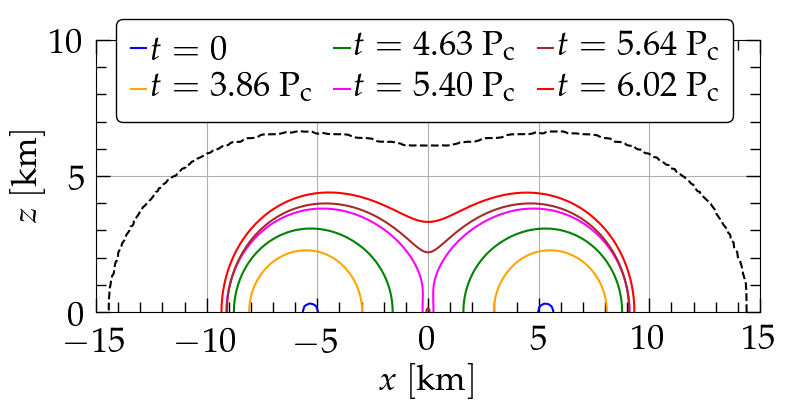
Figure 6: Ergoregion contours at different times for collapsing ergostar g3-iA0.4-rp0.42. The blue contour ($t=0$) shows the ergoregion for the initial data while the red contour ($t=6.02\ {\rm P_{c}}$) corresponds to the ergoregion of the final stationary BH. Black dashed line depicts initial star surface.

References

- Penrose (1969) R. Penrose, Riv. Nuovo Cim. 1, 252 (1969), [Gen. Rel. Grav.34,1141(2002)].
- Blandford and Znajek (1977) R. D. Blandford and R. L. Znajek, Monthly Notices of the Royal Astronomical Society 179, 433 (1977).
- Thorne et al. (1986) K. S. Thorne, R. H. Price, and D. A. Macdonald, The Membrane Paradigm (Yale University Press, New Haven, 1986).
- Komissarov (2004) S. S. Komissarov, Mon. Not. Roy. Astron. Soc. 350, 407 (2004), arXiv:astro-ph/0402403 .
- Komissarov (2005) S. S. Komissarov, mnras 359, 801 (2005), arXiv:astro-ph/0501599 .
- Ruiz et al. (2012) M. Ruiz, C. Palenzuela, F. Galeazzi, and C. Bona, Mon.Not.Roy.Astron.Soc. 423, 1300 (2012).
- Friedman (1978a) J. L. Friedman, Communications in Mathematical Physics 63, 243 (1978a).
- Moschidis (2018) G. Moschidis, Communications in Mathematical Physics 358, 437 (2018), arXiv:1608.02035 [math.AP] .
- Chandrasekhar (1970) S. Chandrasekhar, Astrophys. J. 161, 561 (1970).
- Friedman and Schutz (1978) J. L. Friedman and B. F. Schutz, Astrophys. J. 221, 937 (1978).
- Friedman (1978b) J. L. Friedman, Communications in Mathematical Physics 62, 247 (1978b).
- Comins and Schutz (1978) N. Comins and B. F. Schutz, Proceedings of the Royal Society of London Series A 364, 211 (1978).
- Yoshida and Eriguchi (1996) S. Yoshida and Y. Eriguchi, Monthly Notices of the Royal Astronomical Society 282, 580 (1996).
- Brito et al. (2015) R. Brito, V. Cardoso, and P. Pani, Lect. Notes Phys. 906, pp.1 (2015), arXiv:1501.06570 [gr-qc] .
- Kokkotas et al. (2004) K. D. Kokkotas, J. Ruoff, and N. Andersson, Phys. Rev. D70, 043003 (2004), arXiv:astro-ph/0212429 [astro-ph] .
- Schutz and Comins (1978) B. F. Schutz and N. Comins, Monthly Notices of the Royal Astronomical Society 182, 69 (1978).
- Wilson (1972) J. R. Wilson, Astrophys. J. 176, 195 (1972).
- Butterworth and Ipser (1975) E. M. Butterworth and J. R. Ipser, Astrophys. J. 200, L103 (1975).
- Ansorg et al. (2002) M. Ansorg, A. Kleinwachter, and R. Meinel, Astron. Astrophys. 381, L49 (2002), arXiv:astro-ph/0111080 [astro-ph] .
- Ames et al. (2019) E. Ames, H. Andréasson, and A. Logg, Phys. Rev. D99, 024012 (2019), arXiv:1803.11224 [gr-qc] .
- Ames et al. (2016) E. Ames, H. Andréasson, and A. Logg, Class. Quant. Grav. 33, 155008 (2016), arXiv:1603.05404 [gr-qc] .
- Komatsu et al. (1989) H. Komatsu, Y. Eriguchi, and I. Hachisu, Monthly Notices of the Royal Astronomical Society 239, 153 (1989).
- Cook et al. (1992) G. B. Cook, S. L. Shapiro, and S. A. Teukolsky, Astrophys. J. 398, 203 (1992).
- Alford et al. (2005) M. Alford, M. Braby, M. Paris, and S. Reddy, Astrophys. J. 629, 969 (2005), nucl-th/0411016 .
- Lattimer and Prakash (2016) J. M. Lattimer and M. Prakash, Phys. Rept. 621, 127 (2016).
- Tsokaros et al. (2019) A. Tsokaros, M. Ruiz, S. Lunan, L. S. Shapiro, and K. Uryū, In preparation (2019).
- Eriguchi and Mueller (1985) Y. Eriguchi and E. Mueller, aap 146, 260 (1985).
- Uryū et al. (2016) K. Uryū, A. Tsokaros, F. Galeazzi, H. Hotta, M. Sugimura, K. Taniguchi, and S. Yoshida, Phys. Rev. D93, 044056 (2016).
- Uryu et al. (2017) K. Uryu, A. Tsokaros, L. Baiotti, F. Galeazzi, K. Taniguchi, and S. Yoshida, Phys. Rev. D96, 103011 (2017), arXiv:1709.02643 [astro-ph.HE] .
- Etienne et al. (2010) Z. B. Etienne, Y. T. Liu, and S. L. Shapiro, Phys.Rev. D82, 084031 (2010).
- Shibata and Nakamura (1995) M. Shibata and T. Nakamura, Phys. Rev. D 52, 5428 (1995).
- Baumgarte and Shapiro (1998) T. W. Baumgarte and S. L. Shapiro, prd 59, 024007 (1998).
- Paschalidis et al. (2015) V. Paschalidis, W. E. East, F. Pretorius, and S. L. Shapiro, Phys. Rev. D92, 121502 (2015), arXiv:1510.03432 [astro-ph.HE] .
- Baumgarte et al. (2000) T. W. Baumgarte, S. L. Shapiro, and M. Shibata, Astrophys. J. 528, L29 (2000), arXiv:astro-ph/9910565 [astro-ph] .
- Shibata et al. (2000) M. Shibata, T. W. Baumgarte, and S. L. Shapiro, The Astrophysical Journal 542, 453 (2000).
- Espino et al. (2019) P. L. Espino, V. Paschalidis, T. W. Baumgarte, and S. L. Shapiro, Phys. Rev. D100, 043014 (2019), arXiv:1906.08786 [astro-ph.HE] .
- Ruiz et al. (2016) M. Ruiz, R. N. Lang, V. Paschalidis, and S. L. Shapiro, Astrophys. J. 824, L6 (2016).
- Ruiz et al. (2018) M. Ruiz, S. L. Shapiro, and A. Tsokaros, Phys. Rev. D98, 123017 (2018), arXiv:1810.08618 [astro-ph.HE] .