LocationSpark: In-memory Distributed Spatial Query Processing and Optimization
Abstract
Due to the ubiquity of spatial data applications and the large amounts of spatial data that these applications generate and process, there is a pressing need for scalable spatial query processing. In this paper, we present new techniques for spatial query processing and optimization in an in-memory and distributed setup to address scalability. More specifically, we introduce new techniques for handling query skew, which is common in practice, and optimize communication costs accordingly. We propose a distributed query scheduler that use a new cost model to optimize the cost of spatial query processing. The scheduler generates query execution plans that minimize the effect of query skew. The query scheduler employs new spatial indexing techniques based on bitmap filters to forward queries to the appropriate local nodes. Each local computation node is responsible for optimizing and selecting its best local query execution plan based on the indexes and the nature of the spatial queries in that node. All the proposed spatial query processing and optimization techniques are prototyped inside Spark, a distributed memory-based computation system. The experimental study is based on real datasets and demonstrates that distributed spatial query processing can be enhanced by up to an order of magnitude over existing in-memory and distributed spatial systems.
Index Terms:
spatial data, query processing, in-memory computation, parallel computing1 Introduction
Spatial computing is becoming increasingly important with the proliferation of mobile devices. In addition, the growing scale and importance of location data have driven the development of numerous specialized spatial data processing systems, e.g., SpatialHadoop [9], Hadoop-GIS [3] and MD-Hbase [17]. By taking advantage of the power and cost-effectiveness of MapReduce, these systems typically outperform spatial extensions on top of relational database systems by orders of magnitude [3]. MapReduce-based systems allow users to run spatial queries using predefined high-level spatial operators without worrying about fault tolerance or computation distribution. However, these systems have the following two main limitations: (1) they do not leverage the power of distributed memory, and (2) they are unable to reuse intermediate data [26]. Nonetheless, data reuse is very common in spatial data processing. For example, spatial datasets, e.g., Open Street Map (OSM, for short, 60G) and Point of Interest (POI, for short, 20G) [9], are usually large. It is unnecessary to read these datasets continuously from disk (e.g., using HDFS [19]) to respond to user queries. Moreover, intermediate query results have to be written back to HDFS, thus directly impeding the performance of further data analysis steps.
One way to address the above challenges is to develop an efficient execution engine for large-scale spatial data computation based on a memory-based computation framework (in this case, Spark [26]). Spark is a computation framework that allows users to work on distributed in-memory data without worrying about data distribution or fault-tolerance. Recently, various Spark-based systems have been proposed for spatial data analysis, e.g., SpatialSpark [2], GeoSpark [25], Magellan [1], Simba [24] and LocationSpark [21].
Although addressing several challenges in spatial query processing, none of the existing systems is able to overcome the computation skew introduced by spatial queries. “Spatial query skew” is observed in distributed environments during spatial query processing when certain data partitions are overloaded by spatial queries. Traditionally, distributed spatial computing systems (e.g., [9, 3, 2]) first learn the spatial data distribution by sampling the input data. Afterwards, spatial data is evenly partitioned into equal-size partitions. For example, in Figure 1, the data points with dark dots are evenly distributed into four partitions. Given the partitioned data, consider two spatial join operators, namely range and NN joins, to combine two datasets, say and , with respect to a spatial relationship. For each point , a spatial range join (Figure 1(a)) returns data points in that are inside the radius of the circle centered at . In contrast, a NN join (Figure 1(b)) returns the nearest-neighbors from the dataset for each query point . Both spatial operators are expensive and may incur computation skew in certain workers, thus greatly degrading the overall performance.
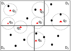
For illustration, consider a large spatial dataset, with millions of points of interests (POIs), that is partitioned into different computation nodes based on the spatial distribution of the data, e.g., one data partition represents data from San Francisco, CA, and another one for Chicago, IL. Assume that we have incoming queries from people looking for different POIs, e.g., restaurants, train or bus stations, and grocery stores, around their locations. These spatial range queries are consolidated into batches to be joined via an index on the POI data (e.g., using indexed nested-loops join). After partitioning the incoming spatial queries based on their locations, we observe the following issues: During rush hours in San Francisco from 4PM to 6PM (PST), San Francisco’s data partition may encounter more queries than the data partition in Chicago, since it is already the evening in Chicago. Without an appropriate optimization technique, the data partition for San Francisco will take much longer time to process its corresponding queries while the workers responsible for the other partitions are lightly loaded. As another example, in Figure 1, the data points (the dark dots) correspond to Uber car’s GPS records where multiple users (the triangles) are looking for the Uber carpool service around them. Partition , which corresponds to an airport, experiences more queries than other partitions because people may prefer using Uber at this location. Being aware of the spatial query skew provides a new opportunity to optimize queries in distributed spatial data environments. The skewed partitions have to be assigned more computation power to reduce the overall processing time.
Furthermore, communication cost, generally a key factor of the overall performance, may become a bottleneck. When a spatial query touches more than one data partition, it may be the case that some of these partitions do not contribute to the final query result. For example, in Figure 1(a), queries , , , and overlap more than one data partition (, , and ), but these partitions do not contain data points that satisfy the queries. Thus, scheduling queries (e.g., and ) to the overlapping data partition incurs unnecessary communication cost. More importantly, for the spatial range join or NN join operators over two large datasets, the cost of network communication may become prohibitive without proper optimization.
In this paper, we introduce LocationSpark, an efficient memory-based distributed spatial query processing system. In particular, it has a query scheduler to mitigate query skew. The query scheduler uses a cost model to analyze the skew for use by the spatial operators, and a plan generation algorithm to construct a load-balanced query execution plan. After plan generation, local computation nodes select the proper algorithms to improve their local performance based on the available spatial indexes and the registered queries on each node. Finally, to reduce the communication cost when dispatching queries to their overlapping data partitions, LocationSpark adopts a new spatial bitmap filter, termed sFilter, that can speed up query processing by avoiding needless communication with data partitions that do not contribute to the query answer. We implement LocationSpark as a library in Spark that provides an API for spatial query processing and optimization based on Spark’s standard dataflow operators.
The main contributions of this paper are as follows:
-
1.
We develop a new spatial computing system for efficient processing of spatial queries in a distributed in-memory environment.
-
2.
We address data and query skew issues to improve load balancing while executing spatial operators, e.g., spatial range joins and NN joins, by generating cost-optimized query execution plans over in-memory distributed spatial data.
-
3.
We introduce a new lightweight yet efficient spatial bitmap filter to reduce communication cost.
-
4.
We realize the introduced query processing and optimization techniques inside Spark. We use the developed prototype system, LocationSpark, to conduct a large-scale evaluation on real spatial data and common benchmark algorithms, and compare LocationSpark against state-of-the-art distributed spatial data processing systems. Experimental results illustrate an enhancement in performance by up to an order of magnitude over existing in-memory distributed spatial systems.
The rest of this paper proceeds as follows. Section 2 presents the problem definition and an overview of distributed spatial query processing. Section 3 introduces the cost model and the cost-based query plan scheduler and optimizer and their corresponding algorithms. Section 4 presents an empirical study for local execution plans in local computation nodes. Section 5 introduces the spatial bitmap filter, and explains how it can speedup spatial query processing in a distributed setup. The experimental results are presented in Section 6. Section 7 discusses the related work. Finally, Section 8 concludes the paper.
2 Preliminaries
2.1 Data Model and Spatial Operators
LocationSpark stores spatial data as key-value pairs. A tuple, say , contains a spatial geometric key and a related value . The spatial data type for key can be a two-dimensional point, e.g., latitude-longitude, a line-segment, a poly-line, a rectangle, or a polygon. The value type is specified by the user, e.g., a text data type if the data tuple is a tweet. In this paper, we assume that queries are issued continuously by users, and are processed by the system in batches (i.e., similar to the DStream model [26]).
LocationSpark supports various types of spatial query predicates including spatial range search, -NN search, spatial range join, and NN join. In this paper, we focus our discussions on the spatial range join and NN join operators on two dataset, say and , which form the outer and inner tables, respectively.
Definition 1
Spatial Range Search - : Given a spatial range area (e.g., circle or rectangle) and a dataset , finds all tuples from that overlap the spatial range defined by .
Definition 2
Spatial Range Join - : Given two dataset and , , combines each object with its range search results from , = .
Definition 3
NN Search - NN(q,D): Given a query tuple , a dataset , and an integer , NN(q,D), returns the output set and and , where the number of output objects from , = .
Definition 4
NN Join - : Given a parameter , NN join of and computes each object with its nearest neighbors from . = .
2.2 Overview of In-memory Distributed Spatial Query Processing
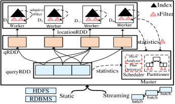
To facilitate spatial query processing, we build a distributed spatial index for in-memory spatial data. Given a spatial dataset , we obtain samples from and construct a spatial index (e.g., an R-tree) with leaves over the samples. We refer to this index on the sample data as the global spatial index. Next, each worker partitions the dataset into partitions according to the built global spatial index via data shuffling. The global spatial index guarantees that each data partition approximately has the same amount of data. Then, each worker of the workers has a local data partition that is roughly th of the data and builds a local spatial index. Finally, the indexed data (termed the LocationRDD) is cached into memory. Figure 2 gives the architecture of LocationSpark and the physical representation of the partitioned spatial data based on the procedure outlined above, where the master node stores the global spatial index that indexes the data partitions, while each worker has a local spatial index over the local spatial data within the partition. Notice that the global spatial index partitions the data into LocationRDDs as in Figure 2, and this index can be copied into various workers to help partition the data in parallel. The type of each local index, e.g., a Grid, an R-tree, or an IR-tree, for a data partition can be determined based on the specifics of the application scenarios. For example, a Grid can be used for moving objects indexing while an R-tree can be used for polygons objects.
For spatial range join, two strategies are possible; either replicate the outer table and send it to the node where the inner table is or replicate the inner table data and send it to the different processing nodes where the outer table tuples are. In a shared execution, the outer table is typically a collection of range query tuples and the inner table is the queried dataset. If this is the case, it would make more sense to send the outer table of queries to the inner data tables as the outer table is usually much smaller compared to the inner data tables. In this paper, we adopt the first approach because it would be impracticable to replicate and forward copies of the large inner data table.
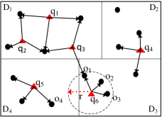
Thus, each tuple is replicated and forwarded to the partitions that spatially overlap with it. These overlapping partitions are identified using the global index. Then, a post-processing step merges the local results to produce the final output. For example, we replicate the outer table in Figure 1(a) and forwarded it to data partitions , , and . Then, we execute a spatial range search on each data partition locally. Next, we merge the local results to form the overall output of tuple . As illustrated in Figure 2, the outer table that corresponds to a shared execution plan’s collection of queries (termed queryRDD) are first partitioned into qRDD based on the overlap between the queries in qRDD and the corresponding data partitions. Then, local search takes place over the local data partitions of LocationRDD.
The NN join operator is implemented similarly in a simple two-round process. First, each outer focal points is transferred to the worker that holds the data partition that spatially belongs to. Then, the NN join is executed locally in each data partition, producing the NN candidates for each focal point . Afterwards, the maximum distance from to its NN candidates, say radius , is computed. If the radius overlaps multiple data partitions, point is replicated into these overlapping partitions, and another set of NN candidates is computed in each of these partitions. Finally, we merge the NN candidates from the various partitions to get the exact result. For example, in Figure 1(b), assume that we want to evaluate a NN query for Point . The first step is to find the NN candidates for in data Partition . Next, we find that the radius for the NN candidates from Partition overlaps Partition . Thus, we need to compute the NN of in Partition as well. Notice that the radius can enhance the NN search in Partition because only the data points within Radius are among the NN of . Finally, the NN of are , and .
2.3 Challenges
The outer and inner tables (or, in shared execution terminology, the queries and the data) are spatially collocated in distributed spatial computing. In the following discussion, we refer to the outer table as being the queries table, e.g., containing the ranges of range operations, or the focal points of NN operations. We further assume that the outer (or queries) table is the smaller of the two. We refer to the inner table by the data table (in the case of shared execution of multiple queries together). The distribution of the incoming spatial queries (in the outer tables) changes dynamically over time, with bursts in certain spatial regions. Thus, evenly distributing the input data to the various workers may result in load imbalance at times. LocationSpark’s scheduler identifies the skewed data partitions based on a cost model and then repartitions and redistributes the data accordingly, and selects the optimal repartitioning strategies for both the outer and inner tables, and consequently generates an overall optimized execution plan.
Communication cost is a major factor that affects system performance. LocationSpark adopts a spatial bitmap filter to reduce network communication cost. The spatial bitmap filter’s role is to prune the data partitions that overlap the spatial ranges from the outer tables but do not contribute to the final operation’s results. This spatial bitmap filter is memory-based and is space- and time-efficient. The spatial bitmap filter adapts its structure as the data and query distributions change.
3 Query Plan Scheduler
This section addresses how to dynamically handle query (outer table) skew. First, we present the cost functions for query processing and analyze the bottlenecks. Then, we show how to repartition the skewed data partitions to speedup processing. This is formulated as an optimization problem that we show is NP-complete. Consequently, we introduce an approximation algorithm to solve the skew data repartitioning problem. Although presented for spatial range joins, the proposed technique applies to NN join as well.
3.1 Cost Model
The input table (i.e., inner table of spatial range join) is distributed into data partitions, and each data partition is indexed and cached in memory. For the query table (i.e., outer table of spatial range join), each query is shuffled to the data partitions that spatially overlap with it. The shuffling cost is denoted by . The execution time of local queries at Partition is . The execution times of local queries depend on the queries and built indexes, and the estimation of is presented later. After the local results are computed, the post-processing step merges these local results to produce the final output. The corresponding cost is denoted by .
Overall, the runtime cost for the spatial range join operation is:
| (1) |
where is the number of data partitions. In reality, the cost of query shuffling is far less than the other costs as the number of queries is much smaller than the number of data items. Thus, the runtime cost can be estimated as follows:
| (2) |
We categorize the data partitions into two types: skewed () and non-skewed (). The execution time of the local queries in the skewed partitions is the bottleneck. The runtime costs for skewed and non-skewed data partitions are and , respectively, where (and ) is the number of skewed (and non-skewed) data partitions, and . Thus, Equation 2 can be rewritten as follows:
| (3) |
3.2 Execution Plan Generation
The goal of the query scheduler is to minimize the query processing time subject to the following constraints: (1) the limited number of available resources (i.e., the number of partitions) in a cluster, and (2) the overhead of network bandwidth and disk I/O. Given the partitioned and indexed spatial data, the cost estimator for query processing based on sampling that we introduce below, and the available number of data partitions, the optimizer returns an execution plan that minimizes query processing time. First, the optimizer determines if any partitions are skewed. Then, it repartitions them subject to the introduced cluster and networking constraints. Finally, the optimizer evaluates the plan on the newly repartitioned data to determine whether it minimizes query execution time or not (Refer to Figure 3).
Estimating the runtime cost of executing the local queries and the cost of merging the final results is not straightforward. The local query processing time is influenced by various factors including the types of spatial indexes used, the number of data points in , the number of queries directed to , related spatial regions, and the available memory. Similar to [13], we assume that the related cost functions are monotonic, and can be approximated using samples from the outer and inner tables (the queries and the datasets tables). Thus, the local query execution time is formulated as follows: , where is a sample of the original inner table dataset, is the sample of the outer table queries, is the area of the underlying spatial region, and is the sample ratio to scale up the estimate to the entire dataset. After computing a representative sample of the data points and queries, e.g., using reservoir sampling [22], the cost function estimates the query processing runtime in data partition . More details on computing , , and the sample size can be learned from previous work [13].
Given the estimated runtime cost over skewed and non-skewed partitions, the optimizer splits one skewed data Partition into data sub-partitions. Assume that is the set of queries originally assigned to Partition . Let the overheads due to data shuffling, re-indexing, and merging be , and , respectively. Thus, after splitting a skewed Partition , the new runtime is:
| (4) |
Hence, we can split one skewed Partition into multiple partitions only if . As a result, the new query execution time, say , is:
| (5) |
Thus, we can formulate the query plan generation based on the data repartitioning problem as follows:
Definition 5
Let be the set of spatially indexed data partitions, be the set of spatial queries, be the total number of data partitions, and their corresponding cost estimation functions, i.e., local query execution , data repartitioning , and data indexing cost estimates . The query optimization problem is to choose a skewed Partition from , repartition each into multiple partitions, and assign spatial queries to the new data partitions. The new data partition set, say , contains partitions . s.t. (1) and (2) .
Unfortunately, this problem is NP-complete. In the next section, we present a greedy algorithm for this problem.
Theorem 1
Optimized query plan generation with data repartitioning for distributed indexed spatial data is NP-complete.
The proof is given in [16].
3.3 A Greedy Algorithm
The general idea is to search for skewed partitions based on their local query execution time. Then, we split the selected data partitions only if the runtime can be improved. If the runtime cannot be improved, or if all the available data partitions are consumed, the algorithm terminates. While this greedy algorithm cannot guarantee optimal query performance, our experiments show significant improvement (by one order of magnitude) over the plan executing on the original partitions. Algorithm 1 gives the pseudocode for the greedy partitioning procedure.
Algorithm 1 includes two functions, namely numberOfPartitions and repartition. Function numberOfPartitions computes the number of partitions for splitting one skewed partition. Naively, we could split a skewed partition into two partitions each time. But this is not necessarily efficient. Given data partitions , let Partition be the one with the largest local query execution time . From Equation 2, the execution time is approximated by . To improve this execution time, Partition is split into partitions, and the query execution time for Partition is updated to . For all other partitions (), the runtime is the , where and are the queries related to all data partitions except . Thus, the runtime is , and is improved if
| (6) |
As a result, we need to compute the minimum value of to satisfy Equation 6, since , , and are known.
Function repartition splits the skewed data partitions and reassigns the spatial queries to the new data partitions using two strategies. The first strategy repartitions based on the data distribution. Because each data partition is already indexed by a spatial index, the data distribution can be learned directly by recording the number of data points in each branch of the index. Then, we repartition data points in into multiple parts based on the recorded numbers while guaranteeing that each newly generated sub-partition contains an equal amount of data. In the second strategy, we repartition a skewed Partition based on the distribution of the spatial queries. First, we collect a sample from the queries that are originally assigned to partition . Then, we compute how is distributed in Partition by recording the frequencies of the queries as they belong to branches of the index over the data. Thus, we can repartition the indexed data based on the query frequencies. Although the data sizes may not be equal, the execution workload will be balanced. In our experiments, we choose this second approach to overcome query skew. To illustrate how the proposed query-plan optimization algorithm works, consider the following example.
Running Example. Given data partitions , where the number of data points in each partition is 50, the number of queries in each partition , is 30, 20, 10, 10, and 10, respectively, and the available data partitions is 5. For simplicity, the local query processing cost is , where is a constant. The cost of merging the results is , where , and is the approximate number of retrieved data points per query. The cost of data shuffling and re-indexing after repartitioning is , and , respectively, where and . Without any optimization, from Equation 2, the estimated runtime cost for this input table is 340. LocationSpark optimizes the query as follows. At first, it chooses data Partition as the skewed partition to be repartitioned because has the highest local runtime (300), while the second largest cost is ’s (200). Using Equation 6, we split into two partitions, i.e., . Thus, Function repartition splits into the two partitions and based on the distribution of queries within . The number of data points in and is 22 and 28, respectively, and the number of queries are 12 and 18, respectively. Therefore, the new runtime is reduced to because ’s runtime is reduced to based on Equation 4. Therefore, the two new data partitions and are introduced in place of . Next, Partition is chosen to be split into two partitions, and the optimized runtime becomes . Finally, the procedure terminates as only one available partition is left.
4 Local Execution
Once the query plan is generated, each computation node chooses a specific local execution plan based on the queries assigned to it and the indexes it has. We implement various centralized algorithms for spatial range join and NN join operators within each worker and study their performance. The algorithms are implemented in Spark. We use the execution time as the performance measure.
4.1 Spatial Range Join
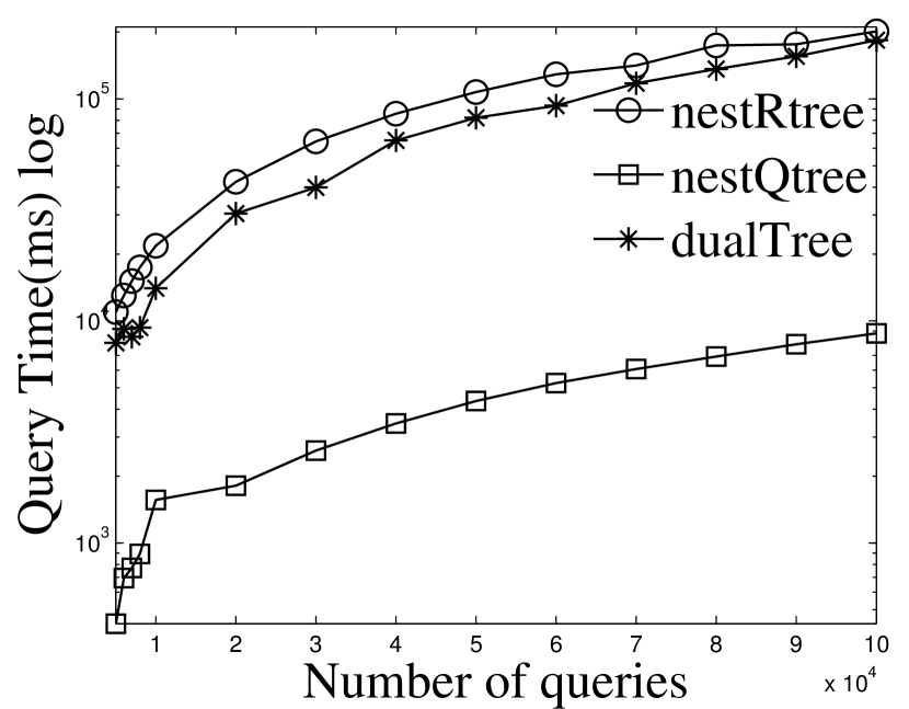
We implement two algorithms for spatial range join [20]. The first is indexed nested-loops join, where we probe the spatial index repeatedly for each outer tuple (or range query in the case of shared execution). The tested algorithms are nestRtree, nestGrid and nestQtree, where they use an R-tree, a Grid, and a Quadtree as index for the inner table, respectively. The second algorithm is based on the dual-tree traversal [6]. It builds two spatial indexes (e.g., an R-tree) over both the input queries and the data, and performs a depth-first search over the dual trees simultaneously.
Figure 4(a) gives the performance of nestRtree, nestQtree, and dual-tree, where the number of data points in each worker is 300K. The results for nestGrid are not given as it performs the worst. The dual-tree approach provides a 1.8x speedup over the nestRtree. This conforms with other published results [20]. nestQtree achieves an order of magnitude improvement over the dual-tree approach. The reason is that the minimum bounding rectangles (MBRs) of the spatial queries overlap with multiple MBRs in the data index, and this reduces the pruning power of the underlying R-tree. The same trend is observed in Figure 4(b) when increasing the number of indexed data points. The dual-tree approach outperforms nestRtree, when the number of data points is smaller than 120k. However, dual-tree slows down afterwards. In this experiment, we only show the results for indexing over two dimensional data points. However, Quadtree performs worst when the indexed data are polygons [18]. Overall, for multidimensional points, the local planner chooses nestQtree as the default approach. For complex geometric types, the local planner uses the dual-tree approach based on an R-tree implementation.
4.2 kNN Join
Similar to the spatial range join, indexed nested-loops can be applied to NN join, where it computes the set of NN objects for each query point in the outer table. An index is built on the inner table (the data table). The other kinds of NN join algorithms are block-based. They partition the queries (the outer table) and the data points (the inner table) into different blocks, and find the NN candidates for queries in the same block. Then, a post-processing refine step computes NN for each query point in the same block. Gorder [23] divides query and data points into different rectangles based on the G-order, and utilizes two distance bounds to reduce the processing of unnecessary blocks. For example, the min-distance bound is the minimum distance between the rectangles of the query points and the data points. The max-distance bound is the maximum distance from the queries to their NN sets. If the max-distance is smaller than the min-distance bound, the related data block is pruned. PGBJ [15] has a similar idea that extends to parallel NN join using MapReduce. Recently, Spitfire [8] is a parallel NN self-join algorithm for in-memory data. It replicates the possible NN candidates into its neighboring data blocks. Both PGBJ and Spitfire are designed for parallel NN join, but they are not directly applicable to indexed data. The reason is that PGBJ partitions queries and data points based on the selected pivots while Spitfire is specifically optimized for NN self-join.
LocationSpark enhances the performance of the local NN join procedure. For the Gorder [23], instead of using the expensive principal component analysis (PCA) in Gorder, we apply the Hilbert curve to partition the query points. We term the modified Gorder method sfcurve. We modify PGBJ as follows. First, we compute the pivots of the query points based on a clustering algorithm (e.g., k-means) over sample data, and then partition the query points into different blocks based on the computed pivots. Next, we compute the MBR of each block. Because the data points are already indexed (e.g., using an R-tree), the min-distance from the MBRs of the query points and the index data is computed, and the max-distance bound is calculated based on the NN results from the pivots. This approach is termed pgbjk. In terms of spitfire, we use a spatial index to speedup finding the NN candidates.
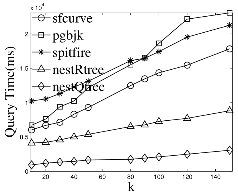
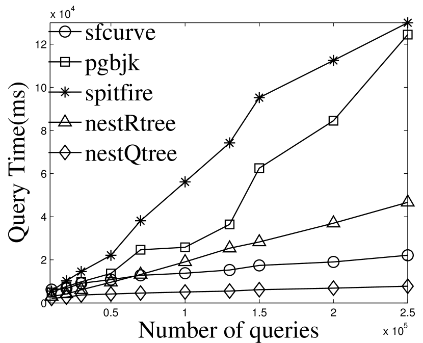
Figure 5(a) gives the performance of the specialized NN join approaches within a local computation node when varying from 10 to 150. The nestQtree approach always performs the best, followed by nestRtree, sfcurve, pgbjk, and spitfire. Notice that block-based approaches induce extensive amounts of NN candidates for query points in the same block, and it directly degrades the performance of the NN refine step. More importantly, the min-distance bound between the MBR of the query points and the MBR of the data points is much smaller than the max-distance boundary. Then, most of the data blocks cannot be pruned, and result in redundant computations. In contrast, the nested-loops join algorithms prune some data blocks because the min-distance bound from the query point to the data points of the same block is bigger than the max-distance boundary of this query point. Figure 5(b) gives the performance of the NN join algorithms by varying the number of query points. Initially, for less than 70k query points, nestRtree outperforms sfcurve, then nestRtree degrades linearly with more query points. Overall, we adopt nestQtree as the NN join algorithm for local workers.

5 Spatial bitmap filter
In this section, we introduce a new spatial bitmap filter termed sFilter. The sFilter helps us decide for an outer tuple, say , of a spatial range join, if there exist tuples in the inner table that actually join with . This helps reduce the communication overhead. For example, consider an outer tuple of a spatial range join where has a range that overlaps multiple data partitions of the inner table. Typically, all the overlapping partitions need to be examined by communicating ’s range to them, and searching the data within each partition to test for overlap with ’s range. This incurs high communication and search costs. Using the sFilter, given ’s range that overlaps multiple partitions of the inner table, the sFilter can decide which overlapping partitions contain data that overlaps ’s range without actually communicating with and searching the data in the partitions. Only the partitions that contain data that overlap with ’s range are the ones that will be contacted and searched.
5.1 Overview of the sFilter
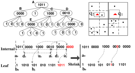
Figure 6 gives an example of an sFilter. Conceptually, an sFilter is a new in-memory variant of a quadtree that has internal and leaf nodes [18]. Internal nodes are for index navigation, and leaf nodes, each has a marker to indicate whether or not there are data items in the node’s corresponding region. We encode the sFilter into two binary codes and execute queries over this encoding.
5.1.1 Binary Encoding of the sFilter
The sFilter is encoded into two long sequences of bits. The first bit-sequence corresponds to internal nodes while the second bit-sequence corresponds to leaf nodes. Notice that in these two binary sequences, no pointers are needed. Each internal node of the sFilter takes four bits, where each bit represents one of the internal node’s children. These children are encoded in clock-wise order starting from the upper-left corner. Each bit value of an internal node determines the type of its corresponding child, i.e., whether the child is internal (a 1 bit) or leaf (a 0 bit). In Figure 6, the root (internal) node has binary code , i.e., it has three of its children being internal nodes, and its second node is leaf. The four-bit encodings of all the internal nodes are concatenated to form the internal-node bit-sequence of the sFilter. The ordering of the internal nodes in this sequence is based on a breadth-first search (BFS) traversal of the quadtree. In contrast, a leaf node only takes one bit, and its bit value indicates whether or not data points exist inside the spatial quadrant corresponding to the leaf. In Figure 6, internal node has four children, and the bit values for ’s leaf nodes are , i.e., the first and third leaf nodes of contain data items. During the BFS on the underlying quad-tree of the sFilter, simultaneously construct the bit-sequences for all the leaf and internal nodes. The sFilter is encoded into the two binary sequences in Figure 6. The space usage of an sFilter is Bits, where and are the numbers of internal nodes and leaf nodes, respectively, and is the depth of quadtree and is the length of the space.
5.1.2 Query Processing Using the sFilter
Consider the internal node in Figure 6. ’s binary code is , and the third bit has a value of 1 at memory address of the internal nodes bit sequence. Thus, this bit refers to ’s child that is also an internal node at address . Because the sFilter has no pointers, we need to compute ’s address from . Observe that the number of bits with value 1 from the start address of the binary code to can be used to compute the address.
Definition 6
Let be the bit sequence that starts at address . and are the number of bits with value 1 and 0, respectively, from addresses to inclusive.
is the number of internal nodes up to . Thus, the address of is because there are 5 bits with value 1 from to . Similarly, if one child node is a leaf node, its address is inferred from as follows:
Proposition 1
Let and be the sFilter’s bit sequences for internal and leaf nodes in memory addresses and , respectively. To access a node’s child in memory, we need to compute its address. The address, say , of the th child of an internal node at address is computed as follows. If the bit value of is 1, then . If the bit value of is 0, .
We adopt the following two optimizations to speedup the computation of and : (1) Precomputation and (2) Set counting. Let be the memory address of the first internal node at height (or depth) of the underlying quadtree when traversed in BFS order. For example, in Figure 6, nodes and are the first internal nodes in BFS order at depths 1 and 2 of the quadtree, respectively. For all depth of the underlying quadtree, we precompute , e.g., and in Figure 6. Notice that and . Then, address that corresponds to the memory address of the th child of an internal node at address can be computed as follows. . is precomputed. Thus, we only need to compute on the fly . Furthermore, evaluating can be optimized by a bit set counting approach, i.e, a lookup table or a sideways addition 111https://graphics.stanford.edu/~seander/bithacks.html that can achieve constant time complexity.
After getting one node’s children via Proposition 1, we apply Depth-First Search (DFS) over the binary codes of the internal nodes to answer a spatial range query. The procedure starts from the first four bits of bit sequence , since these four bits are the root node of the sFilter. Then, we check the four quadrants, say , of the children of the root node, and iterate over to find the quadrants, say , overlapping the input query range . Next, we continue searching the children of based on the addresses computed from Proposition 1. This recursive procedure stops if a leaf node is found with value 1, or if all internal nodes are visited. For example, consider range query in Figure 6. We start at the root node (with bit value ). Query is located inside the northwestern (NW) quadrant of . Because the related bit value for this quadrant is 1, it indicates an internal node type and it refers to child node . Node ’s memory address is computed by because only one non-leaf node () is before . ’s related bit value is , i.e., contains four leaf nodes. The procedure continues until finding one leaf node of , mainly the southeastern child leaf node, with value 1 that overlaps the query, and thus returns true.
5.2 sFilter in LocationSpark
Since the depth of the sFilter affects query performance, it is impractical to use only one sFilter in a distributed setting. We thus embed multiple sFilters into the global and local spatial indexes in LocationSpark. In the master node, separate sFilters are placed into the different branches of the global index, where the role of each sFilter is to locally answer the query for the specific branch it is in. In the local computation nodes, an sFilter is built and it adapts its structure based on data updates and changes in query patterns.
5.2.1 Spatial Query Processing Using the sFilter
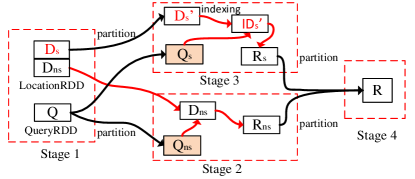
Algorithm 2 gives the procedure for performing the spatial range join using the sFilter. Initially, the outer (queries) table is partitioned according to the global index. The global index identifies the overlapping data partitions for each query . Then, the sFilter tells which partitions contain data that overlap the query range (Line 2 of the algorithm). After performing the spatial range join (Line 14), the master node fetches the updated sFilter from each data worker, and refreshes the existing sFilters in the master node (Lines 15-16). Lines 2-13 update the sFilter of each worker (as in Figure 2).
The sFilter can improve the NN search and NN join because they also depend on spatial range search. Moreover, their query results may enhance the sFilter by lowering the false positive errors as illustrated below.
5.2.2 Query-aware Adaptivity of the sFilter
The build and update operations of the sFilter are first executed at the local workers in parallel. Then, the updated sFilters are propagated to the master node.
The initial sFilter is built from a temporary local quadtree [18] in each partition. Then, the sFilter is adapted based on the query results. For example, consider Query in Figure 6. Initially, the sFilter reports that there is data for in the partitions. When visits the related data partitions, it finds that there are actually no data points overlapping with in the partitions, i.e., a false-positive (+ve) error. Thus, we mark the quadrants precisely covered by in the sFilter as empty, and hence reduce the false positive errors if queries visit the marked quadrants again. Function insert in Algorithm 2 recursively splits the quadrants covered by the empty query, and marks these generated quadrants as empty. After each local sFilter is updated in each worker, these updates are reflected into the master node. The compact encoding of the sFilter saves the communication cost between the workers and the master.
However, the query performance of the sFilter degrades as the size of the index increases. Function shrink in Algorithm 2 merges some branches of the sFilter at the price of increasing false +ve errors. For example, one can shrink internal node in Figure 6 into a leaf node, and updating its bit value to 1, although one quadrant of does not contain data. Therefore, we might track the visit frequencies of the internal nodes, and merge internal nodes with low visiting frequency. Then, some well-known data caching policies, e.g., LRU or MRU, can be used. However, the overhead to track the visit frequencies is expensive. In our implementation, we adopt a simple bottom-up approach. We start merging the nodes from the lower levels of the index to the higher levels until the space constraint is met. In Figure 6, we shrink the sFilter from internal node , and replace it by a leaf node, and update its binary code to . ’s leaf children are removed. The experimental results show that this approach increases the false +ve errors, but enhances the overall query performance.
6 Performance Study
LocationSpark is implemented on top of Resilient Distributed Datasets (RDDs); these key components of Spark are fault-tolerant collections of elements that can be operated on in parallel. LocationSpark is a library of Spark and provides the Class LocationRDD for spatial operations [16]. Statistics are maintained at the driver program of Spark, and the execution plans are generated at the driver. Local spatial indexes are persisted in the RDD data partitions, while the global index is realized by extending the interface of the RDD data partitioner. The data tuples and related spatial indexes are encapsulated into the RDD data partitions. Thus, Spark’s fault tolerance naturally applies in LocationSpark. The spatial indexes are immutable and are implemented based on the path copy approaches. Thus, each updated version of the spatial index can be persisted into disk for fault tolerance. This enables the recovery of a local index from disk in case of failure in a worker. The Spark cluster is managed by YARN, and a failure in the master nodes is detected and managed by ZooKeeper. In case of master node failure, the lost master node is evicted and a standby node is chosen to recover the master. As a result, the global index and the sFilter in the master node are recoverable. Finally, the built spatial index data can be stored into disk, and enable further data analysis without additional data repartitioning or indexing. LocationSpark is open-source, and can be downloaded from https://github.com/merlintang/SpatialSpark.
6.1 Experimental Setup
Experiments are conducted on two datasets. Twitter: 1.5 Billion Tweets (around 250GB) are collected over a period of nearly 20 months (from January 2013 to July 2014) and is restricted to the USA spatial region. The format of a tweet is: identifier, timestamp, longitude-latitude coordinates, and text. OSMP: is shared by the authors of SpatialHadoop [9]. OSMP represents the map features of the whole world, where each spatial object is identified by its coordinates (longitude, latitude) and an object ID. It contains 1.7 Billion points with a total size of 62.3GB. We generate two types of queries. (1) Uniformly distributed (USA, for short): We uniformly sample data points from the corresponding dataset and generate spatial queries from the samples. These are the default queries in our experiments. (2) Skewed spatial queries: These are synthesized around specific spatial areas, e.g., Chicago, San Francisco, New York (CHI, SF, NY, correspondingly, for short). The spatial queries and data points are the outer table and the inner table for the experimental studies of the spatial range and NN joins presented below.
Our study compares LocationSpark with the following: (1) GeoSpark [25] uses ideas from SpatialHadoop but is implemented over Spark. (2) SpatialSpark [2] performs partition-based spatial joins. (3) Magellan [1] is developed based on Spark’s dataframes to take advantage from Spark SQL’s plan optimizer. However, Magellan does not have spatial indexing. (4) State-of-art NN-join: Since none of the three systems support NN join, we compare LocationSpark with a state-of-art NN-join approach (PGBJ [15]) that is provided by PGBJ’s authors. (5) Simba [24] is a spatial computation system based on Spark SQL with spatial distance join and NN-join operator. We also modified Simba with the developed techniques (e.g., query scheduler and sFilter) inside, the optimized Simba is called Simba(opt). (6) LocationSpark(opt) and LocationSpark refers to the query scheduler and sFilter is applied or not, respectively.
We use a cluster of six physical nodes Hathi 222https://www.rcac.purdue.edu/compute/hathi/. that consists of Dell compute nodes with two 8-core Intel E5-2650v2 CPUs, 32 GB of memory, and 48TB of local storage per node. Meanwhile, in order to test the scalability of system, we setup one Hadoop cluster (with Hortonworks data paltform 2.5) on the the Amazon EC2 with 48 nodes, each node has an Intel Xeon E5-2666 v3 (Haswell) and 8GB of memory. Spark 1.6.3 is used with YARN cluster resource management. Performance is measured by the average query execution time.
| Dataset | System | Query time(ms) | Index build time(s) |
|---|---|---|---|
| LocationSpark(R-tree) | 390 | 32 | |
| LocationSpark(Qtree) | 301 | 16 | |
| Magellan | 15093 | / | |
| SpatialSpark | 16874 | 35 | |
| SpatialSpark(no-index) | 14741 | / | |
| GeoSpark | 4321 | 45 | |
| Simba | 1231 | 34 | |
| Simba (opt) | 430 | 35 | |
| OSMP | LocationSpark(R-tree) | 1212 | 67 |
| LocationSpark(Qtree) | 734 | 18 | |
| Magellan | 41291 | / | |
| SpatialSpark | 24189 | 64 | |
| SpatialSpark(no-index) | 17210 | / | |
| GeoSpark | 4781 | 87 | |
| Simba | 1345 | 68 | |
| Simba(opt) | 876 | 68 |
6.2 Spatial Range Search and Join
Table I summarizes the spatial range search and spatial index build time by the various approaches. For a fair comparison, we cache the indexed data into memory, and record the spatial range query processing time. From Table I, we observe the following: (1) LocationSpark is 50 times better than Magellan on query execution time for the two tables, mainly because the spatial index (e.g., Global and Local index) of LocationSpark can avoid visiting unnecessary data partitions. (2) LocationSpark with different local indexes, e.g., the R-tree and Quadtree, outperforms SpatialSpark. The speedup is around 50 times, since SpatialSpark (without index) has to scan all the data partitions. SpatialSpark (with index) stores the global indexes into disk, and finds data partitions by scanning the global index in disk. This incurs extra I/O overhead. Also, the local index is not utilized during local searching. (3) LocationSpark is around 10 times faster than GeoSpark in spatial range search execution time because GeoSpark does not utilize the built global indexes and scans all data partitions. (4) The local index with Quadtree for LocationSpark achieves superior performance over the R-tree one in term of index construction and query execution time as discussed in Section 4. (5) The index build time among the three systems is comparable because they all scan the data points, which is the dominant factor, and then build the index in memory. (6) LocationSpark achieve 5 times speedup against with Simba, since sFilter can reduce redundant data partitions searching. This is also observed from the Simba(opt) (i.e., with sFilter) can achieve comparable performance with LocationSpark.
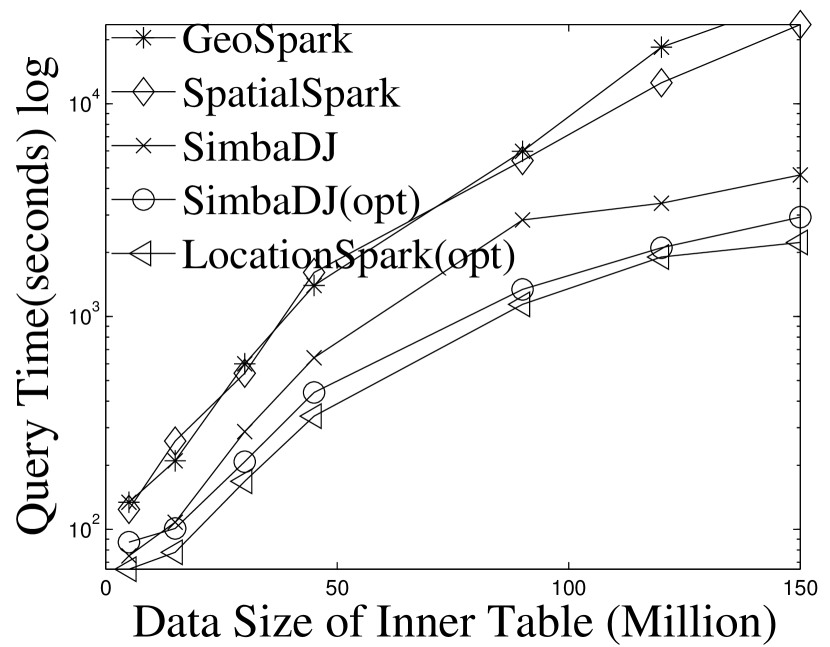
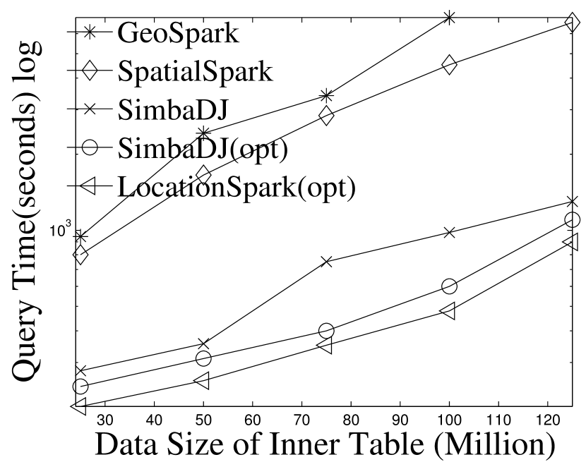
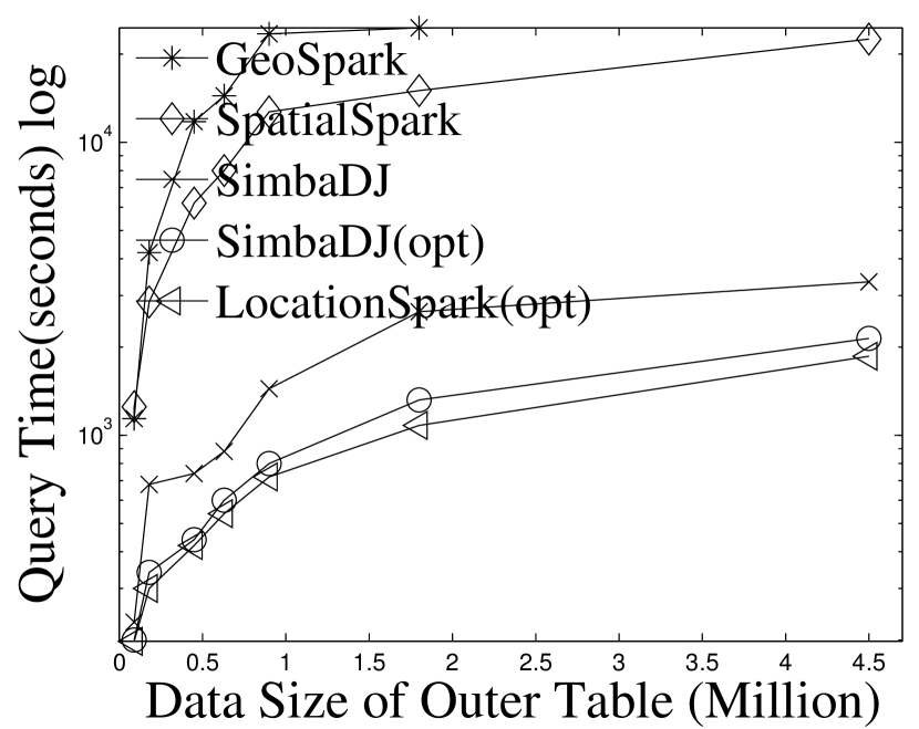
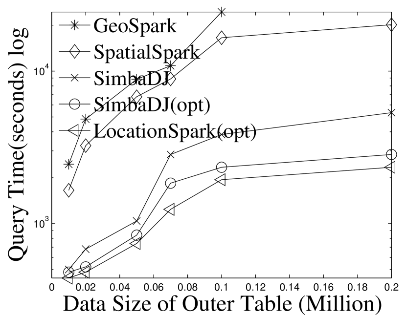
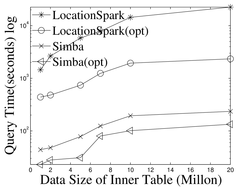
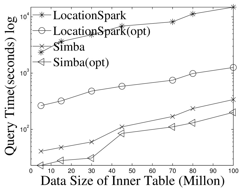
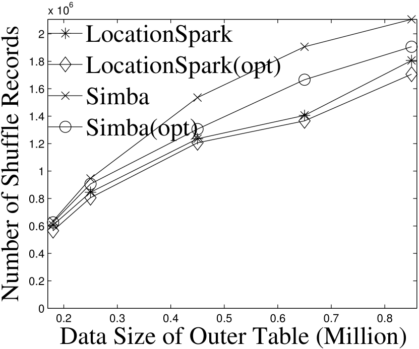
Performance results (mainly, the execution times of the spatial range join) are listed in Figure 7. For fair comparison, the runtime includes the time to initiate the job, build indexes, execute the join query, and save results into HDFS. Note that Simba does not support spatial range join, it only provides the spatial distance join, where each query is rectangle or circle with the same size. Performance results for Magellan are not shown because it performs a Cartesian product and hence has the worst execution time. Figures 7(a) and 7(b) present the results by varying the data sizes of (the inner table) from 25 million to 150 million, while keeping the size of (the outer table) to 0.5 million. The execution time of GeoSpark shows quadratic increase as the data size increases. GeoSpark’s running time is almost 3 hrs when the data size is 150 million, which is extremely slow. SpatialSpark shows similar trends. The reason is that both GeoSpark and SpatialSpark suffer from (1) the spatial skew issue where some workers process more data and take longer time to finish. (2) the local execution plan based on the R-tree and the Grid is slow. (3) processing of queries go to data partitions that do not contribute to the final results. LocationSpark with the optimized query plans and the sFilter outperforms the two other systems by an order of magnitude. Also, we study the effect of the outer table size on performance. Figures 7(c) and 7(d) give the run time, and demonstrate that LocationSpark is 10 times faster than the other two systems. From Figure 7, we also observe Simba outperform GeoSpark and SpatialSpark more than one order of magnitude, however, Simba also suffer from the query skew issues and degrade the performance quickly, because Simba has to duplicate each data point into multiple data partitions if its spatial overlapping with query rectangles. Naturally, the bigger spatial query rectangle, the more data points to be duplicated. This brings redundant network and computation costs. Thus, we place the query scheduler and sFilter into the physical execution part of Simba (e.g., modifying the RDKspark). From the experimental result, the performance of Simba is improved dramatically. This also proves the proposed approaches in this work could be used for improve most in-memory distributed spatial query processing systems.
6.3 Performance of kNN Search and Join
Performance of NN search is listed in Table II. LocationSpark outperforms GeoSpark by an order of magnitude. GeoSpark broadcasts the query points to each data partition, and accesses each data partition to get the NN set for the query. Then, GeoSpark collects the local results from each partition, then sorts the tuples based on the distance to query point of NN. This is prohibitively expensive, and results in large execution time. LocationSpark only searches for data partitions that contribute to the NN query point based on the global and local spatial indexes and the sFilter. It avoids redundant computations and unnecessary network communication for irrelevant data partitions.
For NN join, Table III presents the performance results when varying on the Twitter and OSMP datasets. In terms of runtime, LocationSpark with optimized query plans and with the sFilter always performs the best. LocationSpark without any optimizations gives better performance than that of PGBJ. The reason is due to having in-memory computations and avoiding expensive disk I/O when compared to MapReduce jobs. Furthermore, LocationSpark with optimization shows around 10 times speedup over PGBJ, because the optimized plan migrates and splits the skewed query regions.
We test the performance of the NN join operator when increasing the number of data points while having the number of queries fixed to 1 million around the Chicago area. The results are illustrated in Figure 8. Observe that LocationSpark with optimizations performs an order of magnitude better than the basic approach. The reason is that the optimized query plan identifies and repartitions the skewed partitions. In this experiment, the top five slowest tasks in LocationSpark without optimization take around 33 minutes, while more than 75% tasks only take less than 30 seconds. On the other hand, with an optimized query plan, the top five slowest tasks take less than 4 minutes. This directly enhances the execution time.
More interesting, we observe Simba outperforms LocationSpark around 10 times for the NN join operation. This speedup is achieved by implementing the NN join via a sampling technique in Simba. More specifically, Simba at first samples certain amount of query points and computes the NN join bound, s.t. pruning data partitions which do not contribute NN join results. The computed NN bound could be very tight when the is small and query points are balanced distributed. More details can be found in the Section 6.3.3 of Simba. However, the computed NN join bound have to do spatial overlapping checking with data points, then duplicate query points to the overlapping data partitions as well. As a result, Simba would suffer from the query skew where certain data partitions are overwhelmed with query points. Furthermore, the bigger also brings redundant network communication because the NN join bound would be bigger as well. Similar as spatial join, we placed spatial query scheduler and sFilter inside the physical execution part of Simba. The query scheduler can detect the skew data partitions, as well as sFilter to remove data partitions which overlapping with NN join bound but fail to contribute final result. Therefore, the performance of Simba is further improved, e.g., more than three times in this experimental setting.
| Dataset | System | k=10 | k=20 | k=30 |
|---|---|---|---|---|
| LocationSpark(R-tree) | 81 | 82 | 83 | |
| LocationSpark(Q-tree) | 74 | 75 | 74 | |
| GeoSpark | 1334 | 1813 | 1821 | |
| Simba | 420 | 430 | 440 | |
| Simba(opt) | 80 | 83 | 87 | |
| OSMP | LocationSpark(R-tree) | 183 | 184 | 184 |
| LocationSpark(Q-tree) | 73 | 73 | 74 | |
| GeoSpark | 4781 | 4947 | 4984 | |
| Simba | 330 | 340 | 356 | |
| Simba(opt) | 167 | 186 | 190 |
| Dataset | System | k=50 | k=100 | k=150 |
|---|---|---|---|---|
| LocationSpark(Q-tree) | 340 | 745 | 1231 | |
| LocationSpark(Opt) | 165 | 220 | 230 | |
| PGBJ | 3422 | 3549 | 3544 | |
| Simba | 40 | 44 | 48 | |
| Simba(Opt) | 21 | 22 | 31 | |
| OSMP | LocationSpark(Q-tree) | 547 | 1241 | 1544 |
| LocationSpark(Opt) | 260 | 300 | 340 | |
| PGBJ | 5588 | 5612 | 5668 | |
| Simba | 51 | 55 | 61 | |
| Simba(Opt) | 23 | 26 | 28 |
6.4 Effect of Query Distribution
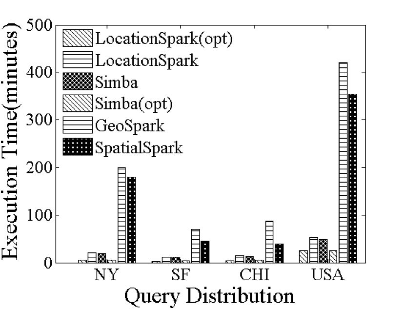
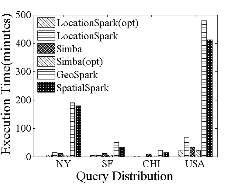
We study the performance under various query distributions. As illustrated before, the query execution plan is the most effective factor in distributed spatial computing. From the experimental results for spatial range join and NN join above, we already observe that the system with optimization achieves much better performance over the unoptimized versions. In this experiment, we study the performance of the optimized query scheduling plan in LocationSpark under various query distributions. The performance of the spatial range join operator over query set (the outer table) and dataset (the inner table) is used as the benchmark. The number of tuples for is fixed as 15 million and 50 million for Twitter and OSMP, respectively, while the size of is 0.5 million, and each query in is generated from different spatial regions, e.g., CHI, SF, NY and USA. We do not plot the runtime of Magellan on spatial join, as it uses Cartesian join, and hence has the worst performance. Figure 9 gives the execution runtimes for the spatial range join operators in different spatial regions. From Figure 9, GeoSpark performs the worst, followed by SpatialSpark and then LocationSpark. LocationSpark and Simba(opt) with the optimized query plan achieves an order of magnitude speedup over GeoSpark and SpatialSpark in terms of execution time. LocationSpark with optimized plans achieves more than 10 times speedup over LocationSpark without the optimized plans for the skewed spatial queries. Meanwhile, Simba could be further improved more than five times comparing with system without optimization.
6.5 Effect of the sFilter
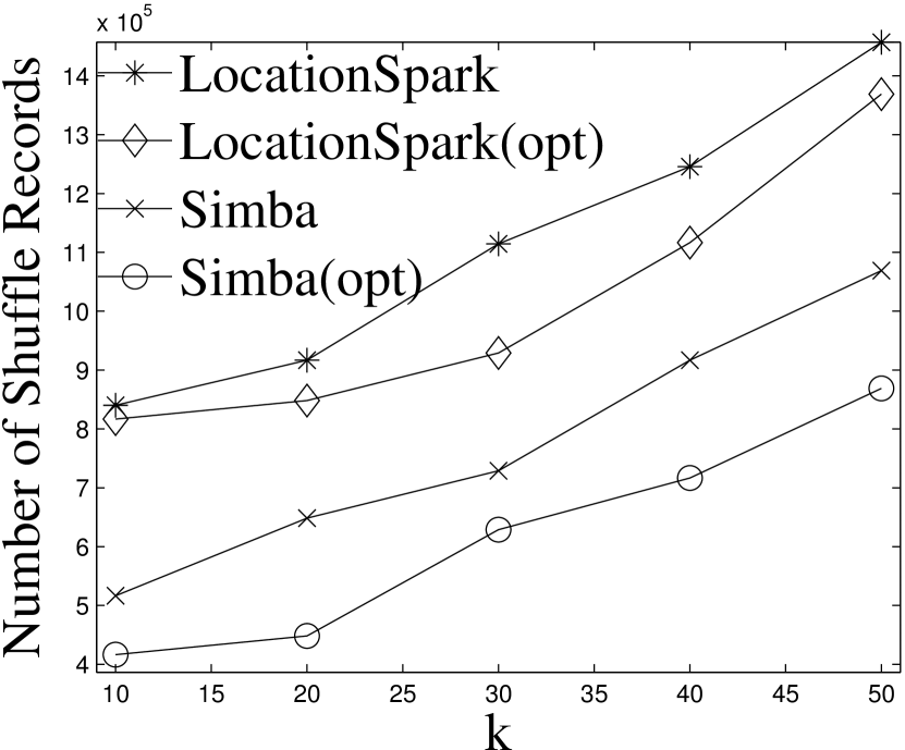
In this experiment, we measure the spatial range query processing time, the index construction time, the false positive ratio and the space usage of the sFilter on a single machine. Table IV gives the performance of various indexes in a local computation node. The Bloom filter is tested using breeze 333https://github.com/scalanlp/breeze. The sFilter(ad) represents the sFilter with adaptation of its structure given changes in the queries, and with the merging to reduce its size as introduced in Section 5.2.2. From Table IV, observe that sFilter achieves one and two orders of magnitude speedup over the Quadtree- and R-tree-based approaches in terms of spatial range search execution time, respectively. The sFilter(ad) improves the query processing time over the approach without optimization, but the sFilter(ad) has the overhead to merge branches of the index to control its size, and increases the false positive ratio. The Bloom filter does not support spatial range queries. Table IV also gives the space usage overhead for various local indexes in each worker. The sFilter is 5-6 orders of magnitude less than the other types of indexes, e.g., the R-tree and the Quadtree. This is due to the bit encoding of the sFilter that eliminates the need for pointers. Moreover, the sFilter reduces the unnecessary network communication. We study the shuffle cost for redistributing the queries. The results are given in Figure 10. The sFilter reduces the shuffling cost for both spatial range and NN join operations. The shuffle cost reduction depends on the data and query distribution. Thus, the more unbalanced the distribution of queries and data in the various computation nodes, the more shuffle cost is reduced. For example, for NN join based on LocationSpark, the shuffle cost is improved from 1114575 to 928933 when is 30, achieving 18% reduction in network communication cost. The sFilter also reduce the network communication cost for Simba
| Dataset | Index | Query time(ms) | Index build(s) | False positive | Memory usage(MB) |
|---|---|---|---|---|---|
| R-tree | 19 | 17 | / | 112 | |
| Q-tree | 0.4 | 1.8 | / | 37 | |
| sFilter | 0.022 | 2 | 0.07 | 0.006 | |
| sFilter(ad) | 0.018 | 2.3 | 0.09 | 0.003 | |
| Bloom filter | 0.004 | 1.54 | 0.01 | 140 | |
| OSMP | R-tree | 4 | 32 | / | 170 |
| Q-tree | 0.5 | 1.2 | / | 63 | |
| sFilter | 0.008 | 2.4 | 0.06 | 0.008 | |
| sFilter(ad) | 0.006 | 6 | 0.10 | 0.006 | |
| Bloom filter | 0.002 | 2.7 | 0.01 | 180 |
6.6 Effect of the Number of Workers
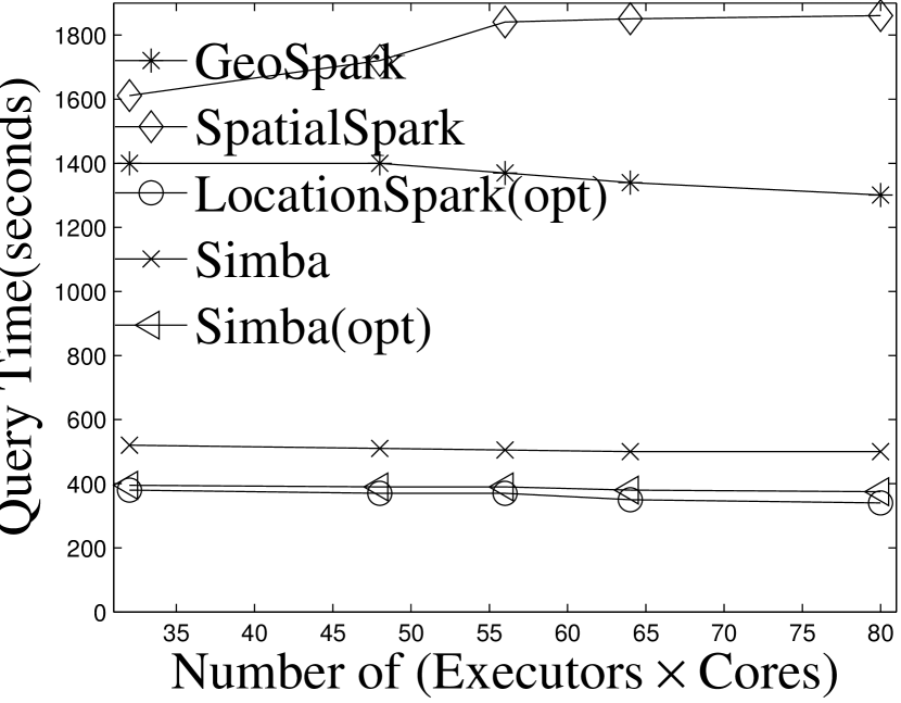
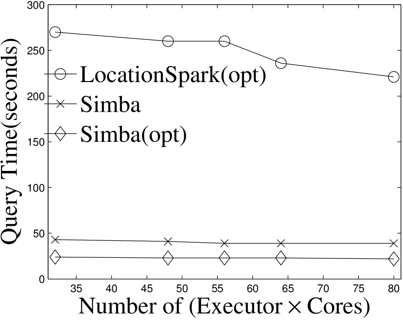
Spark’s parallel computation ability depends on the number of executors and number of CPU cores assigned to each executor, that is, the number of executors times the number of CPU cores per executor. Therefore, to demonstrate the scalability of the proposed approach, we change the number of executors from 4 to 10, and fix the number of CPU cores assigned to each executor. We study the runtime performance for spatial range join and NN join operations using the Twitter and OSMP datasets on the Amazon EC2 cluster. Because the corresponding performance on the OSMP dataset gives similar trends as the Twitter dataset, we only present the performance for the Twitter dataset in Figure 11, where the outer table size is fixed to 1 million around Chicago area, and the inner table size is 15 million. We observe that the performance of LocationSpark and Simba(opt) for the spatial range join and the NN join improves gradually with the increase in the number of executors. In contrast, GeoSpark and SpatialSpark do not scale well in comparison to LocationSpark for spatial range join. The performance of Magellan for spatial join is not shown because it is based on Cartesian product and shows the worst performance.
7 Related Work
Spatial data management has been extensively studied for decades and several surveys provide good overviews. Gaede and Günther [10] provide a good summary of spatial data indexing. Sowell et al. give a survey and experimental study of iterative spatial-join in memory [20]. Recently, there has been considerable interest in supporting spatial data management over Hadoop MapReduce. Hadoop-GIS [3] supports spatial queries in Hadoop by using a uniform grid index. SpatialHadoop [9] builds global and local spatial indexes, and modifies the HDFS record reader to read data more efficiently. MD-Hbase [17] extends HBase to support spatial data update and queries. Hadoop MapReduce is good at data processing for high throughput and fault-tolerance.
Taking advantage of the very large memory pools available in modern machines, Spark and Spark-related systems (e.g., Graphx, Spark-SQL, and DStream) [12, 26] are developed to overcome the drawbacks of MapReduce in specific application domains. In order to process big spatial data more efficiently, it is natural to develop an efficient spatial data management systems based on Spark. Several prototypes have been proposed to support spatial operations over Spark, e.g., GeoSpark [25], SpatialSpark [2], Magellan [1], Simba [24]. However, some important factors impede the performance of these systems, mainly, query skew, lack of adaptivity, and excessive and unoptimized network and I/O communication overheads. For existing spatial join [20, 6] and NN join approaches [23, 8, 15], we conduct experiments to study their performance in Section 4. The reader is referred to Section 4. For testing how the proposed techniques to improve Simba, we placed the spatial query scheduler ans sFilter into Simba standlone version. The Simba standlone version is based on Spark SQL Dataframe while removing the support of Spark SQL parser. The query scheduler and sFilter is placed into the physical plan of Simba (e.g., RDJSpark and RKJSpark).
Kwon et al. [14, 13] propose a skew handler to address the computation skew in a MapReduce platform. AQWA [5] is a disk-based approach that handles spatial computation skew in MapReduce. In LocationSpark, we overcome the spatial query skew for spatial range join and NN join operators, and provide an optimized query execution plan. These operators are not addressed in AQWA. The query planner in LocationSpark is different from relational query planners, i.e., join order and selection estimation. ARF [4] supports one dimensional range query filter for data in disk. Calderoni et al. [7] study spatial Bloom filter for private data. Yet, it does not support spatial range querying.
8 Conclusions
We presented a query executor and optimizer to improve the query execution plan generated for spatial queries. We introduce a new spatial bitmap filter to reduce the redundant network communication cost. Empirical studies on various real datasets demonstrate the superiority of our approaches compared with existing systems.
9 Acknowledgement
This work is supported by the National Science Foundation under Grant Number III- 1815796.
References
- [1] Magellan. https://github.com/harsha2010/magellan.
- [2] Spatialspark. http://simin.me/projects/spatialspark/.
- [3] A. Aji, F. Wang, H. Vo, R. Lee, Q. Liu, X. Zhang, and J. Saltz. Hadoop gis: A high performance spatial data warehousing system over mapreduce. VLDB, 2013.
- [4] K. Alexiou, D. Kossmann, and P.-A. Larson. Adaptive range filters for cold data: Avoiding trips to siberia. In VLDB, 2013.
- [5] A. M. Aly, A. R. Mahmood, M. S. Hassan, W. G. Aref, M. Ouzzani, H. Elmeleegy, and T. Qadah. AQWA: adaptive query-workload-aware partitioning of big spatial data. In VLDB, 2015.
- [6] T. Brinkhoff, H.-P. Kriegel, and B. Seeger. Efficient processing of spatial joins using r-trees. SIGMOD Rec., 1993.
- [7] L. Calderoni, P. Palmieri, and D. Maio. Location privacy without mutual trust. Comput. Commun.
- [8] G. Chatzimilioudis, C. Costa, D. Zeinalipour-Yazti, W. Lee, and E. Pitoura. Distributed in-memory processing of all k nearest neighbor queries. TKDE, 2016.
- [9] A. Eldawy and M. Mokbel. Spatialhadoop: A mapreduce framework for spatial data. In ICDE, 2015.
- [10] V. Gaede and O. Günther. Multidimensional access methods. ACM Comput. Surv., 30:170–231, 1998.
- [11] M. R. Garey and D. S. Johnson. Computers and Intractability: A Guide to the Theory of NP-Completeness. W. H. Freeman & Co., New York, NY, USA, 1979.
- [12] J. E. Gonzalez, R. S. Xin, A. Dave, D. Crankshaw, M. J. Franklin, and I. Stoica. Graphx: Graph processing in a distributed dataflow framework. In OSDI, 2014.
- [13] Y. Kwon, M. Balazinska, B. Howe, and J. Rolia. Skew-resistant parallel processing of feature-extracting scientific user-defined functions. In SoCC, 2010.
- [14] Y. Kwon, M. Balazinska, B. Howe, and J. Rolia. Skewtune: Mitigating skew in mapreduce applications. In SIGMOD, 2012.
- [15] W. Lu, Y. Shen, S. Chen, and B. C. Ooi. Efficient processing of k nearest neighbor joins using mapreduce. Proc. VLDB Endow., 2012.
- [16] T. Mingjie, Y. Yongyang, G. A. Walid, M. M. Qutaibah, O. Mourad, and R. Ahmed. Locationspark: A distributed in-memory data management system for big spatial data. Purdue technical report, 2016.
- [17] S. Nishimura, S. Das, D. Agrawal, and A. Abbadi. Md-hbase: A scalable multi-dimensional data infrastructure for location aware services. In MDM 11.
- [18] H. Samet. Foundations of Multidimensional and Metric Data Structures. Morgan Kaufmann Publishers Inc., 2005.
- [19] K. Shvachko, H. Kuang, S. Radia, and R. Chansler. The hadoop distributed file system. In MSST, 2010.
- [20] B. Sowell, M. V. Salles, T. Cao, A. Demers, and J. Gehrke. An experimental analysis of iterated spatial joins in main memory. Proc. VLDB Endow., 2013.
- [21] M. Tang, Y. Yu, W. G. Aref, Q. Malluhi, and M. Ouzzani. Locationspark: A distributed in-memory data management system for big spatial data. VLDB, 2016.
- [22] J. S. Vitter. Random sampling with a reservoir. ACM Trans. Math. Softw., 1985.
- [23] C. Xia, H. Lu, B. Chin, and O. J. Hu. Gorder: An efficient method for knn join processing. In VLDB, 2004.
- [24] D. Xie, F. Li, B. Yao, G. Li, L. Zhou, and M. Guo. Simba: Efficient in-memory spatial analytics. In SIGMOD, 2016.
- [25] J. Yu, J. Wu, and M. Sarwat. Geospark: A cluster computing framework for processing large-scale spatial data. In SIGSPATIAL, 2015.
- [26] M. Zaharia. An Architecture for Fast and General Data Processing on Large Clusters. Association for Computing Machinery and Morgan, 2016.
| Mingjie Tang is member of technical stuff at Hortonworks. He won his PhD at Purdue University. His research interests include database system and big data infrastructure. He has an MS in computer science from the University of Chinese Academy of Sciences, BS degree from Sichuan University, China. |
| Yongyang Yu is a PhD student at Purdue University. His research focus is on big data management and matrix computation. |
| Walid G. Aref is a professor of computer science at Purdue. He is an associate editor of the ACM Transactions of Database Systems (ACM TODS) and has been an editor of the VLDB Journal. He is a senior member of the IEEE, and a member of the ACM. Professor Aref is an executive committee member and the past chair of the ACM Special Interest Group on Spatial Information (SIGSPATIAL). |
| Ahmed R.Mahmood is a PhD student at Purdue University. His research focus is on big spatial-keyword data management. |
| Qutaibah M. Malluhi joined Qatar University in September 2005. He is the Director of the KINDI Lab for Computing Research. He served as the head of Computer Science and Engineering Department at Qatar University between 2005-2012. |
| Mourad Ouzzani is a Principal Scientist with the Qatar Computing Research Institute (QCRI), Qatar Foundation. He is interested in research and development related to data management and scientific data and how they enable discovery and innovation in science and engineering. Mourad received the Purdue University Seeds of Success Award in 2009 and 2012. |
.1 Proof of data repartition and query plan optimization problem
Proof:
We prove it by reduction from the Bin-Packing problem [11]. Bin-Packing is defined as giving the finite set of items, the size of each item, says , is a positive real number, while , and a positive integer bin capacity , and a positive Integer , we want to find a partition of into disjoint set such that the sum of the size of items in each is or less. Let be the solution to the reduced optimal data repartition problem. Next we show that based on , we can obtain the solution to the original Bin-Packing problem in polynomial time.
To reduce this Bin-Packing problem to optimal data repartition problem, we first assume the skew and non-skew set is known. In practical, we can sort data partitions based on their approximate runtime , and then find skewed partitions based on certain threshold. This takes polynomial time. Then the runtime over non-skewed partition is , and is a constant value. Meanwhile, we disregard the minimization condition over . Therefore, from Equation 5, we can simplify this data repartition problem as
| (7) |
From this formula, we can find is a constant value, thus, we have to minimize our cost function to be smaller than , that is,
| (8) |
| (9) |
To simplify this function further, we disregard the optimization over , we can simply our problem as following
| (10) |
Suppose the total number of new generated data partition is , this function is written as this way.
| (11) |
Therefore, if , when , we can make sure our optimal function is at least less than its upper bound.
In addition, we assume that optimizer could split the skew data partitions into partitions and , and each new computed data partition is associated with the cost . Now, optimizer can pack the computed partitions into a disjoint set, s.t., (1) the size of disjoint set is , because is maximum number of data partitions. (2) the sum of cost in each bin would be smaller than based on Equation 11. From this way, we can find this is same as the Bin-Packing problem. Thus, if is the solution of the optimal data repartition problem, then, we can use to compute the solution for the Bin-Packing problem. Since Bin-Packing is known to be NP-complete, and Bin-Packing is easier than optimal data repartition problem, we can deduce that optimal data repartition problem is also NP-complete. ∎