Robust Guarantees for Perception-Based Control

Abstract

Motivated by vision-based control of autonomous vehicles, we consider the problem of controlling a known linear dynamical system for which partial state information, such as vehicle position, is extracted from complex and nonlinear data, such as a camera image. Our approach is to use a learned perception map that predicts some linear function of the state and to design a corresponding safe set and robust controller for the closed loop system with this sensing scheme. We show that under suitable smoothness assumptions on both the perception map and the generative model relating state to complex and nonlinear data, parameters of the safe set can be learned via appropriately dense sampling of the state space. We then prove that the resulting perception-control loop has favorable generalization properties. We illustrate the usefulness of our approach on a synthetic example and on the self-driving car simulation platform CARLA.

Keywords. Robust control, learning theory, generalization, perception, robotics.

1 Introduction

Incorporating insights from rich, perceptual sensing modalities such as cameras remains a major challenge in controlling complex autonomous systems. While such sensing systems clearly have the potential to convey more information than simple, single output sensor devices, interpreting and robustly acting upon the high-dimensional data streams remains difficult. Recent end-to-end approaches tackle the problem of image based control by learning an optimized map from pixel values directly to low level control inputs. Though there has been tremendous success in accomplishing sophisticated tasks, critical gaps in understanding robustness and safety still remain [38]. On the other hand, methods rooted in classical state estimation and robust control explicitly characterize a model of the underlying system and its environment in order to design a feedback controller. These approaches have provided strong and rigorous guarantees of robustness and safety in domains such as aerospace and process control, but the level of specification of the underlying system required has thus far limited their impact for complex sensor inputs.

In this paper, we aim to leverage contemporary techniques from machine learning and robust control to understand the conditions under which safe and reliable behavior can be achieved in controlling a system with uncertain and high-dimensional sensors. Whereas much recent work has been devoted to proving safety and performance guarantees for learning-based controllers applied to systems with unknown dynamics [65, 5, 47, 32, 22, 23, 2, 1, 16, 63, 68, 4, 12], we focus on the practical scenario where the underlying dynamics of a system are well understood, and it is instead the integration of perceptual sensor data into the control loop that must be learned. Specifically, we consider controlling a known linear dynamical system for which partial state information can only be extracted from complex observations. Our approach is to design a virtual sensor by learning both a perception map (i.e., a map from observations to a linear function of the state) and a bound on its estimation errors. We show that under suitable smoothness assumptions, we can guarantee bounded errors within a neighborhood of the training data. This model of uncertainty allows us to synthesize a robust controller that ensures that the system does not deviate too far from states visited during training. Finally, we show that the resulting perception and robust control loop is able to robustly generalize under adversarial noise models. To the best of our knowledge, this is the first such guarantee for a vision-based control system.

1.1 Related work

Vision based estimation, planning, and control

There is a rich body of work, spanning several research communities, that integrate complex sensing modalities, specifically cameras, into estimation, planning, and control loops. The robotics community has focused mainly on integrating camera measurements with inertial odometry via an Extended Kalman Filter (EKF) [34, 35, 31]. Similar approaches have also been used as part of Simultaneous Localization and Mapping (SLAM) algorithms in both ground  [42] and aerial [41] vehicles. We note that these works focus solely on the estimation component, and do not consider downstream use of state estimates in control loops. In contrast, the papers  [40, 62, 39] demonstrate techniques that use camera measurements to aid inertial position estimates to enable aggressive control maneuvers in unmanned aerial vehicles.

The machine learning community has taken a more data-driven approach. The earliest such example is likely [52], in which a 3-layer neural-network is trained to infer road direction from images. Modern approaches to vision based planning, typically relying on deep neural networks, include learning maps from image to trail direction  [28], learning Q-functions for indoor navigation using 3D CAD images [56], and using images to specify waypoints for indoor robotic navigation [11]. Moving from planning to low-level control, end-to-end learning for vision based control has been achieved through imitation learning from training data generated via human [15] and model predictive control [50]. The resulting policies map raw image data directly to low-level control tasks. In Codevilla et al. [19], higher level navigational commands, images, and other sensor measurements are mapped to control actions via imitation learning. Similarly, Williams et al. [68] and related works, image and inertial data is mapped to a cost landscape, that is then optimized via a path integral based sampling algorithm. More closely related to our approach is Lambert et al. [37], where a deep neural network is used to learn a map from image to system state – we note that this perception module is naturally incorporated into our proposed pipeline. To the best of our knowledge, none of the aforementioned results provide safety or performance guarantees.

Learning, robustness, and control

Our theoretical contributions are similar in spirit to those of the online learning community, in that we provide generalization guarantees under adversarial noise models [6, 7, 36, 30, 70]. Similarly, Agarwal et al. [4] shows that adaptive disturbance feedback control of a linear system under adversarial process noise achieves sublinear regret – we note that this approach assumes full state information. We also draw inspiration from recent work that seeks to bridge the gap between linear control and learning theory. These assume a linear time invariant system, and derive finite-time guarantees for system identification [22, 29, 61, 57, 49, 58, 64, 26, 27, 51], and/or integrate learned models into control schemes with finite-time performance guarantees [22, 1, 55, 3, 48, 2, 23, 20, 43, 53].

1.2 Notation

We use letters such as $x$ and $A$ to denote vectors and matrices, and boldface letters such as $\bm{x}$ and $\bm{\Phi}$ to denote infinite horizon signals and linear convolution operators. Thus, for $\bm{y}=\bm{\Phi}\bm{x}$, we have by definition that $y_{k}=\sum_{t=0}^{k}\Phi_{t}x_{k-t}$. We write $x_{0:t}=\{x_{0},x_{1},\dots,x_{t}\}$ for the history of signal $\bm{x}$ up to time $t$. For a function $x_{k}\mapsto f_{k}(x_{k})$, we write $\bm{f}(\bm{x})$ to denote the signal $\{f_{k}(x_{k})\}_{k=0}^{\infty}$.

We overload the norm $\lVert\cdot\rVert$ so that it applies equally to elements $x_{k}$, signals $\bm{x}$, and linear operators $\bm{\Phi}$. For any element norm, we define the signal norm as $\lVert\bm{x}\rVert=\sup_{k}\lVert x_{k}\rVert$ and the linear operator norm as $\lVert\bm{\Phi}\rVert=\sup_{\lVert\bm{w}\rVert\leq 1}\lVert\bm{\Phi}\bm{w}\rVert$. We primarily focus on the triple $(\lVert x_{k}\rVert_{\infty},\lVert\bm{x}\rVert_{\infty},\lVert\bm{\Phi}\rVert_{\mathcal{L}_{1}})$. Note that as $\lVert\bm{\Phi}\rVert$ is an induced norm, it satisfies the sub-multiplicative property $\lVert\bm{\Phi}\bm{\Psi}\rVert\leq\lVert\bm{\Phi}\rVert\lVert\bm{\Psi}\rVert$.

We define the ball $B_{r}(x_{0})=\{x~{}:~{}\|x-x_{0}\|\leq r\}$. We say that a fuction $f$ is locally $S$-slope bounded for a radius $r$ around $x_{0}$ if for $x\in B_{r}(x_{0})$, $\|f(x)-f(x_{0})\|\leq S\|x-x_{0}\|$, or similarly locally $L$-Lipschitz if for $x,y\in B_{r}(x_{0})$, $\lVert f(x)-f(y)\rVert\leq L\lVert x-y\rVert$.

2 Problem setting

Consider the LTI dynamical system

$$x_{k+1} =Ax_{k}+Bu_{k}+Hw_{k}\>,$$ (1)

$$z_{k} =q(x_{k})$$ (2)

with system state $x\in\mathbb{R}^{n}$, control input $u\in\mathbb{R}^{m}$, disturbance $w\in\mathbb{R}^{w}$, and observation $z\in\mathbb{R}^{M}$. We take the dynamics matrices $(A,B,H)$ to be known. The observation process is determined by the unknown generative model $q$, which is nonlinear and potentially quite high-dimensional. As an example, consider a camera affixed to the dashboard of a car tasked with driving along a road. Here, the observations $\{z_{k}\}$ are the captured images and the map $q$ generates these images as a function of position and velocity.

Motivated by such vision based control systems, our goal is to solve the optimal control problem

$$\begin{array}[]{rl}\displaystyle\mbox{minimize}_{\{\gamma_{k}\}}&c(\bm{x},\bm{u})~{}~{}\text{subject to}~{}~{}\text{dynamics~{}\eqref{eq:dynamics} and measurement~{}\eqref{eq:generative-model}},\ u_{k}=\gamma_{k}(z_{0:k}),\end{array}$$ (3)

where $c(\bm{x},\bm{u})$ is a suitably chosen cost function and $\gamma_{k}$ is a measurable function of the image history $z_{0:k}$. This problem is made challenging by the nonlinear, high-dimensional, and unknown generative model.

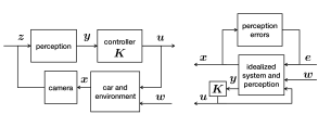
Figure 1: (Left) A diagram of the proposed perception-based control pipeline. (Right) The conceptual rearrangement of the closed-loop system permitted through our perception error characterization.

Suppose instead that there exists a perception map $p$ that imperfectly predicts partial state information; that is $p(z_{k})=Cx_{k}+e_{k}$ for $C\in\mathbb{R}^{\ell\times n}$ a known matrix, and error $e_{k}\in\mathbb{R}^{\ell}$. Using this map, we define a new measurement model in which the map $p$ plays the role of a noisy sensor:

$$y_{k}=p(z_{k})=Cx_{k}+e_{k}.$$ (4)

This allows us to reformulate problem (3) as a linear optimal control problem, where the measurements are defined by (4) and the control law $u_{k}=\bm{K}(y_{0:k})$ is a linear function of the outputs of past measurements $y_{0:k}$. As illustrated in Figure 1, guarantees of performance, safety, and robustness require designing a controller which suitably responds to system disturbance $\bm{w}$ and sensor noise $\bm{e}$. For linear optimal control problems, a variety of cost functions and noise models have well-understood solutions; we expand on this observation further in Section 2.1.

In light of this discussion, we approach our problem with the following data-driven procedure: First, we use supervised learning to fit a perception map and explicitly characterize its errors in terms of the data it was trained on. Second, we compute a robust controller that mitigates the effects of the measurement error $\bm{e}$. We will show that under suitable local smoothness assumptions on the generative model $q$ and perception map $p$ we can guarantee closed-loop robustness using a number of samples depending only on the state dimension.

2.1 Background on linear optimal control

We first recall some basic concepts from linear optimal control in the partially observed setting. In particular we consider the optimal control problem

$$\begin{array}[]{rl}\mbox{minimize}_{\bm{K}}&c(\bm{x},\bm{u})\\ \mbox{subject to}&x_{k+1}=Ax_{k}+Bu_{k}+Hw_{k}\\ &y_{k}=Cx_{k}+e_{k}\\ &u_{k}=\bm{K}(y_{0:k}),\end{array}$$ (5)

for $x_{k}$ the state, $u_{k}$ the control input, $w_{k}$ the process noise, $e_{k}$ the sensor noise, $\bm{K}$ a linear-time-invariant operator, and $c(\bm{x},\bm{u})$ a suitable cost function.

Control design depends on how the disturbance $\bm{w}$ and measurement error $\bm{e}$ are modeled, as well as performance objectives. By modeling the disturbance $\bm{w}$ and sensor noise $\bm{e}$ as being drawn from different signal spaces, and by choosing correspondingly suitable cost functions, we can incorporate practical performance, safety, and robustness considerations into the design process. For example, the well-studied LQG control problem minimizes the expected quadratic cost for user-specified positive definite matrices and normally distributed process and measurement noise. The resulting optimal estimation and control policy is to apply a static state feedback controller with the Kalman filter state estimate. The robust version of this problem considers instead the worst-case quadratic cost for $\ell_{2}$ or power-norm bounded noise. This is the $\mathcal{H}_{\infty}$ optimal control problem, which has a rich history [72].

As a final example, we recall the $\mathcal{L}_{1}$ optimal control problem, which seeks to minimize the $\ell_{\infty}\to\ell_{\infty}$ induced norm of a system. This formulation best accommodates real-time safety constraints and actuator saturation, which we motivate in the following example.

Example 2.2 (Waypoint Tracking).

Suppose that the control objective is to keep the system within a bounded distance of a sequence of waypoints at every timestep, and that the distance between sequential waypoints is bounded. Denoting the system state as $\bm{\xi}$ and the waypoint sequence as $\bm{r}$, the cost function is

$$c(\bm{\xi},\bm{u})=\sup_{\begin{subarray}{c}\lVert r_{k+1}-r_{k}\rVert_{\infty}\leq 1,\\ \|e_{k}\|_{\infty}\leq 1,k\geq 0\end{subarray}}\left\lVert\begin{matrix}Q^{1/2}(\xi_{k}-r_{k})\\ R^{1/2}u_{k}\end{matrix}\right\rVert_{\infty}\>.$$

If we specify costs by $Q=\mathrm{diag}{(1/q^{2}_{i})}$ and $R=\mathrm{diag}{(1/r^{2}_{i})}$, then as long as the optimal cost is less than 1, we can guarantee bounded tracking error $|\xi_{i,k}-r_{i,k}|\leq q_{i}$ and actuation $|u_{i,k}|\leq r_{i}$ for all possible realizations of the waypoint and sensor error processes. By defining an augmented state, i.e. $x_{k}:=[\xi_{k}-r_{k};r_{k}]$, and modeling waypoints as bounded disturbances, i.e. $w_{k}:=r_{k+1}-r_{k}$, we can reformulate this cost into a standard $\mathcal{L}_{1}$ optimal control problem.

In Appendix A, we provide further details on these optimal control problem formulations and solutions. Returning to the goals of perception-based control, it is clear that the perception errors $e_{k}$ will not follow a Gaussian distribution. Because this invalidates the optimality of the LQG control strategy, we focus on bounded norm assumptions, particularly for the case of $\mathcal{L}_{1}$ control.

3 Data-dependent perception error

In this section, we introduce a procedure to estimate regions for which a learned perception map can be used safely during operation. We first suppose access to initial training data $\mathcal{S}_{0}=\{(x_{i},z_{i})\}_{i=1}^{N_{0}}$, used to learn a perception map via any wide variety of traditional supervised methods. We then estimate safe regions around the training data, potentially using parameters learned from a second dataset. The result is a characterization of how quickly the learned perception map degrades as we move away from the initial training data.

We will describe the regions of the state space within which the sensing is reliable using a safe set which approximates sub-level sets of the error function $e(x)=p(q(x))-Cx$. We make this precise in the following Lemma, defining a safe set which is valid under an assumption that the error function is locally slope bounded around training data.

Lemma 3.1 (Closeness implies generalization).

Suppose that $p\circ q-C$ is locally $S$-slope bounded with a radius of $r$ around training datapoints. Define the safe set

$$\begin{split}\mathcal{X}_{\gamma}=\bigcup\limits_{(x_{d},z_{d})\in\mathcal{S}_{0}}\{x\in B_{r}(x_{d})~{}:~{}~{}~{}\|p(z_{d})-Cx_{d}\|+S\|x-x_{d}\|\leq\gamma\}\>.\end{split}$$ (6)

Then for any $(x,z)$ with $x\in\mathcal{X}_{\gamma}$, the perception error is bounded: $\lVert p(z)-Cx\rVert\leq\gamma$.

Proof:

The proof follows by a simple argument. For training data point $(x_{d},z_{d})$ such that $x_{d}\in B_{r}(x)$,

$$\lVert p(z)-Cx\rVert =\lVert p(q(x))-Cx-(p(q(x_{d}))-Cx_{d})+p(q(x_{d}))-Cx_{d}\rVert$$

$$\leq S\lVert x-x_{d}\rVert+\lVert p(q(x_{d}))-Cx_{d}\rVert\>.$$

The second line follows from the local slope bounded assumption. Then further choosing $x_{d}$ to correspond to minimizing over training data in the definition of $\mathcal{X}_{\gamma}$, we have

$$\lVert p(z)-Cx\rVert\leq S\lVert x-x_{d}\rVert+\lVert p(q(x_{d}))-Cx_{d}\rVert\leq\gamma\>.$$

$\square$

The validity of the safe set $\mathcal{X}_{\gamma}$ depends on bounding the slope of the error function locally around the training data. We remark that this notion of slope boundedness has connections to sector bounded nonlinearities, a classic setting for nonlinear system stability analysis [24].

Deriving the slope boundedness of the error function relies on the learned perception map as well as the underlying generative model, so we propose a second learning step to estimate a bound on $S$. We use an additional dataset composed of samples around each training data point: $\mathcal{S}_{N}=\cup_{x_{d}\in\mathcal{S}_{0}}\mathcal{S}_{x_{d}}$, where each $\mathcal{S}_{x_{d}}$ contains $N$ points densely sampled from $B_{r}(x_{d})$. For each $x_{d}$ in the training set, we then fix a radius $r$ and estimate $S$ with the maximum observed slope:

$$\widehat{S}_{x_{d}}=\max_{x_{i}\in\mathcal{S}_{x_{d}}}s(x_{i},x_{d})\>,\quad\textrm{where}~{}~{}s(x,x^{\prime})=\lVert e(x)-e(x^{\prime})\rVert/\lVert x-x^{\prime}\rVert.$$ (7)

By taking the maximum over training datapoints $x_{d}$, the slope bound $S$ can be estimated with $|\mathcal{S}_{0}|N$ samples.

Proposition 3.2.

Assume that the error function $p\circ q-C$ is locally $L$-Lipschitz for a radius $r$ around a training point $x_{d}$. Further assume that the true maximum slope $S_{x_{d}}:=\max_{x\in B_{r}(x_{d})}s(x,x_{d})$ is achieved by a point with distance from $x_{d}$ greater than $0<\tau\leq r$. Then for $\widehat{S}_{x_{d}}$ estimated with an $\varepsilon$-covering of $B_{r}(x_{d})$,

$$S_{x_{d}}\leq\widehat{S}_{x_{d}}(1+\varepsilon/\tau)+L\varepsilon/\tau\>.$$

Proof:

Let $e(x)=p(q(x))-Cx$. For $x_{*}\in\mbox{argmax}_{x\in B_{r}(x_{d})}s(x,x_{d})$, we have

$$S=\frac{\|e(x_{*})-e(x_{d})\|}{\|x_{*}-x_{d}\|}=\frac{\|e(x^{\prime})-e(x_{d})+e(x_{*})-e(x^{\prime})\|}{\|x_{*}-x_{d}\|}\leq\frac{s(x^{\prime},x_{d})\|x^{\prime}-x_{d}\|+L\|x_{*}-x^{\prime}\|}{\|x_{*}-x_{d}\|},$$

for $x^{\prime}$ in the $\varepsilon$ cover of $B_{r}(x_{d})$. Because $S$ can be achieved at least $\tau$ away from $x_{d}$, and $x_{*}$ is at most $\varepsilon$ away from x’, we can bound $S$ as

$$S\leq\frac{s(x^{\prime},x_{d})(\|x^{\prime}-x_{*}\|+\|x_{*}-x_{d}\|)-L\|x_{*}-x^{\prime}\|}{\|x_{*}-x_{d}\|}\leq\widehat{S}(1+\varepsilon/\tau)+L\varepsilon/\tau.$$

$\square$

This result shows that adding a margin to the observed slope bound $\widehat{S}$ provides an upper bound on $S$. This margin decreases with the number of samples $N$ and depends on an assumption about the local smoothness of the system. This estimation problem is similar to Lipschitz estimation, which has been widely studied with an eye towards optimization [60]. We note that Lipschitz smoothness is a stronger condition than our bounded slope condition, and requires several additional smoothness assumptions to estimate [69].

By combining Lemma 3.1 with Proposition 3.2, we estimate bounds on the perception errors within a neighborhood of the training data. In what follows, we use these local error bounds in robust control.

4 Analysis and synthesis of perception-based controllers

The local generalization result in Lemma 3.1 is useful only if the system remains close to states visited during training. In this section, we show that robust control can ensure that the system will remain close to training data so long as the perception map generalizes well. By then enforcing that the composition of the two bounds is a contraction, a natural notion of controller robustness emerges that guarantees favorable behavior and generalization. In what follows, we adopt an adversarial noise model and exploit the fact that we can design system behavior to bound how far the system deviates from states visited during training.

Recall that for a state-observation pair $(x,z)$, the perception error, defined as $e:=p(z)-Cx$, acts as additive noise to the measurement model $y=p(z)$. While standard linear control techniques can handle uniformly bounded errors, more care is necessary to further ensure that the system remains with a safe region of the state space, as determined by the training data. Through a suitable convex reformulation of the safe region, this goal can be addressed through receding horizon strategies (e.g. [66, 45]). While these methods are effective in practice, constructing terminal sets and ensuring a priori that feasible solutions exist is not an easy task. To make explicit connections between learning and control, we turn our analysis to a system level perspective on the closed-loop to characterize its sensitivity to noise.

4.1 System-level parametrization

The system level synthesis (SLS) framework, proposed by Wang et al. [67], provides a parametrization of our problem that makes explicit the effects of errors $\bm{e}$ on system behavior. Namely, for any controller that is a linear function of the history of system outputs, we can write the state and input as a convolution of the system noise and the closed-loop system responses $\{\Phi_{xw}(k),\Phi_{xe}(k),\Phi_{uw}(k),\Phi_{ue}(k)\}$,

$$\begin{bmatrix}x_{k}\\ u_{k}\end{bmatrix}=\sum_{t=1}^{k}\begin{bmatrix}\Phi_{xw}(t)&\Phi_{xe}(t)\\ \Phi_{uw}(t)&\Phi_{ue}(t)\end{bmatrix}\begin{bmatrix}Hw_{k-t}\\ e_{k-t}\end{bmatrix}\>.$$ (8)

As the equation (8) is linear in the system response elements $\Phi$, convex constraints on state and input translate to convex constraints on the system response elements. Wang et al. [67] show that for any elements $\{\Phi_{xw}(k),\Phi_{xe}(k),\Phi_{uw}(k),\Phi_{ue}(k)\}$ constrained to obey, for all $k\geq 1$,

$$\Phi_{xw}(1)=I,~{}~{}\begin{bmatrix}\Phi_{xw}(k+1)&\Phi_{xe}(k+1)\end{bmatrix} =A\begin{bmatrix}\Phi_{xw}(k)&\Phi_{xe}(k)\end{bmatrix}+B\begin{bmatrix}\Phi_{uw}(k)&\Phi_{ue}(k)\end{bmatrix},$$

$$\begin{bmatrix}\Phi_{xw}(k+1)\\ \Phi_{uw}(k+1)\end{bmatrix} =\begin{bmatrix}\Phi_{xw}(k)\\ \Phi_{uw}(k)\end{bmatrix}A+\begin{bmatrix}\Phi_{xe}(k+1)\\ \Phi_{ue}(k+1)\end{bmatrix}C\>,$$

there exists a feedback controller that achieves the desired system responses (8), and therefore any optimal control problem over linear systems can be cast as a corresponding optimization problem over system response elements.

To lessen the notational burden of working with these system response elements, we will work with their $z$ transforms. This is particularly useful for keeping track of semi-infinite sequences, especially since convolutions in time can now be represented as multiplications, i.e.

$$\begin{bmatrix}\bm{x}\\ \bm{u}\end{bmatrix}=\begin{bmatrix}\bm{\Phi}_{\bm{x}\bm{w}}&\bm{\Phi}_{\bm{x}\bm{e}}\\ \bm{\Phi}_{\bm{u}\bm{w}}&\bm{\Phi}_{\bm{u}\bm{e}}\end{bmatrix}\begin{bmatrix}H\bm{w}\\ \bm{e}\end{bmatrix}\>.$$

The corresponding control law $\bm{u}=\bm{K}\bm{y}$ is given by $\bm{K}=\bm{\Phi}_{\bm{u}\bm{e}}-\bm{\Phi}_{\bm{u}\bm{w}}\bm{\Phi}_{\bm{x}\bm{w}}^{-1}\bm{\Phi}_{\bm{x}\bm{e}}$. This controller can be implemented via a state-space realization [8] or as an interconnection of the system response elements [67]. The affine realizability constraints can be rewritten as

$$\begin{bmatrix}zI-A&-B\end{bmatrix}\bm{\Phi}=\begin{bmatrix}I&0\end{bmatrix},~{}~{}\bm{\Phi}\begin{bmatrix}zI-A\\ -C\end{bmatrix}=\begin{bmatrix}I\\ 0\end{bmatrix}\iff\bm{\Phi}\in\mathcal{A}\>,$$ (9)

where we denote the affine space defined by $(A,B,C)$ as $\mathcal{A}$.

In this SLS framework, many robust control costs can be written as system norms,

$$c(\bm{x},\bm{u})=\sup_{\begin{subarray}{c}\lVert\bm{w}\rVert\leq\varepsilon_{w}\\ \lVert\bm{e}\rVert\leq\varepsilon_{e}\end{subarray}}\left\|\begin{bmatrix}Q^{1/2}&\\ &R^{1/2}\end{bmatrix}\begin{bmatrix}\bm{\Phi}_{\bm{x}\bm{w}}&\bm{\Phi}_{\bm{x}\bm{e}}\\ \bm{\Phi}_{\bm{u}\bm{w}}&\bm{\Phi}_{\bm{u}\bm{e}}\end{bmatrix}\begin{bmatrix}H\bm{w}\\ \bm{e}\end{bmatrix}\right\|=\left\|\begin{bmatrix}Q^{1/2}&\\ &R^{1/2}\end{bmatrix}\begin{bmatrix}\bm{\Phi}_{\bm{x}\bm{w}}&\bm{\Phi}_{\bm{x}\bm{e}}\\ \bm{\Phi}_{\bm{u}\bm{w}}&\bm{\Phi}_{\bm{u}\bm{e}}\end{bmatrix}\begin{bmatrix}\varepsilon_{w}H\\ \varepsilon_{e}I\end{bmatrix}\right\|\>.$$

For LQG control, the objective is equivalent to a system $\mathcal{H}_{2}$ norm [72].

A comment on finite-dimensional realizations

Although the constraints and objective function in this framework are infinite dimensional, two finite-dimensional approximations have been successfully applied. The first consists of selecting an approximation horizon $T$, and enforcing that $\bm{\Phi}(T)=0$ for some appropriately large $T$, which is always possible for systems that are controllable and observable. When this is not possible, one can instead enforce bounds on the norm of $\bm{\Phi}(T)$ and use robustness arguments to show that the sub-optimality gap incurred by this finite dimensional approximation decays exponentially in the approximation horizon $T$ [9, 14, 22, 44]. Finally, in the interest of clarity, we always present the infinite horizon version of the optimization problems, with the understanding that finite horizon approximations are necessary in practice.

4.2 Robust control for generalization

In what follows, we specialize controller design concerns to our perception-based setting, and develop further conditions on the closed-loop response $\bm{\Phi}$ to incorporate into the synthesis problem. Because system level parametrization makes explicit the effects of perception errors $\bm{e}$ on system behavior, we can transparently keep track of closed-loop behavior, as made precise in the following Lemma.

Lemma 4.1 (Generalization implies closeness).

For a perception map $p$ with errors $\bm{e}=p(\bm{z})-C\bm{x}$, let the system responses $\left\{\bm{\Phi}_{\bm{x}\bm{w}},\bm{\Phi}_{\bm{x}\bm{e}},\bm{\Phi}_{\bm{u}\bm{w}},\bm{\Phi}_{\bm{u}\bm{e}}\right\}$ lie in the affine space defined by dynamics $(A,B,C)$, and let $\bm{K}$ be the associated controller. Then the state trajectory $\bm{x}$ achieved by the control law $\bm{u}=\bm{K}p(\bm{z})$ and driven by noise process $\bm{w}$, satisfies, for any target trajectory $\bm{x}_{d}$,

$$\lVert\bm{x}-\bm{x}_{d}\rVert\leq\lVert\widehat{\bm{x}}-\bm{x}_{d}\rVert+\lVert\bm{\Phi}_{\bm{x}\bm{e}}\rVert\lVert\bm{e}\rVert.$$ (10)

where we define the nominal closeness $\lVert\widehat{\bm{x}}-\bm{x}_{d}\rVert=\lVert\bm{\Phi}_{\bm{x}\bm{w}}H\bm{w}-\bm{x}_{d}\rVert$ to be the deviation from the target trajectory in the absence of measurement errors.

Proof:

Notice that over the course of a trajectory, we have system outputs $\bm{y}=p(\bm{z})=C\bm{x}+\bm{e}$. Then recalling that the system responses are defined such that $\bm{x}=\bm{\Phi}_{\bm{x}\bm{w}}H\bm{w}+\bm{\Phi}_{\bm{x}\bm{e}}\bm{e}$, we have that

$$\lVert\bm{x}-\bm{x}_{d}\rVert =\lVert\bm{\Phi}_{\bm{x}\bm{w}}H\bm{w}+\bm{\Phi}_{\bm{x}\bm{e}}\bm{e}-\bm{x}_{d}\rVert\leq\lVert\bm{\Phi}_{\bm{x}\bm{w}}H\bm{w}-\bm{x}_{d}\rVert+\lVert\bm{\Phi}_{\bm{x}\bm{e}}\rVert\lVert\bm{e}\rVert\>.$$

$\square$

The terms in bound (10) capture different generalization properties. The first is small if we plan to visit states during operation that are similar to those seen during training. The second term is a measure of the robustness of our system to the error $\bm{e}$.

We are now in a position to state the main result of the paper, which shows that under an additional robustness condition, Lemmas 3.1 and 4.1 combine to define a control invariant set around the training data within which we can bound the perception errors and consequently the performance.

Theorem 4.2.

Let the assumptions of Lemmas 3.1 and 4.1 hold and suppose that the training error is bounded, i.e. $\|p(z_{d})-Cx_{d}\|\leq R_{0}$ for all $(x_{d},z_{d})\in\mathcal{S}_{0}$. Then as long as

$$\lVert\bm{\Phi}_{\bm{x}\bm{e}}\rVert\leq\frac{1-\frac{1}{r}\lVert\widehat{\bm{x}}-\bm{x}_{d}\rVert}{S+\frac{R_{0}}{r}}\>,$$ (11)

the perception errors remain bounded

$$\lVert p(\bm{z})-C\bm{x}\rVert\leq\frac{\lVert\widehat{\bm{x}}-\bm{x}_{d}\rVert+R_{0}}{1-S\lVert\bm{\Phi}_{\bm{x}\bm{e}}\rVert}:=\gamma,$$ (12)

and the closed-loop trajectory lies within $\mathcal{X}_{\gamma}$.

Proof:

Recall that as in the proof of Lemma 3.1, as long as $x_{k}\in B_{r}(x_{d,k})$ for all $k$ and some arbitrary $x_{d,k}\in\mathcal{S}_{0}$,

$$\|e_{k}\|\leq S\|x_{k}-x_{d,k}\|+\|e_{d_{k}}\|\implies\|\bm{e}\|=\max_{k}\|e_{k}\|\leq S\|\bm{x}-\bm{x}_{d}\|+\|\bm{e}_{d}\|\>.$$ (13)

By assumption, $\|\bm{e}_{d}\|\leq R_{0}$. Substituting this expression into the result of Lemma 4.1, we see that as long as $\|x_{k}-x_{d,k}\|\leq r$ for all $k$,

$$\lVert\bm{x}-\bm{x}_{d}\rVert\leq\lVert\widehat{\bm{x}}-\bm{x}_{d}\rVert+\lVert\bm{\Phi}_{\bm{x}\bm{e}}\rVert(S\|\bm{x}-\bm{x}_{d}\|+\|\bm{e}_{d}\|)\iff\lVert\bm{x}-\bm{x}_{d}\rVert\leq\frac{\lVert\widehat{\bm{x}}-\bm{x}_{d}\rVert+\varepsilon_{\eta}\lVert\bm{\Phi}_{\bm{x}\bm{e}}\rVert}{1-S\lVert\bm{\Phi}_{\bm{x}\bm{e}}\rVert}\>,$$

Next, to ensure that the the radius is bounded, first note that by norm definition, $\max_{k}\|x_{k}-x_{d,k}\|_{\infty}\leq r$ if and only if $\|\bm{x}-\bm{x}_{d}\|\leq r$. A sufficient condition for this is given by

$$\frac{\lVert\widehat{\bm{x}}-\bm{x}_{d}\rVert+R_{0}\lVert\bm{\Phi}_{\bm{x}\bm{e}}\rVert}{1-S\lVert\bm{\Phi}_{\bm{x}\bm{e}}\rVert}\leq r\iff\lVert\bm{\Phi}_{\bm{x}\bm{e}}\rVert\leq\frac{1-\frac{1}{r}\lVert\widehat{\bm{x}}-\bm{x}_{d}\rVert}{S+\frac{R_{0}}{r}}\>,$$

and thus we arrive at the robustness condition. Since the bound on $\lVert\bm{x}-\bm{x}_{d}\rVert$ is valid, we now use it to bound $\|\bm{e}\|$, starting with (13) and rearranging,

$$\|\bm{e}\|\leq\frac{\lVert\widehat{\bm{x}}-\bm{x}_{d}\rVert+R_{0}}{1-S\lVert\bm{\Phi}_{\bm{x}\bm{e}}\rVert}\>.$$

$\square$

Theorem 4.2 shows that the bound (11) should be used during controller synthesis to ensure generalization. Feasibility of the synthesis problem depends on the controllability and observability of the system $(A,B,C)$, which impose limits on how small $\lVert\bm{\Phi}_{\bm{x}\bm{e}}\rVert$ can be made to be, and on the planned deviation from training data as captured by the quantity $\lVert\widehat{\bm{x}}-\bm{x}_{d}\rVert$.

4.3 Robust synthesis for waypoint tracking

We now specialize to the task of waypoint tracking to simplify the term $\lVert\widehat{\bm{x}}-\bm{x}_{d}\rVert$ and propose a robust control synthesis problem. Recall that waypoint tracking can be encoded by defining the state $x_{k}:=[\xi_{k}-r_{k};r_{k}]$ as the concatenation of tracking error and waypoint and the disturbance as the change in reference, $w_{k}:=r_{k+1}-r_{k}$.

Proposition 4.3.

For a reference tracking problem with $\|r_{k+1}-r_{k}\|\leq\Delta_{\mathrm{ref}}$ and a reference trajectory within a ball of radius $r_{\mathrm{ref}}$ from the training data,

$$\lVert\widehat{\bm{x}}-\bm{x}_{d}\rVert\leq\Delta_{\mathrm{ref}}\|\begin{bmatrix}I&0\end{bmatrix}\bm{\Phi}_{\bm{x}\bm{w}}H\|+r_{\mathrm{ref}}\>.$$

Proof:

For the training data, we can assume zero tracking errors, so that $\bm{\xi}_{d}=\bm{r}_{d}$. Then $x_{d,k}=[0;\xi_{d,k}]$. Thus, we can rewrite $\lVert\widehat{\bm{x}}-\bm{x}_{d}\rVert\leq\|\bm{\xi}-\bm{r}\|+\|\bm{r}-\bm{\xi}_{d}\|=\|\begin{bmatrix}I&0\end{bmatrix}\bm{\Phi}_{\bm{x}\bm{w}}\bm{w}\|+\|\bm{r}-\bm{\xi}_{d}\|$. $\square$

Using this setting, we add the robustness condition in (11) to a control synthesis problem as

$$\begin{array}[]{rl}\mbox{minimize}_{\bm{\Phi}}&c(\bm{\Phi})\\ \mbox{subject to}&\bm{\Phi}\in\mathcal{A},~{}~{}(S+\frac{R_{0}}{r})\lVert\bm{\Phi}_{\bm{x}\bm{e}}\rVert+\frac{\Delta_{\mathrm{ref}}}{r}\|\begin{bmatrix}I&0\end{bmatrix}\bm{\Phi}_{\bm{x}\bm{w}}H\|+\frac{r_{\mathrm{ref}}}{r}\leq 1\>.\end{array}$$

Notice the trade-off between the size of different parts of the system response. Because the responses must lie in an affine space, they cannot both become arbitrarily small. Therefore, the synthesis problem must trade off between sensitivity to measurement errors and tracking fidelity. These trade-offs are mediated by the quality of the perception map, through its slope-boundedness and training error, and the ambition of the control task, through its deviation from training data and distances between waypoints.

While the robustness constraint in (11) is enough to guarantee a finite cost, it does not guarantee a small cost. To achieve this, we incorporate the error bound to arrive at the following robust synthesis procedure:

$$\begin{array}[]{rl}\mbox{minimize}_{\bm{\Phi},\gamma}&\left\|\begin{bmatrix}Q^{1/2}&\\ &R^{1/2}\end{bmatrix}\begin{bmatrix}\bm{\Phi}_{\bm{x}\bm{w}}&\bm{\Phi}_{\bm{x}\bm{e}}\\ \bm{\Phi}_{\bm{u}\bm{w}}&\bm{\Phi}_{\bm{u}\bm{e}}\end{bmatrix}\begin{bmatrix}\Delta_{\mathrm{ref}}H\\ \gamma I\end{bmatrix}\right\|\\ \mbox{subject to}&\bm{\Phi}\in\mathcal{A},~{}~{}(S+\frac{R_{0}}{r})\lVert\bm{\Phi}_{\bm{x}\bm{e}}\rVert+\frac{\Delta_{\mathrm{ref}}}{r}\|\begin{bmatrix}I&0\end{bmatrix}\bm{\Phi}_{\bm{x}\bm{w}}H\|+\frac{r_{\mathrm{ref}}}{r}\leq 1\\ &\Delta_{\mathrm{ref}}\|\begin{bmatrix}I&0\end{bmatrix}\bm{\Phi}_{\bm{x}\bm{w}}H\|+r_{\mathrm{ref}}+R_{0}\leq\gamma(1-S\lVert\bm{\Phi}_{\bm{x}\bm{e}}\rVert)\>.\end{array}$$

This is a convex program for fixed $\gamma$, so the full problem can then be approximately solved via one-dimensional search.

4.4 Necessity of robustness

Robust control is notoriously conservative, and our main result reslies heavily on small gain-like arguments. Can the conservatism inherent in this approach be generally reduced? In this section, we answer in the negative by describing a class of examples for which the robustness condition in Theorem 4.2 is necessary. For simplicity, we specialize to the goal of regulating a system to the origin, and assume that $(0,z_{0})$ is in the training set, with $p(z_{0})=0$.

We consider the following optimal control problem

$$\begin{array}[]{rl}\mbox{minimize}_{\bm{\Phi}}&c(\bm{\Phi})~{}~{}\mbox{subject to}~{}~{}\bm{\Phi}\in\mathcal{A},~{}~{}\|\bm{\Phi}_{\bm{x}\bm{e}}\|\leq\alpha\>.\end{array}$$

and define $\bar{\bm{\Phi}}$ as a minimizing argument for the problem without the inequality constraint. For simplicity, we consider only systems in which the closed-loop is strictly proper and has a state-space realization.

Proposition 4.4.

Suppose that

$$\|\bar{\bm{\Phi}}_{\bm{xn}}\|_{\mathcal{L}_{1}}=\|\bar{\bm{\Phi}}_{\bm{xn}}(1)\|_{\infty\to\infty}\>.$$

Then there exists a differentiable error function with slope bound $S$ such that $x=0$ is an asymptotically stable equilibrium if and only if $\alpha<\frac{1}{S}$.

Proof:

Sufficiency follows from our main analysis, or alternatively from a simple application of the small gain theorem. The necessity follows by construction, with a combination of classic nonlinear instability arguments and by considering real stability radii.

Recall that $y_{k}=Cx_{k}+(p(q(x_{k}))-Cx_{k})$. Define $\zeta_{k}$ to represent the internal state of the controller. Then we can write the system’s closed-loop behavior as (ignoring for now the effect of process noise, which does not affect the stability analysis)

$$\begin{bmatrix}x_{k+1}\\ \zeta_{k+1}\end{bmatrix}=A_{\mathrm{CL}}\begin{bmatrix}x_{k}\\ \zeta_{k}\end{bmatrix}+B_{\mathrm{CL}}e(x_{k})\>.$$

Suppose that the error function $e(x)$ is differentiable at $x=0$ with derivative $J$. Then the stability of the origin depends on the linearized closed loop system $A_{\mathrm{CL}}(J):=A_{\mathrm{CL}}+B_{\mathrm{CL}}JC_{\mathrm{CL}}$ where $C_{\mathrm{CL}}=[I~{}0]$ picks out the relevant component of the closed-loop state. If any eigenvalues of $A_{\mathrm{CL}}(J)$ lie outside of the unit disk, then $x=0$ is not an asymptotically stable equilibrium.

Switching gears, recall that ${\bm{\Phi}}_{\bm{x}\bm{e}}(z)=C_{\mathrm{CL}}(zI-A_{\mathrm{CL}})^{-1}B_{\mathrm{CL}}$. We define $S=1/\|\bar{\bm{\Phi}}_{\bm{xe}}\|$ and notice that if $\alpha\geq\frac{1}{S}$, then $\bar{\bm{\Phi}}$ is also the solution to the constrained problem. By assumption, $\|\bar{\bm{\Phi}}_{\bm{xn}}\|_{\mathcal{L}_{1}}=\|\bar{\bm{\Phi}}_{\bm{xn}}(1)\|_{\infty\to\infty}$. Thus, there exist real $w,v$ such that $v^{\top}\bar{\bm{\Phi}}_{\bm{xn}}(1)w=\|\bar{\bm{\Phi}}_{\bm{xn}}\|$. If we set $J=Swv^{\top}$, then $A_{\mathrm{CL}}(J)$ has an eigenvalue on the unit disk and $x=0$ is not an asymptotically stable equilibrium. To see why this is true, recall the classic result for stability radii (e.g. Corollary 4.5 in Hinrichsen and Pritchard [33]) and notice

$$\bar{\bm{\Phi}}_{\bm{xn}}(1)=\sum_{k\geq 0}\Phi_{xn}(k)=\sum_{k\geq 0}C_{\mathrm{CL}}A_{\mathrm{CL}}^{k}B_{\mathrm{CL}}=C_{\mathrm{CL}}(I-A_{\mathrm{CL}})^{-1}B_{\mathrm{CL}}\>.$$

Thus, for any error function with derivative $J=Swv^{\top}$ at zero, the robustness condition is necessary as well as sufficient. One such error function is simply $e(x)=Jx$, though many more complex forms exist. $\square$

We now present a simple example in which this condition is satisfied, and construct the corresponding error function which results in an unstable system.

Example

Consider the double integrator

$$x_{k+1}=\begin{bmatrix}1&dt\\ 0&1\end{bmatrix}x_{k}+\begin{bmatrix}0\\ 1\end{bmatrix}u_{k},\quad y_{k}=p(z_{k})=x_{k}+e(x_{k})\>,$$ (14)

and the control law resulting from the $\mathcal{H}_{2}$ optimal control problem with identity weighting matrices along with the robustness constraint $\|\bm{\Phi}_{\bm{x}\bm{e}}\|\leq\alpha$. Notice that the solution to the unconstrained problem would be the familiar LQG combination of Kalman filtering and static feedback on the estimated state. We denote the optimal unconstrained system response by $\bar{\bm{\Phi}}$.

Consider an error function with slope bounded by $S=1/{\|\bar{\bm{\Phi}}_{\bm{x}\bm{e}}\|}$ and derivative at $x=0$ equal to

$$J=\begin{bmatrix}-1/{\|\bar{\bm{\Phi}}_{\bm{x}\bm{e}}\|}&0\\ -1/{\|\bar{\bm{\Phi}}_{\bm{x}\bm{e}}\|}&0\end{bmatrix}\>,$$

Calculations confirm that the $\mathcal{L}_{1}$ norm satisfies the relevant property and that the origin is not a stable fixed point if the synthesis constraint $\alpha\geq\frac{1}{S}$.

5 Experiments

We demonstrate our theoretical results with examples of control from pixels, using both simple synthetic images and complex graphics simulation. The synthetic example uses generated $64\times 64$ pixel images of a moving blurry white circle on a black background; the complex example uses $800\times 600$ pixel dashboard camera images of a vehicle in the CARLA simulator platform [25].

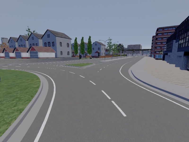
Figure 2: In (a), visual inputs $\{z_{t}\}$ for the synthetic (left) and CARLA (right) examples. In (b), (left) the $\ell_{\infty}$ bounded ball the synthetic circle must remain inside in the face of bounded adversarial noise, (center) the nominal trajectory the synthetic circle is driven to follow, and (right) and the nominal trajectory the simulated vehicle is driven to follow.

Figure 2(a) shows representative images seen by the controllers.

For both visual settings, we demonstrate our results in controlling a 2D double integrator to track a periodic reference. The 2D double integrator state is given by $x_{k}^{\top}=[(x_{k}^{(1)})^{\top}\,(x_{k}^{(2)})^{\top}]$, and each component evolves independently according to the dynamics in (14) with $dt=0.1$. For all examples, the sensing matrix $C$ extracts the position of the system, i.e., $Cx_{k}=[x^{(1)}_{1,k},x^{(2)}_{1,k}]$. Training and validation trajectories are generated by driving the system with an optimal state feedback controller (i.e. where measurement $\bm{y}=\bm{x}$) to track a desired reference trajectory $\bm{w}=\bm{r}+\bm{v}$, where $\bm{r}$ is a nominal reference, and $\bm{v}$ is a random norm bounded random perturbation satisfying $\lVert v_{k}\rVert_{\infty}\leq 0.1$.

We consider three different perception maps: a linear map for the synthetic example and both visual odometry and a convolutional neural net for the CARLA example. For the CNN, we collect a dense set of training examples around the reference to train the model. We use the approach proposed by Coates and Ng [18] to learn a convolutional representation of each image: each resized and scaled image is passed through a single convolutional, ReLU activation, and max pooling layer. We then fit a linear map of these learned image features to position and heading of the camera pose. We require approximately $30000$ training points. During operation, pixel-data $z$ is passed through the CNN to obtain position estimates $y$, which are then used by the robust controller. We note that other more sophisticated architectures for feature extraction would also be reasonable to use in our control framework; we find that this one is conceptually simple and sufficient for tracking around our fixed reference.

To perform visual odometry, we first collect images from known poses around the desired reference trajectory. We then use ORB SLAM [46] to build a global map of visual features and a database of reference images with known poses. This is the “training” phase. We use one trajectory of $200$ points; the reference database is approximately this size. During operation, an image $z$ is matched with an image $z_{d}$ in the database. The reprojection error between the matched features in $z_{d}$ with known pose $x_{d}$ and their corresponding features in $z$ is then minimized to generate pose estimate $y$. For more details on standard visual odometry methods, see [59]. We highlight that modern visual SLAM algorithms incorporate sophisticated filtering and optimization techniques for localization in previously unseen environments with complex dynamics; we use a simplified algorithm under this training and testing paradigm in order to better isolate the data dependence.

We then estimate safe regions for all three maps, as described in Section 3. In the top panels of Figure 3 we show the error profiles as a function of distance to the nearest training point for the linear (left), SLAM (middle), and CNN (right) maps. We see that these data-dependent localization schemes exhibit the local slope bounded property posited in the previous section.

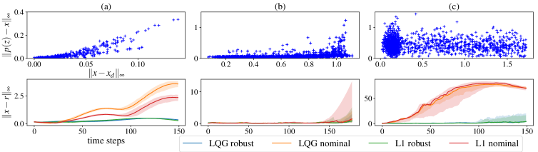
Figure 3: (top) Test perception error $\|p(z)-Cx\|_{\infty}$ vs. distance to the nearest training point $\|x-x_{d}\|_{\infty}$; and (bottom) median $\ell_{\infty}$ tracking error for 200 rollouts using the (a) linear map on synthetic images, (b) SLAM and (c) CNN on CARLA dashboard images. Error bars show upper and lower quartiles.

We compare robust synthesis to the behavior of nominal controllers that do not take into account the nonlinearity in the measurement model. In particular, we compare the performance of naively synthesized LQG and $\mathcal{L}_{1}$ optimal controllers with controllers designed with the robustness condition (11). LQG is a standard control scheme that explicitly separates state estimation (Kalman Filtering) from control (LQR control), and is emblematic of much of standard control practice. $\mathcal{L}_{1}$ optimal control minimizes worst case state deviation and control effort by modeling process and sensor errors as $\ell_{\infty}$ bounded adversarial processes. For further discussion and details, refer to Section 2.1 and Appendix B. The bottom panels of Figure 3 show that the robustly synthesized controllers remain within a bounded neighborhood around the training data. On the other hand, the nominal controllers drive the system away from the training data, leading to a failure of the perception and control loop. We note that although visual odometry may not satisfy smoothness assumptions when the feature detection and matching fails, we nevertheless observe safe system behavior, suggesting that using our robust controller, no such failures occur.

6 Conclusion

Though standard practice is to treat the output of a perception module as an ordinary signal, we have demonstrated both in theory and experimentally that accounting for the inherent uncertainty of perception based sensors can dramatically improve the performance of the resulting control loop. Moreover, we have shown how to quantify and account for such uncertainties with tractable data-driven safety guarantees. We hope to extend this study to the control of more complex systems, and to apply this framework to standard model-predictive control pipelines which form the basis of much of contemporary control practice.

We further hope to highlight the challenges involved in adapting learning-theoretic notions of generalization to the setting of controller synthesis. First note that if we collect data using one controller, and then use this data to build a new controller, there will be a distribution shift in the observations seen between the two controllers. Any statistical generalization bounds on performance must necessarily account for this shift. Second, from a more practical standpoint, most generalization bounds require knowing instance specific quantities governing properties of the class of functions we use to fit a predictor. Hence, they will include constants that are not measurable in practice. This issue can perhaps be mitigated using some sort of bootstrap technique for post-hoc validation. However, we note that the sort of bounds we aim to bootstrap are worst case, not average case. Indeed, the bootstrap typically does not even provide a consistent estimate of the maximum of independent random variables, see for instance [13], and Ch 9.3 in [17]. Other measures such as conditional value at risk require billions of samples to guarantee five 9s of reliability  [54]. We highlight these issues only to point out that adapting statistical generalization to robust control is an active area with many open challenges to be considered in future work.

Acknowledgments

This work is generously supported in part by ONR awards N00014-17-1-2191, N00014-17-1-2401, and N00014-18-1-2833, the DARPA Assured Autonomy (FA8750-18-C-0101) and Lagrange (W911NF-16-1-0552) programs, a Siemens Futuremakers Fellowship, and an Amazon AWS AI Research Award. SD and VY are supported by an NSF Graduate Research Fellowship under Grant No. DGE 1752814.

Appendix A Linear optimal control

Name	Disturbance class	Cost function	Use cases
LQR/$\mathcal{H}_{2}$	$\mathbb{E}\nu=0,$ $\mathbb{E}\nu^{4}<\infty$, $\nu_{k}$ i.i.d.	$\displaystyle\mathbb{E}_{\nu}\left[\lim_{T\to\infty}\sum_{k=0}^{T}\frac{1}{T}x_{k}^{\top}Qx_{k}+u_{k}^{\top}Ru_{k}\right]$	Sensor noise, aggregate behavior, natural processes
$\mathcal{H}_{\infty}$	$\lVert\nu\rVert_{pow}\leq 1$	$\displaystyle\sup_{\lVert\nu\rVert_{pow}\leq 1}\lim_{T\to\infty}\frac{1}{T}\sum_{k=0}^{T}x_{k}^{\top}Qx_{k}+u_{k}^{\top}Ru_{k}$	Modeling error, energy/power constraints
$\mathcal{L}_{1}$	$\lVert\nu\rVert_{\infty}\leq 1$	$\displaystyle\sup_{\lVert\nu\rVert_{\infty}\leq 1,k\geq 0}\left\lVert\begin{matrix}Q^{1/2}x_{k}\\ R^{1/2}u_{k}\end{matrix}\right\rVert_{\infty}$	Real-time safety constraints, actuator saturation/limits

Table 1: Different noise model classes induce different cost functions, and can be used to model different phenomenon, or combinations thereof [72, 21].

Table 1 shows several common cost functions that arise from different system desiderata and different classes of disturbances and measurement errors $\nu:=(w,e)$. We recall the power norm, defined as

$$\lVert\bm{x}\rVert_{pow}:=\sqrt{\lim_{T\to\infty}\frac{1}{T}\sum_{k=0}^{T}\lVert x_{k}\rVert_{2}^{2}}\>.$$

We now recall some examples from linear optimal control in the partially observed setting.

Example A.1 (Linear Quadratic Regulator).

Suppose that the cost function is given by

$$c(\bm{x},\bm{u})=\mathbb{E}_{\nu}\left[\lim_{T\to\infty}\frac{1}{T}\sum_{k=0}^{T}x_{k}^{\top}Qx_{k}+u_{k}^{\top}Ru_{k}\right],$$

for some user-specified positive definite matrices $Q$ and $R$, $w_{k}\stackrel{{\scriptstyle\mathclap{\text{\scriptsize{ \tiny i.i.d.}}}}}{{\sim}}\mathcal{N}(0,I)$, $H=I$, and that the controller is given full information about the system, i.e., that $C=I$ and $e_{k}=0$ such that the measurement model collapses to $y_{k}=x_{k}$. Then the optimal control problem reduces to the familiar Linear Quadratic Regulator (LQR) problem

$$\begin{array}[]{rl}\displaystyle\mbox{minimize}_{\{\pi\}}&\mathbb{E}_{w}\left[\displaystyle\lim_{T\to\infty}\frac{1}{T}\sum_{k=0}^{T}x_{k}^{\top}Qx_{k}+u_{k}^{\top}Ru_{k}\right]\\ \mathrm{subjectto}&x_{k+1}=Ax_{k}+Bu_{k}+w_{k}\\ &u_{k}=\pi(x_{0:k}),\end{array}$$ (15)

For stabilizable $(A,B)$, and detectable $(A,Q)$, this problem has a closed-form stabilizing controller based on the solution of the discrete algebraic Riccati equation (DARE) [72]. This optimal control policy is linear, and given by

$$u^{\mathrm{LQR}}_{k}=-(B^{\top}PB+R)^{-1}B^{\top}PAx_{k}=:K_{\mathrm{LQR}}x_{k},$$ (16)

where $P$ is the positive-definite solution to the DARE defined by $(A,B,Q,R)$.

Example A.2 (Linear Quadratic Gaussian Control).

Suppose that we have the same setup as the previous example, but that now the measurement is instead given by (4) for some $C$ such that the pair $(A,C)$ is detectable, and that $e_{k}\stackrel{{\scriptstyle\mathclap{\text{\scriptsize{ \tiny i.i.d.}}}}}{{\sim}}\mathcal{N}(0,I)$. Then the optimal control problem reduces to the Linear Quadratic Gaussian (LQG) control problem, the solution to which is:

$$u^{\mathrm{LQG}}_{k}=K_{\mathrm{LQR}}\hat{x}_{k},$$ (17)

where $\hat{x}_{k}$ is the Kalman filter estimate of the state at time $k$. The steady state update rule for the state estimate is given by

$$\hat{x}_{k+1}=A\hat{x}_{k}+Bu_{k}+L_{\mathrm{LQG}}(y_{k+1}-C(A\widehat{x}_{k}+Bu_{k}))$$

for filter gain $L_{\mathrm{LQG}}=-PC^{\top}(CPC^{\top}+I)^{-1}$ where $P$ is the solution to the DARE defined by $(A^{\top},C^{\top},I,I)$. This optimal output feedback controller satisfies the separation principle, meaning that the optimal controller $K_{\mathrm{LQR}}$ is computed independently of the optimal estimator gain $L_{\mathrm{LQG}}$.

These first two examples are widely known due to the elegance of their closed-form solutions and the simplicity of implementing the optimal controllers. However, this optimality rests on stringent assumptions about the distribution of the disturbance and the measurement noise. We now turn to an example, first introduced in Example 2.2, for which disturbances are adversarial and the separation principle fails.

Consider a waypoint tracking problem where it is known that both the distances between waypoints and sensor errors are instantaneously $\ell_{\infty}$ bounded, and we want to ensure that the system remains within a bounded distance of the waypoints. In this setup, the $\mathcal{L}_{1}$ optimal control problem is most natural, and our cost function is then

$$c(\bm{x},\bm{u})=\sup_{\begin{subarray}{c}\lVert r_{k+1}-r_{k}\rVert_{\infty}\leq 1,\\ \|e_{k}\|_{\infty}\leq 1,k\geq 0\end{subarray}}\left\lVert\begin{matrix}Q^{1/2}(x_{k}-r_{k})\\ R^{1/2}u_{k}\end{matrix}\right\rVert_{\infty},$$

for some user-specified positive definite matrices $Q=\mathrm{diag}{\frac{1}{q^{2}_{i}}}$ and $R=\mathrm{diag}{\frac{1}{r^{2}_{i}}}$. Then if the optimal cost is less than 1, we can guarantee that $|x_{i,k}-r_{i,k}|\leq q_{i}$ and $|u_{i,k}|\leq r_{i}$ for all possible realizations of the waypoint and sensor error processes. Considering the one-step lookahead case, we can define the augmented state $\xi_{k}=[x_{k}-r_{k};r_{k}]$ and pose the problem with bounded disturbances $w_{k}=r_{k+1}-r_{k}$. We can then formulate the following $\mathcal{L}_{1}$ optimal control problem,

$$\begin{array}[]{rl}\displaystyle\mbox{minimize}_{\{\pi\}}&\sup_{\lVert\nu\rVert_{\infty}\leq 1,k\geq 0}\left\lVert\begin{matrix}\bar{Q}^{1/2}\xi_{k}\\ R^{1/2}u_{k}\end{matrix}\right\rVert_{\infty}\\ \text{subject to}&\xi_{k+1}=\bar{A}\xi_{k}+\bar{B}u_{k}+\bar{H}w_{k}\>,~{}~{}y_{k}=\bar{C}\xi_{k}+\eta_{k}\\ &u_{k}=\pi(y_{0:k}),\end{array}$$ (18)

where

$$~{}~{}\bar{A}=\begin{bmatrix}A&0\\ 0&I\end{bmatrix},~{}~{}\bar{B}=\begin{bmatrix}B\\ 0\end{bmatrix},~{}~{}\bar{C}=\begin{bmatrix}C&0\end{bmatrix},~{}~{}\bar{H}=\begin{bmatrix}0\\ I\end{bmatrix}$$

This optimal control problem is an instance of $\mathcal{L}_{1}$ robust control [21]. The optimal controller does not obey the separation principle, and as such, there is no clear notion of an estimated state.

Appendix B Experimental details

The robust SLS procedure we propose and analyze requires solving a finite dimensional approximation to an infinite dimensional optimization problem, as $\left\{\bm{\Phi}_{\bm{x}\bm{w}},\bm{\Phi}_{\bm{x}\bm{e}},\bm{\Phi}_{\bm{u}\bm{w}},\bm{\Phi}_{\bm{u}\bm{e}}\right\}$ and the corresponding constraints (9) and objective function are infinite dimensional objects. As an approximation, we restrict the system responses $\left\{\bm{\Phi}_{\bm{x}\bm{w}},\bm{\Phi}_{\bm{x}\bm{e}},\bm{\Phi}_{\bm{u}\bm{w}},\bm{\Phi}_{\bm{u}\bm{e}}\right\}$ to be finite impulse response (FIR) transfer matrices of length $T=200$, i.e., we enforce that $\bm{\Phi}(T)=0$. We then solve the resulting optimization problem with MOSEK under an academic license [10]. More explicitly, we define $\mbox{vec}(\bm{F}):=\begin{bmatrix}F_{0}^{\top}&\dots&F_{T-1}^{\top}\end{bmatrix}^{\top}$ and $\overline{\mbox{vec}}(\bm{F}):=\begin{bmatrix}F_{0}&\dots&F_{T-1}\end{bmatrix}$, where $F_{t}$ are the FIR coefficients of the system responses. We further define

$$\bm{Z}:=\begin{bmatrix}Q^{1/2}&\\ &R^{1/2}\end{bmatrix}\begin{bmatrix}\bm{\Phi}_{\bm{x}\bm{w}}&\bm{\Phi}_{\bm{x}\bm{e}}\\ \bm{\Phi}_{\bm{u}\bm{w}}&\bm{\Phi}_{\bm{u}\bm{e}}\end{bmatrix}\begin{bmatrix}H\\ \gamma I\end{bmatrix}.$$ (19)

The SLS constraints (9) and FIR condition are then enforced as

$$\begin{split}&\begin{bmatrix}\overline{\mbox{vec}}(\bm{\Phi}_{\bm{x}\bm{w}})&0\end{bmatrix}-\begin{bmatrix}0&A\overline{\mbox{vec}}(\bm{\Phi}_{\bm{x}\bm{w}})\end{bmatrix}=\begin{bmatrix}0&B\overline{\mbox{vec}}(\bm{\Phi}_{\bm{u}\bm{w}})+\overline{\mbox{vec}}(\bm{I})\end{bmatrix}\\ &\begin{bmatrix}\overline{\mbox{vec}}(\bm{\Phi}_{\bm{x}\bm{e}})&0\end{bmatrix}-\begin{bmatrix}0&A\overline{\mbox{vec}}(\bm{\Phi}_{\bm{x}\bm{e}})\end{bmatrix}=\begin{bmatrix}0&B\overline{\mbox{vec}}(\bm{\Phi}_{\bm{u}\bm{e}})\end{bmatrix}\\ &\begin{bmatrix}\mbox{vec}(\bm{\Phi}_{\bm{x}\bm{w}})\\ 0\end{bmatrix}-\begin{bmatrix}0\\ \mbox{vec}(\bm{\Phi}_{\bm{x}\bm{w}})A\end{bmatrix}=\begin{bmatrix}0\\ \mbox{vec}(\bm{\Phi}_{\bm{x}\bm{e}})C+\mbox{vec}(\bm{I})\end{bmatrix}\\ &\begin{bmatrix}\mbox{vec}(\bm{\Phi}_{\bm{u}\bm{w}})\\ 0\end{bmatrix}-\begin{bmatrix}0\\ \mbox{vec}(\bm{\Phi}_{\bm{u}\bm{w}})A\end{bmatrix}=\begin{bmatrix}0\\ \mbox{vec}(\bm{\Phi}_{\bm{u}\bm{e}})C)\end{bmatrix}\\ &\bm{\Phi}_{\bm{x}\bm{w}}(T)=0,\,\bm{\Phi}_{\bm{u}\bm{w}}(T)=0,\,\bm{\Phi}_{\bm{x}\bm{e}}(T)=0,\,\bm{\Phi}_{\bm{u}\bm{e}}(T)=0.\end{split}$$ (20)

We then solve the following optimization problem

$$\underset{\bm{\Phi}}{\mbox{minimize}}\quad \quad\mbox{cost}(\bm{Z})$$

subject to $$~{}\eqref{eq:actual_constraint},~{}~{}\mbox{norm}(\bm{\Phi}_{\bm{x}\bm{e}})\leq\alpha,$$

where the $\mathrm{cost}(\cdot)$ and $\mathrm{norm}(\cdot)$ operators are problem dependent.

For the $\mathcal{L}_{1}$ robust problem, both the cost function and robust norm constraint reduce to the $\ell_{\infty}\rightarrow\ell_{\infty}$ induced matrix norm for an FIR transfer response $\bm{F}$ with coefficients in $\mathbb{R}^{n\times m}$,

$$\mbox{norm}_{\infty\rightarrow\infty}(\bm{F})=\max_{i=1,\dots,n}\|\overline{\mbox{vec}}(\bm{F})_{i}\|_{1},$$

where $\overline{\mbox{vec}}(\bm{F})_{i}$ denotes the $i$th row of $\overline{\mbox{vec}}(\bm{F})$.

For the robust LQG problem, the cost function reduces to the Frobenius norm for an FIR cost transfer matrix $\bm{Z}$, i.e.,

$$\mathrm{cost}(\bm{Z})=\lVert\mbox{vec}(\bm{Z})\rVert_{F}^{2}=\sum_{t=0}^{T}\mathrm{Tr}Z_{t}^{\top}Z_{t}.$$

The robustness constraint is the same $\ell_{\infty}\rightarrow\ell_{\infty}$ induced matrix norm as in the $\mathcal{L}_{1}$ control problem.

References

- Abbasi-Yadkori and Szepesvári [2011] Yasin Abbasi-Yadkori and Csaba Szepesvári. Regret bounds for the adaptive control of linear quadratic systems. In Proceedings of the 24th Annual Conference on Learning Theory, pages 1–26, 2011.
- Abbasi-Yadkori et al. [2019] Yasin Abbasi-Yadkori, Nevena Lazic, and Csaba Szepesvári. Model-free linear quadratic control via reduction to expert prediction. In The 22nd International Conference on Artificial Intelligence and Statistics, pages 3108–3117, 2019.
- Abeille and Lazaric [2018] Marc Abeille and Alessandro Lazaric. Improved regret bounds for thompson sampling in linear quadratic control problems. In International Conference on Machine Learning, pages 1–9, 2018.
- Agarwal et al. [2019] Naman Agarwal, Brian Bullins, Elad Hazan, Sham M Kakade, and Karan Singh. Online control with adversarial disturbances. arXiv preprint arXiv:1902.08721, 2019.
- Akametalu et al. [2014] Anayo K Akametalu, Jaime F Fisac, Jeremy H Gillula, Shahab Kaynama, Melanie N Zeilinger, and Claire J Tomlin. Reachability-based safe learning with gaussian processes. In 53rd IEEE Conference on Decision and Control, pages 1424–1431. IEEE, 2014.
- Anava et al. [2013] Oren Anava, Elad Hazan, Shie Mannor, and Ohad Shamir. Online learning for time series prediction. In Conference on learning theory, pages 172–184, 2013.
- Anava et al. [2015] Oren Anava, Elad Hazan, and Shie Mannor. Online learning for adversaries with memory: price of past mistakes. In Advances in Neural Information Processing Systems, pages 784–792, 2015.
- Anderson and Matni [2017] James Anderson and Nikolai Matni. Structured state space realizations for sls distributed controllers. In 2017 55th Annual Allerton Conference on Communication, Control, and Computing (Allerton), pages 982–987. IEEE, 2017.
- Anderson et al. [2019] James Anderson, John C Doyle, Steven Low, and Nikolai Matni. System level synthesis. arXiv preprint arXiv:1904.01634, 2019.
- ApS [2019] MOSEK ApS. MOSEK Optimizer API for Python Release 9.0.88, 2019. URL https://docs.mosek.com/9.0/pythonapi.pdf.
- Bansal et al. [2019] Somil Bansal, Varun Tolani, Saurabh Gupta, Jitendra Malik, and Claire Tomlin. Combining optimal control and learning for visual navigation in novel environments. arXiv preprint arXiv:1903.02531, 2019.
- Berkenkamp et al. [2017] Felix Berkenkamp, Matteo Turchetta, Angela Schoellig, and Andreas Krause. Safe model-based reinforcement learning with stability guarantees. In Advances in neural information processing systems, pages 908–918, 2017.
- Bickel et al. [1981] Peter J Bickel, David A Freedman, et al. Some asymptotic theory for the bootstrap. The annals of statistics, 9(6):1196–1217, 1981.
- Boczar et al. [2018] Ross Boczar, Nikolai Matni, and Benjamin Recht. Finite-data performance guarantees for the output-feedback control of an unknown system. In 2018 IEEE Conference on Decision and Control (CDC), pages 2994–2999. IEEE, 2018.
- Bojarski et al. [2016] Mariusz Bojarski, Davide Del Testa, Daniel Dworakowski, Bernhard Firner, Beat Flepp, Prasoon Goyal, Lawrence D Jackel, Mathew Monfort, Urs Muller, Jiakai Zhang, et al. End to end learning for self-driving cars. arXiv preprint arXiv:1604.07316, 2016.
- Cheng et al. [2019] Richard Cheng, Gábor Orosz, Richard M Murray, and Joel W Burdick. End-to-end safe reinforcement learning through barrier functions for safety-critical continuous control tasks. arXiv preprint arXiv:1903.08792, 2019.
- Chernick [2011] Michael R Chernick. Bootstrap methods: A guide for practitioners and researchers, volume 619. John Wiley & Sons, 2011.
- Coates and Ng [2012] Adam Coates and Andrew Y Ng. Learning feature representations with k-means. In Neural networks: Tricks of the trade, pages 561–580. Springer, 2012.
- Codevilla et al. [2018] Felipe Codevilla, Matthias Miiller, Antonio López, Vladlen Koltun, and Alexey Dosovitskiy. End-to-end driving via conditional imitation learning. In 2018 IEEE International Conference on Robotics and Automation (ICRA), pages 1–9. IEEE, 2018.
- Cohen et al. [2019] Alon Cohen, Tomer Koren, and Yishay Mansour. Learning linear-quadratic regulators efficiently with only regret. arXiv preprint arXiv:1902.06223, 2019.
- Dahleh and Pearson [1987] M. Dahleh and J. Pearson. -optimal feedback controllers for MIMO discrete-time systems. IEEE Transactions on Automatic Control, 32(4):314–322, April 1987. ISSN 0018-9286. doi: 10.1109/TAC.1987.1104603.
- Dean et al. [2017] Sarah Dean, Horia Mania, Nikolai Matni, Benjamin Recht, and Stephen Tu. On the sample complexity of the linear quadratic regulator. arXiv preprint arXiv:1710.01688, 2017.
- Dean et al. [2018] Sarah Dean, Horia Mania, Nikolai Matni, Benjamin Recht, and Stephen Tu. Regret bounds for robust adaptive control of the linear quadratic regulator. In Advances in Neural Information Processing Systems, pages 4192–4201, 2018.
- Desoer and Vidyasagar [1975] Charles A Desoer and Mathukumalli Vidyasagar. Feedback systems: input-output properties, volume 55. Siam, 1975.
- Dosovitskiy et al. [2017] Alexey Dosovitskiy, German Ros, Felipe Codevilla, Antonio Lopez, and Vladlen Koltun. Carla: An open urban driving simulator. arXiv preprint arXiv:1711.03938, 2017.
- Fattahi and Sojoudi [2018] Salar Fattahi and Somayeh Sojoudi. Data-driven sparse system identification. In 2018 56th Annual Allerton Conference on Communication, Control, and Computing (Allerton), pages 462–469. IEEE, 2018.
- Fattahi et al. [2019] Salar Fattahi, Nikolai Matni, and Somayeh Sojoudi. Learning sparse dynamical systems from a single sample trajectory. arXiv preprint arXiv:1904.09396, 2019.
- Giusti et al. [2015] Alessandro Giusti, Jérôme Guzzi, Dan C Cireşan, Fang-Lin He, Juan P Rodríguez, Flavio Fontana, Matthias Faessler, Christian Forster, Jürgen Schmidhuber, Gianni Di Caro, et al. A machine learning approach to visual perception of forest trails for mobile robots. IEEE Robotics and Automation Letters, 1(2):661–667, 2015.
- Hardt et al. [2018] Moritz Hardt, Tengyu Ma, and Benjamin Recht. Gradient descent learns linear dynamical systems. The Journal of Machine Learning Research, 19(1):1025–1068, 2018.
- Hassibi and Kaliath [2001] Babak Hassibi and Thomas Kaliath. H- bounds for least-squares estimators. IEEE Transactions on Automatic Control, 46(2):309–314, 2001.
- Hesch et al. [2014] Joel A Hesch, Dimitrios G Kottas, Sean L Bowman, and Stergios I Roumeliotis. Camera-imu-based localization: Observability analysis and consistency improvement. The International Journal of Robotics Research, 33(1):182–201, 2014.
- Hewing and Zeilinger [2017] Lukas Hewing and Melanie N Zeilinger. Cautious model predictive control using gaussian process regression. arXiv preprint arXiv:1705.10702, 2017.
- Hinrichsen and Pritchard [1990] Diederich Hinrichsen and Anthony J Pritchard. Real and complex stability radii: a survey. In Control of uncertain systems, pages 119–162. Springer, 1990.
- Jones and Soatto [2011] Eagle S Jones and Stefano Soatto. Visual-inertial navigation, mapping and localization: A scalable real-time causal approach. The International Journal of Robotics Research, 30(4):407–430, 2011.
- Kelly and Sukhatme [2011] Jonathan Kelly and Gaurav S Sukhatme. Visual-inertial sensor fusion: Localization, mapping and sensor-to-sensor self-calibration. The International Journal of Robotics Research, 30(1):56–79, 2011.
- Kuznetsov and Mohri [2016] Vitaly Kuznetsov and Mehryar Mohri. Time series prediction and online learning. In Conference on Learning Theory, pages 1190–1213, 2016.
- Lambert et al. [2018] Alexander Lambert, Amirreza Shaban, Amit Raj, Zhen Liu, and Byron Boots. Deep forward and inverse perceptual models for tracking and prediction. In 2018 IEEE International Conference on Robotics and Automation (ICRA), pages 675–682. IEEE, 2018.
- Levine et al. [2016] Sergey Levine, Chelsea Finn, Trevor Darrell, and Pieter Abbeel. End-to-end training of deep visuomotor policies. The Journal of Machine Learning Research, 17(1):1334–1373, 2016.
- Lin et al. [2018] Yi Lin, Fei Gao, Tong Qin, Wenliang Gao, Tianbo Liu, William Wu, Zhenfei Yang, and Shaojie Shen. Autonomous aerial navigation using monocular visual-inertial fusion. Journal of Field Robotics, 35(1):23–51, 2018.
- Loianno et al. [2016] Giuseppe Loianno, Chris Brunner, Gary McGrath, and Vijay Kumar. Estimation, control, and planning for aggressive flight with a small quadrotor with a single camera and imu. IEEE Robotics and Automation Letters, 2(2):404–411, 2016.
- Lynen et al. [2013] Simon Lynen, Markus W Achtelik, Stephan Weiss, Margarita Chli, and Roland Siegwart. A robust and modular multi-sensor fusion approach applied to mav navigation. In 2013 IEEE/RSJ international conference on intelligent robots and systems, pages 3923–3929. IEEE, 2013.
- Lynen et al. [2015] Simon Lynen, Torsten Sattler, Michael Bosse, Joel A Hesch, Marc Pollefeys, and Roland Siegwart. Get out of my lab: Large-scale, real-time visual-inertial localization. In Robotics: Science and Systems, 2015.
- Mania et al. [2019] Horia Mania, Stephen Tu, and Benjamin Recht. Certainty equivalent control of lqr is efficient. arXiv preprint arXiv:1902.07826, 2019.
- Matni et al. [2017] Nikolai Matni, Yuh-Shyang Wang, and James Anderson. Scalable system level synthesis for virtually localizable systems. In 2017 IEEE 56th Annual Conference on Decision and Control (CDC), pages 3473–3480. IEEE, 2017.
- Mayne et al. [2006] David Q Mayne, SV Raković, Rolf Findeisen, and Frank Allgöwer. Robust output feedback model predictive control of constrained linear systems. Automatica, 42(7):1217–1222, 2006.
- Mur-Artal and Tardós [2016] Raul Mur-Artal and Juan D. Tardós. ORB-SLAM2: an open-source SLAM system for monocular, stereo and RGB-D cameras. CoRR, abs/1610.06475, 2016. URL http://arxiv.org/abs/1610.06475.
- Ostafew et al. [2014] C. J. Ostafew, A. P. Schoellig, and T. D. Barfoot. Learning-based nonlinear model predictive control to improve vision-based mobile robot path-tracking in challenging outdoor environments. In 2014 IEEE International Conference on Robotics and Automation (ICRA), pages 4029–4036, May 2014. doi: 10.1109/ICRA.2014.6907444.
- Ouyang et al. [2017] Y. Ouyang, M. Gagrani, and R. Jain. Control of unknown linear systems with thompson sampling. In 2017 55th Annual Allerton Conference on Communication, Control, and Computing (Allerton), pages 1198–1205, Oct 2017. doi: 10.1109/ALLERTON.2017.8262873.
- Oymak and Ozay [2018] Samet Oymak and Necmiye Ozay. Non-asymptotic identification of lti systems from a single trajectory. arXiv preprint arXiv:1806.05722, 2018.
- Pan et al. [2018] Yunpeng Pan, Ching-An Cheng, Kamil Saigol, Keuntaek Lee, Xinyan Yan, Evangelos Theodorou, and Byron Boots. Agile autonomous driving using end-to-end deep imitation learning. Proceedings of Robotics: Science and Systems. Pittsburgh, Pennsylvania, 2018.
- Pereira et al. [2010] José Pereira, Morteza Ibrahimi, and Andrea Montanari. Learning networks of stochastic differential equations. In Advances in Neural Information Processing Systems, pages 172–180, 2010.
- Pomerleau [1989] Dean A Pomerleau. Alvinn: An autonomous land vehicle in a neural network. In Advances in neural information processing systems, pages 305–313, 1989.
- Rantzer [2018] Anders Rantzer. Concentration bounds for single parameter adaptive control. In 2018 Annual American Control Conference (ACC), pages 1862–1866. IEEE, 2018.
- Rockafellar et al. [2000] R Tyrrell Rockafellar, Stanislav Uryasev, et al. Optimization of conditional value-at-risk. Journal of risk, 2:21–42, 2000.
- Russo et al. [2018] Daniel J. Russo, Benjamin Van Roy, Abbas Kazerouni, Ian Osband, and Zheng Wen. A tutorial on thompson sampling. Foundations and Trends on Machine Learning, 11(1):1–96, July 2018. doi: 10.1561/2200000070.
- Sadeghi and Levine [2016] Fereshteh Sadeghi and Sergey Levine. Cad2rl: Real single-image flight without a single real image. arXiv preprint arXiv:1611.04201, 2016.
- Sarkar and Rakhlin [2018] Tuhin Sarkar and Alexander Rakhlin. How fast can linear dynamical systems be learned? arXiv preprint arXiv:1812.01251, 2018.
- Sarkar et al. [2019] Tuhin Sarkar, Alexander Rakhlin, and Munther A Dahleh. Finite-time system identification for partially observed lti systems of unknown order. arXiv preprint arXiv:1902.01848, 2019.
- Scaramuzza and Fraundorfer [2011] Davide Scaramuzza and Friedrich Fraundorfer. Visual odometry [tutorial]. IEEE robotics & automation magazine, 18(4):80–92, 2011.
- Sergeyev and Kvasov [2010] Yaroslav D Sergeyev and Dmitri E Kvasov. L ipschitz global optimization. Wiley Encyclopedia of Operations Research and Management Science, 2010.
- Simchowitz et al. [2018] Max Simchowitz, Horia Mania, Stephen Tu, Michael I Jordan, and Benjamin Recht. Learning without mixing: Towards a sharp analysis of linear system identification. In Conference On Learning Theory, pages 439–473, 2018.
- Tang et al. [2018] Sarah Tang, Valentin Wüest, and Vijay Kumar. Aggressive flight with suspended payloads using vision-based control. IEEE Robotics and Automation Letters, 3(2):1152–1159, 2018.
- Taylor et al. [2019] Andrew J Taylor, Victor D Dorobantu, Hoang M Le, Yisong Yue, and Aaron D Ames. Episodic learning with control lyapunov functions for uncertain robotic systems. arXiv preprint arXiv:1903.01577, 2019.
- Tsiamis and Pappas [2019] Anastasios Tsiamis and George J Pappas. Finite sample analysis of stochastic system identification. arXiv preprint arXiv:1903.09122, 2019.
- Wabersich and Zeilinger [2018] Kim P Wabersich and Melanie N Zeilinger. Linear model predictive safety certification for learning-based control. In 2018 IEEE Conference on Decision and Control (CDC), pages 7130–7135. IEEE, 2018.
- Wan and Kothare [2002] Zhaoyang Wan and Mayuresh V Kothare. Robust output feedback model predictive control using off-line linear matrix inequalities. Journal of Process Control, 12(7):763–774, 2002.
- Wang et al. [2016] Yuh-Shyang Wang, Nikolai Matni, and John C Doyle. A system level approach to controller synthesis. arXiv preprint arXiv:1610.04815, 2016.
- Williams et al. [2018] Grady Williams, Paul Drews, Brian Goldfain, James M Rehg, and Evangelos A Theodorou. Information-theoretic model predictive control: Theory and applications to autonomous driving. IEEE Transactions on Robotics, 34(6):1603–1622, 2018.
- Wood and Zhang [1996] GR Wood and BP Zhang. Estimation of the lipschitz constant of a function. Journal of Global Optimization, 8(1):91–103, 1996.
- Yasini and Pelckmans [2018] Sholeh Yasini and Kristiaan Pelckmans. Worst-case prediction performance analysis of the kalman filter. IEEE Transactions on Automatic Control, 63(6):1768–1775, 2018.
- You and Gattami [2014] Seungil You and Ather Gattami. H infinity analysis revisited. arXiv preprint arXiv:1412.6160, 2014.
- Zhou et al. [1996] Kemin Zhou, John Comstock Doyle, Keith Glover, et al. Robust and optimal control, volume 40. Prentice Hall, 1996.