The Weyl formula for planar annuli
Abstract.
We study the zeros of cross-product of Bessel functions and obtain their approximations, based on which we reduce the eigenvalue counting problem for the Dirichlet Laplacian associated with a planar annulus to a lattice point counting problem associated with a special domain in . Unlike other lattice point problems, the one arisen naturally here has interesting features that lattice points under consideration are translated by various amount and the curvature of the boundary is unbounded. By transforming this problem into a relatively standard form and using classical van der Corput’s bounds, we obtain a two-term Weyl formula for the eigenvalue counting function for the planar annulus with a remainder of size . If we additionally assume that certain tangent has rational slope, we obtain an improved remainder estimate of the same strength as Huxley’s bound in the Gauss circle problem, namely . As a by-product of our lattice point counting results, we readily obtain this Huxley-type remainder estimate in the two-term Weyl formula for planar disks.
Key words and phrases:
Cross-product of Bessel functions, Laplace eigenvalues, Weyl’s law, lattice point problems, Huxley’s bounds.2010 Mathematics Subject Classification:
33C10, 35P20, 11P21, 35J051. Introduction
Let be a bounded domain with piecewise smooth boundary, and let
be the eigenvalues (counting multiplicity) of the Dirichlet Laplacian associated with . In his seminal work [22], H. Weyl initiated the study of the asymptotic behavior of the eigenvalue counting function
| (1.1) |
and he proved that as ,
If we interpret ’s as the frequencies, i.e. the overtones that can be produced by a drum whose drumhead has the shape , then the Weyl’s law mentioned above implies that one can “hear” the area of . Weyl further conjectured that one can also “hear” the perimeter of . More precisely, he conjectured in 1913 (see [23]) that
| (1.2) |
Since then, the asymptotic behavior of the eigenvalue counting function has been studied extensively by many mathematicians in many different settings. For example, for closed manifolds the Weyl’s conjecture was first proven by J. Duistermaat and V. Guillemin [7] under an extra assumption that the set of periodic bicharacteristics has measure zero (which turns out to be necessary in this setting). Their result was later generalized by V. Ivrii [10] (see also R. Melrose [16]) to manifolds with boundary under a similar assumption that the set of periodic billiard trajectories has measure zero.
While it is still unknown whether the conjecture is true for all bounded domains in with piecewise smooth boundaries, it is known that many regions, including all bounded convex domains with analytic boundaries and all bounded domains with piecewise smooth concave boundaries, do satisfy the condition on the periodic billiard trajectories and thus the two-term Weyl’s law (1.2). In terms of such a region , natural questions are: what other information is encoded in and is there a third main term in the asymptotics of ? It turns out that the answers are no in general. In fact, V. Lazutkin and D. Terman [13] showed that for any , there exists a convex planar domain satisfying (1.2) with an error term of order at least . In other words, if one sets
| (1.3) |
then, for any , for some convex planar domain . Due to the complexity of the dynamics of the billiard flow, there is in general no hope to get a universal estimate of better than .
On the other hand, there are many domains (usually with special symmetry) for which one can prove a much better estimate of . Such examples include squares, disks, ellipses and, in principle, regions of separable variable type. Since the Laplacian eigenvalues for them are closely related to lattice points, a basic strategy is to convert the eigenvalue counting problem to a lattice point counting problem associated with some special planar region (modulo an error which needs to be controlled). For example, it is easy to see that the Laplacian eigenvalues of the planar unit square are in one-to-one correspondence with integer points in the first quadrant, and thus the eigenvalue counting problem is equivalent to the famous Gauss circle problem, which has received much attention for more than one hundred years while the conjectured error-term estimate is still far from being proved. In principle the same type of arguments can be applied to other domains whose billiard flows are completely integrable.
Recently the same idea was applied by Y. Colin de Verdière [6] to get a nicer estimate of for planar disks. By studying the asymptotics of the Bessel function, Colin de Verdière converted the eigenvalue counting problem to a lattice point counting problem associated with a special planar domain with two cusp points. By using tools from analysis, he showed that both the error term in the lattice point problem and the error between the eigenvalue and lattice counting functions are of order . As a consequence, he proved . The same result was also obtained by N. Kuznetsov and B. Fedosov [12].
In [8] three of the authors followed Colin de Verdière’s strategy to study disks and observed that the error between the eigenvalue and lattice counting functions is controlled by the error term in the corresponding lattice point problem. By applying the van der Corput’s method of estimating exponential sums in the latter problem, we were able to improve Colin de Verdière’s result a little bit and prove that .
However, comparing to known results for squares, the exponent that we obtained for disks seems to be far from optimal. As we mentioned above, the eigenvalue counting problem for the unit square is equivalent to the Gauss circle problem, which is about counting lattice points in planar disks. So far the best published bound is given by M. Huxley in [9].***In a recent preprint [3], J. Bourgain and N. Watt was able to improve Huxley’s bound in the circle problem to by combining a newly emerging theory from harmonic analysis.
This paper can be viewed as a continuation of [6] and [8] in two aspects: improving previous results for disks to a Huxley-type remainder estimate and extending from disks to annuli.
In the rest of this paper we let
be the annulus centered at the origin with two given radii . We obtain the following estimates of :
Theorem 1.1.
The following two-term Weyl formula for the annulus
holds. Furthermore, if then the remainder estimate can be improved to
Remark 1.2.
The number represents the slope of certain tangent line in the associated lattice point problem. If it is rational then we can apply Huxley’s bounds for rounding error sums from [9] in the estimation of the number of lattice points. For details see Section 4. At this moment we are still not sure whether this assumption can be removed or not if one wants the same Huxley-type bound.
Remark 1.3.
Roughly speaking, as in [6], the proof of this theorem consists of two parts: first, a reduction from the eigenvalue counting problem to certain lattice counting problem; second, study of the latter problem. However, both parts in the annulus case are more complicated than their counterparts in the disk case.
In the first part, we need to find approximations of zeros of cross-product of Bessel functions of the first and second type with errors under good control (see Corollary 2.14) while in the disk case we only need to study zeros of the Bessel function of the first kind. In the derivation we discuss in four cases depending on the sizes of zeros and use expansions of Bessel functions given by the method of stationary phase and F. Olver [18]. As a by-product, we obtain estimates of distances between adjacent zeros (see Corollary 2.10). Based on the approximations, we get a correspondence between eigenvalues and lattice points (translated by various amount), via which the eigenvalue counting problem is reduced to a lattice counting problem naturally. For details see Section 2 and 3.
In the second part, in order to solve this new lattice point problem, we translate (if necessary) the lattice points to achieve a uniformity in translation. Then we are led to study two lattice point problems with unbounded curvature and (possibly) cusps. Some boundary points with infinite curvature have tangents with rational slope (for example, the points and in Figure 3.1). These points are relatively easier to handle. This phenomenon occurs in the disk case. What is different in the annulus case is that for some boundary points with infinite curvature we do not know whether the slopes of their tangents are rational or not (for example, the points and in Figure 3.1). These points bring us troubles in the estimation. With rational slopes we apply Huxley’s [9, Proposition 3]. Concerning the irrational case, Huxley’s proposition does not seem to be applicable. For details see Section 3 and 4.
As to disks, heuristically, since letting in Theorem 1.1 leads to the following Huxley-type remainder estimate of , which improves the main results in [8]. Its rigorous proof relies on the reduction step from the eigenvalue counting to the lattice point counting (see [6, Section 3], [8, Section 6] and its variant in Section 3), Theorem 4.1 (together with the symmetry of the domain ) and the fact that the corresponding domain for the lattice point counting (Figure 1.1 in [6]) is invariant under the involution (see [6, P.3]).
Theorem 1.4.
For planar disks we have
For functions and with taking nonnegative real values, means for some constant . If is nonnegative, means . The notation means that and . If we write a subscript (for instance ), we emphasize that the implicit constant depends on that specific subscript.
2. Zeros of cross-product of Bessel functions
There are a lot of literature on the study of the zeros of cross-product of Bessel functions. Just to mention a few, M. Kline [11], D. Willis [24], J. Cochran [4, 5], V. Bobkov [2], etc. In this section we study such objects from our own perspectives (motivated by the work in [6]), via whose study we look for a two-term Weyl formula for planar annuli.
Let be two given numbers. For any nonnegative integer we would like to study zeros of the function
| (2.1) |
where and are the Bessel functions of the first and second kind and order (see [1, p. 360]). It is well-known that all zeros are real and simple, and that is an even function. Hence we only study positive zeros. For each nonnegative we denote its sequence of positive zeros by . In fact is strictly increasing in for each fixed (see [24, P.425]).
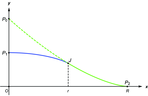
Throughout this paper we denote by the function
| (2.2) |
and by the function
In Figure 2.1, the solid curve represents the graph of on , while the half-dashed and half-solid curve represents the graph of on .
Lemma 2.1.
For any and all , if then
| (2.3) |
where
Proof.
Lemma 2.2.
There exists a constant such that for any and all sufficiently large if then
| (2.4) |
where
| (2.5) |
with determined by the equation .
Proof.
Denote
For sufficiently large we apply to all four factors in (2.1) Olver’s asymptotic expansions of Bessel functions of large order (see [1, p. 368] or Olver’s original paper [18]; for the convenience of the readers we put those formulas in the appendix). The and appearing in the asymptotics are both negative and determined by (A.8). They satisfy the following size estimates:
and
whenever is sufficiently large. Indeed, the first estimate follows from (with to be determined below) while the second one follows from (A.10) and .
Then
| (2.6) |
with the error being an expression involving the Airy functions of the first and second kind.
Since
and are both of size while and of size (see [1, p. 448–449]), by using the well-known asymptotics for the Airy functions (see the appendix) and the angle difference formula for the sine, the terms in brackets in (2.6) become
where
By (A.10), if is a sufficiently small constant then . Noticing the definition of and , we then get (2.4) and (2.5). ∎
Lemma 2.3.
There exists a strictly decreasing real-valued function such that , , , and the image of is a bounded interval. For any and all sufficiently large if then
| (2.7) |
where is determined by the equation and
| (2.8) |
Proof.
Notice that if then
for some fixed constant whenever is sufficiently large. Denote
Applying (A.1) and (A.2) to and respectively and Lemma A.1 to both and yields
| (2.9) | ||||
| (2.10) |
where
To get the bound of , we used the fact that for large
| (2.11) |
(see §2.2 in [19, p. 395]) and noticed that .
In order to use the angle sum formula for the sine to simplify (2.9) and (2.10) we define an angle function as follows
where and () is the th zero of the equation . Then the terms in brackets in (2.9) and (2.10) become
| (2.12) |
Notice that if then (A.11) implies
Define a real-valued function by
By rewriting (2.12) with this and the function , we get (2.7) and (2.8).
One can easily check, after checking that is always negative, that does satisfy those properties claimed in the statement of the lemma. For non-positive , follows trivially from the formula
in whose calculation we have used the 10.4.10 in [1, p. 446]. To prove the inequality for positive , it suffices to show that
This follows from the fact that the left hand side is an increasing function of (see §2.4 in [19, p. 397] and §7.3 in [19, p. 342] or §13.74 [21, P.446]) and (2.11). Since as , its image should be a bounded interval. ∎
Remark 2.4.
It follows from the 10.4.78 in [1, p. 449] that for large
Lemma 2.5.
For all , at any positive zero of ,
In particular, .
Proof.
Lemma 2.6.
For any and all sufficiently large if then
| (2.13) |
where and
| (2.14) |
If we further assume that , then
| (2.15) |
where
| (2.16) |
Remark 2.7.
Proof of Lemma 2.6.
As in the proof of Lemma 2.2, we denote
Since the , determined by (A.8), is negative such that
Meanwhile, since the , determined by (A.9), is positive such that
whenever is sufficiently large.
With the estimate
applying Olver’s asymptotic expansions (A.6) and (A.7) and asymptotics for the Airy functions (the 10.4.59, 10.4.61, 10.4.63, and 10.4.66 in [1]) yields
and
Hence is always negative and
Therefore
| (2.17) |
We can now collect all previous lemmas and give a description of zeros of for large .
Theorem 2.8.
There exists a constant such that for any and all sufficiently large the positive zeros of , , satisfy the following:
-
(1)
if then
(2.18) -
(2)
if then
(2.19) with determined by the equation ;
- (3)
-
(4)
if then
(2.21) where
Proof.
The rough idea of this proof is to apply to the intermediate value theorem in the interval for any sufficiently large integer and then J. Cochran’s result of the number of zeros within such an interval (see [4]).
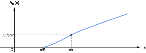
We will study zeros of only in for any sufficiently large integer since Lemma 2.5 tells us that there is no zeros . Inspired by the asymptotics obtained in this section, the study will be done via discussing the values of †††This notation will be used through the rest of this section. on the chosen interval (see Figure 2.2 for an example of the graph of ).
We observe that is a continuous and strictly increasing function that maps onto . Therefore for each integer there exists an interval such that maps to bijectively. It is obvious that these intervals ’s are disjointly located one by one as increases.
We claim that if is sufficiently large then for each
| (2.22) |
If this is true, the intermediate value theorem ensures the existence of at least one zero of in each . Recall that there are exactly zeros of in (see [4]). Hence there exists one and only one zero in each , which must be by definition.
To verify (2.22) we take advantage of the asymptotics (2.3), (2.4), (2.7), (2.15) and (2.13). In all cases except the last one (when for a sufficiently large ), the verification is easy if we notice that
for any . In the last case when we use the asymptotics (2.13). The sign of depends on that of
| (2.23) |
As in the proof of Lemma 2.3, we denote by () the th zero of the equation . [19, P.405] gives that
with a crude estimate . Thus
| (2.24) |
Since oscillates around zero for positive and the intervals in (2.24) are disjoint for different ’s, the signs of (2.23) at and must be opposite whenever is sufficiently large, which in turn gives (2.22) in the last case.
We are now able to finish the proof of the theorem. For each zero , . If we apply to the left hand side either (2.3), (2.4), (2.7) or (2.15), and conclude that the factor involving the sine function and has to be zero. Since is always in the interval for any , applying the arcsine function immediately yields the desired asymptotics. If we use the fact that to get a crude estimate . ∎
For small we have the following.
Theorem 2.9.
For any there exists a constant such that if and then the positive zero of satisfies
| (2.25) |
Proof.
If and for a sufficiently large constant then Lemma 2.1 (with ) gives a factorization (2.3) of with . By using such a factorization we study on the interval
| (2.26) |
which is a subset of if is sufficiently large. As in the proof of Theorem 2.8, we then study the function on a subinterval of (2.26), denoted by , with . Such a subset indeed exists if is sufficiently large since .
It is easy to see that . By the intermediate value theorem there exists at least one zero of in , which must be since there exists exactly one zero in the interval (2.26) if is sufficiently large (due to the fact that there are exactly zeros of in for sufficiently large integer (see [4])). Thus
Applying the arcsine function yields the desired result. ∎
Corollary 2.10.
Given any sufficiently large integer and , for all ’s that are greater than we have
Furthermore, if then the dependence of the implicit constant on can be removed.
For any if and is sufficiently large then
Proof.
If , a straightforward computation shows that if then
if then
For all sufficiently large the desired results follow from Theorem 2.8, the mean value theorem and the above first derivatives. For any and , we observe that if is sufficiently large (depending on ) then . We can then derive the desired result similarly with Theorem 2.8 replaced by Theorem 2.9.
The case follows trivially from Theorem 2.9. ∎
Corollary 2.11.
Remark 2.12.
These bounds are all as small as we want if we choose or properly large. It is quite obvious to observe this except (perhaps) for the second bound. As to that, we just need to notice (2.27) below and the corresponding range of , namely .
Proof of Corollary 2.11.
Let be the function homogeneous of degree which satisfies on the graph of . By implicit differentiation, we have
and
where is determined by , that is, is the intersection point of the graph of and the line segment connecting the origin and the point . Analyzing the sizes of the above derivatives yields
Lemma 2.13.
Following the above notations, we have that if for a sufficiently small constant then
otherwise
We also have . In particular, if then
By Theorem 2.8 and 2.9, Corollary 2.11 and Lemma 2.13, we have the following approximations of zeros.
Corollary 2.14.
There exists a constant such that for any there exists a such that if then the positive zeros of , , satisfy
| (2.29) |
where
| (2.30) |
where is the function appearing in Lemma 2.3 with determined by the equation , and
If there exists a such that if then (2.29) holds with
| (2.31) |
and
Proof.
If then for sufficiently large . By using (2.18)–(2.20) and the monotonicity of , we have
which, by Lemma 2.13, ensures that . The (2.29) with then follows from (2.18)–(2.20), the mean value theorem and Corollary 2.11.
3. Spectrum counting to lattice counting
Consider the Dirichlet Laplacian operator on the planar annulus . Using the standard separation of variables, we know that its spectrum contains exactly the numbers , , , defined at the beginning of Section 2. We also know that in the spectrum each appears twice for every fixed and only once if . If we define for any negative integer , then the spectrum counting function defined by (1.1) becomes
Recall that we define in Corollary 2.14 (with the and appearing there fixed) the amount of translation for , , namely, (2.30) and (2.31). We now extend its definition to by letting be if and if . In view of the multiplicity of the spectrum and Corollary 2.14, each , , corresponds to a unique point .
Denote by the closed domain symmetric about the -axis and in the first quadrant bounded by the graph of and the -axis. See the shaded area in Figure 3.1. Define a lattice counting function by
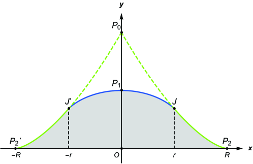
Then one can transfer the spectrum counting problem to a lattice counting problem via the following result. In its proof we essentially follow the treatment for “the boundary parts” in [6, Theorem 3.1].
Proposition 3.1.
There exists a constant such that
| (3.1) |
Proof.
To study we would like to use the approximations of ’s given by Corollary 2.14. We need to assume that is sufficiently large, however, we will not emphasize this explicitly in the following argument. This treatment will not cause any problem; after all, it will produce at most an error, which is much less than the error term in (3.1).
For , let
and
Then
| (3.2) |
Hence we only need to consider points satisfying .
We next use Lemma 2.13 and Corollary 2.14 to obtain bounds of . We discuss in several cases depending on the size of .
If then
| (3.3) |
Indeed, in this case we have . This, together with Theorem 2.8, leads to
which implies that is close to and thus . Therefore . Using the estimate of we get (3.3).
If then a similar argument as above shows that and
If for a sufficiently large constant (to be determined below) then
| (3.4) |
for some constant . Indeed, let us fix arbitrarily an element belonging to the set in (3.2), hence the point is contained in a tubular neighborhood of of width much less than (see Remark 2.12). Since is continuous at the point and , as the tubular neighborhood (mentioned above) between and is close to a parallelogram. A simple geometric argument ensures that if is a sufficiently large constant then . As a result,
| (3.5) |
On the other hand side we observe, as a consequence of Theorem 2.8 and the monotonicity of , that if then
which contradicts with (3.5). Therefore and can only be either or , both of which are of size since . We then readily get (3.4).
If then the trivial estimate yields that
If then
| (3.6) |
for some constant . Since the proof is almost the same as that of (3.4), let us be brief. We still fix arbitrarily an element belonging to the set in (3.2). A geometric argument shows that . Thus
However, if then
which is impossible. Hence and can be in the form of , or . In fact, we further observe that if is sufficiently small then is sufficiently large and must be , as a consequence of Theorem 2.8 and 2.9. To conclude the proof of (3.6), we only need to notice that no matter in which form the is, it is always of size .
If , by using exactly the same argument as above we get
| (3.7) | |||
for some constant .
To conclude, summing the above bounds of over and using the symmetry between positive and negative ’s and the bound (3.7) yields the desired inequality. ∎
counts the number of lattice points (under various translations) in . This feature brings us some obstacles in its estimation. To overcome this difficulty we move every point to to obtain an uniformity in translation, and then study the relatively standard lattice counting function
| (3.8) |
Here the superscript “u” represents the uniformity in translation. Of course such a transformation from to will cause a difference. To quantify that we need to count the number of lattice points in a band of length and width . (This will be clear in the proof of the next proposition.)
For let us define a band on by
and the number of in the band by
| (3.9) |
One would expect the error term to be much smaller than the linear term since heuristically the number of lattice points inside a large planar domain is asymptotically equal to the area of the domain with an error term that is not too bad if the curvature involved does not vanish. We will estimate in the next section.
With defined as above we have
Proposition 3.2.
Proof.
In view of the definition of , moving the points down to can possibly get some of these points in the domain but no points out. Hence the difference between and is equal to twice (due to the symmetry) the number of points in the band that are moved in the domain . There are three types of points in this band:
-
(1)
’s, which correspond to the case and definitely get in ;
-
(2)
’s with , which may get in ;
-
(3)
’s, which correspond to the case and are not moved.
Concerning these three types of points, one key observation is that the points of the first type are all above the line passing through and (see Figure 3.1) while the points of the third type are all below. This is because of the facts that if then and if then . We only prove the former fact while the latter one’s proof is similar. Indeed, by Theorem 2.8 and the monotonicity of if then
which is greater than since . If similarly we have
By the mean value theorem and a straightforward computation of , we have
Combining the last two inequalities yields the desired one.
Another key observation is that any point of the second type in the band is such that for some large constant . Indeed, by Corollary 2.14, if then
Plugging this formula of into the above inequality of yields the desired range of .
As a result, the points in the band are only of the first type, which definitely get in . By (3.9) its number is equal to . Some of the points with may get in . Its number is of size . The points in are only of the third type and not moved. To sum up, the number of points in the band that are moved in the domain is . This finishes the proof. ∎
Theorem 3.3.
with and .
Thus we have transferred the study of to those of and , which will be done in the following section.
4. Lattice Counting and Proof of Theorem 1.1
In this section we study the two associated lattice point problems, and , defined in (3.8) and (3.9) respectively. Theorem 1.1 follows directly from Theorem 3.3, Theorem 4.1 and Corollary 4.5.
Recall that
denotes the number of points in the shifted lattice which lie in . The domain , defined in Section 3 (see Figure 3.1), has an area
Theorem 4.1.
Let . If the boundary curve of has a tangent in with rational slope (i.e. ), then
where
| (4.1) |
In case of an irrational slope the asymptotics remains true with the much weaker error term .
Remark 4.2.
If the tangent in J has rational slope (this includes the case ) the error term is of the same quality as the best published result in the circle problem due to Huxley [9]. The linear term can be explained as follows. To every lattice point one can associate an axes parallel square of volume 1 with center in the lattice point. Every such square contributes to the volume of its intersection with . The points with are not counted in , but contribute to the volume .
Since the boundary of contains points with infinite curvature (the points , and , ) standard results are not directly applicable. But see [17] for a lattice point counting problem in a non-convex domains with cusps and unbounded curvature. Our proof uses the following deep result of M.N. Huxley.
Proposition 4.3.
Let be real parameters and a three times continuously differentiable function satisfying
for . Denote by the row-of-teeth function and by , the constants defined in (4.1). Then there is a constant which depends only on and , such that
provided that
| (4.2) |
Proof.
This is Case A of Proposition 3 in [9].∎
Remark 4.4.
In contrast to van der Corput’s classical estimate (4.11) the proposition uses a condition on the first derivative. In our application becomes large if we count lattice points near to the boundary point along lines parallel to the axes. To avoid this we count them on lines parallel to the tangent. This is only possible if the tangent in has rational slope.
Proof of Theorem 4.1.
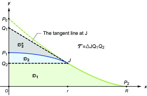
Slightly more general we count points in the shifted lattice with . The number is twice the number of shifted lattice points in the positive quadrant, if points on the -axis are counted with weight 1/2. Divide in domains
See Figure 4.1 for these domains.
The rational case of Theorem 4.1 follows if we prove that
| (4.3) | ||||
| (4.4) |
where describes the contribution of the line segment separating from . While (4.3) is true in general, we prove (4.4) in the irrational case only with the weaker error term .
In we count lattice points along lines parallel to the -axis. Denote by the inverse function of restricted to . Since points on the -axis are counted with weight 1/2, and , one finds
Euler’s summation formula
is used to calculate the first sum. The first integral gives the main term
By the second mean value theorem and Lemma 4.6 the second integral is bounded by
Together we obtain
For the -sum is estimated trivially. This contributes to . The remaining sum is divided in sums of the form
| (4.5) |
where . To apply Proposition 4.3 set
and . By Lemma 4.6 for and . The condition (4.2) is satisfied since . This yields the bound for (4.5). Summing over gives (4.3). Note that this already completes the treatment of the special case .
If we have to deal with . First we assume that the tangent in has rational slope. Hence with , relatively prime. The number of shifted lattice points in is equal to the number of shifted lattice points in the triangle minus the number of shifted lattice points in , where
In case of and it is easier to count points on the -axis with full weight. Then
| (4.6) |
In we count points along the lines , . Note that contains points of the shifted lattice if and only if is an integer. The line intersects the lower boundary curve of between and in a unique point if , where
Define a function by writing the -coordinate of the intersection point as . The defining equation of reads
| (4.7) |
The strictly increasing function maps to . For every choose such that . If the lattice points on are the points with , . Hence the number of shifted lattice points in is equal to the number of integers such that . Since the number of integers in is this number is
This yields
| (4.8) |
with
Using the relation
| (4.9) |
simplifies to
Euler’s summation formula applied to the first sum in (4.8) yields
By the second mean value theorem, Lemma 4.7 and (4.15) the last integral is bounded by
In the inner sum of we estimate the terms with trivially. The remaining sum is divided in sums of the form
where , and
with . By Lemma 4.7 for . The condition (4.2) of Proposition 4.3 is satisfied since . This yields the bound . Summing over gives . Together this proves
| (4.10) |
Corollary 4.5.
Proof.
In we count unshifted lattice points. The number of unshifted lattice points in is given by (4.4) with . Thus in the rational case (4.12) is equivalent to
| (4.13) |
where denotes the number of unshifted lattice points in with
Repeating the proof of (4.4) with this slightly modified domain one obtains (4.13). The case of irrational slope is even easier. ∎
Lemma 4.6.
Let . The inverse function of restricted to satisfies for j=1,2,3
Proof.
For the function satisfies
and, with the positive and bounded function ,
Furthermore is positive with
This proves
Set . Then . For the inverse function one obtains
∎
Lemma 4.7.
Let . The function defined in (4.7) satisfies for j=1,2,3
Appendix A Some asymptotics
For any and , if the Bessel functions have the asymptotics
| (A.1) |
and
| (A.2) |
where is defined by (2.2).
We first study the integral . The phase function has only one critical point in . Applying the method of stationary phase in a sufficiently small neighborhood of yields the contribution
| (A.3) |
To study the contribution of the domain away from we use integration by parts twice. The real part contributes at most while the imaginary part is equal to
| (A.4) |
We then immediately get (A.1) by taking the real part of .
It remains to study . If , by using a substitution and integration by parts twice, we get
If then
| (A.5) |
Indeed, by changing variables we have
where
Therefore, by the mean value theorem,
After using the Gamma function to simplify the right hand side, we get a convergent geometric series which is . This proves (A.5).
Repeating the above argument for (A.5) (even for small ) yields
Finally, combining (A.3), (A.4), and the above asymptotics of leads to (A.2) readily. This finishes the proof.
Furthermore, we use Olver’s uniform asymptotic expansions of Bessel functions of large order (see [1, p. 368] or [18]):
| (A.6) |
and
| (A.7) |
where is given by
| (A.8) |
or
| (A.9) |
Here the branches are chosen so that is real when is positive. and denotes the Airy functions of first and second kind. For the definitions and sizes of the coefficients ’s and ’s see [1, p. 368–369], especially . It is easy to check the following expansions of (A.8) and (A.9). If then
| (A.10) |
If then
| (A.11) |
As a consequence of Olver’s asymptotics we obtain the following analogue of the 9.3.4 in [1, p. 366].
Lemma A.1.
For any and all sufficiently large ,
-
(1)
if then
-
(2)
if then
Proof.
We may assume that for a large constant , otherwise all desired formulas follow from 9.3.4 in [1, p. 366] since and if .
Let us consider the case . Set . By (A.6) we have
where , determined by (A.9), is positive and satisfies by (A.11)
Thus
| (A.12) |
Since it is known ([1, p. 448]) that for large
and
we have
and, by the mean value theorem,
Collecting the above three estimates and plugging them into the above formula of gives the desired formula of in the case . Almost the same argument gives the formula of .
In the case we again use the asymptotics (A.6) and (A.7) with . The corresponding , determined by (A.8), is negative and satisfies by (A.10)
which leads to (A.12). Since and (see [1, p. 448–449]), we get
and
Collecting these estimates and plugging them into (A.6) gives the desired formula of in the case . A similar argument gives the formula of . ∎
Finally, we collect two well-known asymptotic formulas for the Airy functions (see for example [1, p. 448–449]). For
and
References
- [1] Abramowitz, M. and Stegun, I. A., Handbook of mathematical functions with formulas, graphs, and mathematical tables, National Bureau of Standards Applied Mathematics Series, 55, For sale by the Superintendent of Documents, U.S. Government Printing Office, Washington, D.C., 1964.
- [2] Bobkov, V., Asymptotic relation for zeros of cross-product of Bessel functions and applications, J. Math. Anal. Appl. 472, 1078–1092, 2019.
- [3] Bourgain, J. and Watt, N., Mean square of zeta function, circle problem and divisor problem revisited, arXiv:1709.04340.
- [4] Cochran, J. A., Remarks on the zeros of cross-product Bessel functions, J. Soc. Indust. Appl. Math. 12, 580–587, 1964.
- [5] Cochran, J. A., The analyticity of cross-product Bessel function zeros, Proc. Cambridge Philos. Soc. 62, 215–226, 1966.
- [6] Colin de Verdière, Y., On the remainder in the Weyl formula for the Euclidean disk, Séminaire de théorie spectrale et géométrie 29, 1–-13, 2010–2011.
- [7] Duistermaat, J. and Guillemin, V.,The spectrum of positive elliptic operators and periodic bicharacteristics, Invent. Math. 29, 39–79, 1975.
- [8] Guo, J., Wang, W. and Wang, Z., An improved remainder estimate in the Weyl formula for the planar disk, J. Fourier Anal. Appl., to appear, available at https://doi.org/10.1007/s00041-018-9637-z.
- [9] Huxley, M. N., Exponential sums and lattice points. III, Proc. London Math. Soc. (3) 87, 591–609, 2003.
- [10] Ivrii, V., The second term of the spectral asymptotics for a Laplace-Beltrami operator on manifolds with boundary (Russian), Funct. Anal. Appl. 14, 25–34, 1980.
- [11] Kline, M., Some Bessel equations and their application to guide and cavity theory, J. Math. Physics 27, 37–48, 1948.
- [12] Kuznetsov, N. V. and Fedosov, B. V., An asymptotic formula for eigenvalues of a circular membrane, Differ. Uravn. 1, 1682–1685, 1965.
- [13] Lazutkin, V. F. and Terman, D. Ya., On the estimate of the remainder term in a formula of H. Weyl (Russian), Funct. Anal. Appl. 15, 299–300, 1982.
- [14] McCann, R. C., Lower bounds for the zeros of Bessel functions, Proc. Amer. Math. Soc. 64, 101–103, 1977.
- [15] McMahon, J., On the roots of the Bessel and certain related functions, Ann. of Math. 9, 23–30, 1894/95.
- [16] Melrose, R. B., Weyl’s conjecture for manifolds with concave boundary, Geometry of the Laplace operator (Proc. Sympos. Pure Math., Univ. Hawaii, Honolulu, Hawaii, 1979), pp. 257–274, Proc. Sympos. Pure Math. XXXVI, Amer. Math. Soc., Providence, R.I., 1980.
- [17] Nowak, W. G., A nonconvex generalization of the circle problem, J. Reine Angew. Math. 314, 136–145, 1980.
- [18] Olver, F. W. J., The asymptotic expansion of Bessel functions of large order, Philos. Trans. Roy. Soc. London. Ser. A. 247, 328–368, 1954.
- [19] Olver, F. W. J., Asymptotics and Special Functions, Academic Press, New York, 1974; reprinted by A. K. Peters, Wellesley, MA, 1997.
- [20] Van der Corput, J. G., Zahlentheoretische Abschätzungen mit Anwendung auf Gitterpunktprobleme (German), Math. Z. 17, 250–259, 1923.
- [21] Watson, G. N., A treatise on the theory of Bessel functions, Reprint of the second (1944) edition, Cambridge Mathematical Library, Cambridge University Press, Cambridge, 1995.
- [22] Weyl, H., Das asymptotische Verteilungsgesetz der Eigenwerte linearer partieller Differentialgleichungen (mit einer Anwendung auf die Theorie der Hohlraumstrahlung). (German), Math. Ann 71, 441–479, 1912.
- [23] Weyl, H., Über die Randwertaufgabe der Strahlungstheorie und asymptotische Spektralgeometrie. (German), J. Reine Angew. Math 143, 177–202, 1913.
- [24] Willis, D. M., A property of the zeros of a cross-product of Bessel functions, Proc. Cambridge Philos. Soc. 61, 425–428, 1965.