The Abundance and Structure of Subhaloes near the Free Streaming Scale and Their Impact on Indirect Dark Matter Searches

Abstract

The free streaming motion of dark matter particles imprints a cutoff in the matter power spectrum and set the scale of the smallest dark matter halo. Recent cosmological $N$-body simulations have shown that the central density cusp is much steeper in haloes near the free streaming scale than in more massive haloes. Here, we study the abundance and structure of subhaloes near the free streaming scale at very high redshift using a suite of unprecedentedly large cosmological $N$-body simulations, over a wide range of the host halo mass. The subhalo abundance is suppressed strongly below the free streaming scale, but the ratio between the subhalo mass function in the cutoff and no cutoff simulations is well fitted by a single correction function regardless of the host halo mass and the redshift. In subhaloes, the central slopes are considerably shallower than in field haloes, however, are still steeper than that of the NFW profile. Contrary, the concentrations are significantly larger in subhaloes than haloes and depend on the subhalo mass. We compare two methods to extrapolate the mass-concentration relation of haloes and subhaloes to z=0 and provide a new simple fitting function for subhaloes, based on a suite of large cosmological $N$-body simulations. Finally, we estimate the annihilation boost factor of a Milky-Way sized halo to be between 1.8 and 6.2.

1 Introduction

The smallest dark matter haloes are the first gravitationally collapsed structures in the Universe according to the hierarchical structure formation scenario. The free streaming motion of particles imprints a cutoff in the matter power spectrum at the initial stage of the Universe and determines the size of the smallest haloes. If dark matter consists of Weakly Interacting Massive Particle (WIMP) of mass approximately 100 Ge,V their mass has been estimated to be near Earth-mass, $10^{-12}\mbox{\scriptsize--}10^{-3}$$\rm M_{\odot}$ (e.g., Zybin et al., 1999; Hofmann et al., 2001; Berezinsky et al., 2003; Green et al., 2004; Loeb & Zaldarriaga, 2005; Bertschinger, 2006; Profumo et al., 2006; Berezinsky et al., 2008; Diamanti et al., 2015).

In this decade, the density profiles of haloes near the free streaming scale have been studied by means of cosmological $N$-body simulations (Diemand et al., 2005; Ishiyama et al., 2010; Anderhalden & Diemand, 2013; Ishiyama, 2014; Angulo et al., 2017; Delos et al., 2019), merger simulations (Ogiya et al., 2016; Angulo et al., 2017), cold collapse simulations (Ogiya & Hahn, 2018), and idealized tidal evolution simulations (Delos, 2019). Ishiyama et al. (2010) found that the central density cusps are considerably steeper in microhaloes than more massive haloes and are well described by $\rho(r)\propto r^{-1.5}$. These results are supported by other similar cosmological simulations using different simulation codes (Anderhalden & Diemand, 2013; Angulo et al., 2017) and are reproduced by cold collapse simulations (Ogiya & Hahn, 2018). Ishiyama (2014) (hereafter I14) extended these results with better statistics and found that the cusp slope gradually becomes shallower with increasing halo mass, as a result of major merger processes (see also Ogiya et al., 2016; Angulo et al., 2017). Similar profiles are obtained in warm dark matter simulations (Polisensky & Ricotti, 2015), in which the cutoff in the matter power spectrum is also imposed although its corresponding mass scale is much larger than that of microhaloes. Steeper cusps are also observed in recent simulations of ultracompact minihaloes (Gosenca et al., 2017; Delos et al., 2018b, a).

Such steep cusps may have a significant effect on dark matter searches. There are a variety of subjects such as gravitational lensing (Chen & Koushiappas, 2010; Erickcek & Law, 2011; Van Tilburg et al., 2018), Gravitational Waves (Bird et al., 2016), Galactic tidal fluctuations (Peñarrubia, 2018), gravitational perturbations on the Solar system (González-Morales et al., 2013), pulsar timing arrays (Ishiyama et al., 2010; Baghram et al., 2011; Kashiyama & Oguri, 2018) and indirect detection experiments (e.g., Berezinsky et al. 2003; Koushiappas et al. 2004; Koushiappas 2006; Goerdt et al. 2007; Diemand et al. 2007; Ando et al. 2008; Ishiyama 2014; Bartels & Ando 2015; Fornasa & Sánchez-Conde 2015; Anderson et al. 2016; Marchegiani & Colafrancesco 2016; Hütten et al. 2016, 2018; Hooper & Witte 2017; Moliné et al. 2017; Stref & Lavalle 2017; Hiroshima et al. 2018; Ando et al. 2019b; Karwin et al. 2019, and see also a recent review by Ando et al. 2019a). I14 showed that the steeper inner cusps of haloes near the free streaming scale can increase the dark matter annihilation luminosity of a Milky-Way sized halo between 12 % to 67 %, compared with the case we assume the NFW density profile (Navarro et al., 1997) and an empirical mass-concentration relation proposed by Sánchez-Conde & Prada (2014). However, this estimation relies on density profiles seen in field haloes, not subhaloes. To make a more robust estimation, quantifying the structures of subhaloes near the free streaming scale is necessary.

Not the density structure but the abundance of microhaloes in the Milky-Way halo are crucial for the annihilation signal. Analytic studies and cosmological simulations have suggested that the subhalo mass function is expressed as $dn/dm\propto m^{\zeta}$, with the slope $\zeta$ of $-(2\mbox{\scriptsize--}1.8)$ (e.g., Hiroshima et al., 2018), although there is no consensus. The cutoff in the matter power spectrum should suppress the number of subhaloes near the free streaming scale, which should weaken the annihilation signal. However, the shape of the mass function near the free streaming scale is not understood well, in particular, for the case of WIMP dark matter.

We address these questions by large and high resolution cosmological $N$-body simulations. This paper presents the first challenge to reveal the structure of subhaloes near the free streaming scale. To reliably study the statistics of these subhaloes, we conducted huge simulations with sufficient spatial volumes. § 2 describes our simulation method and its setup. The mass function, density profiles, and concentrations of subhaloes near the free streaming are presented in § 3. The contributions of these haloes to gamma-ray signals by WIMP self-annihilation is discussed in § 4. The results are summarized in § 5.

2 Initial Conditions and Numerical Method

Table 1: Parameters of a suite of cosmological $N$-body simulations performed in this work. Those of three simulations conducted in I14 are also shown for the comparison. Here, $N$, $L$, $\varepsilon$, $M_{\rm total}$, and $m_{\rm p}$ are the total number of particles, box length, softening length, total mass in the box, and particle mass resolution, respectively. The final redshift when the simulations are terminate is $z=32$.

Name	$N$	$L($pc$)$	$\varepsilon($pc$)$	$M_{\rm total}$ ($\rm M_{\odot}$)	$m_{\rm p}$ ($\rm M_{\odot}$)	cutoff	reference
A_N8192L800	$8192^{3}$	800.0	$2.0\times 10^{-4}$	20.37	$3.7\times 10^{-11}$	w/	this work
A_N4096L400	$4096^{3}$	400.0	$2.0\times 10^{-4}$	2.35	$3.4\times 10^{-11}$	w/	Ishiyama (2014)
A_N4096L200	$4096^{3}$	200.0	$1.0\times 10^{-4}$	0.30	$4.3\times 10^{-12}$	w/	Ishiyama (2014)
B_N4096L400	$4096^{3}$	400.0	$2.0\times 10^{-4}$	2.55	$3.7\times 10^{-11}$	w/o	this work
B_N2048L200	$2048^{3}$	200.0	$2.0\times 10^{-4}$	0.30	$3.4\times 10^{-11}$	w/o	Ishiyama (2014)

Table 2: Same as Table 1. Here, $z_{\rm fin}$ is the redshift when the simulation is terminated. These five simulations do not account the cutoff in the matter power spectrum.

Name	$N$	$L(h^{-1}\rm Mpc)$	$\varepsilon(h^{-1}\rm kpc)$	$M_{\rm total}(h^{-1}\rm M_{\odot})$	$m_{\rm p}(h^{-1}\rm M_{\odot})$	$z_{\rm fin}$	reference
$\nu^{2}$GC-S	$2048^{3}$	280.0	$4.28$	$1.89\times 10^{18}$	$2.20\times 10^{8}$	0.0	Ishiyama et al. (2015)
$\nu^{2}$GC-H2	$2048^{3}$	70.0	$1.07$	$2.95\times 10^{16}$	$3.44\times 10^{6}$	0.0	Ishiyama et al. (2015)
Phi-0	$2048^{3}$	8.0	$0.12$	$4.40\times 10^{13}$	$5.13\times 10^{3}$	0.0	Ishiyama et al. (2016)
Phi-1	$2048^{3}$	32.0	$0.48$	$2.82\times 10^{15}$	$3.28\times 10^{5}$	0.0	this work
Phi-2	$2048^{3}$	1.0	$7.5\times 10^{-3}$	$8.60\times 10^{10}$	$10.0$	5.0	this work

To follow the formation and evolution of haloes and subhaloes near the free streaming scale, we conducted two ultralarge cosmological $N$-body simulations. The matter power spectrum in the simulation denoted A_N8192L800 accounted the cutoff imposed by the free motion of dark matter particles (Green et al., 2004). The cutoff scale is nearly earth-mass, $10^{-6}$$\rm M_{\odot}$. The other simulation denoted B_N4096L400 ignored the effect of the free motion. The cosmological parameters are $\Omega_{0}=0.31$, $\rm\lambda_{0}=0.69$, $h=0.68$, $n_{\rm s}=0.96$, and $\sigma_{8}=0.83$, which are consistent with an observation of the cosmic microwave background obtained by the Planck satellite (Planck Collaboration et al., 2014, 2016, 2018). The initial conditions were generated by a first-order Zeldovich approximation at $z=400$. Note that the power spectrum near the cutoff scale can be increased in early matter dominated era (Erickcek, 2015), which we do not consider here.

In the simulations, A_N8192L800 and B_N4096L400, the gravitational evolution of $8192^{3}$ and $4096^{3}$ particles in comoving boxes of side length 800 pc and 400 pc were calculated, respectively. The particle masses of both simulations are $3.7\times 10^{-11}M_{\odot}$, comparable to those of I14. The gravitational softening length is $2.0\times 10^{-4}$ pc. The parameters of the two simulations and our earlier ones (Ishiyama, 2014) are listed in Table 1.

The gravitational evolution was followed by a massively parallel TreePM code, GreeM (Ishiyama et al., 2009; Ishiyama et al., 2012) on the K computer at the RIKEN Advanced Institute for Computational Science, Aterui and Aterui II supercomputer at Center for Computational Astrophysics, CfCA, of National Astronomical Observatory of Japan. The evaluation of the tree force was accelerated by the Phantom-GRAPE software (Nitadori et al., 2006; Tanikawa et al., 2012, 2013; Yoshikawa & Tanikawa, 2018) with support for the HPC-ACE architecture of the K computer. These simulations were terminated at $z=32$.

Haloes were identified by the spherical overdensity method (Lacey & Cole, 1994). To calculate the virial mass of a halo $M_{\rm vir}$, we used the overdensity, $\Delta(z)=18\pi^{2}+82x-39x^{2}$ times the critical density in the Universe, where $x\equiv\Omega(z)-1$, based on the spherical collapse model (Bryan & Norman, 1998). The most massive haloes identified in A_N8192L800 and B_N4096L400 simulations contain 796,727,804 and 504,029,713 particles, corresponding $2.95\times 10^{-2}$$\rm M_{\odot}$ and $1.87\times 10^{-2}$$\rm M_{\odot}$, respectively. Subhaloes were identified by ROCKSTAR phase space halo/subhalo finder (Behroozi et al., 2013). The total number of haloes and subhaloes with masses larger than $10^{-6}$$\rm M_{\odot}$ are 32,907 and 22,936 for the A_N8192L800, and 20,915 and 3,987 for the B_N4096L400 at $z=32$.

To compare the structures of haloes and subhaloes near the free streaming scale with those of more massive haloes, we used three simulations taken from Ishiyama et al. (2015, 2016); Makiya et al. (2016), and conducted two new simulations. These five simulations do not account the cutoff in the matter power spectrum. The parameters of these simulations are summarized in Table 2.

To generate the initial conditions for the $\nu^{2}$GC-S, $\nu^{2}$GC-H2, and Phi-0 simulations, we used a publicly available code, 2LPTic. The initial conditions for the Phi-1 and Phi-2 simulations were generated by a publicly available code, MUSIC (Hahn & Abel, 2011). Both codes adopt second-order Lagrangian perturbation theory (e.g., Crocce et al., 2006). The other numerical method and cosmological parameters used in these simulations are the same as described above. The Rockstar catalogues and consistent merger trees of the $\nu^{2}$GC-S, $\nu^{2}$GC-H2, and Phi-1 simulations are publicly available at http://hpc.imit.chiba-u.jp/~ishiymtm/db.html.

3 Results

3.1 Subhalo Mass Function

We selected subhaloes found within the virial radius of their host haloes and calculated the subhalo mass function of each halo. To derive the proper average mass functions of haloes with vast mass distribution, we stacked the mass function of similar-mass haloes. Figure 1 shows the stacked subhalo mass functions of the simulations A_N8192L800 and B_N4096L400 for three different ranges of the host halo mass, $1.00\mbox{--}3.16\times 10^{-2}$$\rm M_{\odot}$, $1.00\mbox{--}3.16\times 10^{-3}$$\rm M_{\odot}$, and $1.00\mbox{--}3.16\times 10^{-4}$$\rm M_{\odot}$ at $z=32$ and 40. For the B_N4096L400 simulation, the stacked subhalo mass function of halo with the mass $1.00\mbox{--}3.16\times 10^{-2}$$\rm M_{\odot}$ is not displayed because of the absence of the host haloes.

The mass functions without the cutoff (B_N4096L400) show a nearly single power law except for the massive end, consistent with more massive host haloes and lower redshifts (e.g., Hiroshima et al., 2018). The mass functions with the cutoff (A_N8192L800) agree with those of the B_N4096L400 for the subhalo mass more massive than $\sim 5.0\times 10^{-6}$$\rm M_{\odot}$. For the less massive subhaloes, the slopes of mass functions $\zeta$ are gradually decreasing with decreasing subhalo mass differently from the B_N4096L400 simulation and are becoming flat at around $\sim 10^{-6}$$\rm M_{\odot}$, which corresponds to the cutoff scale. Interestingly, the slopes $\zeta$ are becoming steeper again below $\sim 10^{-7}$$\rm M_{\odot}$ due to artificial fragmentation as observed in simulations of warm dark matter (Wang & White, 2007; Schneider et al., 2013; Angulo et al., 2013).

These results are highlighted in Figure 2, which shows the ratio between the subhalo mass function with (A_N8192L800) and without (B_N4096L400) the cutoff at $z=32$, 40, and 50. As shown in Figure 1, the ratios are decreasing and flattening with decreasing subhalo mass, and show upturns at around $\sim 10^{-7}$$\rm M_{\odot}$ due to artificial fragmentation. The shapes of ratios agree well with each other regardless of the host halo mass and the redshift.

The ratio is well fitted by the correction function,

$${\rm f_{cor}}(M)=\frac{n_{\rm cut}}{n}=\frac{1}{2}\left(1+\frac{M_{1}}{M}\right)^{-1}\left[1+{\rm erf}\left(\ln\frac{M}{M_{2}}\right)\right],$$ (1)

where, $M_{1}=1.3\times 10^{-6}$, and $M_{2}=1.0\times 10^{-8}$, or $1.0\times 10^{-7}$$\rm M_{\odot}$. Hereafter, we call the former "correction function 1" and the later "correction function 2". To remove the influence of artificial fragmentation, dumping in the correction function is necessary around the free streaming scale. Because it is difficult to distinguish physical haloes from artificial fragmentation, we introduce two correction functions with different $M_{2}$ and compare the effect on the annihilation signal in § 4. From the nature of free streaming damping, this correction function should be valid for any mass scales more massive than $10^{-8}$$\rm M_{\odot}$ for the correction function 1 and $10^{-7}$$\rm M_{\odot}$ for the correction function 2.

This functional form is the same introduced in Angulo et al. (2013), which used it to fit the ratio of halo mass function in warm dark matter to cold dark matter simulations. This similarity seems to be a natural consequence because the physical origin of the dumping in the matter power spectrum is the same in both our simulations and warm dark matter simulations although there are more than ten orders of difference between their free streaming scales.

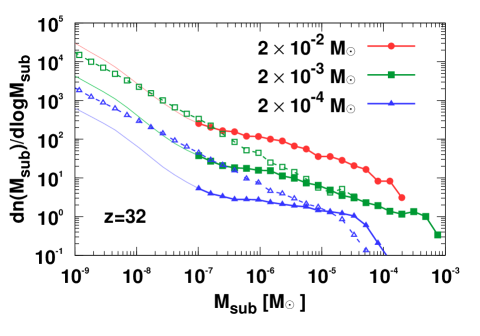
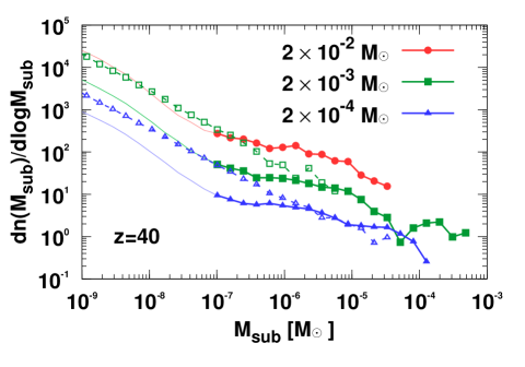
Figure 1: Stacked subhalo mass functions of haloes for three different mass bins, $2\times 10^{-2}$$\rm M_{\odot}$, $2\times 10^{-3}$$\rm M_{\odot}$, and $2\times 10^{-4}$$\rm M_{\odot}$, at $z=32$ (left) and 40 (right). Solid curves show the result of the simulation with the cutoff, A_N8192L800. Dashed curves show the result of the simulation without the cutoff, B_N4096L400. For subhaloes less massive than $\sim 5.0\times 10^{-6}$$\rm M_{\odot}$ in the A_N8192L800 simulation, the slopes of mass functions $\zeta$ are gradually decreasing with decreasing subhalo mass differently from the B_N4096L400 simulation and are becoming flat at around $\sim 10^{-6}$$\rm M_{\odot}$, which corresponds to the cutoff scale. The slopes $\zeta$ are becoming steeper again below $\sim 10^{-7}$$\rm M_{\odot}$ (displayed by thin curves) due to artificial fragmentation as observed in simulations of warm dark matter (Wang & White, 2007; Schneider et al., 2013; Angulo et al., 2013).

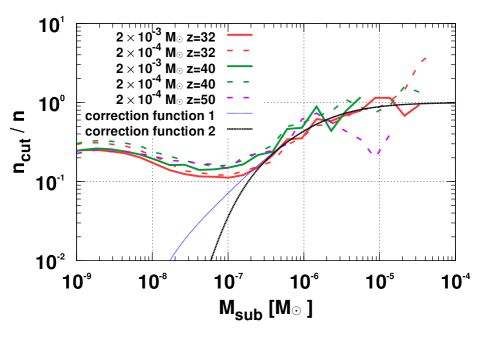
Figure 2: Effect of the cutoff in the matter power spectrum on the subhalo mass functions at $z=32$, 40, and 50: the ratio between the mass function with (A_N8192L800) and without (B_N4096L400) the cutoff. Thick and thin dotted curves show the two different correction functions to convert the mass function without the cutoff into with the cutoff as described in Equation (1).

From the independence of the subhalo mass function near the free streaming scale on the host halo mass and the redshift, the assumption should be justified that the shape of subhalo mass functions for more massive host haloes and lower redshifts should be similar to what we see in Figure 1. By extrapolating a subhalo mass function with a power law down to the smallest scale and multiplying the ratio shown in Figure 2 to it, we should be able to predict the mass function at an arbitrary redshift and of host halo mass, from the smallest to the largest scale under some assumptions for its normalization. This assumption is supported by analytic models (e.g., Hiroshima et al., 2018) that have found that the power law index of the subhalo mass function is in a rather narrow range between $-2$ and $-1.8$ with a vast range of halo/subhalo mass from $z=0$ to 5.

3.2 Subhalo Density Profiles

I14 have shown that the central density cusps are substantially steeper in haloes near the free streaming scale than more massive haloes when the cutoff is imposed in the matter power spectrum. A double power law function, given by

$$\rho(r)=\frac{\rm\rho_{0}}{(r/r_{\rm s})^{\alpha}(1+r/r_{\rm s})^{(3-\alpha)}},$$ (2)

fits density profiles better than NFW and Einasto profiles. The dependence of $\alpha$ and concentration parameter $c=r_{\rm vir}/r_{\rm s}$ on the halo mass is given in I14. The cusp slope gradually becomes shallower with increasing halo mass through major merger processes (see also Ogiya et al., 2016; Angulo et al., 2017). The concentration parameter slightly depends on the halo mass.

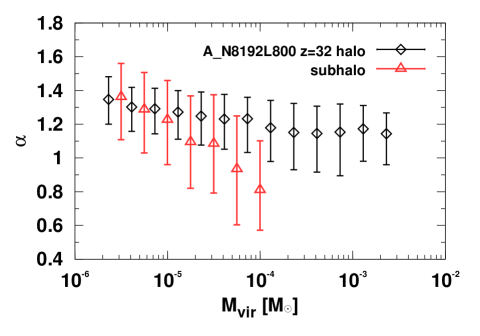
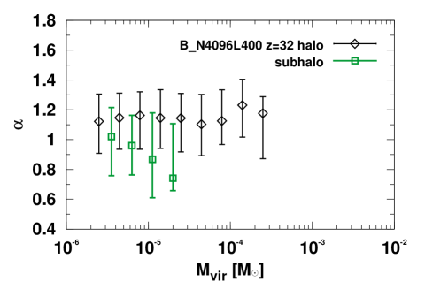
Figure 3: Slopes of the density profiles of field haloes and subhaloes $\alpha$ as a function of the virial mass $M_{\rm vir}$ at $z=32$, for the A_N8192L800 (left) and B_N4096L400 (right) simulations. Triangles, squares, and crosses are the median value in each mass bin. Whiskers give the first and third quantiles.

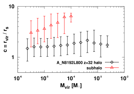
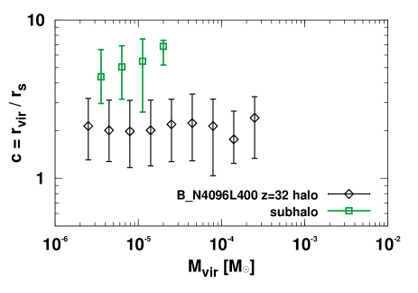
Figure 4: Concentrations of the density profiles of field haloes and subhaloes $r_{\rm vir}/r_{\rm s}$ as a function of the virial mass $M_{\rm vir}$ at $z=32$, for the A_N8192L800 (left) and B_N4096L400 (right) simulations. Triangles, squares, and crosses are the median value in each mass bin. Whiskers give the first and third quantiles.

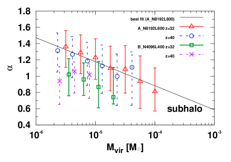
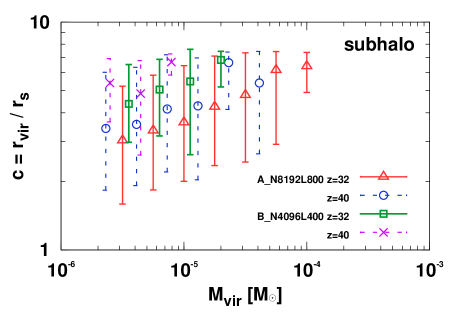
Figure 5: Evolution of the slopes (left) and concentrations (right) of subhaloes as a function of the virial mass $M_{\rm vir}$. Triangles, circles, squares, and crosses are the median value in each mass bin. Whiskers give the first and third quantiles.

These results are obtained in field haloes, not subhaloes. The structures of subhaloes should be different from field haloes because of tidal stripping. Cosmological simulations for more massive haloes have shown that subhaloes are more concentrated than field haloes (e.g., Ghigna et al., 2000; Bullock et al., 2001; Moliné et al., 2017). To estimate the annihilation signal more robustly, quantifying the structures of subhalo near the free streaming scale is necessary.

I14 has carefully performed resolution studies and have conservatively concluded that the inner density profile at 2% of their virial radius is well resolved for the haloes with masses more massive than $2\times 10^{-6}$$\rm M_{\odot}$ under the resolution of A_N4096L400 and B_N2048L200 simulations. Below this radius, numerical two-body relaxation becomes serious. The mass resolution and softening parameter of A_N8192L800 and B_N4096L400 simulations are comparable to those of the A_N4096L400 simulation, which is used in I14. Thus, we hereafter use the same criterion to quantify the density profiles of haloes and subhaloes in this study.

We calculated the spherically averaged radial density profile of each subhalo over the range $0.02\leq r/r_{\rm vir}\leq 1.0$, splitted into 32 logarithmically equal bins. To exclude dynamically unstable haloes and subhaloes, we add another criterion $K/|W|<1.0$, where $K$ and $W$ are internal kinetic and potential energies of each halo. We use Equation (2) to quantify the density profiles of haloes and subhaloes. The host halo mass range is between $\sim 5\times 10^{-6}$ and $\sim 3\times 10^{-2}$$\rm M_{\odot}$.

Figure 3 and 4 visualize the median and scatter of the slope $\alpha$ and the concentration as a function of the field halo and subhalo mass at $z=32$. Only mass bins containing more than 20 haloes (subhaloes) are shown. The slopes of field haloes show the stark difference between with and without the cutoff. The slope $\alpha$ is almost constant ($\alpha\sim 1.1$) in the no cutoff simulation (B_N4096L400), but is substantially steeper and has mass dependence in the cutoff simulation (A_N8192L800). These results are consistent with I14.

The central slopes are considerably shallower in subhaloes than field haloes for both simulations with and without the cutoff. For the cutoff simulation (A_N8192L800), the mass dependence is more prominent in subhaloes than in field haloes. For the no cutoff simulation (B_N4096L400), the mass dependence emerges in subhaloes differently from field haloes. These difference should result in the effect of tidal stripping from host haloes.

For field haloes, the concentrations in both simulations are almost constant regardless of the halo mass over the range shown in Figure 4. The median concentration in the cutoff model is about 1.5, increasing to 2.0 without the cutoff. These values are slightly larger than those observed in I14, possibly because of the difference of the criterion to select haloes. The dynamical condition $K/|W|<1.0$ is imposed in this study but is not in I14. Figure 4 indicates clearly that the concentrations are significantly larger in subhaloes than haloes and depend on the subhalo mass because of the tidal stripping. This picture is qualitatively consistent with what we see in more massive haloes (e.g., Ghigna et al., 2000; Bullock et al., 2001; Moliné et al., 2017).

Comparing with field haloes, the slope and concentration of subhaloes contain larger scatters probably because of the tidal stripping. How host haloes perturb the structure of subhaloes should depend on when they are accreted on and their orbit. The variation of these parameters should increase the scatter of the slope and concentration. The detail of the scatter is beyond the scope of this paper and will be addressed in future works.

Figure 5 depicts the redshift evolution of the slope and concentration of subhaloes at $z=32$ and 40. There are no large differences on these properties between $z=32$ and 40 for both simulations with and without the cutoff. The power law functions that give best fits with the relation between mass and the shape parameter $\alpha$ of field haloes of $10^{-6}\sim 10^{-3}{\rm M_{\odot}}$ and subhaloes of $10^{-6}\sim 10^{-4}{\rm M_{\odot}}$ are

$$\alpha_{\rm halo}(M_{\rm vir}) = -0.123\log_{10}(M_{\rm vir}/10^{-6}{\rm M_{\odot})}+1.461,$$ (3)

$$\alpha_{\rm subhalo}(M_{\rm vir}) = -0.296\log_{10}(M_{\rm vir}/10^{-6}{\rm M_{\odot}})+1.473.$$ (4)

The relation for field haloes is taken from I14 and is consistent with the simulations in this work.

3.3 Extrapolating the mass-concentration relation to other redshifts

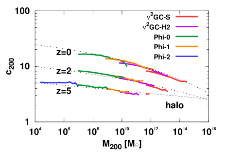
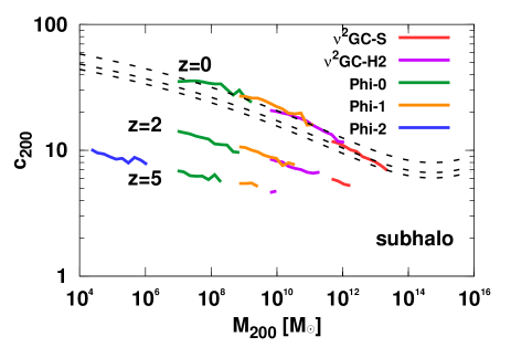
Figure 6: Concentrations $c_{200}$ of field haloes (left) and subhaloes (right) as a function of the halo mass $M_{\rm 200}$. Upper, middle, and lower solid curves are results at $z=0,2$, and 5, respectively. Three thin dashed curves in the left panel are fitting functions proposed by Correa et al. (2015). Three thick dashed curves in the right panel show the model of (Moliné et al., 2017) with $x_{\rm sub}=0.1,0.3$, and 0.5 (upper to bottom), respectively.

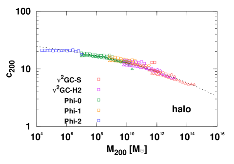
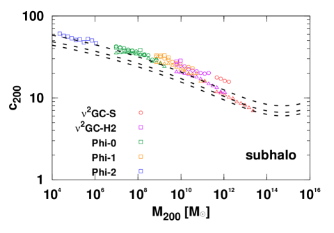
Figure 7: Scaled concentrations of field haloes (left) and subhaloes (right) to $z=0$ as a function of the halo mass $M_{200}$. For field haloes, the concentrations are scaled by multiplying $[H(z)/H(0)]^{2/3}$. For subhaloes, the scaling $(1+z)$ is used. Triangles, circles, and squares show the results at $z=0,2,5$, respectively. Thin dashed curves in the left panel are fitting functions proposed by Correa et al. (2015). Three thick dashed curves in the right panel show the model of Moliné et al. (2017) with $x_{\rm sub}=0.1,0.3$, and 0.5 (upper to bottom), respectively.

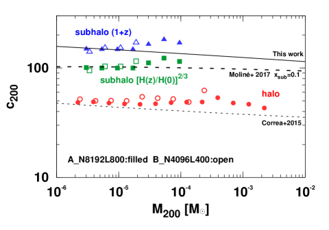
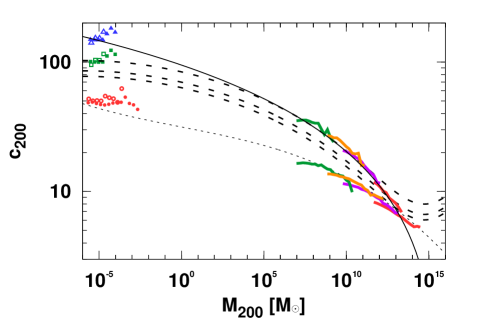
Figure 8: Converted concentrations of the density profiles of haloes and subhaloes near the free streaming scale versus the halo mass. As described in § 3.2, the concentrations are converted to counterparts of the NFW profile at $z=0$. Thin and thick dashed curves are fitting functions proposed by Correa et al. (2015) and Moliné et al. (2017) with $x_{\rm sub}=0.1$, respectively. Solid curve is the fitting function proposed in this work (Equation (5) in the text).

To estimate the contributions of subhaloes near the free streaming scale to gamma-ray annihilation signals, extrapolating the density profiles to $z=0$ is necessary. Under the assumption that the shape parameter is unchanged with the redshift, the commonly used extrapolation of the concentration is the multiplier $(1+z)$ (e.g., Bullock et al., 2001) and $[H(z)/H(0)]^{2/3}$(Macciò et al., 2008; Pilipenko et al., 2017), where $H(z)$ is the Hubble constant. However, the validity of these scaling for subhaloes and less massive field haloes are not fully understood.

We first test the evolution of the concentration of subhaloes and less massive haloes from five cosmological $N$-body simulations as described in Table 2. We selected all haloes and subhaloes that contain more than 1,000 particles. The mass-concentration relation for field haloes has been refined until today (e.g., Prada et al., 2012; Correa et al., 2015; Klypin et al., 2016; Okoli & Afshordi, 2016; Pilipenko et al., 2017; Child et al., 2018; Diemer & Joyce, 2019) and that for less massive field haloes has been studied down to $\sim 10^{7}$$\rm M_{\odot}$ to date (e.g., Pilipenko et al., 2017). It is also studied for near the free streaming scale ($\leq\sim 10^{-3}$$\rm M_{\odot}$, Ishiyama, 2014). However, the relation between $10^{-3}$ and $10^{7}$$\rm M_{\odot}$ is not understood well. Our simulations enable us to test first it down to $\sim 10^{4}$$\rm M_{\odot}$.

We use $M_{\rm 200}$ and $c_{\rm 200}$ instead of $M_{\rm vir}$ and $c_{\rm vir}=r_{\rm vir}/r_{\rm s}$ to compare easily with relevant studies (e.g., Correa et al., 2015; Moliné et al., 2017). Here, $M_{\rm 200}$ is the enclosed mass within $r_{\rm 200}$ in which the spherical overdensity is 200 times the critical density in the Universe. Normally, $c_{\rm 200}$ is defined by $c_{\rm 200}=r_{200}/r_{\rm s}$, however, we calculate it using the maximum circular velocity and the circular velocity at $r_{200}$ with the assumption of the NFW profile, according to the method described in Klypin et al. (2011); Prada et al. (2012); Pilipenko et al. (2017).

Figure 6 shows the mass-concentration relations of field haloes and subhaloes as a function of $M_{\rm 200}$ from $\sim 10^{4}$ to $\sim 10^{15}{\rm M_{\odot}}$ at $z=0,2$ and 5. The fitting functions proposed by Correa et al. (2015) well describe the concentrations of field haloes. On the other hand, concentrations are significantly larger in subhaloes than field haloes, and the slope of mass-concentration relation is steeper in subhaloes. The subhalo concentration at $z=0$ agrees well with the fitting function proposed by Moliné et al. (2017), which also includes the dependence of the distance between the centre of the host halo and the subhalo , $x_{\rm sub}$.

The multiplication $[H(z)/H(0)]^{2/3}$ with the concentrations of field haloes works well, as shown in Figure 7. On the other hand, interestingly, the multiplication $(1+z)$ well matches for subhaloes over the broad mass range. We do not pursue the physical origin of this scaling difference here because it is beyond the scope of this paper. We evaluate the difference between both scaling on the annihilation signal in § 4.

Finally, we convert the mass-concentration relation of haloes and subhaloes near the free streaming scale from $z=32$ to 0. However, our simulations reveal that the density profiles in the cutoff simulation significantly deviate from the NFW profile and have the dependence on the halo mass. Therefore, our results should not be directly comparable with the mass-concentration relation proposed by other studies assuming the universal NFW profile.

To perform an indirect comparison, we converted the concentrations to that of the NFW profile by a method used in other literature (e.g., Ricotti, 2003; Anderhalden & Diemand, 2013; Ishiyama, 2014). The concentration in the profile of Equation (2) can be converted to the equivalent NFW concentration by multiplying $1.0/(2.0-\alpha)$. The extrapolation from $z=32$ to 0 is tested by multiplying $[H(z)/H(0)]^{2/3}$ for haloes and both $[H(z)/H(0)]^{2/3}$ and $(1+z)$ for subhaloes.

Figure 8 plots the converted mass-concentration relation of haloes and subhaloes for the A_N8192L800 and B_N4096L400 simulations against halo mass. The halo concentration shows excellent agreement with Correa et al. (2015), which is calibrated by more massive haloes (galaxy to cluster scale) and lower redshifts, although there is the small systematic upper shift. The redshift scaling of Correa et al. (2015) is slower than both $[H(z)/H(0)]^{2/3}$ and $(1+z)$, explaining this difference to some degree. The halo concentration is slightly smaller those found in earlier simulations (Ishiyama, 2014) because of the usage of the scaling $(1+z)$ in the literature, which gives the higher concentrations than the scaling $[H(z)/H(0)]^{2/3}$.

The subhalo concentration with the scaling $[H(z)/H(0)]^{2/3}$ agrees well with the model of Moliné et al. (2017) using $x_{\rm sub}=0.1$. The subhalo concentration with the scaling $(1+z)$ gives the largest concentration. We suggest a simple fitting function of this subhalo concentration-mass relation for the smallest to the largest resolved scale ($10^{-6}\sim 10^{12}{\rm M_{\odot}}$) as,

$$c_{200}=\sum^{3}_{i=0}c_{i}\times\left[\ln\left(\frac{m_{200}}{\rm M_{\odot}}\right)\right]^{i},$$ (5)

where, $c_{i}=[94.6609,-4.1160,3.3747\times 10^{-2},2.0932\times 10^{-4}]$. This simple functional form is the same used in Lavalle et al. (2008); Sánchez-Conde & Prada (2014). These parameterizations agree well with the subhalo mass-concentration relation as shown in Figure 8 and also match it in more massive subhaloes from $\sim 10^{4}$ to $\sim 10^{12}$$\rm M_{\odot}$.

4 Discussions

In this section, we evaluate the impact of the subhalo mass function and the subhalo density profile obtained in this paper on the annihilation boost factor. All subhaloes contribute the annihilation luminosity of a host halo. The boost factor $B(M)$ is given by (e.g., Strigari et al., 2007; Moliné et al., 2017)

$$B(M) = \frac{3}{L_{\rm host}(M)}\int^{M}_{M_{\rm min}}\frac{dn}{dm}\,dm\int^{1}_{0}\,dx_{\rm sub}\times$$ (6)

$$[1+B_{\rm sub}(m)]\,L_{\rm sub}(m,x_{\rm sub})\,x^{2}_{\rm sub}$$

where, $L_{\rm host}(M)$ and $L_{\rm sub}(M,x_{\rm sub})$ is the annihilation luminosity of a halo and subhalo of mass $M$ with a smooth distribution (without subhaloes), $dn/dm$ is the subhalo mass function, and $x_{\rm sub}=r/r_{200}$. Here, $r$ is the the distance from the centre of the host halo, and we incorporated the dependence of the concentration on $r$ by the way described in (iv) below. We computed the annihilation luminosity of each mass halo by performing numerical integration in volume of the square of Equation (2), from $10^{-5}\rm pc$ to tidal radii of subhaloes (See (v) below).

Based on the results of previous sections, we use the following model to estimate the annihilation boost factor at $z=0$.

1. Density profiles of host haloes: We assume the NFW profile for host haloes and the mass-concentration relation proposed by Correa et al. (2015).

2. Subhalo mass function: As a fiducial model, we use a fitting formula proposed by Ando et al. (2019a), which is based on a successful semianalytic model of subhaloes (Hiroshima et al., 2018). For comparison, we also adopt the subhalo mass function, $dn/dm=0.012M^{-1}(m/M)^{-2.0}$ (e.g. Sánchez-Conde & Prada, 2014; Moliné et al., 2017), which however overpredicts the subhalo abundance (Hiroshima et al., 2018). To incorporate the effect of cutoff, we multiply the subhalo mass functions by the correction functions given by Equation (1). We use $M_{1}=1.3\times 10^{-6}$ and $M_{2}=1.0\times 10^{-7}$ (correction function 2) by default. however we also test $M_{2}=1.0\times 10^{-8}$ (correction function 1). The smallest limit of the integral (6) is $M_{\rm min}=10^{-6}$$\rm M_{\odot}$.

3. Density profiles of subhaloes: The slope $\alpha$ in subhalo density profiles are described by Equation (4). When they give values smaller than one, $\alpha$ is forced to be one under the assumption that the profile is like the NFW profile. Although $\alpha$ is less than one for the most massive two bins as seen in Figure 4, we force to be one to smoothly connect to the profile of more massive subhalos, which is reasonably well fitted by the NFW profile (Springel et al., 2008).

4. The mass-concentration relation of subhaloes: If $\alpha>1$, the concentration is converted to that of the double power law function employing the opposite way described in §3.3. Extrapolation to z=0 is done by multiplying $(1+z)$. We assume the average concentration as a function of subhalo mass is described by Equation (5), and modify it to incorporate the dependence of the concentration on the distance from the centre of the host halo $r$, as $0.95c_{200}(m_{200})[1.0-0.54\log_{10}(x_{\rm sub})]$, where $c_{200}(m_{200})$ is the same with Equation (5) and $x_{\rm sub}=r/r_{200}$. Dependence on the distance is following Moliné et al. (2017), and the normalization is determined with the assumption that $0.81r_{200}$ is the average position of subhaloes (Springel et al., 2008). As described in §3.3, the extrapolation of the mass-concentration relation has considerable uncertainty. Thus, we also compute the boost factor using the fitting function proposed by Moliné et al. (2017), which gives quantitatively good agreement with our simulation results when the scaling $[H(z)/H(0)]^{2/3}$ is used. We integrated $x_{\rm sub}$ from the centre to 1 ($r=r_{200}$) of the host halo assuming subhaloes distribute uniformly. We call the former “high concentration” and the latter “low concentration” model.

5. Tidal radius: We calculate the tidal radii of subhaloes by following Moliné et al. (2017).

Figure 9 shows the annihilation boost factor versus the host halo mass. For the fiducial subhalo mass function (Ando et al., 2019a), the boost factors of a Milky-Way sized halo ($M\sim 2.0\times 10^{12}M_{\odot}$) are $\sim 6.23$ and $1.75$ for models of “high” and “low concentration”, respectively. Those with another subhalo mass function are $\sim 118$ and $27$, respectively. In the latter case, our models raise the boost factor substantially, by a factor of four compared with that using the mass-concentration relation of field haloes, which gives the boost factors $\sim 29$ (Ishiyama, 2014). However, such considerable boost might be unrealistic because the fiducial subhalo mass function is favoured (Hiroshima et al., 2018; Ando et al., 2019a).

When we apply the other correction function for the subhalo mass function (correction function 1), the resulting boost factor of a Milky-Way sized halo is nearly the same with the other correction function. Without the correction function of the subhalo mass function, the boost factor of a Milky-Way sized halo becomes 6.65 for the “high concentration” model. On the other hand, when we force the NFW profile for all subhaloes, the resulting boost factor is 5.96. Thus, the suppression of the subhalo abundance near the free streaming scale reduces the boost by $\sim 6\%$ and the steeper cusp increase it by $\sim 5\%$, indicating that both effects compensate each other. This explains the reason that the boost factors of our model and Moliné et al. (2017) agree well with each other when the same subhalo mass function and the mass-concentration relation for subhaloes are used. The deviation at high mass end reflects the difference of adopted mass-concentration relation for host haloes. The relation of Sánchez-Conde & Prada (2014) adopted in Moliné et al. (2017) gives higher concentrations at high mass end than that of Correa et al. (2015) adopted in this work. Thus, resulting boost factors are smaller in Moliné et al. (2017).

There is a good agreement between the model of high concentration with the fiducial subhalo mass function and the model of Moliné et al. (2017) with $dn/dm=0.03M^{-1}(m/M)^{-1.9}$. The latter subhalo mass function gives a larger number of subhalos than the fiducial one, not so much as that with the slope $-2$. This is a reason that both boost factors agree well, whereas the concentration in the former is substantially high.

In these calculations, we ignore the contribution of subhaloes below $10^{-6}M_{\odot}$. The density profile of haloes and subhaloes below the cutoff scale is not understood well, and the assumption for it in our model might be invalid. We will address this subject in a future paper. However, our results suggest that the existence of the cutoff on the subhalo mass function could obscure this uncertainty and allow us to estimate the annihilation signal robustly if the mass-concentration relation is given correctly.

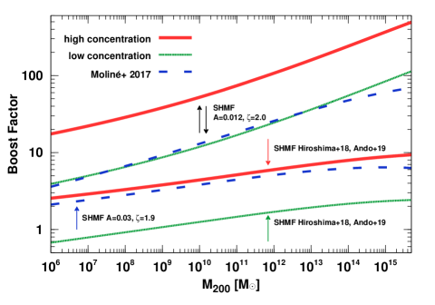
Figure 9: Annihilation boost factor as a function of the host halo mass. Two different mass-concentration relations for subhaloes are used. Upper solid and dotted curves are our model results with the subhalo mass function (SHMF) $dn/dm=AM^{-1}(m/M)^{-\zeta}$ ($A=0.012$ and $\zeta=2.0$). Bottom solid and dotted curves are results with the subhalo mass function proposed by Ando et al. (2019a), which is based on a successful semianalytic model of subhaloes (Hiroshima et al., 2018). Dashed curves are from Moliné et al. (2017) with two different subhalo mass functions. Upper and lower ones use $A=0.012,\zeta=2.0$ and $A=0.03,\zeta=1.9$, respectively.

5 Summary

We have studied the abundance and structure of subhaloes near the free streaming scale using a suite of unprecedentedly large cosmological $N$-body simulations. We used two different models of initial matter power spectra with and without the cutoff, which is resulted from the free streaming damping of WIMP dark matter particle. We have investigated the effect of cutoff on the subhalo mass function and the density profile of subhalo. Our primary results are summarized below.

1. For the range of host halo mass between $10^{-4}$ and $10^{-2}$$\rm M_{\odot}$, the subhalo mass functions in the cutoff simulation agree with those in the no cutoff simulation for masses more massive than $\sim 5.0\times 10^{-6}$$\rm M_{\odot}$. For the less massive subhaloes, the slopes of mass functions $\zeta$ are gradually decreasing with decreasing subhalo mass differently from the no cutoff simulation, and are becoming flat at around $\sim 10^{-6}$$\rm M_{\odot}$, which corresponds to the cutoff scale. The slopes $\zeta$ are becoming steeper again from $\sim 10^{-7}$$\rm M_{\odot}$ due to artificial fragmentation as seen in warm dark matter simulations. The ratio between the subhalo mass function in the cutoff and no cutoff simulation is well fitted by the correction function described in Equation (1), regardless of the host halo mass and the redshift.

2. In subhaloes, the central slopes are considerably shallower than in field haloes for both simulations with and without the cutoff, but are still steeper than that of the NFW profile. The shape parameter $\alpha$ is given by $-0.296\log_{10}(M_{\rm vir}/10^{-6}{\rm M_{\odot}})+1.473$.

3. The concentrations are significantly larger in subhaloes than haloes and depend on the subhalo mass because of the tidal stripping. This picture is qualitatively consistent with what we see in more massive haloes (e.g., Ghigna et al., 2000; Bullock et al., 2001; Moliné et al., 2017).

4. We compare two methods to extrapolate the mass-concentration relation of haloes and subhaloes to z=0 and provide a new simple fitting function for subhaloes, based on a suite of large cosmological $N$-body simulations. Finally, we estimate the annihilation boost factor of a Milky-Way sized halo to be between 1.8 and 6.2.

References

- Anderhalden & Diemand (2013) Anderhalden D., Diemand J., 2013, J. Cosmology Astropart. Phys., 4, 9
- Anderson et al. (2016) Anderson B., Zimmer S., Conrad J., Gustafsson M., Sánchez-Conde M., Caputo R., 2016, J. Cosmology Astropart. Phys., 2, 026
- Ando et al. (2008) Ando S., Kamionkowski M., Lee S. K., Koushiappas S. M., 2008, Phys. Rev. D, 78, 101301
- Ando et al. (2019a) Ando S., Ishiyama T., Hiroshima N., 2019a, Galaxies, 7, 68
- Ando et al. (2019b) Ando S., Kamada A., Sekiguchi T., Takahashi T., 2019b, Phys. Rev. D, 100, 123519
- Angulo et al. (2013) Angulo R. E., Hahn O., Abel T., 2013, MNRAS, 434, 3337
- Angulo et al. (2017) Angulo R. E., Hahn O., Ludlow A. D., Bonoli S., 2017, MNRAS, 471, 4687
- Baghram et al. (2011) Baghram S., Afshordi N., Zurek K. M., 2011, Phys. Rev. D, 84, 043511
- Bartels & Ando (2015) Bartels R., Ando S., 2015, Phys. Rev. D, 92, 123508
- Behroozi et al. (2013) Behroozi P. S., Wechsler R. H., Wu H.-Y., 2013, ApJ, 762, 109
- Berezinsky et al. (2003) Berezinsky V., Dokuchaev V., Eroshenko Y., 2003, Phys. Rev. D, 68, 103003
- Berezinsky et al. (2008) Berezinsky V., Dokuchaev V., Eroshenko Y., 2008, Phys. Rev. D, 77, 083519
- Bertschinger (2006) Bertschinger E., 2006, Phys. Rev. D, 74, 063509
- Bird et al. (2016) Bird S., Cholis I., Muñoz J. B., Ali-Haïmoud Y., Kamionkowski M., Kovetz E. D., Raccanelli A., Riess A. G., 2016, Physical Review Letters, 116, 201301
- Bryan & Norman (1998) Bryan G. L., Norman M. L., 1998, ApJ, 495, 80
- Bullock et al. (2001) Bullock J. S., Kolatt T. S., Sigad Y., Somerville R. S., Kravtsov A. V., Klypin A. A., Primack J. R., Dekel A., 2001, MNRAS, 321, 559
- Chen & Koushiappas (2010) Chen J., Koushiappas S. M., 2010, ApJ, 724, 400
- Child et al. (2018) Child H. L., Habib S., Heitmann K., Frontiere N., Finkel H., Pope A., Morozov V., 2018, ApJ, 859, 55
- Correa et al. (2015) Correa C. A., Wyithe J. S. B., Schaye J., Duffy A. R., 2015, MNRAS, 452, 1217
- Crocce et al. (2006) Crocce M., Pueblas S., Scoccimarro R., 2006, MNRAS, 373, 369
- Delos (2019) Delos M. S., 2019, Phys. Rev. D, 100, 063505
- Delos et al. (2018a) Delos M. S., Erickcek A. L., Bailey A. P., Alvarez M. A., 2018a, Phys. Rev. D, 97, 041303
- Delos et al. (2018b) Delos M. S., Erickcek A. L., Bailey A. P., Alvarez M. A., 2018b, Phys. Rev. D, 98, 063527
- Delos et al. (2019) Delos M. S., Bruff M., Erickcek A. L., 2019, Phys. Rev. D, 100, 023523
- Diamanti et al. (2015) Diamanti R., Catalan M. E. C., Ando S., 2015, Phys. Rev. D, 92, 065029
- Diemand et al. (2005) Diemand J., Moore B., Stadel J., 2005, Nature, 433, 389
- Diemand et al. (2007) Diemand J., Kuhlen M., Madau P., 2007, ApJ, 657, 262
- Diemer & Joyce (2019) Diemer B., Joyce M., 2019, ApJ, 871, 168
- Erickcek (2015) Erickcek A. L., 2015, Phys. Rev. D, 92, 103505
- Erickcek & Law (2011) Erickcek A. L., Law N. M., 2011, ApJ, 729, 49
- Fornasa & Sánchez-Conde (2015) Fornasa M., Sánchez-Conde M. A., 2015, Phys. Rep., 598, 1
- Ghigna et al. (2000) Ghigna S., Moore B., Governato F., Lake G., Quinn T., Stadel J., 2000, ApJ, 544, 616
- Goerdt et al. (2007) Goerdt T., Gnedin O. Y., Moore B., Diemand J., Stadel J., 2007, MNRAS, 375, 191
- González-Morales et al. (2013) González-Morales A. X., Valenzuela O., Aguilar L. A., 2013, J. Cosmology Astropart. Phys., 3, 001
- Gosenca et al. (2017) Gosenca M., Adamek J., Byrnes C. T., Hotchkiss S., 2017, Phys. Rev. D, 96, 123519
- Green et al. (2004) Green A. M., Hofmann S., Schwarz D. J., 2004, MNRAS, 353, L23
- Hahn & Abel (2011) Hahn O., Abel T., 2011, MNRAS, 415, 2101
- Hiroshima et al. (2018) Hiroshima N., Ando S., Ishiyama T., 2018, Phys. Rev. D, 97, 123002
- Hofmann et al. (2001) Hofmann S., Schwarz D. J., Stöcker H., 2001, Phys. Rev. D, 64, 083507
- Hooper & Witte (2017) Hooper D., Witte S. J., 2017, J. Cosmology Astropart. Phys., 4, 018
- Hütten et al. (2016) Hütten M., Combet C., Maier G., Maurin D., 2016, J. Cosmology Astropart. Phys., 9, 047
- Hütten et al. (2018) Hütten M., Combet C., Maurin D., 2018, J. Cosmology Astropart. Phys., 2, 005
- Ishiyama (2014) Ishiyama T., 2014, ApJ, 788, 27
- Ishiyama et al. (2009) Ishiyama T., Fukushige T., Makino J., 2009, PASJ, 61, 1319
- Ishiyama et al. (2010) Ishiyama T., Makino J., Ebisuzaki T., 2010, ApJ, 723, L195
- Ishiyama et al. (2012) Ishiyama T., Nitadori K., Makino J., 2012, in Proc. Int. Conf. High Performance Computing, Networking, Storage and Analysis, SC’12 (Los Alamitos, CA: IEEE Computer Society Press), 5:, (arXiv:1211.4406). http://dl.acm.org/citation.cfm?id=2388996.2389003
- Ishiyama et al. (2015) Ishiyama T., Enoki M., Kobayashi M. A. R., Makiya R., Nagashima M., Oogi T., 2015, PASJ, 67, 61
- Ishiyama et al. (2016) Ishiyama T., Sudo K., Yokoi S., Hasegawa K., Tominaga N., Susa H., 2016, ApJ, 826, 9
- Karwin et al. (2019) Karwin C. M., Murgia S., Campbell S., Moskalenko I. V., 2019, ApJ, 880, 95
- Kashiyama & Oguri (2018) Kashiyama K., Oguri M., 2018, preprint, (arXiv:1801.07847)
- Klypin et al. (2011) Klypin A. A., Trujillo-Gomez S., Primack J., 2011, ApJ, 740, 102
- Klypin et al. (2016) Klypin A., Yepes G., Gottlöber S., Prada F., Heß S., 2016, MNRAS, 457, 4340
- Koushiappas (2006) Koushiappas S. M., 2006, Physical Review Letters, 97, 191301
- Koushiappas et al. (2004) Koushiappas S. M., Zentner A. R., Walker T. P., 2004, Phys. Rev. D, 69, 043501
- Lacey & Cole (1994) Lacey C., Cole S., 1994, MNRAS, 271, 676
- Lavalle et al. (2008) Lavalle J., Yuan Q., Maurin D., Bi X.-J., 2008, A&A, 479, 427
- Loeb & Zaldarriaga (2005) Loeb A., Zaldarriaga M., 2005, Phys. Rev. D, 71, 103520
- Macciò et al. (2008) Macciò A. V., Dutton A. A., van den Bosch F. C., 2008, MNRAS, 391, 1940
- Makiya et al. (2016) Makiya R., et al., 2016, PASJ, 68, 25
- Marchegiani & Colafrancesco (2016) Marchegiani P., Colafrancesco S., 2016, J. Cosmology Astropart. Phys., 11, 033
- Moliné et al. (2017) Moliné Á., Sánchez-Conde M. A., Palomares-Ruiz S., Prada F., 2017, MNRAS, 466, 4974
- Navarro et al. (1997) Navarro J. F., Frenk C. S., White S. D. M., 1997, ApJ, 490, 493
- Nitadori et al. (2006) Nitadori K., Makino J., Hut P., 2006, New Astron., 12, 169
- Ogiya & Hahn (2018) Ogiya G., Hahn O., 2018, MNRAS, 473, 4339
- Ogiya et al. (2016) Ogiya G., Nagai D., Ishiyama T., 2016, MNRAS, 461, 3385
- Okoli & Afshordi (2016) Okoli C., Afshordi N., 2016, MNRAS, 456, 3068
- Peñarrubia (2018) Peñarrubia J., 2018, MNRAS, 474, 1482
- Pilipenko et al. (2017) Pilipenko S. V., Sánchez-Conde M. A., Prada F., Yepes G., 2017, MNRAS, 472, 4918
- Planck Collaboration et al. (2014) Planck Collaboration et al., 2014, A&A, 571, A16
- Planck Collaboration et al. (2016) Planck Collaboration et al., 2016, A&A, 594, A13
- Planck Collaboration et al. (2018) Planck Collaboration et al., 2018, preprint, (arXiv:1807.06209)
- Polisensky & Ricotti (2015) Polisensky E., Ricotti M., 2015, MNRAS, 450, 2172
- Prada et al. (2012) Prada F., Klypin A. A., Cuesta A. J., Betancort-Rijo J. E., Primack J., 2012, MNRAS, 423, 3018
- Profumo et al. (2006) Profumo S., Sigurdson K., Kamionkowski M., 2006, Physical Review Letters, 97, 031301
- Ricotti (2003) Ricotti M., 2003, MNRAS, 344, 1237
- Sánchez-Conde & Prada (2014) Sánchez-Conde M. A., Prada F., 2014, MNRAS, 442, 2271
- Schneider et al. (2013) Schneider A., Smith R. E., Reed D., 2013, MNRAS, 433, 1573
- Springel et al. (2008) Springel V., et al., 2008, MNRAS, 391, 1685
- Stref & Lavalle (2017) Stref M., Lavalle J., 2017, Phys. Rev. D, 95, 063003
- Strigari et al. (2007) Strigari L. E., Koushiappas S. M., Bullock J. S., Kaplinghat M., 2007, Phys. Rev. D, 75, 083526
- Tanikawa et al. (2012) Tanikawa A., Yoshikawa K., Okamoto T., Nitadori K., 2012, New Astron., 17, 82
- Tanikawa et al. (2013) Tanikawa A., Yoshikawa K., Nitadori K., Okamoto T., 2013, New Astron., 19, 74
- Van Tilburg et al. (2018) Van Tilburg K., Taki A.-M., Weiner N., 2018, J. Cosmology Astropart. Phys., 2018, 041
- Wang & White (2007) Wang J., White S. D. M., 2007, MNRAS, 380, 93
- Yoshikawa & Tanikawa (2018) Yoshikawa K., Tanikawa A., 2018, Research Notes of the American Astronomical Society, 2, 231
- Zybin et al. (1999) Zybin K. P., Vysotsky M. I., Gurevich A. V., 1999, Physics Letters A, 260, 262