Observational Constraints on Warm Inflation in Loop Quantum Cosmology

Abstract

By incorporating quantum aspects of gravity, Loop Quantum Cosmology (LQC) provides a self-consistent extension of the inflationary scenario, allowing for modifications in the primordial inflationary power spectrum with respect to the standard General Relativity one. We investigate such modifications and explore the constraints imposed by the Cosmic Microwave Background (CMB) Planck Collaboration data on the Warm Inflation (WI) scenario in the LQC context. We obtain useful relations between the dissipative parameter of WI and the bounce scale parameter of LQC. We also find that the number of required e-folds of expansion from the bounce instant till the moment the observable scales crossed the Hubble radius during inflation can be smaller in WI than in CI. In particular, we find that this depends on how large is the dissipation in WI, with the amount of required e-folds decreasing with the increasing of the dissipation value. Furthermore, by performing a Monte Carlo Markov Chain analysis for the considered WI models, we find good agreement of the model with the data. This shows that the WI models studied here can explain the current observations also in the context of LQC.

1 Introduction

In the last years we have witnessed the release of a large amount of precision data, from the Cosmic Microwave Background (CMB) [1, 2] to large scale structures [3, 4, 5], including Barionic Acoustic Oscillation data [6, 7], both strong and weak lensing [8, 9, 10], galaxy cluster number counts [11, 12] and so on, up to gravitational waves detections [13, 14, 15]. This has allowed us to obtain valuable information about the nature and the evolution of the universe, as well as the mechanisms operating at the very early times (see, e.g., refs. [16] and [17]). The current paradigm for the cosmology of the early universe is inflation, which besides of solving the problems of the standard Big Bang cosmology, provides a causal explanation for the origin of the CMB anisotropies and the large-scale structure of the universe [18] (see also ref. [19]). The inflationary scenario was developed long before accurate data were available, which makes it a very predictive scenario. However, the recent CMB data imposed a big challenge for some classes of inflationary models by putting severe constrains on many of them [20].

The description of inflation can be classified in two scenarios according to the dynamics of the inflaton field. In the Cold Inflation (CI) scenario, interactions of the inflaton with other field degrees of freedom are not enough to counter balance the dilution of any possible pre-existing or newly formed radiation and the universe super freezes. Density perturbations are originated as quantum fluctuations of the inflaton field [21]. In the Warm Inflation (WI) scenario [22] (see also refs. [23, 24] for reviews), on the other hand, the interactions of the inflaton with other field degrees of freedom (and also among the latter) can be sufficient to produce a quasi-stationary thermalized radiation bath throughout inflation. The primary source of density fluctuations in this case can come entirely from thermal fluctuations originated in the radiation bath and transported to the inflaton field as adiabatic curvature perturbations [25, 26, 27, 28, 29]. In the WI picture, the presence of nontrivial dynamics, accounting for dissipative and stochastic effects, cause a significant impact on the usual observational quantities like in the tensor-to-scalar ratio, $r$, the spectral index, $n_{s}$, and the non-Gaussianity parameter, $f_{NL}$ [30, 31, 32, 33, 34, 35]. Due to these modifications, some classes of inflaton potentials excluded in the CI context by the data can be rehabilitated in the WI context, as it is the case of the monomial chaotic potentials for instance. In the WI scenario the coupling between the inflaton and other fields might be strong enough to lead to a significant radiation production rate, while still preserving the expected flatness of the inflaton potential. The radiation production during WI can compensate for the supercooling of the universe observed in CI, thus making possible for a smooth transition from the inflationary accelerated expansion to the radiation dominate phase, without the need or a presence of a (pre)reheating phase following the end of the inflationary regime.

One important aspect to point out is that the WI scenario, as is also true for the CI one, they are both sensitive to the ultraviolet (UV) physics, and their successes are tightly dependent on the understanding of such UV physics in general. Inflationary space-times inherit the big-bang singularity. Physically, this occurs because one continues to use General Relativity (GR) theory even in the Planck regime where it is supposed not to be applicable. It is widely expected that new physics in this regime will resolve the singularity, significantly changing the very early history of the universe. One of the possible scenarios that takes into account a new physics in this high energy regime is Loop Quantum Gravity (LQG), which is believed to be a possible candidate for a quantum theory of gravity (see, e.g., refs. [36, 37, 38, 39, 40] for some recent reviews). Loop Quantum Cosmology (LQC) arises as the result of applying principles of LQG to cosmological settings (see, e.g., refs. [38, 39, 40] for recent reviews). In LQC the quantum geometry creates a brand new repulsive force, which is totally negligible at low space-time curvature but rises very rapidly in the Planck regime, overwhelming the classical gravitational attraction. In cosmological models, Einstein’s equations undergo modifications in the Planck regime. For matter satisfying the usual energy conditions, any time a curvature invariant grows to the Planck scale, quantum geometry effects dilute it, resolving singularities of the GR [41, 42, 43]. These quantum gravitational effects are expected to dominate the Planck era of the universe causing a quantum bounce to appear and that replaces the classical big bang singularity. Usually, in these scenarios, where inflation is studied in the context of LQC, the inflaton potential is assumed to be simply a quadratic potential for the inflaton field. Very close to the bounce quantum gravity effects dominate the dynamics, but these effects lessen shortly after such that the potential $V(\phi)$ begins to prevail, starting the inflationary phase. Though this picture is the most common in the literature and the one we will adopt also here, there are also other possibilities, with the dominant field at the bounce depending on the cosmological scenario being considered. Also, in the context of inflation it is not necessary to only consider scalar fields with a quadratic potential, with other potentials being equally possible. In this work, we will consider in fact a quartic monomial chaotic potential for the inflaton. Therefore, LQC provides an interesting arena to incorporate the highest energy density and curvature stages of the universe into cosmological models, where questions about Planck-scale physics and initial conditions for inflation can be addressed [44].

Cosmological perturbations are generally described by quantum fields on classical, curved space-times. However this strategy cannot be trivially justified in the quantum gravity era, when curvature and matter densities are of Planck scale. Nevertheless, using techniques from LQG, the standard theory of cosmological perturbations was extended to overcome this limitation [45]. The dressed metric approach [46, 47, 48, 45] is able to provide this extension, while having the advantage of allowing ones to describe the main perturbation equations in a form analogous to the classical one [45, 48]. Also, the pre-inflationary evolution makes scalar and tensor perturbations reach the onset of inflation in an excited state [47], so that the primordial spectra that source the CMB anisotropies acquire extra features with quantum gravitational origin from the pre-inflationary era.

Previous studies on both CI and WI in the context of LQC showed interesting features regarding properties of the pre-inflationary phase and the start of inflation itself [58, 49, 50, 51, 52, 53, 54, 55, 56, 57]. In the present work we focus for the first time on the problem of confronting the observational predictions of WI in LQC with the latest CMB data. By accounting for the modifications of the spectrum of primordial perturbations resulted from the LQC, we compute the number of extra e-folds required in this model for it to be compatible with the observations and put constraints on the LQC parameters when in the WI context. Finally, we focus on analyzing the relation of these characteristic parameters of LQC with the dissipative parameter of WI.

This paper is organized as follows. In section 2 we describe the theoretical context of the WI scenario in LQC, deriving the equations we use in our analysis. The method and observational dataset are discussed in section 3, where we also present and discuss our results. Finally, in section 4 we summarize our conclusions.

2 Theoretical context

In this section we briefly review some of the most relevant aspects of LQC and WI, then showing the expressions for their observables in the WI scenario in LQC, which will be considered in our analysis in the next section.

2.1 Loop Quantum Cosmology dynamics

The spatial geometry in LQC is encoded in the volume of a fixed fiducial cubic cell, rather than the scale factor $a$, and is given by

$$v=\frac{4{\cal V}_{0}a^{3}M_{\rm Pl}^{2}}{\gamma},$$ (2.1)

where ${\cal V}_{0}$ is the comoving volume of the fiducial cell, $\gamma$ is the Barbero-Immirzi parameter of LQC, whose numerical value we set as given by $\gamma\simeq 0.2375$ [59], and $M_{\rm Pl}\equiv 1/\sqrt{8\pi G}=2.4\times 10^{18}$GeV is the reduced Planck mass. The conjugate momentum to $v$ is denoted by $b$ and it is given by $b=-\gamma P_{(a)}/(6a^{2}{\cal V}_{0}M_{\rm Pl}^{2})$, where $P_{(a)}$ is the conjugate momentum to the scale factor.

The solution of the LQC effective equations implies that the Hubble parameter, $H$, can be written as

$$H=\frac{1}{2\gamma\lambda}\sin(2\lambda b).$$ (2.2)

where $\lambda=\sqrt{\sqrt{3}\gamma/(2M_{\rm Pl}^{2})}$ and $b$ ranges over $(0,\pi/\lambda)$. The energy density, $\rho$, relates to the LQC variable $b$ through $\rho=3M_{\rm Pl}^{2}\sin^{2}(\lambda b)/(\gamma^{2}\lambda^{2})$. Then, the Friedmann’s equation in LQC assumes the form [60],

$$\frac{1}{9}\left(\frac{\dot{v}}{v}\right)^{2}\equiv H^{2}=\frac{1}{3M_{\rm Pl}^{2}}\rho\left(1-\frac{\rho}{\rho_{\rm cr}}\right),$$ (2.3)

where $\rho_{\rm cr}=3M_{\rm Pl}^{2}/(\gamma^{2}\lambda^{2})$. For $\rho\ll\rho_{\rm cr}$ we recover GR as expected. The above expression holds independently of the particular characteristics of the inflationary regime. We can see from eq. (2.3) that the singularity is replaced by a quantum bounce for $H=0$, when the density reaches the critical value $\rho_{\rm cr}$.

In addition to the modifications at the background level from LQC, at the perturbative level some of the relevant modes have physical wavelengths comparable to the curvature radius at the bounce time. Unlike what happens in the CI scenarios in GR, where it is usually assumed that the pre-inflationary dynamics does not have any effect on modes observable in the CMB, in LQC the situation is different. Using techniques from LQG, the standard theory of cosmological perturbations can be extended to encompass the quantum gravity regime, allowing to describe the main perturbation equations in a form analogous to the classical one [45]. Also, modes that experience curvature are excited [61], i.e., large wavelength modes are excited in the Planck regime that follows the bounce. The main effect at the onset of inflation is that the quantum state of perturbations is populated by excitations of these modes over the Bunch-Davis vacuum, changing the initial conditions for perturbations at the onset of inflation [47]. As a consequence, the scalar curvature power spectrum in LQC gets modified with respect to GR, such that it can be written as (see, e.g., ref. [58] for more details and for a complete derivation)

$$\Delta_{\mathcal{R}}(k)=|\alpha_{k}+\beta_{k}|^{2}\Delta_{\mathcal{R}}^{GR}(k).$$ (2.4)

with $\alpha_{k}$ and $\beta_{k}$ are the Bogoliubov coefficients (where the pre-inflationary effects are codified) and $\Delta_{\mathcal{R}}^{GR}$ is the GR form for the power spectrum. It should be noticed that in the Bunch-Davis vacuum, as in the general relativity case, we have that the Bogoliubov coefficients in eq. (2.4) should reduce simply to [61]

$$\alpha_{k}\to\alpha_{k}^{\rm BD}=1,\;\;\;\beta_{k}\to\beta_{k}^{\rm BD}=0,$$ (2.5)

which can be seen as no excited (or produced) particles in the vacuum. In LQC, the change of the spectrum can be seen exactly as a result of the change of the vacuum state with respected to the GR case. This change in the vacuum state can be interpreted as a consequence of gravitational particle production due to the bounce. This becomes even clearer when writing the term $|\alpha_{k}+\beta_{k}|^{2}$ in eq. (2.4) as

$$|\alpha_{k}+\beta_{k}|^{2}=1+2|\beta_{k}|^{2}+2{\rm Re}(\alpha_{k}\beta_{k}^{*}),$$ (2.6)

where $|\beta_{k}|^{2}\equiv n_{k}$ is associated with the number of excitations in the mode $k$ [47]. By following the same notation used by the authors of ref. [58], the above eq. (2.4) is parameterized as

$$\Delta_{\mathcal{R}}(k)=(1+\delta_{PL})\Delta_{\mathcal{R}}^{GR}(k).$$ (2.7)

where the factor $\delta_{PL}$ is scale ($k$-)dependent and takes into account the LQC corrections. It is explicitly given by [58]

$$\delta_{PL} = \left[1+\cos\left(\frac{\pi}{\sqrt{3}}\right)\right]{\rm csch}^{2}\left(\frac{\pi k}{\sqrt{6}k_{B}}\right)$$ (2.8)

$$+ \sqrt{2}\sqrt{\cosh\left(\frac{2\pi k}{\sqrt{6}k_{B}}\right)+\cos\left(\frac{\pi}{\sqrt{3}}\right)}\cos\left(\frac{\pi}{2\sqrt{3}}\right)$$

$$\times {\rm csch}^{2}\left(\frac{\pi k}{\sqrt{6}k_{B}}\right)\cos(2k\eta_{B}+\varphi_{k}),$$

where

$$\varphi_{k}\equiv\arctan\left\{\frac{{\rm Im}[\Gamma(a_{1})\Gamma(a_{2})\Gamma^{2}(a_{3}-a_{1}-a_{2})]}{{\rm Re}[\Gamma(a_{1})\Gamma(a_{2})\Gamma^{2}(a_{3}-a_{1}-a_{2})]}\right\},$$ (2.9)

with $a_{1},\,a_{2},\,a_{3}$ defined as $a_{1,2}=(1\pm 1/\sqrt{3})/2-ik/(\sqrt{6}k_{B})$ and $a_{3}=1-ik/(\sqrt{6}k_{B})$ and the index $B$ in the quantities indicates that they are calculated at the bounce. In particular, $\eta_{B}$ is the conformal time at the bounce and $k_{B}=\sqrt{\rho_{c}}a_{B}/M_{\rm Pl}$ is a characteristic scale also at the bounce, which is the shortest scale (or largest wave number $k$) that feels the space-time curvature during the bounce. We should mention that the expression (2.7) is valid also in the presence of a small amount of radiation during the bounce (which dillutes very fast) in addition to the dominant contribution from the inflaton’s energy density. Comparing eq. (2.8) with eq. (2.6) we identify

$$2|\beta_{k}|^{2} = \left[1+\cos\left(\frac{\pi}{\sqrt{3}}\right)\right]{\rm csch}^{2}\left(\frac{\pi k}{\sqrt{6}k_{B}}\right),$$ (2.10)

$$2{\rm Re}(\alpha_{k}\beta_{k}^{*}) = \sqrt{2}\sqrt{\cosh\left(\frac{2\pi k}{\sqrt{6}k_{B}}\right)+\cos\left(\frac{\pi}{\sqrt{3}}\right)}\cos\left(\frac{\pi}{2\sqrt{3}}\right)$$ (2.11)

$$\times {\rm csch}^{2}\left(\frac{\pi k}{\sqrt{6}k_{B}}\right)\cos(2k\eta_{B}+\varphi_{k}).$$

The term $\cos(2k\eta_{B}+\varphi_{k})$ in eq. (2.11) oscillates very fast, so it has negligible effect when averaging out in time. Then, for any practical purpose, in observable quantities the factor $\delta_{PL}$ can be simply considered as being given by

$$\delta_{PL}=\left[1+\cos\left(\frac{\pi}{\sqrt{3}}\right)\right]{\rm csch}^{2}\left(\frac{\pi k}{\sqrt{6}k_{B}}\right).$$ (2.12)

Note that in this case $\delta_{PL}$ can simply be identified with $2n_{k}$, i.e., with the own number of excitations in the mode $k$ which appears as a consequence of the quantum bounce in LQC. Since this pre-factor represents the effects of the pre-inflationary dynamics, it will appear similarly also in the power spectrum of WI models. The difference, as we will see in the next section, is that in WI there are also the effect of explicitly particle production due to the microscopic processes generating the radiation bath. As a consequence, the factor $2n_{k}$ changing the spectrum due to the departure from the Bunch-Davis vacuum will have two contributions: one, considered in the equations above, due to the LQC bounce effect (hereafter $2n_{k}^{\rm LQC}$) which is given by eq. (2.12), and another due to the particle production inherent of the WI dynamics which we are going to denote by $2n_{k}^{\rm WI}$ (see. e.g., ref. [34] for an explicit derivation of the later).

The same way that the quantum bounce changes the scalar power spectrum like eq. (2.7), likewise the tensor spectrum in the LQC is modified as [58]

$$\Delta_{T}(k)=(1+\delta_{PL})\Delta_{T}^{GR}(k),$$ (2.13)

where $\Delta_{T}^{GR}(k)$ is the tensor spectrum in GR. Again, the term in front of the GR result in eq. (2.13) can be exactly associated with the change of the Bunch-Davis vacuum due to the production of excitations with mode $k$ out of the vacuum and $1+\delta_{PL}\equiv 1+2n_{k}^{\rm LQC}$.

In the following we will denote the number of e-folds for the relevant scales at Hubble crossing as $N_{*}\equiv ln(a_{\rm end}/a_{*})\approx 60$, where $a_{\rm end}$ is the scale factor at the end of inflation and all quantities with subscript $*$ are evaluated when the mode crosses the horizon at $k_{*}=a_{*}H_{*}$. In LQC, in addition to the usual number of e-folds at Hubble crossing $N_{*}$, it is necessary an extra amount of e-folds, $\delta N$, in order for the predictions from the model to be consistent with observations [58]. This is so because, as seen from eq. (2.7), after the effects of the pre-inflationary dynamics from LQC are taken into account, the power spectra are generically scale-dependent through the correction $\delta_{PL}$, eq. (2.12), and also exhibits oscillatory features. As a consequence, in CI in order to be consistent with observations, the universe must have expanded at least [58] around $21$ e-folds from the bounce till Hubble radius crossing of the observables scales, such as to allow for these scale-dependent features to get sufficiently diluted away and not spoiling the perturbation spectra of CMB (see also ref. [63] and references therein for a discussion about these and other LQC effects).

The total number of e-folds of expansion from the moment of the bounce till today, $N_{\rm tot}$, is related to the LQC parameter $k_{B}$ through the equation [58],

$$\frac{k_{B}}{a_{0}}=\sqrt{\frac{\gamma_{B}}{3}}\frac{a_{B}}{a_{0}}m_{pl}=\sqrt{\frac{\gamma_{B}}{3}}m_{pl}e^{N_{\rm tot}}.$$ (2.14)

We note that, by assuming an upper bound on $k_{B}$ as set by eq. (2.14), it can be translated into constraints on the total number of e-folds. This, in turn, leads to a lower bound on the extra number of e-folds of inflation required in LQC, since $\delta N>N_{\rm tot}-N_{*}-N_{\rm after}$, where $N_{\rm after}\equiv ln(a_{0}/a_{\rm end})$. We are interested in finding an upper bound value for the scale $k_{B}$, which corresponds to a lower value for the number of e-folds. The LQC effects considered in this paper only become important at sufficiently small scales, namely for modes that feel the space-time curvature during the bounce. If there are very few e-folds of inflation, then LQC predicts large departures from scale-invariance in the CMB, and is ruled out. Since for inflation lasting a very large number of e-folds, $N_{\rm infl}\gg N_{*}$, the pre-inflationary effects on CMB are completly diluted, then we are most interested in the sweet spot of there being just enough inflationary e-folds so that there may be some LQC effects, but that are not too strong to be ruled out. So, in the following we will hence be assuming that the total number of e-folds of inflation is around $N_{*}$, i.e., $N_{infl}\approx N_{*}$. Therefore, as usual, we consider $N_{*}\approx 60\approx N_{\rm after}$, such that $\delta N>N_{\rm tot}-120$.

In this work, we analyze the $\delta N$ value required in the WI models in LQC. For this, we use the constrains on $k_{B}$ for WI in LQC together with eq. (2.14) above. We also compare the results for $\delta N$ in CI and WI, when both are constructed in the LQC context. Let us firstly review the scenario of WI in what follows.

2.2 The warm inflation scenario

In WI dynamics the presence of radiation plays an important role. Therefore, we must take into account explicitly this component such that the total energy density in eq. (2.3) is given by

$$\rho=\frac{{\dot{\phi}}^{2}}{2}+V(\phi)+\rho_{R}.$$ (2.15)

with the inflaton field, $\phi$, and the radiation energy density, $\rho_{R}$. In this work we consider the monomial quartic chaotic potential for the inflaton,

$$V(\phi)=\frac{\Lambda}{4}\left(\frac{\phi}{M_{\rm Pl}}\right)^{4},$$ (2.16)

where $\Lambda/M_{\rm Pl}^{4}$ denotes here the (dimensionless) quartic coupling constant. The background evolution equations for the inflaton and for the radiation energy density, are given, respectively, by

$$\ddot{\phi}+3H\dot{\phi}+\Upsilon(\phi,T)\dot{\phi}+V_{,\phi}=0,$$ (2.17)

$$\dot{\rho}_{R}+4H\rho_{R}=\Upsilon(\phi,T)\dot{\phi}^{2},$$ (2.18)

where $\Upsilon(\phi,T)$ is the dissipation coefficient in WI, which can be a function of the temperature and/or the background inflaton field. The dissipation coefficient embodies the microscopic physics involved in the interactions between the inflaton and the other fields (and also among these), accounting for the non-equilibrium dissipative processes arising from these interactions [23, 64]. For a radiation bath of relativistic particles, the radiation energy density is given by $\rho_{R}=\pi^{2}g_{*}T^{4}/30$, where $g_{*}$ is the effective number of light degrees of freedom ($g_{*}$ is fixed according to the dissipation regime and interactions form used in WI).

In our work we consider two different dissipation regimes, namely with the dissipation coefficient showing a cubic and linear dependence with the temperature of the thermal bath, which represent the most common functional dependences derived from previous model building in WI. For instance, the dynamics leading to the dissipation coefficient with a cubic form emerges in the low temperature regime of WI, in which the inflaton is coupled to heavy intermediate fields, and those are in turn coupled to the light radiation fields. The decay of the heavy intermediate fields into the light radiation bath fields produces a dissipation coefficient with a cubic dependence on the temperature of the thermal radiation bath produced, such that the resulting dissipation coefficient can be well described by the expression [23, 64, 65]

$$\Upsilon_{\rm cubic}=C_{\rm cubic}\frac{T^{3}}{\phi^{2}},$$ (2.19)

where $C_{\rm cubic}$ is a dimensionless parameter that depends on the interactions among the different fields in the model [23, 64]. Hereafter, we refer to the above $\Upsilon_{\rm cubic}$ as the cubic dissipation coefficient.

The second dissipation regime we consider is obtained in a particle physics model in which the inflaton directly couples to the radiation fields and gets protection from large thermal corrections due to the symmetries obeyed by the model [66]. The resulting dissipative coefficient is linear in the temperature being simply given by

$$\Upsilon_{\rm linear}=C_{\rm linear}T,$$ (2.20)

where here also $C_{\rm linear}$ is a dimensionless parameter that depends on the specific interactions of the model (see, e.g., ref. [66] for details). Hereafter, we refer to the above $\Upsilon_{\rm linear}$ as the linear dissipation coefficient.

The primordial power spectrum in WI can be strongly influenced by the presence of dissipative effects (for WI effects at the perturbation level see also refs. [27, 28, 32, 33]) and can be parameterized as

$$\Delta_{\mathcal{R}}\!=P_{0}(k/k_{*})\mathcal{F}(k/k_{*}),$$ (2.21)

where we have defined $P_{0}(k/k_{*})\equiv(H_{*}^{2}/2\pi\dot{\phi}_{*})^{2}$, which is the usual CI result, while $\mathcal{F}(k/k_{*})$ corresponds to the enhancement term in WI [34]

$$\!\!\!\!\!\!\!\!\!\mathcal{F}(k/k_{*})\!=\!\left(\!1\!+\!2n_{*}^{\rm WI}\!+\!\frac{2\sqrt{3}\pi Q_{*}}{\sqrt{3\!+\!4\pi Q_{*}}}{T_{*}\over H_{*}}\!\right)\!G(Q_{*}).$$ (2.22)

where $n_{*}^{\rm WI}$ denotes the inflaton statistical distribution due to the presence of the radiation bath, $G(Q_{*})$ accounts for the growth of inflaton fluctuations due to its coupling with the radiation fluid and the quantity $Q_{*}$ is the ratio

$$Q_{*}=\frac{\Upsilon(T_{*},\phi_{*})}{3H_{*}}.$$ (2.23)

It is worth recalling again here that the term $2n_{*}^{\rm WI}$ in eq. (2.22) appears due to the intrinsic dissipative dynamics in WI due to particle decay and the consequent change of the vacuum state from the Bunch-Davis one [34]. The third term inside the round brackets in eq. (2.22) and proportional to $Q_{*}T_{*}/H_{*}$ appears as a consequence that in WI the inflaton perturbations is of the form of a Langevin-like equation. That term appears from the dissipation contribution to the spectrum (see also again ref. [34] for details and also ref. [26] for a previous derivation of this contribution).

We note that $G(Q_{*})$ can only be determined numerically by solving the full set of perturbation equations of WI [27, 28]. According to the method of the previous works, we use a numerical fit for $G(Q_{*})$ [35] and we consider for the linear dissipation coefficient $\Upsilon_{\rm linear}$, that $G(Q_{*})$ is given by

$$G_{\rm linear}(Q_{*})\simeq 1+0.335Q_{*}^{1.364}+0.0185Q_{*}^{2.315},$$ (2.24)

while for the cubic dissipation coefficient, $\Upsilon_{\rm cubic}$, $G(Q_{*})$ is given by

$$G_{\rm cubic}(Q_{*})\simeq 1+4.981Q_{*}^{1.946}+0.127Q_{*}^{4.330}.$$ (2.25)

As also considered in previous works, we here are going to assume a thermal equilibrium distribution function $n_{*}^{\rm WI}\equiv n_{k_{*}}^{\rm WI}$ for the inflaton such that it assumes the Bose-Einstein distribution form, $n_{*}^{\rm WI}=1/[\exp(H_{*}/T_{*})-1]$. The scalar spectral amplitude value at the pivot scale is set by the CMB data as $\Delta_{{\cal R}}(k=k_{*})\simeq 2.2\times 10^{-9}$.

Noteworthy, the eq. (2.22) explicitly takes into account the fact that the dynamics in WI happens in a radiation environment. This is expressed by both the statistical distribution term $n_{*}^{\rm WI}$ and also by the term proportional to $Q_{*}T_{*}/H_{*}$. In WI by definition we have that $T>H$. Thus, when $Q<1$, which is the regime we are considering in the present work, the dominant contribution actually comes from $n_{*}^{\rm WI}$, which for inflaton excitations in thermal equilibrium implies that $1+2n_{*}^{\rm WI}\simeq 2T_{*}/H_{*}$. The WI contribution is then not a small correction with respect to the cold inflation case, but is in fact dominated by the thermal effects. It is because of this that in WI it is possible to make a quartic inflaton potential compatible with the observations (see, e.g., refs. [30], [66]).

The quantities in the primordial power spectrum of eq. (2.21) are then evaluated when the relevant CMB modes cross the Hubble radius around $N_{*}\approx 50-60$ e-folds before the end of inflation. In this work we consider $N_{*}=60$ for definiteness.

The tensor-to-scalar ratio $r$ and the spectral tilt $n_{s}$ in WI follow the usual definitions, as in the CI scenario,

$$r=\frac{\Delta_{T}}{\Delta_{{\cal R}}},$$ (2.26)

and

$$n_{s}-1=\lim_{k\to k_{*}}\frac{d\ln\Delta_{{\cal R}}(k/k_{*})}{d\ln(k/k_{*})},$$ (2.27)

where $\Delta_{T}=2H_{*}^{2}/(\pi^{2}M_{p}^{2})$ is the tensor power spectrum. Due to the weakness of gravitational interactions, the tensor modes are expected not to be significantly affected by the dissipative dynamics and $\Delta_{T}$ is unchanged compared to the CI result [34].

2.3 Warm Inflation in LQC

In the previous subsection we have considered the dynamics as in the standard GR case, thus neglecting the LQC corrections to the Friedmann’s equation (2.3). These corrections, at the background level, are important much before inflation sets in, when the energy densities are very high. As we showed previously, the consequent dynamics leads to a bounce phase, both in CI and in WI. After the bounce, during the expansion, the energy densities decreases such that at the onset of WI the energy densities are much smaller than the critical density, $\rho_{*}\ll\rho_{\rm cr}\simeq 258.58\times M_{\rm Pl}^{4}$ and quantum effects on the geometry from LQC can be neglected in principle. However, although this is valid at the background level, the same is not true at the perturbative level and the power spectrum can receive important contributions due to LQC, as we already discussed in the previous section. Including the correction from LQC, eq. (2.7), in the WI result eq. (2.22), is equivalent to modifying the enhancement term $\mathcal{F}(k/k_{*})$ of eq. (2.22), such that

$$\Delta_{\mathcal{R},\rm LQC}=P_{0}(k/k_{*})\mathcal{F}_{\rm LQC}(k/k_{*}),$$ (2.28)

where

$$\mathcal{F}_{\rm LQC}(k/k_{*})=\left(1+2n_{*}^{\rm LQC}+2n_{*}^{\rm WI}+\frac{2\sqrt{3}\pi Q_{*}}{\sqrt{3+4\pi Q_{*}}}{T_{*}\over H_{*}}\right)G(Q_{*}).$$ (2.29)

To fully understand why the LQC correction to the spectrum, $2n_{*}^{LQC}\equiv\delta_{PL}$, enters in the form as it is included in eq. (2.29), i.e., additively with the term $2n_{*}^{WI}$, it is worth recalling the origin of each of the WI terms appearing in eq. (2.29). In WI, the inflaton perturbations are described by a Langevin-like equation, with both a dissipation term, $\Upsilon$, and an associated stochastic noise term, $\xi$ (see, for instance, refs. [27, 28, 29, 33, 34]), where they satisfy the fluctuation-dissipation theorem. When computing the power spectrum for the inflaton perturbations, $\langle|\delta\phi^{2}|\rangle$, it will then receive two contributions, namely: (a) the contribution from the particular solution for the $\delta\phi$ equation of motion. This contribution depends on the two-point correlation function of the noise, $\langle\xi\,\xi\rangle\propto QT/H$, and it is independent of the initial conditions (vacuum state), as it should (see, for example, ref. [34] for an explicit derivation). In particular it is insensitive to any details of the pre-inflationary phase and the bounce. As such, we do no expect any correction factor due to the bounce multiplying this term or any other of those details related to the initial conditions affecting this term; (b) then there is the contribution to $\langle|\delta\phi|^{2}\rangle$ that comes from the homogeneous part of the equation of motion for $\delta\phi$. This contribution does depend explicitly on the initial conditions, i.e., the vacuum state. But it happens that in WI, because of the dissipation, particle production and the existence of a radiation bath, this initial state for the inflaton perturbations is not simply the Bunch-Davis vacuum, but it is an excited state. This gives the origin of the term $2n_{*}^{\rm WI}$ in eqs. (2.22) and (2.29). But the LQC factor $\delta_{PL}\equiv 2n^{\rm LQC}$ is itself also a change of the Bunch-Davis vacuum due to the gravitational particle production due to the bounce and which is carried over till the moment the relevant scales leave the Hubble radius. Since both contributions $2n^{\rm WI}$ and $2n^{\rm LQC}$ express the change of the Bunch-Davis vacuum due to particle production, hence, $2n^{\rm WI}+2n^{\rm LQC}$ describes this total effect on the spectrum due to the different sources of particle production. Finally, for completeness, there is the factor $G(Q)$ in eqs. (2.22) and (2.29). As already explained, this factor appears as a correction to the spectrum due to the coupling of the inflaton and radiation perturbations (see, e.g., refs. [27, 28]). As we do not have an explicit analytical expression for this effect, $G(Q)$ is obtained by fitting the full numerical result for the perturbations spectrum (see refs. [27, 28, 29]). Since the behavior of the spectrum with $Q$ is smooth and well behaved, we can always do this procedure (numerical fitting) with a sufficient precision such that any arbitrariness in the fitting function does not change the observable quantities, e.g., $n_{s}$ and $r$.

Finally, as far the tensor spectrum is concerned, one notes that the correction term $2n_{*}^{\rm LQC}\equiv\delta_{PL}$ affects both the scalar and tensor perturbations, i.e., the GR result for the tensor perturbations $\Delta_{T}=2H_{*}^{2}/(\pi^{2}M_{p}^{2})$, gets now modified according to eq. (2.13). Although this modification does not lead to a change in the tensor-to-scalar ratio value in the CI in the LQC case, it change $r$ in the WI in the LQC case since the factor $\left(1+\delta_{PL}\right)$ in eq. (2.13) does not simplify with the one appearing in the scalar case through eq. (2.28). It is true that the LQC correction factor would cancel in the tensor-to-scalar ratio $r$ also in WI provided that the thermal effects would be small in the latter, which is not the case of the models we consider here.

As an additional note, let us comment on the validity of the use of the result (2.12) also in the WI case. Since WI is in principle characterized by significant radiation production, we should be concerned whether this radiation might also extend way back to the quantum bounce time and, thus, potentially affecting the derivation of the quantum bounce effect, expressed by the contribution in eq. (2.12). For this, it is useful to first give an estimate for the radiation energy density $\rho_{R}$ in the WI regime and also the amount of energy density in the form of kinetic energy for the inflaton field, $\dot{\phi}^{2}/2$. From the background equations (2.15), (2.16) and (2.18), we find for instance that during the warm inflationary slow-roll phase,

$$\frac{\rho_{R}}{\rho} \simeq \frac{\epsilon_{H}}{2}\frac{Q}{1+Q},$$ (2.30)

$$\frac{\dot{\phi}^{2}/2}{\rho} \simeq \frac{\epsilon_{H}}{3}\frac{1}{1+Q},$$ (2.31)

where $\epsilon_{H}$ is the Hubble slow-roll parameter,

$$\epsilon_{H}\equiv-\frac{\dot{H}}{H^{2}}.$$ (2.32)

Since during inflation we have by definition $\epsilon_{H}\ll 1$ and $\rho\approx V(\phi)$, the eqs. (2.30) and (2.31) show that the energy density in the form of the inflaton potential dominates both over the radiation energy density and the kinetic energy density of the inflaton field during the slow-roll phase. Furthermore, in the weak dissipative regime of WI, for which $Q<1$, the kinetic energy density of the inflaton tends to dominate over the radiation one. This is particularly true for the two dissipation models we analyze in this work, where both lead to consistent results with the Planck measurements mostly when we are in the weak dissipative regime. Since the bounce is typically dominated by the kinetic energy density, this should continue to be true if we extend the dynamics in the WI case way back to the bounce in LQC. Even in the large dissipative regime, $Q>1$, where we can have the quantity in (2.30) to be larger than the one in (2.31) during the slow-roll phase, we recall that whenever the bounce is dominated by the kinetic energy, the immediate dynamics of the universe is like that of stiff matter, i.e., the dominant energy density behaves like $\propto 1/a^{6}$. Thus, even though the kinetic energy density might be smaller during inflation, it should be larger than radiation anyway by the bounce time. Even though the question of how the presence of a non-negligible radiation at the bounce time might affect the quantity $\delta_{PL}$ is an important one, addressing this issue in more detail is beyond the scope of the present work. Thus, we will always be assuming that the assumptions used by the authors of ref. [58] to derive the result eq. (2.12) will continue to be valid here, in particular that the bounce is always dominated by the kinetic energy of the inflaton field.

3 Analysis and results

Let us describe in this section our strategy used in the analysis and the results we obtain following it.

3.1 Strategy for the analysis

To perform our analysis, we consider a minimal $\Lambda$CDM model and modify the standard primordial power-law spectra following the above equations for the WI in LQC, i.e, parameterizing the scalar primordial spectrum as eq. (2.28), and likewise dealing with the tensor spectrum, eq. (2.13). Therefore, we vary the usual cosmological parameters, namely, the physical baryon density, $\Omega_{b}h^{2}$, the physical cold dark matter density, $\Omega_{c}h^{2}$, the ratio between the sound horizon and the angular diameter distance at decoupling, $\theta$, and the optical depth, $\tau$. In addition, we have one more parameter, $k_{B}/a_{0}$ , which is related to the effects of the pre-inflationary dynamics due to LQC and that appears explicitly in the expression for $\delta_{PL}$, eq. (2.12).

Noteworthy, when we analyze the WI scenario, we do not use the primordial parameters $A_{s}$, $n_{s}$ and $r$, respectively the scalar amplitude, the spectral index and the tensor-to-scalar-ratio, as free parameters in our analysis. Both $P_{0}(k/k_{*})$ and $\mathcal{F}(k/k_{*})$ of eq. (2.28) (and similarly for the tensor case) are obtained numerically for the studied models by solving the background equations for the WI in LQC (for simplicity, we refer to the model hereafter as WI+LQC) for different values of the the dissipation ratio $Q_{*}$ [35]. These values are calculated for the scales leaving the Hubble radius in an interval $\Delta N=5$ around the value of $N=60$ for which we assume that the pivot scale crosses the horizon, and $P_{0}(k/k_{*})$ is normalized to the amplitude value of the standard $\Lambda$CDM model [67] in each model we consider .

We note that the dissipation ratio $Q_{*}$, the temperature ratio $T_{*}/H_{*}$ and the amplitude $P_{0}(k/k_{*})$ of eq. (2.28) are of power-law form with the scale for the considered potential in both the dissipation regimes we studied here. Hence, we can approximate them in our analysis with a power-law fitting without loss of information. In our analysis we also vary the nuisance foreground parameters [1] and consider purely adiabatic initial conditions. The sum of neutrino masses is fixed to $0.06$ eV and we consider for the pivot $k_{*}=0.002$ Mpc^-1. Also, we work with flat priors for the cosmological parameters, and assume a flat prior for the $k_{B}$ parameter varying in the range $[0:0.1]$ (in units of Mpc^-1).

We perform a primary analysis with Mathematica [70], obtaining the required parameterizations of eqs. (2.13) and (2.28), for different values of the dissipation ratio $Q_{*}$. Then, we use a modified version of the CAMB [71] to compute the theoretical CMB anisotropies spectrum in the WI+LQC context using such parameterizations and then employ a Monte Carlo Markov Chain analysis via the publicly available package CosmoMC [72] in order to compare these theoretical predictions with observational data. We choose to use the latest release of Planck data (2015) at both low and high multipoles [1] (hereafter CMB), considering also the B-mode polarization data from the BICEP2 Collaboration [73, 74] to constrain the parameters associated with the tensor spectrum, using the combined BICEP2/Keck-Planck likelihood (hereafter BKP).

Table 1: Confidence limits for the cosmological parameters in the Cold Inflation in LQC model, using CMB+BKP data.

Parameters	Cold Inflation in LQC
$\Omega_{b}h^{2}$	$0.02218\pm 0.00023$
$\Omega_{c}h^{2}$	$0.1203\pm 0.0021$
$100\,\theta$	$1.04081\pm 0.00048$
$\tau$	$0.075\pm 0.015$
${\rm{ln}}(10^{10}A_{s})$	$3.199\pm 0.031$
$ns$	$0.9648\pm 0.0061$
$r$	$<0.027$ in 1$\sigma$ ($<0.054$ in 2$\sigma$)
$k_{B}$ (Mpc-1)	$<1.9\times 10^{-4}$ in 1$\sigma$ ($<3.3\times 10^{-4}$ in 2$\sigma$)

3.2 Results

Let us start analyzing the case of CI in LQC. In this case we use the eqs. (2.7) and (2.13) in the CAMB code, also considering the standard free parameters $A_{s}$, $n_{s}$ and $r$ in our analysis. Our results are shown in table 1 and, starting from the upper value of $k_{B}$, we can calculate the required extra number of e-folds in CI + LQC (see eq. (2.14)). We obtain $\delta N\gtrsim 21$ at $1\sigma$, or $\delta N\gtrsim 20.4$ in $2\sigma$. These values are found to be in good agreement with previous results obtained by the authors of ref. [58, 47].

Focusing now at the WI+LQC model, we use the parameterizations discussed in the previous subsection. Hence, we make an accurate analysis by selecting several models with different $Q_{*}$ values, then perform an Monte Carlo Markov chain (MCMC) analysis in order to constrain the $k_{B}$ value. Let us stress again that in this case we do not use the standard free parameters $n_{s}$ and $r$ in our analysis, which instead are explicitly computed and they are fixed by the chosen value of $Q_{*}$ as reported in table 2, where we show the results of our analysis for both cases of linear and cubic dissipation regimes for the selected models.

Table 2: Upper limits on the parameter $k_{B}$ in 1$\sigma$ for the models analyzed in the linear and cubic dissipation regimes. The 2$\sigma$ values are also shown in the square brackets.

Linear Dissipation
$Q_{*}$	$r$	$n_{s}$	$k_{B}$ (Mpc-1) [2$\sigma$]
$4\times 10^{-6}$	$0.050$	0.9655	$<0.00038\;$ [ $<0.00071$ ]
$3\times 10^{-4}$	$0.012$	0.9659	$<0.00072\;$ [ $<0.00138$ ]
$5\times 10^{-2}$	$0.002$	0.9632	$<0.00167\;$ [ $<0.00328$ ]
$1.02$	$1.7\times 10^{-4}$	0.9663	$<0.00526\;$ [ $<0.00973$ ]
$1.65$	$6.8\times 10^{-5}$	0.9722	$<0.00675\;$ [ $<0.01318$ ]
$2.08$	$4.1\times 10^{-5}$	0.9756	$<0.00801\;$ [ $<0.01541$ ]
$3.19$	$1.35\times 10^{-5}$	0.9825	$<0.00901\;$ [ $<0.01873$ ]
$4.38$	$5.3\times 10^{-6}$	0.9874	$<0.01112\;$ [ $<0.02267$ ]
Cubic Dissipation
$Q_{*}$	$r$	$n_{s}$	$k_{B}$ (Mpc-1) [2$\sigma$]
$8\times 10^{-5}$	$0.070$	0.9742	$<0.00035\;$ [ $<0.00068$ ]
$1.8\times 10^{-4}$	$0.058$	0.9734	$<0.00042\;$ [ $<0.00080$ ]
$4.4\times 10^{-4}$	$0.046$	0.9720	$<0.0044\;$ [ $<0.00086$ ]
$8\times 10^{-4}$	$0.040$	0.9709	$<0.0049\;$ [ $<0.00094$ ]
$2\times 10^{-3}$	$0.030$	0.9687	$<0.0062\;$ [ $<0.00116$ ]
$4\times 10^{-3}$	$0.026$	0.9680	$<0.0063\;$ [ $<0.00122$ ]
$6\times 10^{-3}$	$0.023$	0.9677	$<0.0066\;$ [ $<0.00130$ ]
$3.3\times 10^{-2}$	$0.014$	0.9747	$<0.0092\;$ [ $<0.00174$ ]

For simplicity, we do not report in the table 2 the values of the other cosmological parameters since they are in fully agreement with the ones of the standard model [67]. We can note a very striking behavior of $k_{B}$ with $Q_{*}$, i.e., the upper limit of $k_{B}$ increases with $Q_{*}$ in both the considered regimes, with more pronounced growth in the linear dissipative regime. This is also illustrated in fig. 1, where we show the 1-$\sigma$ and 2-$\sigma$ regions for these parameters through the shaded areas for both the dissipation cases studied here.

Let we stress that for $Q_{*}\rightarrow 0$ the value of $k_{B}$ tends to the one obtained in CI, as expected. Furthermore, the behavior of increasing values of $k_{B}$ with $Q_{*}$ is also foregone for other forms for the inflaton potential or other forms for the dissipation coefficient in general. This is expected because the presence of dissipation always tend to damp oscillatory features in the spectrum, thus pushing the bound on $k_{B}$ to larger values. Larger allowed values of $k_{B}$ in this case are potentially important in the LQC case, by allowing the bounce to happen closer to the point $N_{*}$, where the physical scales crossed the Hubble radius, in the universe evolution.

We can now infer for the WI+LQC models studied above which are the extra number of e-folds required, from the bounce instant till the moment the physical scales crossed the Hubble radius during inflation at $N_{*}$, using the values of $k_{B}$ constrained in our analysis and the relation given in eq. (2.14). For the linear dissipative case, we obtain $\delta N\geq 17$ e-folds in $1\sigma$ ($\delta N\geq 16$ in $2\sigma$) for the model with the highest value of $Q_{*}$ analyzed ($Q_{*}=4.38$). While we obtain $\delta N\geq 20$ ($\delta N\geq 19.7$ in $2\sigma$) for the model with lowest value of $Q_{*}$ ($Q_{*}=4\times 10^{-6}$). These values are similar to the ones obtained in the cubic dissipative case, where we find $\delta N\geq 19$ e-folds in $1\sigma$ ($\delta N\geq 18$ in $2\sigma$) for $Q_{*}=3.3\times 10^{-2}$ and $\delta N\geq 20$ ($\delta N\geq 19.7$ in $2\sigma$) for $Q_{*}=8\times 10^{-5}$. We can note that the higher dissipation values require the least extra number of e-folds from the bounce till $N_{*}$. As a consequence, the LQC bounce in the WI case can happen relatively later (closer to $N_{*}$) than in the CI + LQC case, and still allowing the modifications in the spectra (scalar and tensorial) of perturbations to be consistent with observations.

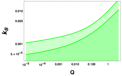
(a) Linear dissipation case.

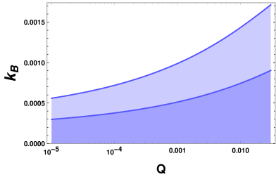
(b) Cubic dissipation case.

Figure 1: $k_{B}$ confidence bounds at 1-$\sigma$ (dark colour) and 2-$\sigma$ (light colour).

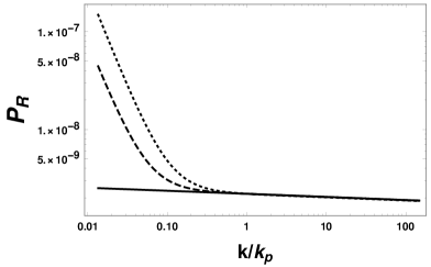
(a) Linear dissipation case.

(b) Cubic dissipation case.

Figure 2: The amplitude of the spectrum as a function of $k/k_{p}$, where $k_{p}$ is the pivot scale, $k_{p}=0.002$ Mpc^-1. The linear dissipative regime is for the case with $Q_{*}=1.02$, while the cubic dissipative regime is for $Q_{*}=0.006$. The solid line corresponds to the WI model without the LQC correction ($\delta_{PL}=0$), the dashed line corresponds to the case including LQC corrections for the $k_{B}$ maximum allowed in this model at 1-$\sigma$ level. The dotted line for the $k_{B}$ maximum allowed at 2-$\sigma$ level.

In order to further see the effects of the WI+LQC in the observables, we show the primordial power spectrum of WI+ LQC for two particular models considered in table 2. In fig. 2 we have thus chosen to use the model with $Q_{*}=1.02$ for the linear dissipative regime, shown in the panel (a), and the case with $Q_{*}=0.006$ for the cubic dissipative regime, shown in the panel (b). We can note that WI with LQC correction (dashed and dotted lines, respectively, obtained using the upper limit values of $k_{B}$ at 1-$\sigma$ and at 2-$\sigma$) increases the power at lower values of $k$, i.e., for large scales, with respect to the simplest WI model (solid line). This behavior is also clear in fig. 3, where we show the temperature anisotropy power spectrum of CMB for the the best fit model values, for the same cases as before, with respect to the CI+LQC model. For the $k_{B}$ parameter, we use the values obtained at 1-$\sigma$ and at 2-$\sigma$ that were reported in table 1 and table 2, for the CI+LQC and WI+LQC cases, respectively. We can note the lower power at low multipoles of the WI+LQC models with respect to the CI+LQC case . The LQC correction to the primordial spectrum thus tends to produce more power at low multipoles of CMB the larger is $k_{B}$ . Taking into account the lower sensitivity of the data in such a region, the differences between the spectra using the best fit values do not lead to a significant difference in the $\chi^{2}$ values, they are about the same in all the cases considered and, thus, we are not showing them explicitly here. Hence, despite the non-trivial modifications in the power spectrum due to the presence of dissipation in addition to the presence of a pre-inflationary dynamics from LQC, our analysis shows that the WI model can explain the current observables also in the context of LQC. At the same time, we can see bounds on the $k_{B}$ value from the LQC correction to the spectra that allow for a larger variation (or freedom) than in the case of CI+LQC.

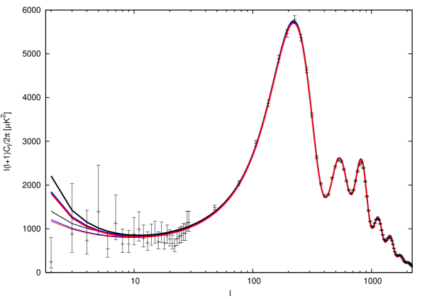
Figure 3: CMB temperature anisotropy power spectrum for the best fit models of WI+LQC in the linear dissipation regime with $Q_{*}=1.02$ (blue lines) and for the cubic dissipative regime with $Q_{*}=0.006$ (red lines), with respect to the CI+LQC model (black line). The models where it was assumed the $k_{B}$ parameter in its 1-$\sigma$ values are draw with the thinner lines, while the thicker ones refer to 2-$\sigma$ values.

4 Conclusions

In this work we have considered the warm inflationary scenario in the context of LQC. The modifications in the standard spectrum due to the pre-inflationary dynamics of LQC and also due to the presence of dissipation during inflation, were examined in the light of the legacy Planck data (2015).

A noteworthy result we get in our analysis is that the upper limit in the value of the LQC parameter scale $k_{B}$ increases with the value of the dissipative ratio $Q_{*}$ in both dissipative regimes that we have analyzed in this paper. Let us recall that models with higher values of $Q_{*}$ ($Q_{*}\gg 1$) have the potential advantage of allowing sub-Planckian initial values for the inflaton field excursion in the WI scenario [75]. Correspondingly, this would lead to models which allow higher values of the LQC parameter scale $k_{B}$, pushing the bounce point closer to the point $N_{*}$ where the relevant physical scales crossed the Hubble radius in the universe history. By making the quantum bounce happen closer to $N_{*}$, it can potentially make it be observable through future CMB precision measurements.

We found that in WI, the bounce can happen at least $\delta N_{*}\geq 17$ e-folds before $N_{*}$ and the modifications in the perturbation spectra still to be consistent with the recent observations. This result can be compared with the one obtained for CI in LQC, $\delta N_{*}\geq 21$. An additional result obtained from our analysis is that models with higher dissipation requires smaller $\delta N$ values. Therefore, WI in LQC requires less extra number of e-folds than CI in LQC. Since it has been suggested in the literature [75] that models with higher values of dissipation can be viable (see also ref. [76] for a recent explicit realization of such a WI scenario), this opens the possibility for a much closer beginning for the quantum bounce in these WI models.

5 Acknowledgements

M.B. acknowledge INFN Sez. di Napoli (Iniziativa Specifica QGSKY) for financial support. L.L.G. acknowledge financial support of the Fundação Carlos Chagas Filho de Amparo á Pesquisa do Estado do Rio de Janeiro (FAPERJ). R.O.R. is partially supported by research grants from Conselho Nacional de Desenvolvimento Científico e Tecnológico (CNPq), Grant No. 302545/2017-4, and Fundação Carlos Chagas Filho de Amparo à Pesquisa do Estado do Rio de Janeiro (FAPERJ), Grant No. E-26/202.892/2017. We acknowledge the use of the High Performance Computing Center at the Universidade Federal do Rio Grande do Norte - NPAD/UFRN - for providing the computational facilities to run our analysis and also the National Observatory of Rio de Janeiro (ON) for the computational support.

References

- [1] N. Aghanim et al. [Planck Collaboration], Planck 2015 results. XI. CMB power spectra, likelihoods, and robustness of parameters, Astron. Astrophys. 594, A11 (2016)
- [2] C. L. Bennett et al. [WMAP Collaboration], Nine-Year Wilkinson Microwave Anisotropy Probe (WMAP) Observations: Final Maps and Results, Astrophys. J. Suppl. 208, 20 (2013)
- [3] D. S. Aguado et al. [SDSS Collaboration], The Fifteenth Data Release of the Sloan Digital Sky Surveys: First Release of MaNGA Derived Quantities, Data Visualization Tools and Stellar Library, [arXiv:1812.02759 [astro-ph.CO]].
- [4] I. Paris et al. [SDSS Collaboration], The Sloan Digital Sky Survey Quasar Catalog: Fourteenth data release, Astron. Astrophys. 613, A51 (2018)
- [5] D. M. Scolnic et al., The Complete Light-curve Sample of Spectroscopically Confirmed SNe Ia from Pan-STARRS1 and Cosmological Constraints from the Combined Pantheon Sample, Astrophys. J. 859, no. 2, 101 (2018)
- [6] K. S. Dawson et al. [BOSS Collaboration], “The Baryon Oscillation Spectroscopic Survey of SDSS-III,” Astron. J. 145, 10 (2013)
- [7] J. E. Bautista et al., “The SDSS-IV extended Baryon Oscillation Spectroscopic Survey: Baryon Acoustic Oscillations at redshift of 0.72 with the DR14 Luminous Red Galaxy Sample,” Astrophys. J. 863, 110 (2018)
- [8] S. H. Suyu et al., “H0LiCOW – I. H0 Lenses in COSMOGRAIL’s Wellspring: program overview,” Mon. Not. Roy. Astron. Soc. 468, no. 3, 2590 (2017)
- [9] T. M. C. Abbott et al. [DES Collaboration], “Dark Energy Survey year 1 results: Cosmological constraints from galaxy clustering and weak lensing,” Phys. Rev. D 98, no. 4, 043526 (2018)
- [10] N. Martinet et al. [Euclid Collaboration], “Euclid Preparation IV. Impact of undetected galaxies on weak-lensing shear measurements,” Astron. Astrophys. 627, A59 (2019)
- [11] P. A. R. Ade et al. [Planck Collaboration], “Planck 2015 results. XXVII. The Second Planck Catalogue of Sunyaev-Zeldovich Sources,” Astron. Astrophys. 594, A27 (2016)
- [12] F. De Bernardis et al., “Detection of the pairwise kinematic Sunyaev-Zel’dovich effect with BOSS DR11 and the Atacama Cosmology Telescope,” JCAP 1703, no. 03, 008 (2017)
- [13] B. P. Abbott et al. [LIGO Scientific and Virgo Collaborations], “Observation of Gravitational Waves from a Binary Black Hole Merger,” Phys. Rev. Lett. 116, no. 6, 061102 (2016)
- [14] B. P. Abbott et al. [LIGO Scientific and Virgo Collaborations], “GW170817: Observation of Gravitational Waves from a Binary Neutron Star Inspiral,” Phys. Rev. Lett. 119, no. 16, 161101 (2017)
- [15] B. P. Abbott et al. [LIGO Scientific and Virgo and Fermi-GBM and INTEGRAL Collaborations], “Gravitational Waves and Gamma-rays from a Binary Neutron Star Merger: GW170817 and GRB 170817A,” Astrophys. J. 848, no. 2, L13 (2017)
- [16] R. A. Sunyaev and Y. B. Zeldovich, Small scale fluctuations of relic radiation, Astrophys. Space Sci. 7, 3 (1970).
- [17] P. J. E. Peebles and J. T. Yu, Primeval adiabatic perturbation in an expanding universe, Astrophys. J. 162, 815 (1970).
- [18] V. Mukhanov and G. Chibisov, Quantum Fluctuation And Nonsingular Universe. (In Russian), JETP Lett. 33, 532 (1981) [Pisma Zh. Eksp. Teor. Fiz. 33, 549 (1981)].
- [19] W. H. Press, Spontaneous Production of the Zeldovich Spectrum of Cosmological Fluctuations, Phys. Scripta 21, 702 (1980).
- [20] Y. Akrami et al. [Planck Collaboration], “Planck 2018 results. X. Constraints on inflation,” arXiv:1807.06211 [astro-ph.CO].
- [21] D. Lyth and A. Liddle, The Primordial Density Perturbation: Cosmology, Inflation and the Origin of Structure, Cambridge University Press, Cambridge, (2009).
- [22] A. Berera, Warm inflation, Phys. Rev. Lett. 75, 3218 (1995) [astro-ph/9509049].
- [23] A. Berera, I. G. Moss and R. O. Ramos, Warm Inflation and its Microphysical Basis, Rept. Prog. Phys. 72, 026901 (2009).
- [24] M. Bastero-Gil and A. Berera, Warm inflation model building, Int. J. Mod. Phys. A 24, 2207 (2009), arXiv:0902.0521.
- [25] A. N. Taylor and A. Berera, Perturbation spectra in the warm inflationary scenario, Phys. Rev. D 62, 083517 (2000).
- [26] L. M. H. Hall, I. G. Moss and A. Berera, Scalar perturbation spectra from warm inflation, Phys. Rev. D 69, 083525 (2004).
- [27] C. Graham and I. G. Moss, Density fluctuations from warm inflation, JCAP 07 013 (2009).
- [28] M. Bastero-Gil, A. Berera and R. O. Ramos, Shear viscous effects on the primordial power spectrum from warm inflation, JCAP 07 030 (2011).
- [29] M. Bastero-Gil, A. Berera, I. G. Moss and R. O. Ramos, Cosmological fluctuations of a random field and radiation fluid, JCAP 1405, 004 (2014).
- [30] S. Bartrum, M. Bastero-Gil, A. Berera, R. Cerezo, R. O. Ramos and J. G. Rosa, The importance of being warm (during inflation), Phys. Lett. B 732, 116 (2014)
- [31] M. Bastero-Gil, A. Berera, R. O. Ramos and J. G. Rosa, Observational implications of mattergenesis during inflation, JCAP 1410, no. 10, 053 (2014)
- [32] M. Bastero-Gil, A. Berera, I. G. Moss and R. O. Ramos, Theory of non-Gaussianity in warm inflation, JCAP 12 008 (2014).
- [33] L. Visinelli, Cosmological perturbations for an inflaton field coupled to radiation, JCAP 1501, no. 01, 005 (2015).
- [34] R. O. Ramos and L. A. da Silva, Power spectrum for inflation models with quantum and thermal noises, JCAP 1303, 032 (2013).
- [35] M. Benetti and R. O. Ramos, Warm inflation dissipative effects: predictions and constraints from the Planck data, Phys. Rev. D 95, no. 2, 023517 (2017)
- [36] N. Bodendorfer, An elementary introduction to loop quantum gravity, [arXiv:1607.05129 [gr-qc]] (2016).
- [37] D. W. Chiou, Loop Quantum Gravity, Int. J. Mod. Phys. D 24, no. 01, 1530005 (2014).
- [38] A. Ashtekar and P. Singh, Loop Quantum Cosmology: A Status Report, Class. Quant. Grav. 28, 213001 (2011).
- [39] A. Barrau, T. Cailleteau, J. Grain and J. Mielczarek, Observational issues in loop quantum cosmology, Class. Quant. Grav. 31, 053001 (2014).
- [40] I. Agullo and P. Singh (2016) Loop Quantum Cosmology, [arXiv:1612.01236 [gr-qc]].
- [41] A. Ashtekar, T. Pawlowski and P. Singh, Quantum nature of the big bang, Phys. Rev. Lett. 96, 141301 (2006).
- [42] A. Ashtekar, T. Pawlowski and P. Singh, Quantum nature of the Big Bang: Improved dynamics, Phys. Rev. D74, 084003 (2006).
- [43] A. Ashtekar, A. Corichi and P. Singh, Robustness of key features of loop quantum cosmology, Phys. Rev. D 77, 024046 (2008).
- [44] I. Agullo, N. A. Morris, Detailed analysis of the predictions of loop quantum cosmology for the primordial power spectra, Phys. Rev. D 92, 124040 (2015).
- [45] I. Agullo, A. Ashtekar, and W. Nelson, Extension of the quantum theory of cosmological perturbations to the Planck era, Phys. Rev. D 87, 043507 (2013).
- [46] I. Agullo, A. Ashtekar, and W. Nelson, Quantum Gravity Extension of the Inflationary Scenario, Phys. Rev. Lett. 109, 251301 (2012).
- [47] I. Agullo, A. Ashtekar, and W. Nelson, The pre- inflationary dynamics of loop quantum cosmology: confronting quantum gravity with observations, Class. Quantum Grav. 30, 085014 (2013).
- [48] A. Ashtekar, W. Kaminski, and J. Lewandowski, Quantum field theory on a cosmological, quantum space-time, Phys. Rev. D 79 (2009) 064030.
- [49] R. Herrera, Warm inflationary model in loop quantum cosmology, Phys. Rev. D 81, 123511 (2010)
- [50] K. Xiao and J. Y. Zhu, A Phenomenology analysis of the tachyon warm inflation in loop quantum cosmology, Phys. Lett. B 699, 217 (2011).
- [51] X. M. Zhang and J. Y. Zhu, Warm inflation in loop quantum cosmology: a model with a general dissipative coefficient, Phys. Rev. D 87, no. 4, 043522 (2013).
- [52] R. Herrera, M. Olivares and N. Videla, General dissipative coefficient in warm intermediate inflation in loop quantum cosmology in light of Planck and BICEP2, Int. J. Mod. Phys. D 23, no. 10, 1450080 (2014).
- [53] S. Basilakos, V. Kamali and A. Mehrabi, Measuring the effects of Loop Quantum Cosmology in the CMB data, Int. J. Mod. Phys. D 26, no. 12, 1743023 (2017).
- [54] A. Jawad, N. Videla and F. Gulshan, Dynamics of warm power-law plateau inflation with a generalized inflaton decay rate: predictions and constraints after Planck 2015, Eur. Phys. J. C 77, no. 5, 271 (2017).
- [55] V. Kamali, S. Basilakos, A. Mehrabi, Meysam Motaharfar and E. Massaeli, Tachyon warm inflation with the effects of Loop Quantum Cosmology in the light of Planck 2015, Int. J. Mod. Phys. D 27, no. 05, 1850056 (2018).
- [56] L. L. Graef and R. O. Ramos, Probability of Warm Inflation in Loop Quantum Cosmology, Phys. Rev. D 98, no. 2, 023531 (2018).
- [57] Suzana Bedic, Gregory Vereshchagin, Probability of inflation in Loop Quantum Cosmology, Phys. Rev. D 99, 043512 (2019).
- [58] T. Zhu, A. Wang, G. Cleaver, K. Kirsten and Q. Sheng, Pre-inflationary universe in loop quantum cosmology, Phys. Rev. D 96, no. 8, 083520 (2017).
- [59] K. A. Meissner, Black hole entropy in loop quantum gravity, Class. Quant. Grav. 21, 5245 (2004).
- [60] A. Ashtekar and D. Sloan, Probability of Inflation in Loop Quantum Cosmology, Gen. Rel. Grav. 43, 3619 (2011).
- [61] L. Parker, Particle creation in expanding universes, Phys. Rev. Lett. 21, 562 (1968); L. Parker, Quantized fields and particle creation in expanding universes. 1., Phys. Rev. 183, 1057 (1969).
- [62] R. Brandenberger, Q. Liang, R. O. Ramos and S. Zhou, Fluctuations through a Vibrating Bounce, Phys. Rev. D 97, no. 4, 043504 (2018).
- [63] E. Wilson-Ewing, Testing loop quantum cosmology, Comptes Rendus Physique 18, 207 (2017).
- [64] M. Bastero-Gil, A. Berera and R. O. Ramos, Dissipation coefficients from scalar and fermion quantum field interactions, JCAP 1109, 033 (2011).
- [65] M. Bastero-Gil, A. Berera, R. O. Ramos and J. G. Rosa, General dissipation coefficient in low-temperature warm inflation, JCAP 1301, 016 (2013).
- [66] M. Bastero-Gil, A. Berera, R. O. Ramos and J. G. Rosa, Warm Little Inflaton, Phys. Rev. Lett. 117, no. 15, 151301 (2016).
- [67] P. A. R. Ade et al. (Planck Collaboration), Planck 2015 results. XX. Constraints on inflation, Astron. Astrophys. 594, A20 (2016).
- [68] M. Bastero-Gil, S. Bhattacharya, K. Dutta and M. R. Gangopadhyay, “Constraining Warm Inflation with CMB data,” JCAP 1802, no. 02, 054 (2018)
- [69] R. Arya, A. Dasgupta, G. Goswami, J. Prasad, and R. Rangarajan, Revisiting CMB constraints on warm inflation, J. Cosmol. Astropart. Phys. 02 (2018) 043, arXiv:1710.11109.
- [70] Wolfram Research, Inc., Mathematica, Version 12.0, Champaign, IL (2019).
- [71] A. Lewis, A. Challinor, and A. Lasenby, Efficient Computation of CMB anisotropies in closed FRW models, Astrophys. J. 538, 473 (2000).
- [72] A. Lewis and S. Bridle, Cosmological parameters from CMB and other data: A Monte Carlo approach, Phys. Rev. D 66, 103511 (2002).
- [73] P. A. R. Ade et al. [BICEP2 and Planck Collaborations], Joint Analysis of BICEP2/Keck Array and Planck Data, Phys. Rev. Lett. 114, 10, 101301 (2015).
- [74] P. A. R. Ade et al. [BICEP2 and Keck Array Collaborations], Improved Constraints on Cosmology and Foregrounds from BICEP2 and Keck Array Cosmic Microwave Background Data with Inclusion of 95 GHz Band, Phys. Rev. Lett. 116, 031302 (2016).
- [75] M. Motaharfar, V. Kamali, R. O. Ramos, Warm inflation as a way out of the swampland, Phys. Rev. D 99, 063513 (2019).
- [76] M. Bastero-Gil, A. Berera, R. O. Ramos and J. G. Rosa, Towards a reliable effective field theory of inflation, arXiv:1907.13410 [hep-ph].