Fundamental parameters and evolutionary status of the magnetic chemically peculiar stars HD 188041 (V1291 Aquilae), HD 111133 (EP Virginis), and HD 204411. Spectroscopy versus interferometry.

Abstract

The determination of fundamental parameters of stars is one of the main tasks of astrophysics. For magnetic chemically peculiar stars, this problem is complicated by the anomalous chemical composition of their atmospheres, which requires special analysis methods. We present the results of the effective temperature, surface gravity, abundance and radius determinations for three CP stars HD 188041, HD 111133, and HD 204411. Our analysis is based on a self-consistent model fitting of high-resolution spectra and spectrophrotometric observations over a wide wavelength range, taking into account the anomalous chemical composition of atmospheres and the inhomogeneous vertical distribution for three chemical elements: Ca, Cr, and Fe. For two stars, HD 188041 and HD 204411, we also performed interferometric observations which provided us with the direct estimates of stellar radii. Comparison of the radii determined from the analysis of spectroscopic/spectrophotometric observations with direct measurements of the radii by interferometry methods for seven CP stars shows that the radii agree within the limits of measurement errors, which proves indirect spectroscopic analysis capable of proving reliable determinations of the fundamental parameters of fainter Ap stars that are not possible to study with modern interferometric facilities.

1 Introduction

Magnetic chemically peculiar (Ap) stars represent a group of stars of spectral types B5 to F5 with global magnetic fields varying from few tens of Gauss (Aurière et al., 2007) to tens of kiloGauss (see catalogue Romanyuk & Kudryavtsev, 2008). Magnetic fields have predominantly poloidal structure. While the Ap stars seem to have the same temperature, mass, luminosity and hydrogen line profiles as the normal Main Sequence (MS) stars, they show atmospheric abundance anomalies. As a rule, element abundance excess of up to 1-4 orders of magnitude compared to the solar abundances is observed for elements heavier than oxygen, while light elements, He, C, N, and O, are underabundant relative to the solar values (see review Ryabchikova, 1991).

Michaud (1970) proposed a mechanism of macroscopic diffusion for developing abundance anomalies in the atmospheres of CP stars. In their atmospheres the diffusion of atoms and ions of a chemical element occurs under the combined action of gravitational settling and the radiation pressure that act in opposite directions. If the gravitational pressure prevails, then the elements diffuse into the deep layers of the atmosphere of the star. In the opposite case, we have a directed flux of particles in the upper atmosphere. The drift of particles occurs with respect to the buffer gas, hydrogen. The element separation results in the creation of vertical abundance gradients that produce the observed abundance anomalies. It changes the atmospheric structure via the line and continuum opacities, which leads to the change of the observed energy distribution compared to the chemically normal stars. Therefore the standard photometric and spectroscopic calibrations developed for the determination of fundamental parameters in normal stars are often inapplicable in case of Ap stars. In Ap stars, the presence of significant individual anomalies of the chemical composition requires the detailed study of stellar chemistry to construct an adequate model atmosphere that can predict the observed flux distribution. Self-consistent procedure of simultaneous spectrum and flux distribution modelling was first proposed by Kochukhov et al. (2009) for one of the brightest Ap stars $\alpha$ Cir. Then it was applied to a few other Ap stars (Shulyak et al., 2009, 2010a; Pandey et al., 2011; Shulyak et al., 2013; Nesvacil et al., 2013). The success of the proposed procedure was verified by the direct measurements of stellar radii in five Ap stars by means of interferometry (Bruntt et al., 2008, 2010; Perraut et al., 2011, 2013, 2016).

In this paper we extend the detailed self-consistent spectroscopic analysis to three other Ap stars, HD 188041 (V1291 Aquilae), HD 111133 (EP Virginis), and HD 204411. For two of them, HD 188041 and HD 204411, we performed interferometric observations and derived their radii. Spectroscopic observations and their analysis are presented in Section 3, and interferometric analysis is given in Section 5.

2 Previous analysis

The investigated objects HD 188041 (V1291 Aquilae), HD 111133 (EP Virginis), and HD 204411 are well-studied Ap stars of spectral class A1 SrCrEu, A6 SrCrEu, and A6 SrCrEu respectively (Renson & Manfroid, 2009). The most anomalous element in their atmospheres is chromium and many of rare-earth elements (REE) which is typical signature of Ap stars (Ryabchikova et al., 2004).

Fundamental parameters ($T_{\rm eff}$, log ${g}$) of the investigated stars were derived in numerous studies in the past using different methods. Netopil et al. (2008) (see the references therein) compiled effective temperature determinations for different groups of chemically peculiar stars. Evolutionary state of Ap stars was studied by Kochukhov & Bagnulo (2006) who derived effective temperatures and luminosities of 150 stars using the calibrations of Geneva photometry and improved Hipparcos parallaxes (van Leeuwen, 2007). These data allow us to estimate stellar radii as well. Both investigations include our program stars. HD 111133 and HD 188041 were analysed for Ca isotopic anomaly and stratification by Ryabchikova et al. (2008), where atmospheric parameters $T_{\rm eff}$  and log ${g}$  were also determined. For HD 204411 fundamental parameters were derived from detailed spectroscopic and stratification study (Ryabchikova et al., 2005) using high-resolution SARG spectrum and Adelman’s spectrophotometry (Adelman et al., 1989). The authors used Hipparcos parallax $\pi=8.37(53)$ mas (ESA, 1997). Position of HD 204411 on the H-R diagram shows that the star finished its main-sequence life. Although being detailed, the spectroscopic analysis of HD 204411 was not fully self-consistent. Previous determinations of fundamental parameters of program stars are collected in Table 1. Here and throughout the paper an error of the measurement in the last digits is given in parentheses.

Table 1: Literature data for the fundamental parameters of program stars.

HD	$T_{\rm eff}$	log ${g}$	$\log(L/L_{\odot})$	$R/R_{\odot}$	Ref.
	9850(220)				Netopil et al. (2008)
HD 111133	9930(250)		1.92(13)	3.09	Kochukhov & Bagnulo (2006)
	9930	3.65			Ryabchikova et al. (2008)
	8580(550)				Netopil et al. (2008)
HD 188041	8430(200)		1.55(07)	2.80	Kochukhov & Bagnulo (2006)
	8800	4.00			Ryabchikova et al. (2008)
	8510(170)				Netopil et al. (2008)
HD 204411	8750(300)		1.95(06)	4.12	Kochukhov & Bagnulo (2006)
	8400(200)	3.50(10)	2.01(10)	4.6(2)	Ryabchikova et al. (2005)

In this work we extend the analysis of these stars by employing self-consistent abundance and stratification study based on dedicated model atmospheres and available spectroscopic and (spectro-)photometric observations, as described below.

3 Spectroscopy

3.1 Observations

High-resolution spectra of HD 111133 and HD 188041 were obtained with the UV-Visual Echelle Spectrograph (UVES) attached at the ESO VLT (program ID 68.D-0254). The resolving power of the spectrograph is R=$\lambda/\Delta\lambda$=80 000, spectral region covered is 3100 to 10000 Å. Details of the observations and data processing are given in Ryabchikova et al. (2008). HD 204411 was analysed using an echelle spectrum (R=164 000, spectral region 4600–7900 Å) obtained with the high resolution spectrograph (SARG) attached to the 3.55-m Telescopio Nazionale Galileo at the Observatorio del Roque de los Muchachos (La Palma, Spain). A detailed description of the data and data processing is given in Ryabchikova et al. (2005).

3.2 Self-consistent spectroscopic analysis

To accurately derive fundamental parameters – effective temperature, surface gravity, radius, and luminosity – of a magnetic CP star we applied an iterative method proposed by Kochukhov et al. (2009) for the roAp star $\alpha$ Cir and then used for few other Ap stars (see Section 1). Briefly, the basic steps of this method include the repeated stratification and abundance analysis used in the calculations of model atmosphere and theoretical SED which is compared to the observed one. SED fit also allows to estimate stellar radius provided that the stellar parallax is known. Iterations continue until fundamental parameters ($T_{\rm eff}$, log ${g}$, $R$, chemistry) used in SED fitting converge. Thus, we get abundance pattern which is consistent with the physical parameters of the final stellar atmosphere. Model atmosphere calculations were done with the LLmodels code (Shulyak et al., 2004). As starting parameters in iteration procedure, we used model parameters from Ryabchikova et al. (2008) for HD 111133, HD 118041 and from Ryabchikova et al. (2005) for HD 204411. The details of our SED analysis will be given in Sect. 4 and below we only describe the steps of our self-consistent spectroscopic analysis.

3.2.1 Abundance analysis

The abundances of chemical elements were evaluated using two different methods. Here and everywhere element abundance is given as $\log(N_{el}/N_{tot})$, where $N_{el}$ is a number of atoms of a considered element and $N_{tot}$ is a total number of atoms. A fast method of element abundance determination uses measured equivalent widths of the corresponding spectral lines. For that we utilized the widthV code (Ryabchikova et al., 2002). However, it is difficult to apply simple equivalent widths calculations to magnetic stars due to magnetic splitting and intensification of spectral lines. Therefore, a special version of the widthV code called WidSyn was developed (Shulyak et al., 2013). The program provides an interface to magnetic spectrum synthesis code SYNMAST (for a more detailed description see Kochukhov, 2007; Kochukhov et al., 2010) where theoretical equivalent widths are calculated from the full polarized radiative transfer spectrum synthesis. We assumed surface magnetic field to be constant with depth and defined by radial and meridian components of magnetic field vector whose modulus $\langle B_{\rm s}\rangle$ is derived from the magnetic splitting of spectral lines in nonpolarized observed spectrum. The observed $\langle B_{\rm s}\rangle$ values are taken from Ryabchikova et al. (2008) for HD 111133 and HD 188041, from Ryabchikova et al. (2005) for HD 204411 and are given in Table 5. Line atomic parameters were extracted from the Vienna Atomic Line Database VALD (Kupka et al., 1999) in its 3d release VALD3 (Ryabchikova et al., 2015).

Another, more accurate method to measure element abundance is based on a direct fitting of the theoretical profiles of individual spectral lines by varying parameters $v_{\rm e}\sin i$, $V_{\rm r}$ (stellar projected rotation and radial velocity, respectively), two components of the magnetic field vector, and element abundance. It was done with SYNMAST code implemented in the visualization program BinMag6 (Kochukhov, 2018). The direct spectrum synthesis takes into account possible blends, since the lines are often blended in spectra of CP stars, and the abundance estimation by equivalent widths may not be very accurate. We performed a comparative analysis of the Fe (HD 111133) and Nd (HD 188041) abundances derived by both methods using 23 Fe i, ii lines and 11 Nd iii lines. Figure 1 shows this comparison for Fe lines. Due to the careful choice of spectral lines the abundances derived by both methods agree rather well. The corresponding Fe abundance is -3.26(29) (WidSyn) versus -3.26(26) (SYNMAST). A similar satisfactory agreement was obtained for Nd abundance.

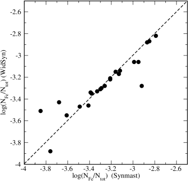
Figure 1: Comparison between Fe abundances derived from the equivalent widths (WidSyn code) and by magnetic spectrum fitting (SYNMAST code).

Based on the results of our investigation we prefer to use equivalent width method for abundance analysis in most cases. The mean atmospheric abundances of 36 elements were derived at each iteration. For 17 elements this was done using spectral lines of two ionization stages. The isotopic structure of Ba II and Eu II was taken into account, however we neglected the hyperfine splitting (hfs) because of the complex interaction between the hyperfine and magnetic splittings (Landi Degl’Innocenti, 1975). It means that abundances of a few elements with the odd isotopes (Mn, Co, Pr, Eu, Tb) may be overestimated. The only exception is HD 204411 where we neglected the magnetic field in abundance analysis. For this star we employed profile fitting method when necessary and used hfs data from Blackwell-Whitehead et al. (2005); Holt et al. (1999) (Mn i,  ii), Pickering (1996) (Co i), Villemoes et al. (1993) (Ba ii).

Average abundances for the final atmospheric models are given in Table 2. Model parameters are presented in Section 4.2. The last column of the table presents the current solar photospheric abundances (Asplund et al., 2009; Scott et al., 2015a; Scott et al., 2015b; Grevesse et al., 2015).

Table 2: The mean values of chemical abundance $\log(N_{el}/N_{tot})$, calculated from equivalents widths of N lines for model atmospheres 8770g42 (HD 188041), 9800g40 (HD 1111333), and 8300g36 (HD 204411). Values derived from one line are marked with a colon. The standard deviation is given in parentheses. Solar photospheric abundances are given in the last column.

Ion	Abundance $\log(N_{el}/N_{tot})$
	HD 188041	N	HD 111133	N	HD 204411	N	Sun
C i	-4.17(29)	3	-4.25(54)	3	-4.48(15)	5	-3.61
N i	-4.94(25)	2	-5.10:	1	-4.15(05)	2	-4.21
O i	-4.60(36)	4	-3.93(43)	7	-3.71(07)	4	-3.35
Na i	-5.62(15)	2	-5.68(70)	2	-5.63(07)	2	-5.83
Mg i	-4.34(80)	2	-4.42(18)	4	-4.60(20)	6	-4.45
Mg ii	-4.28(13)	2	-4.49(52)	5	-4.62(49)	3	-4.45
Al i	-4.50:	1					-5.61
Al ii	-4.57(13)	2	-5.90(01)	2			-5.61
Si i	-3.90(19)	5	-4.09(60)	9	-4.33(15)	6	-4.53
Si ii			-4.65(35)	4	-4.12(03)	2	-4.53
S i	-3.44:	1			-5.12(23)	2	-4.92
S ii			-5.09(50)	3			-4.92
Ca i	-4.69(58)	11	-5.98:	1	-5.54(05)	5	-5.72
Ca ii	-4.96(32)	2	-6.87(20)	3	-5.05(11)	5	-5.72
Sc ii	-8.32(70)	5			-9.68:	1	-8.88
Ti i					-6.81(11)	13	-7.11
Ti ii	-6.45(54)	14	-6.51(42)	29	-6.63(11)	15	-7.11
V i	-5.60(23)	2					-8.15
V ii	-6.80(47)	6	-8.05(19)	9	-8.87(09)	2	-8.15
Cr i	-3.97(57)	10	-3.71(31)	66	-5.18(16)	37	-6.42
Cr ii	-3.81(54)	15	-3.88(43)	248	-4.90(19)	36	-6.42
Mn i	-4.94(62)	9	-4.96(28)	9	-6.25(13)	9	-6.62
Mn ii	-4.99(88)	5	-4.97(39)	51	-5.91(18)	14	-6.62
Fe i	-3.60(35)	19	-3.24(27)	153	-4.10(20)	79	-4.57
Fe ii	-3.21(40)	52	-3.24(32)	282	-3.64(34)	69	-4.57
Co i	-5.05(63)	9	-5.09(47)	14	-6.65(20)	3	-7.11
Co ii	-5.50:	1	-5.48(52)	12
Ni i	-5.81(63)	5	-5.77(76)	10	-5.96(14)	27	-5.84
Ni ii			-6.18(57)	3	-5.42:	1	-5.84
Cu i	-6.88:	1			-8.26:	1	-7.86
Sr i	-5.81:	1			-8.99:	1	-9.21
Sr ii	-5.97(12)	2	-7.07(51)	3			-9.21
Y ii	-9.23(40)	4	-8.83(22)	3	-10.24(14)	4	-9.83
Zr ii	-8.25(57)	10	-8.57(77)	10	-9.12(28)	2	-9.45
Nb ii	-8.09(73)	2					-10.57
Mo ii	-7.72(17)	2					-10.16
Ba ii	-9.12(57)	4	-8.93(39)	3	-9.45(23)	3	-9.79
La ii	-8.29(23)	6	-7.97(60)	18			-10.93
Ce ii	-7.62(31)	14	-7.46(62)	27	-10.46:	1	-10.46
Ce iii	-6.08(35)	6	-7.14(24)	4			-10.46
Pr ii	-7.91(38)	4	-7.90(41)	6			-11.32
Pr iii	-8.47(30)	9	-8.30(43)	25			-11.32
Nd ii	-8.33(56)	3	-7.64(40)	24	-9.80(22)	3	-10.62
Nd iii	-7.87(28)	12	-8.32(44)	33	-10.14:	1	-10.62
Sm  ii	-8.52(30)	6	-8.06(35)	15			-11.09
Sm iii	-7.07:	1	-8.46(04)	2			-11.09
Eu ii	-7.41(24)	5	-8.93(58)	6	-11.19:	1	-11.52
Eu iii	-5.29(53)	4	-6.68(29)	7			-11.52
Gd ii	-7.48(71)	8	-7.38(46)	25			-10.96
Tb ii	-7.91:	1					-11.70
Tb iii	-8.85(36)	4	-8.44(50)	1			-11.70
Dy ii	-8.95(48)	4	-7.88(45)	13			-10.94
Er ii	-9.38(45)	4	-8.20(45)	7			-11.11
Er iii	-8.06:	1	-8.56(56)	5			-11.11
Tm ii	-8.83(1.42)	3	-9.03:	1			-11.93
Yb ii	-8.07(44)	5	-8.09(37)	10			-11.19

Figure 2 shows the mean element abundances in the atmospheres of investigated stars relative to the solar photospheric values. Abundances derived from the lines of consecutive ionization stages (neutral and first ions or first and second ions for REE) are shown by filled and open circles, respectively. The abundances in HD 111133 and HD 188041 are similar within the errors of the determination, and the abundance patterns correspond to the general observed anomalies in Ap-stars: CNO deficiency, practically solar Na and Mg abundance, 1-2 dex overabundance of the iron peak elements, and a large excess of the rare-earth elements (REEs). However, the abundance pattern in HD 204411 is different. CNO deficiency is the same, iron peak elements are less overabundant, and the REEs are close to the solar values. We discuss this issue in Section 6.

Inspecting Table 2 one notices rather large abundance difference derived from the lines of consecutive ionization stages of some elements, e.g. Ca, Cr, Fe, Eu. Usually it may be an indication of abundance stratification in stellar atmosphere (Ryabchikova et al., 2003). There is no significant violation of the ionization equilibrium of those rare-earth elements (Ce, Pr, Nd, Sm) for which the abundance is determined more or less reliably by several lines of different ionization stages. The exception is Eu, where the Eu iii lines provide more than an order of magnitude higher abundance compared to the Eu ii lines. This behaviour is typical for most Ap stars in the effective temperature range of 7000–10000 K (Ryabchikova & Romanovskaya, 2017).

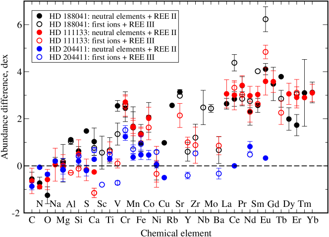
Figure 2: Element abundances relative to solar values in the atmospheres of HD 188041 (black symbols), HD 111133 (red symbols), and HD 204411 (blue symbols). Abundances derived from the lines of the neutral species (C to Ba) and of the first ions (La to Yb) are shown with filled circles, and those derived from the lines of the first (C to Ba) and the second (La to Yb) ions are shown with open circles.

As was mentioned above, some elements may have inhomogeneous vertical distribution, which changes atmospheric structure through the variable line opacity. We performed stratification analysis of iron, chromium and calcium, because the lines of these elements (in particular, Fe and Cr) dominate the observed spectrum.

3.2.2 Stratification study

Element stratification was calculated using the DDaFit IDL-based automatic procedure (Kochukhov, 2007). Theoretical stratification calculations show that, as a first approximation, the stratification profile of chemical elements can be represented by a step function (Babel, 1992). This function is described by four parameters: element abundances in the upper and lower atmospheric layers, the position of the abundance jump and the width of this jump. These parameters are optimized to provide the best fit to the observed profiles of spectral lines formed at different atmospheric layers. Spectral synthesis is carried out with the SYNMAST program, and the possible contribution of neighboring lines is taken into account. The success of the stratification study strongly depends on the choice of spectral lines. The chosen lines should be sensitive to possible abundance variations at significant part of atmospheric layers. The list of the lines is given in Table 3 and is available in electronic version of the paper. Here we present only a part of this table.

Table 3: A list of spectral lines used for the stratification calculations for stars HD 188041, HD 111133, and HD 204411 with the excitation potential (eV), oscillator strength ($\log\,{gf}$) and Stark damping parameter ($\log\,\gamma_{\rm St}$) listed.

Ion	$\lambda$ (Å)	$E_{\textnormal{i}}$ (eV)	$\log\,{gf}$	$\log\gamma_{\rm St}$	HD 188041	HD 111133	HD 204411
Fe II	4504.343	6.219	-3.250	-6.530	$\surd$
Fe II	4508.280	2.855	-2.250	-6.530		$\surd$
Fe II	4610.589	5.571	-3.540	-6.530	$\surd$	$\surd$
Fe II	4631.867	7.869	-1.945	-5.830	$\surd$	$\surd$
Fe II	4975.251	9.100	-1.763	-6.530		$\surd$
Fe II	4976.006	9.100	-1.599	-6.530	$\surd$
Fe I	5014.942	3.943	-0.303	-5.450	$\surd$	$\surd$
Fe II	5018.435	2.891	-1.220	-6.530	$\surd$	$\surd$	$\surd$
Fe II	5018.669	6.138	-4.010	-6.537			$\surd$
Fe I	5019.168	4.580	-2.080	-5.970			$\surd$
……	……	……	……	……	…..	……	……
This table is available in its entirety in a machine-readable form in the online journal. A portion is shown here for guidance regarding its form and content. Stark damping parameters are given for one perturber (electron) for T=10000 K.

Stratification calculations began with the homogeneous abundance distribution corresponding to the average atmospheric abundances derived as described in Section 3.2.1. DDaFit procedure is repeated for each iteration, every time using model atmosphere with improved atmospheric parameters $T_{\rm eff}$, log ${g}$, and abundance patterns which are refined through the fitting of spectral energy distribution (see Section 4.2). In Fig. 3 and Fig. 4 we show final Ca, Cr, and Fe stratifications.

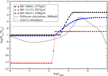
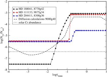
Figure 3: Distribution of Ca (left panel) and Cr (right panel) in the atmospheres of HD 188041 (black filled circles), HD 111133 (red filled circles), and HD 204411 (blue filled circles). Theoretical predictions for the model $T_{\rm eff}$=9000 K, log ${g}$=4.0 are shown by dashed line. Solar abundances are indicated by dotted line.

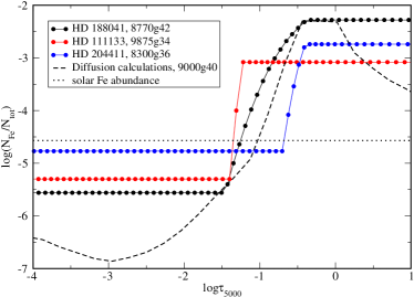
Figure 4: The same as in Fig. 3, but for Fe.

All the three elements have abundance jumps in the atmospheres of investigated stars, and these jumps are located at the optical depths close to the predictions of the diffusion theory. It is demonstrated by the comparison of the empirical stratifications with the theoretical diffusion calculations for model $T_{\rm eff}$=9000 K, log ${g}$=4.0 (Leblanc & Monin, 2005; LeBlanc et al., 2009). However, in the atmosphere of the most evolved star HD 204411 abundance jumps seem to be smaller, in particular, for Cr. All the three stars show large Fe and Cr overabundance in the deep atmospheric layers where high-excitation lines are formed. The most unusual result is Ca deficiency throughout the whole atmosphere of HD 111133, which is not predicted by the diffusion theory.

The results of our analysis do not differ much from the derived Ca stratification in HD 188041 and HD 111133 (Ryabchikova et al., 2008), and from Ca-Cr-Fe stratifications derived by Ryabchikova et al. (2005). It is not surprising because the cited studies were based on the same observed spectra. Stratification analysis allows us to derive more accurately stellar rotational velocities. The best fits of the calculated line profiles to the theoretical ones were obtained for $v_{\rm e}\sin i$=2 km s^-1 in HD 188041 and for $v_{\rm e}\sin i$=6 km s^-1 in HD 111133.

4 Analysis of spectral energy distribution

4.1 Observations

Spectral energy distribution (SED) in absolute units for all the three stars was constructed from UV wide-band fluxes obtained with TD1 space mission and extracted from TD1 catalogue (Thompson et al., 1978), from optical spectrophotometry (Breger, 1976; Adelman et al., 1989), and from the near infrared 2MASS (2Micron All-Sky Survey) catalogue which contains an overview of the entire sky at $J$-band (1.25 $\mu m$), $H$-band (1.65 $\mu m$), and $K$-band (2.17 $\mu m$). The spectrophotometric magnitudes by (Adelman et al., 1989) were converted to fluxes using Vega calibrations given in Hayes & Latham (1975). We convert 2MASS magnitudes to absolute fluxes using filter values and zero points defined in Cohen et al. (2003).

For HD 188041, we additionally utilized fluxes between $1900$ Å and $3000$ Å observed with International Ultraviolet Explorer (IUE).

Along with the low-resolution spectrophotometric data by (Adelman et al., 1989), for HD 204411 we made use of the medium resolution spectroscopic observations with the Boller & Chivens long-slit spectrograph mounted at $2.1$ m telescope at the Observatorio Astronómico Nacional at San Pedro Mártir, Baja California, México (OAN SPM). The data for HD 204411 and several other Ap stars was obtained during July, 2011. In order to make precise spectrophotometry, the slit was opened as wide as possible to cover the star’s photometric profile together with its far wings and surrounding sky background. With this configuration spectral resolution of about $8$ Å and simultaneously registered wavelength range from $3700$ Å to $7200$ Å were achieved.

The wavelength calibration with an arc lamp spectrum obtained several times per the observing night, spectrograph flexion correction, and flat-fielding with a halogen lamp were made in a standard manner. The spectra of the star were flux-calibrated using spectrophotometric standard stars observed at different zenith distances during the same night. In particular case of HD 204411 we used two calibrator stars HD 192281 and BD+33d2642, respectively.

4.2 The determination of fundamental stellar parameters.

To compare the observed and theoretical fluxes at different wavelengths (spectral energy distribution – SED) one needs to calculate irradiation from the surface of a star located at some distance. This irradiation depends on stellar atmospheric parameters, stellar radius, and the distance to the star. The distance is defined by stellar parallax. We compute theoretical fluxes at different wavelengths from the adopted model atmosphere. We optimize stellar radius, $T_{\rm eff}$, and log ${g}$ for a given abundance pattern and stratification to reach the best fit to the observed energy distribution. This approach allows us to refine the atmospheric parameters and the radius of the star simultaneously.

Because we utilize datasets that come from different space and ground-based missions, the number of observed points that we fit can differ from only a few (e.g., 2MASS) to hundreds (e.g., IUE) depending on wavelength domain. Therefore, in order to ensure that each wavelength domain equally contribute to the final fit, we weight data in UV, Visual, and IR spectral ranges by corresponding number of observed points. We chose three weighting regions: $0$-$4200$ÅÅ, $4200$-$11000$ÅÅ, $11000$-$\infty$ÅÅ. The first region is useful for the estimation of stellar gravity because it includes the Balmer jump whose amplitude is sensitive to the atmospheric pressure for stars of early spectral types. The second and the third regions are mostly sensitive to the stellar effective temperature. Altogether, having observations in UV, Visual, and IR helps to constrain accurate atmospheric parameters (Shulyak et al., 2013).

It is known that CP stars exhibit variability of their fluxes with the rotation period as observed in different photometric filters (e.g., Molnar, 1973; Adelman et al., 1989). This variability is caused by non-homogeneous distribution of chemical elements across the stellar surface (abundance spots) which produces stellar brightness variation due to the changes in local atmospheric opacity, as explained in numerous investigations (see, e.g., Krtička et al., 2009; Shulyak et al., 2010b; Krtička et al., 2012; Krtička et al., 2015). Among different observation data sets available to us only Adelman et al. (1989) set contains several scans per star taken at different rotation phases. However, the flux variability in our sample stars reaches maximum of about $12$% in HD 204411, $9$% in HD 188041, and $6$% in HD 111133, respectively. We therefore conclude that abundance spots do not introduce strong biases in our parameters estimation. Note that the amplitude of flux variation is the largest at short wavelengths where the atmospheric opacity is the strongest. Unfortunately, the available UV fluxes provided by the TD1 sattelite do not contain time resolved information. Because in our SED fit we combine data obtained at differench epochs and with different missions and/or instruments we could not study the impact of abundance spots on determination of atmospheric parameters in full detail. Thus, in our analsys we minimize the impact of phase variability of stellar fluxes by averaging individual scans taken by Adelman et al. (1989) for each star.

The parallax values were taken from the second GAIA release DR2 (Gaia Collaboration et al., 2018). Regarding the total uncertainty $\sigma_{\rm ext}$ on each parallax, we have computed it using the formula provided by Lindegren et al. at the IAU colloquium:

$$\sigma_{\rm ext}=\sqrt{k^{2}\sigma_{i}^{2}+\sigma_{s}^{2}}$$ (1)

with $\sigma_{i}$ provided in the GAIA DR2 catalogue, $k$ = 1.08 and $\sigma_{s}$ = 0.021 mas for $G$ < 13. We thus considered the values of 11.72(11) mas (HD 188041), 5.21(07) mas (HD 111133), and 8.33(12) mas (HD 204411), respectively. The adopted parallaxes differ from the original (ESA, 1997) and revised (van Leeuwen, 2007) Hipparcos ones by 5-6 % for HD 188041 and HD 204411, and by more than 30 % for HD 111133. For example, for HD 188041 the available parallax values are 11.79(93) (ESA, 1997), 12.48(36) (van Leeuwen, 2007), 11.95(97) (Gaia Collaboration et al., 2016), and 11.72(10) (Gaia Collaboration et al., 2018), while the corresponding values for HD 111133 are 6.23(93), 3.76(40), 5.95(73), and 5.21(06), respectively. Such a large scatter in parallax values for HD 111133 influences the radius estimate and, hence, the luminosity (see Sections 4.2.2 and 6).

Our three stars are located at the short distance from the Sun, therefore the corrections for interstellar reddening $A_{v}$ are small and were taken to be zero for HD 188041, 0.^m03 for HD 111133, and 0.^m016 for HD 204441. We calculated these values based on the reddening maps from Amôres & Lépine (2005). It corresponds to the E(B-V) values of 0.^m009 (HD 111133) and 0.^m005 (HD 204411) if one takes a typical parameter $R_{v}$=3.1 in standard extinction low. In the last two years new 3D reddening maps were published based on the data from GAIA mission. Table 4 collects E(B-V) data from four different sources: Amôres & Lépine (2005), Lallement et al. (2018), Green et al. (2018), and Gontcharov & Mosenkov (2018). One can easily see rather large dispersion between different sets. Colour excess E(B-V) extracted from the catalogs of Gontcharov & Mosenkov (2018) provide the largest estimates, while the maps of interstellar dust in the Local Arm constructed by Lallement et al. (2018) using Gaia, 2MASS, and APOGEE-DR14 data give us the E(B-V) values not very different from Amores & Lepine. Green et al. (2018) provide a code for E(B-V) calculations in different modes. We chose data calculated in mode ’median’. In order to account for interstellar reddening we used the fm_unred routine from the IDL Astrolib package that uses reddening parameterization after Fitzpatrick (1999).

Table 4: Reddening data for HD 111133, HD 188041 and HD 204411.

HD	d, pc	E(B–V)
		1	2	3	4
HD 111133	191.9(2.1)	0.010	0.017(020)	0.027	0.06(05)
HD 188041	85.3(0.7)	0.000	0.007(017)	0.012	0.10(05)
HD 204411	120.0(1.6)	0.005	0.011(015)	0.028	0.07(05)
1 – Amôres & Lépine (2005), 2 – Lallement et al. (2018), 3 – Green et al. (2018), 4 – Gontcharov & Mosenkov (2018)

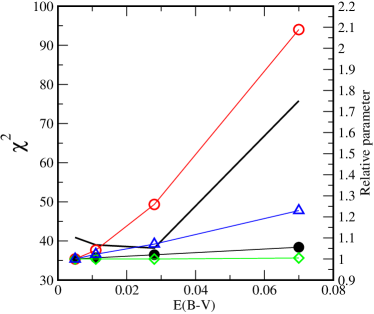
Figure 5: Fundamental stellar parameters of HD 204411 as a function of E(B-V). Black solid line shows $\chi^{2}$ of the SED fit (left y-axis), while variation of the relative values for $T_{\rm eff}$  (black filles circles), log ${g}$  (open red circles), radius (open green diamonds) and luminosity (open blue triangles) are marked on the right y-axis. The reference parameters derived with E(B-V)=0.^m005 are given in Table 5.

We checked SED fitting for all E(B-V) from Table 4. Figure 5 demonstrates the influence of the reddening on the derived stellar parameters $T_{\rm eff}$, log ${g}$, radius and luminosity in HD 204411. The similar picture was obtained for HD 188041. It is evident that our solution for two stars, HD 188041 and HD 204411, with the reddening data from Amôres & Lépine (2005) provides the proper atmospheric parameters, and a slight increase in E(B-V) (first three points in Fig. 5) produces parameter variations within the uncertainties indicated in our work. The largest variations are observed for gravity, but in logarithmic scale it corresponds to the uncertainty 0.1 dex given in Table 5.

However, for HD 111133 the situation is opposite. The best fit to the SED was obtained for the largest reddening, but the observed high resolution spectrum cannot be fit with the atmospheric parameters derived with this reddening values (see Section 4.2.2).

For all stars, models with a solar helium abundance and with the reduced by several orders helium abundance were constructed because the helium deficiency is typical for peculiar stars. Our analysis showed that models with normal helium abundance provide slightly better fit to the observed SED. Final atmospheric parameters and stellar radii are obtained during the iterative process as described in Section 3.2. Five iterations were required to reach the convergence for HD 188041, 3 iterations for HD 111133, and 2 iterations for HD 204411.

4.2.1 HD 188041

Figure  6 shows a comparison between the observed SED and the theoretical calculations for the atmosphere of HD 188041. Using TD1 fluxes in UV wavelength domain we obtained the following best fit parameters: $T_{\rm eff}$=8770(30) K, log ${g}$=4.2, solar helium abundance, and radius $R/R_{\odot}$ = 2.39(2). However, we could not obtain good constraints for the log ${g}$  because our fitting algorithm was always favoring the largest value available in our model grid. On the contrary, when using IUE fluxes we obtained $T_{\rm eff}$=8613(11) K, log ${g}$=4.02(5) K, $R/R_{\odot}$ = 2.44(1) and thus better estimates for the log ${g}$  which agrees with what is expected for A-type main-sequence stars. The lower $T_{\rm eff}$ obtained from fitting IUE flux is because the latter appears to be systematically lower compared to TD1 flux.

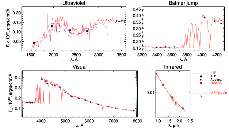
Figure 6: Comparison of the observed energy distribution (black filled squares and diamonds) with the theoretical flux (red solid line) calculated for LLmodels atmosphere of HD 188041 with the parameters $T_{\rm eff}$=8770 K, log ${g}$=4.2. Open blue diamonds show the theoretical fluxes convolved with the corresponding filters. 2MASS photometric colours are presented by filled red squares.

4.2.2 HD 111133

In all attempts to fit the observed SED with E(B-V)$\leq$0.^m03 we could not constrain stellar log ${g}$. Using reddening from Gontcharov & Mosenkov (2018) we got the best $\chi^{2}$ fit, however, model atmosphere with $T_{\rm eff}$=10300 K, log ${g}$=3.17 cannot reproduce hydrogen line profiles and Fe i/Fe ii  lines with any stratification. A detailed analysis carried out for HD 111133 with E(B-V)=0.^m010 –0.^m027 showed slight but not statistically significant improvement of $\chi^{2}$ SED fit with the increase of E(B-V) for two fixed log ${g}$: 4.0 and 3.4. SED fit with fixed log ${g}$=4.0 provides slightly better $\chi^{2}$, however log ${g}$=3.4 is preferred because it fits the hydrogen lines better (see Fig.7).

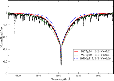
Figure 7: Comparison of the observed H$\alpha$ line profile in HD 111133 (black filled circles) with the synthetic profiles calculated using model atmospheres 9875g34 (red solid line), 9770g40 (dashed green line), and 10300g317 (blue dotted line).

We used parallax 5.21(7) mas in our fitting procedure. As for HD 188041, the model with solar helium abundance fits somewhat better the observed energy distribution. Finally, we chose a model with $T_{\rm eff}$=9875 K, log ${g}$=3.4 derived from SED fit with E(B-V) taken from Amôres & Lépine (2005) as for two other stars. Comparison of the observed fluxes with the theoretical ones is shown in Fig. 8. Note that even after convergence we could not reach a good agreement between the observed and theoretical energy distributions as in the case of HD 188041. This is especially noticeable in the UV spectral region up to the Balmer jump. Ignoring TD1 fluxes we obtained best fit model that is about $100$ K hotter but could not constrain stellar log ${g}$ (not shown on the plot).

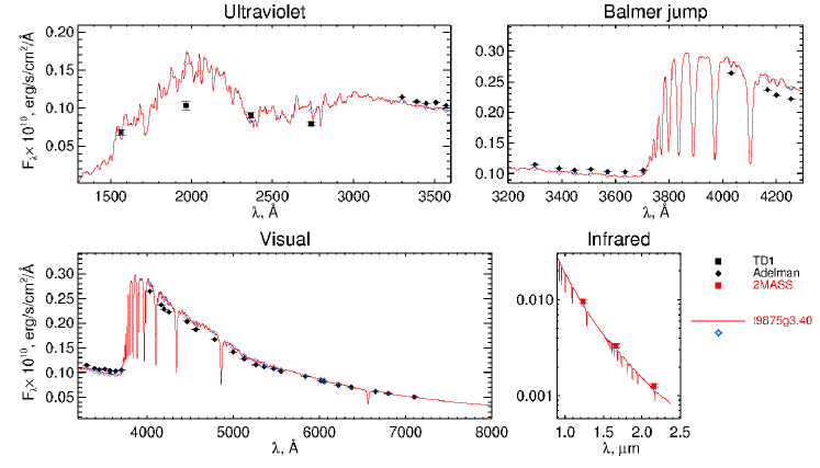
Figure 8: Same as in Fig. 6, but for HD 111133.

Using the largest parallax value of 6.23(93) (ESA, 1997) we derive the same effective temperature and gravity as before, but smaller radius $R/R_{\odot}$=2.92(44) (with the parallax uncertainty taken into account in the error estimate).

4.2.3 HD 204411

We compare the observed and theoretical fluxes for HD 204411 on Fig. 9. We obtained the best fit of the theoretical flux to the observed one after two iterations and for the model with $T_{\rm eff}$=8300(22) K, log ${g}$=3.6(5), $R/R_{\odot}$=4.42(2) using parallax 8.33(12) mas and low resolution spectro-photometry from Adelman et al. (1989). We obtain very similar result if we use spectro-photometry from Breger (1976): $T_{\rm eff}$=8295(30) K, log ${g}$=3.5(6), $R/R_{\odot}$=4.45(3). If we use observations obtained with the Boller & Chivens spectrometer, we obtained very close estimates of $T_{\rm eff}$=8356(11) K, log ${g}$=3.41(4), $R/R_{\odot}$=4.45(1) and $T_{\rm eff}$=8351(10) K, log ${g}$=3.23(4), $R/R_{\odot}$=4.46(1) for the two different calibrators BD+33d2642 and HD 192281, respectively. However, in order to achieve such a good match we had to ignore fluxes blueward $4000$ Å  because of poor sensitivity of the spectrometer at these short wavelengths, as can be seen from Fig. 9.

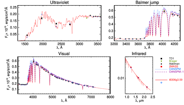
Figure 9: Same as in Fig. 6 but for HD 204411. We also show SEDs obtaiend with the Boller & Chivens long-slit spectrograph (OAN SPM, México) and calibrated to absolute flux units using two different calibrators and marked as OANSPM (calibrator BD+33d2642) and OANSPM-1 (calibrator HD 192281), respectively (see the figure legend).

4.2.4 Adopted fundamental parameters

As was shown above, determination of fundamental parameters relies on datasets obtained with different instruments and missions and for the same star there could be several alternative observations available. Also, our errors on the temperature, gravity, and radius listed above result from the $\chi^{2}$ minimization algorithm and are obviously underestimated because of uncertainties in model atmopsheres, different data sources and accuracy of their calibration, etc. Therefore, we decided to adopt concervative uncertainties that account for the scatter in our estimates. Moreover, because for all our targets we always have data from at least three observing campangs (TD1 for UV, Adelman et al. (1989) for VIS, and 2MASS for IR), we adopted final parameters from the fit to these three data sets, adding the parallax uncertainty to radius estimates: $T_{\rm eff}$=8770(150) K, log ${g}$=4.2(1), $R/R_{\odot}$ = 2.39(5) for HD 188041, $T_{\rm eff}$=9770(200) K, log ${g}$=4.0(2), $R/R_{\odot}$ = 3.49(7) for HD 111133, and $T_{\rm eff}$=8300(150) K, log ${g}$=3.6(1), $R/R_{\odot}$ = 4.42(7) for HD 224411, respectively. The luminosity of stars were calculated from the derived values of the effective temperature and radius. The finally adopted parameters are listed in Table  5. For HD 111133 we provide two sets of parameters based on Hipparcos and GAIA parallaxes, respectively.

Our model SED’s clearly show a presence of 5200Å  depression usually observed in Ap stars. From our theoretical fluxes we computed $\Delta$a-index according to Khan & Shulyak (2007) and found it to be 56 mmag for HD111133, 60 mmag for HD188041, and 20 mmag for HD204411. Theoretical $\Delta$a values agree very well with the observed data: 56 mmag (HD 111133), 60 mmag (HD 188041) and 19 mmag (HD 204411). For the first two stars the observed values are taken from Maitzen (1976), while for HD 204411 $\Delta$a-index is taken from Maitzen et al. (1998). This comparison gives a credit to the results of our modelling.

5 Interferometric observations

The two stars HD 188041 and HD 204411 were observed between June 2015 and June 2017 with the VEGA instrument (Mourard et al., 2009) at the CHARA interferometric array (ten Brummelaar et al., 2005) with the medium spectral resolution mode (R$\sim$6000). We recorded 15 datasets on HD 188041 and 6 datasets on HD 204411 with interferometric baselines spanning from about 50 m to 310 m. Each target observation of about 10 minutes is sandwiched with observations of reference stars to calibrate the instrumental transfer function. We selected calibrators bright and small enough, and close to the target thanks to the JMMC SearchCal service (Bonneau et al. (2006)): HD 188293, HD 188294, HD 194244, and HD 203245. We used the standard VEGA data reduction pipeline (Mourard et al., 2009) and the angular diameter of the reference stars provided by the JSDC2 catalogue (Bourges et al., 2017) to compute the calibrated squared visibility of each measurement. Fig. 10 shows the results of interferometric measurements.

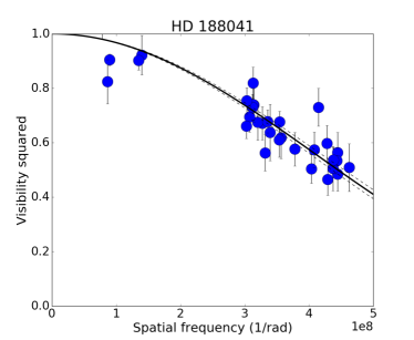
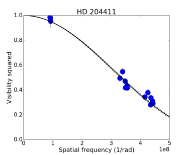
Figure 10: Squared visibility versus spatial frequency for HD 188041 (left panel) and for HD 204411 (right panel). Solid lines represent the best uniform-disk models provided by LITpro.

We used the model fitting tool LITpro to determine the uniform-disk angular diameter of our targets, and the Claret tables (Claret & Bloemen, 2011) to determine the limb-darkened angular diameters using a linear limb-darkening law in the R band. For HD 188041, we obtained an angular diameter of $\theta_{UD}$ = 0.238(5) mas, a limb-darkened angular diameter of $\theta_{UD}$ = 0.246(5) mas considering an effective temperature ranging from 8750 to 9250 K and a surface gravity ranging from 4 to 4.5. We used parallax values from GAIA DR2 release (Gaia Collaboration et al., 2018) with the error estimates as described in Section 4.2. Assuming a parallax of 11.72(11), we deduced a radius of $R$ = 2.26(5) $R_{\odot}$ for HD 188041.

For HD 204411, we obtained an angular diameter of $\theta_{UD}$ = 0.316(4) mas, a limb-darkened angular diameter of $\theta_{UD}$ = 0.328(4) mas considering an effective temperature ranging from 8250 to 8750 K and a surface gravity ranging from 4 to 4.5. Assuming a parallax of 8.33(12), we deduced a radius of $R$ = 4.23(8) $R_{\odot}$ for HD 204411.

The measured stellar radii allow us to derive effective temperatures from the bolometric flux using Stefan-Boltzmann law. The total flux for both stars was derived using photometric and spectrophotometric observations calibrated in absolute units. Photometric data were extracted from TD1 (Thompson et al., 1978), IUE archive, GAIA DR2 (Gaia Collaboration et al., 2018), 2MASS (Cutri et al., 2003), WISE (Cutri & et al., 2014) catalogues, while UV spectra and optical spectrophotometry were taken from IUE archive, from Adelman et al. (1989) and Breger (1976) catalogues. For HD 204411 we also plotted México observations described in Section 4.1 Fig. 11 shows the observed flux distribution for HD 188041 and HD 204411. Flux integration was performed using the spline interpolation along the observed data points. The dashed line represents the resulting SED employed for integration. UV zero point was taken at 912 Å. We obtained the bolometric fluxes $F=1.410\times 10^{-7}erg/cm^{2}/s$ (with TD1) and $F=1.364\times 10^{-7}erg/cm^{2}/s$ (with IUE) for HD 188041. In case of HD 204411 with different optical spectra/spectrophotometry we obtained $F=1.915\times 10^{-7}erg/cm^{2}/s$ (Adelman/Breger) and $F=2.000\times 10^{-7}erg/cm^{2}/s$ (OANSPM-1) Employing interferometric radii and assuming 10% uncertainty in flux determination we deduced effective temperatures of our stars to be 9060/8990(250) K (HD 188041) and 8560/8650(230) K (HD 204411). If we employ the radii derived by means of spectroscopy, the corresponding temperatures are 8880/8810 and 8360/8460 K, which agrees well with the spectroscopic determinations and validates our flux integration procedure and the adopted effective temperature uncertainty.

We also calculated bolometric flux $F=8.067\times 10^{-8}erg/cm^{2}/s$ for HD 111133 and estimated an effective temperature as 9590(250) K using spectroscopic radius. Again, the effective temperature derived from integrated flux agrees within the error with 9770(200) derived from self-consistent spectroscopic analysis.

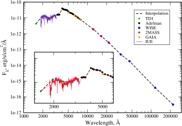
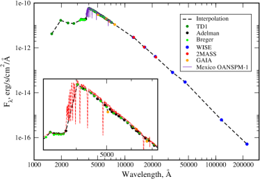
Figure 11: Observed flux distribution of HD 188041 (left panel) and HD 204411(right column). Interpolation curves are shown by dashed lines. Insets show parts of flux distributions with different overlapping observations.

6 Position of Ap stars on the HR diagram

Table 5 lists Ap stars with the fundamental parameters derived from the detailed self-consistent spectroscopic analysis taking into account abundance anomalies and stratification of the most important elements. We also added four more stars, HD 8441, HD 133792, HD 40312, and HD 112185 for which fundamental parameters were derived from detailed but not fully self-consistent spectroscopic analysis (Titarenko et al., 2012; Kochukhov et al., 2006, 2019). These stars are marked by italic font in Table 5. Note that the luminosities of the first two stars were recalculated based on the parallaxes from DR2 catalogue (3.44(10) and 5.49(5) mas). The values of the surface magnetic fields for most stars are taken from Ryabchikova et al. (2008) and references therein. For HD 40312 and HD 11218 the magnetic fields $\langle B_{\rm s}\rangle$  are taken from Table 4 of Kochukhov et al. (2019). No estimates of the $\langle B_{\rm s}\rangle$  in HD 8441 and HD 103498 are available, but according to Aurière et al. (2007) their longitudinal fields vary between -200 and 200 G. Assuming a commonly found in other stars poloidal dipole-dominant configuration, we find that most probably the surface magnetic field in these stars does not exceed 1 kG. The last four columns contain fundamental stellar parameters derived by interferometry together with the corresponding references.

Table 5: Fundamental parameters of Ap stars.

HD	Spectroscopy						Interferometry
	$T_{\rm eff}$	log ${g}$	$R/R_{\odot}$	$\log(L/L_{\odot})$	$\langle B_{\rm s}\rangle$,kG	Reference	$R/R_{\odot}$	$T_{\rm eff}$	$\log(L/L_{\odot})$	Reference
8441	9130(100)	3.45(17)		2.21(12)		Titarenko et al. (2012)
24712	7250(100)	4.10(15)	1.77(04)	0.89(07)	2.3	Shulyak et al. (2009)	1.77(06)	7235(280)	0.89(07)	Perraut et al. (2016)
40312	10400(100)	3.6(1)	4.64(17)	2.35(06)	0.4	Kochukhov et al. (2019)
101065	6400(200)	4.20(20)	1.98(03)	0.77(06)	2.3	Shulyak et al. (2010a)
103498	9500(150)	3.60(10)	4.39(75)	2.15(16)		Pandey et al. (2011)
1111331	9875(200)	3.40(20)	3.44(07)	2.00(04)	4.0	Current work
1111332	9875(200)	3.40(20)	2.92(44)	1.84(17)	4.0	Current work
112185	9200(200)	3.6(1)	4.08(14)	2.03(08)	0.1	Kochukhov et al. (2019)
128898	7500(130)	4.10(15)	1.94(01)	1.03(03)	2.0	Kochukhov et al. (2009)	1.97(07)	7420(170)	1.02(02)	Bruntt et al. (2008)
133792	9400(200)	3.7(1)	3.9(5)	2.02(10)	1.1	Kochukhov et al. (2006)
137909	8100(150)	4.00(15)	2.47(07)	1.37(08)	5.4	Shulyak et al. (2013)	2.63(09)	8160(200)	1.44(03)	Bruntt et al. (2010)
137949	7400(150)	4.00(15)	2.13(13)	1.09(15)	5.0	Shulyak et al. (2013)
176232	7550(050)	3.80(10)	2.46(06)	1.29(04)	1.5	Nesvacil et al. (2013)	2.32(09)	7800(170)	1.26(02)	Perraut et al. (2013)
188041	8770(150)	4.20(10)	2.39(05)	1.48(03)	3.6	Current work	2.26(05)	9060(250)	1.49(04)	Current work
201601	7550(150)	4.00(10)	2.07(05)	1.10(07)	4.0	Shulyak et al. (2013)	2.20(12)	7364(250)	1.11(05)	Perraut et al. (2011)
204411	8300(150)	3.60(10)	4.42(07)	1.92(04)	$\leq$0.8	Current work	4.23(08)	8560(230)	1.96(04)	Current work
Fundamental parameters derived by using original Hipparcos parallax1 and by GAIA DR22.

Comparison of the stellar radii derived by means of spectroscopy and interferometry (see Fig. 12) shows a reasonable agreement. Spectroscopic radii are larger by 7 % on average, which is well within 2$\sigma$ of the interferometric measurements. It means that spectroscopically derived radii will provide us with rather accurate estimates of this fundamental parameter for fainter Ap stars where interferometric observations are not yet possible.

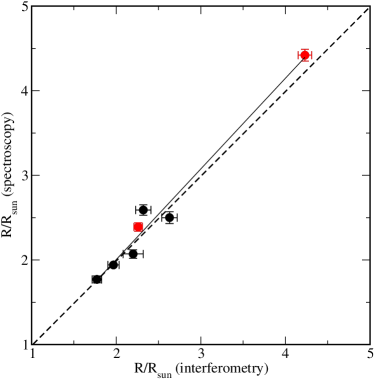
Figure 12: Comparison between stellar radii derived by means of spectroscopy and photometry. Data from the present work is shown by filled red circles. Solid and dashed lines indicate regression line and line of equal values.

Figure  13 shows the position of stars from Table 5 on the H-R diagram. Evolutionary tracks for the standard chemical composition models are taken from Girardi et al. (2000). Filled and open circles represent star’s position based on spectroscopic and interferometric data, respectively. The position of HD 111133 with the luminosity, calculated using the effective temperature and radius based on parallax value from the original Hipparcos catalogue is shown by filled green square.

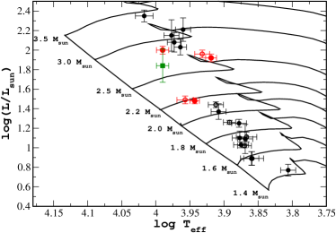
Figure 13: Ap stars on HR-diagram. Position of HD 111133, HD 188041, and HD 204411 from this work are shown by filled red circles (spectroscopy) and by open red circles (interferometry). Position of other stars are indicated by black filled circles (spectroscopy) and by open black circles (interferometry). Position of HD 111133 based on original Hipparcos parallax is marked by filled green square.

Although the number of objects shown in Fig.  13 is not enough for robust statistical analysis, some preliminary conclusions may be pointed out already now. Our sample of stars is clearly divided in two groups. About half of stars are located in the middle part of MS, which agrees well with the results of evolutionary study of Ap stars by Kochukhov & Bagnulo (2006). These stars possess moderately large magnetic fields and large REE overabundances. Group of stars with small magnetic fields (HD 8441, HD 40312, HD 103498, HD 112185 HD 133792, HD 204411) are close to finish their MS lives. Some of these stars also have minimal anomalies of the rare earth elements. Our results on field Ap stars are in line with the results of other evolutionary studies in Ap stars. They confirm the conclusion that the magnetic field strength decreases with age (Kochukhov & Bagnulo, 2006). They also support the conclusion drawn on the basis of an analysis of secular abundance variations in the atmospheres of Ap stars belonging to clusters of different ages that the REE anomaly weakens with time (Bailey et al., 2014). The only exception is HD 111133 which possess rather strong magnetic field but is located close to the group of evolved stars. As follows from Section 4.2.2 SED fit for this star is not as good as for other stars, in particular, in UV region. We also note the large parallax difference in Hipparcos and GAIA catalogues. The use of parallax from the original Hipparcos catalogue gives better result because it brings HD 111133 closer to group of stars with strong magnetic field, just as expected. It will be important to perform interferometric measurements for this star to pin down its position on H-R diagram. In any case, we need to analyse more objects with the reliably defined fundamental parameters in order to constrain evolution history of Ap stars.

7 Conclusion

In this work we carried out a detailed atmospheric analysis of three Ap stars employing high-resolution spectroscopy and (spectro)-photometry calibrated to flux units. For two of them, HD 188041 and HD 204411, we additionally obtained interferometric estimates of their angular diameters that allowed us to derive model-independent stellar radii. For HD 204411 we also analized medium resolution spectroscopic observations obtained with the Boller & Chivens long-slit spectrograph mounted at the $2.1$ m telescope of the Observatorio Astronómico Nacional at San Pedro Mártir, Baja California, México (OAN SPM). The results of our study are summarized as follows:

• We find a very good agreement between effective temperatures and radii derived by means of spectroscopy (employing model atmospheres) and interferometry (employing observed SED and radii derived from stellar angular diameters and parallaxes). It means that spectroscopically derived radii will provide us with rather accurate estimates of fundamental parameters for fainter Ap stars for which interferometric observations are not yet possible.

• Our empirical abundance stratification analysis is in a good agreement with the predictions of modern diffusion models, with the exception of Ca deficiency in the atmosphere of HD 111133. This needs additional investigation.

• Our results are consistent with the conclusion drawn in previous studies that the strength of the magnetic field and abundance anomalies weaken as stars age.

• For HD 118041 and HD 204411 we improved analysis of atmospheric abundances by including accurate Zeeman splitting in the equivalent width calculation.

• Spectroscopic observations obtained with Boller & Chivens spectrograph (OAN SPM, México) and their calibration agree well with similar data sets. However, the poor instrument performance in UV region around Balmer jump limits our ability to constrain accurate surface gravity and alternative observations should be used instead.

References

- Adelman et al. (1989) Adelman S. J., Pyper D. M., Shore S. N., White R. E., Warren Jr. W. H., 1989, A&AS, 81, 221
- Amôres & Lépine (2005) Amôres E. B., Lépine J. R. D., 2005, AJ, 130, 659
- Asplund et al. (2009) Asplund M., Grevesse N., Sauval A. J., Scott P., 2009, ARA&A, 47, 481
- Aurière et al. (2007) Aurière M., et al., 2007, A&A, 475, 1053
- Babel (1992) Babel J., 1992, A&A, 258, 449
- Bailey et al. (2014) Bailey J. D., Landstreet J. D., Bagnulo S., 2014, A&A, 561, A147
- Blackwell-Whitehead et al. (2005) Blackwell-Whitehead R. J., Pickering J. C., Pearse O., Nave G., 2005, ApJS, 157, 402
- Bonneau et al. (2006) Bonneau D., et al., 2006, A&A, 456, 789
- Bourges et al. (2017) Bourges L., Mella G., Lafrasse S., Duvert G., Chelli A., Le Bouquin J.-B., Delfosse X., Chesneau O., 2017, VizieR Online Data Catalog, 2346
- Breger (1976) Breger M., 1976, ApJS, 32, 7
- Bruntt et al. (2008) Bruntt H., et al., 2008, MNRAS, 386, 2039
- Bruntt et al. (2010) Bruntt H., et al., 2010, A&A, 512, A55
- Claret & Bloemen (2011) Claret A., Bloemen S., 2011, VizieR Online Data Catalog, 352
- Cohen et al. (2003) Cohen M., Wheaton W. A., Megeath S. T., 2003, AJ, 126, 1090
- Cutri & et al. (2014) Cutri R. M., et al. 2014, VizieR Online Data Catalog, p. II/328
- Cutri et al. (2003) Cutri R. M., et al., 2003, VizieR Online Data Catalog, 2246
- ESA (1997) ESA ed. 1997, The HIPPARCOS and TYCHO catalogues. Astrometric and photometric star catalogues derived from the ESA HIPPARCOS Space Astrometry Mission ESA Special Publication Vol. 1200
- Fitzpatrick (1999) Fitzpatrick E. L., 1999, PASP, 111, 63
- Gaia Collaboration et al. (2016) Gaia Collaboration et al., 2016, A&A, 595, A1
- Gaia Collaboration et al. (2018) Gaia Collaboration et al., 2018, A&A, 616, A1
- Girardi et al. (2000) Girardi L., Bressan A., Bertelli G., Chiosi C., 2000, A&AS, 141, 371
- Gontcharov & Mosenkov (2018) Gontcharov G. A., Mosenkov A. V., 2018, VizieR Online Data Catalog, p. II/354
- Green et al. (2018) Green G. M., et al., 2018, MNRAS, 478, 651
- Grevesse et al. (2015) Grevesse N., Scott P., Asplund M., Sauval A. J., 2015, A&A, 573, A27
- Hayes & Latham (1975) Hayes D. S., Latham D. W., 1975, ApJ, 197, 593
- Holt et al. (1999) Holt R. A., Scholl T. J., Rosner S. D., 1999, MNRAS, 306, 107
- Khan & Shulyak (2007) Khan S. A., Shulyak D. V., 2007, A&A, 469, 1083
- Kochukhov (2007) Kochukhov O. P., 2007, in Romanyuk I. I., Kudryavtsev D. O., Neizvestnaya O. M., Shapoval V. M., eds, Physics of Magnetic Stars. pp 109–118 (arXiv:astro-ph/0701084)
- Kochukhov (2018) Kochukhov O., 2018, BinMag: Widget for comparing stellar observed with theoretical spectra, Astrophysics Source Code Library (ascl:1805.015)
- Kochukhov & Bagnulo (2006) Kochukhov O., Bagnulo S., 2006, A&A, 450, 763
- Kochukhov et al. (2006) Kochukhov O., Tsymbal V., Ryabchikova T., Makaganyk V., Bagnulo S., 2006, A&A, 460, 831
- Kochukhov et al. (2009) Kochukhov O., Shulyak D., Ryabchikova T., 2009, A&A, 499, 851
- Kochukhov et al. (2010) Kochukhov O., Makaganiuk V., Piskunov N., 2010, A&A, 524, A5
- Kochukhov et al. (2019) Kochukhov O., Shultz M., Neiner C., 2019, A&A, 621, A47
- Krtička et al. (2009) Krtička J., Mikulášek Z., Henry G. W., Zverko J., Žižovský J., Skalický J., Zvěřina P., 2009, A&A, 499, 567
- Krtička et al. (2012) Krtička J., Mikulášek Z., Lüftinger T., Shulyak D., Zverko J., Žižňovský J., Sokolov N. A., 2012, A&A, 537, A14
- Krtička et al. (2015) Krtička J., Mikulášek Z., Lüftinger T., Jagelka M., 2015, A&A, 576, A82
- Kupka et al. (1999) Kupka F., Piskunov N., Ryabchikova T. A., Stempels H. C., Weiss W. W., 1999, A&AS, 138, 119
- Lallement et al. (2018) Lallement R., et al., 2018, A&A, 616, A132
- Landi Degl’Innocenti (1975) Landi Degl’Innocenti E., 1975, A&A, 45, 269
- LeBlanc et al. (2009) LeBlanc F., Monin D., Hui-Bon-Hoa A., Hauschildt P. H., 2009, A&A, 495, 937
- Leblanc & Monin (2005) Leblanc F., Monin D., 2005, JRASC, 99, 139
- Maitzen (1976) Maitzen H. M., 1976, A&A, 51, 223
- Maitzen et al. (1998) Maitzen H. M., Pressberger R., Paunzen E., 1998, A&AS, 128, 573
- Michaud (1970) Michaud G., 1970, ApJ, 160, 641
- Molnar (1973) Molnar M. R., 1973, in BAAS. p. 325
- Mourard et al. (2009) Mourard D., et al., 2009, A&A, 508, 1073
- Nesvacil et al. (2013) Nesvacil N., Shulyak D., Ryabchikova T. A., Kochukhov O., Akberov A., Weiss W., 2013, A&A, 552, A28
- Netopil et al. (2008) Netopil M., Paunzen E., Maitzen H. M., North P., Hubrig S., 2008, A&A, 491, 545
- Pandey et al. (2011) Pandey C. P., Shulyak D. V., Ryabchikova T., Kochukhov O., 2011, MNRAS, 417, 444
- Perraut et al. (2011) Perraut K., et al., 2011, A&A, 526, A89
- Perraut et al. (2013) Perraut K., et al., 2013, A&A, 559, A21
- Perraut et al. (2016) Perraut K., Brandão I., Cunha M., Shulyak D., Mourard D., Nardetto N., ten Brummelaar T. A., 2016, A&A, 590, A117
- Pickering (1996) Pickering J. C., 1996, Astrophysical Journal Supplement Series, 107, 811
- Renson & Manfroid (2009) Renson P., Manfroid J., 2009, A&A, 498, 961
- Romanyuk & Kudryavtsev (2008) Romanyuk I. I., Kudryavtsev D. O., 2008, Astrophysical Bulletin, 63, 139
- Ryabchikova (1991) Ryabchikova T. A., 1991, in Michaud G., Tutukov A. V., eds, IAU Symposium Vol. 145, Evolution of Stars: the Photospheric Abundance Connection. p. 149
- Ryabchikova & Romanovskaya (2017) Ryabchikova T. A., Romanovskaya A. M., 2017, Astronomy Letters, 43, 252
- Ryabchikova et al. (2002) Ryabchikova T., Piskunov N., Kochukhov O., Tsymbal V., Mittermayer P., Weiss W. W., 2002, A&A, 384, 545
- Ryabchikova et al. (2003) Ryabchikova T., Wade G. A., LeBlanc F., 2003, in Piskunov N., Weiss W. W., Gray D. F., eds, IAU Symposium Vol. 210, Modelling of Stellar Atmospheres. p. 301
- Ryabchikova et al. (2004) Ryabchikova T., Nesvacil N., Weiss W. W., Kochukhov O., Stütz C., 2004, A&A, 423, 705
- Ryabchikova et al. (2005) Ryabchikova T., Leone F., Kochukhov O., 2005, A&A, 438, 973
- Ryabchikova et al. (2008) Ryabchikova T., Kochukhov O., Bagnulo S., 2008, A&A, 480, 811
- Ryabchikova et al. (2015) Ryabchikova T., Piskunov N., Kurucz R. L., Stempels H. C., Heiter U., Pakhomov Y., Barklem P. S., 2015, Phys. Scr, 90, 054005
- Scott et al. (2015a) Scott P., et al., 2015a, A&A, 573, A25
- Scott et al. (2015b) Scott P., Asplund M., Grevesse N., Bergemann M., Sauval A. J., 2015b, A&A, 573, A26
- Shulyak et al. (2004) Shulyak D., Tsymbal V., Ryabchikova T., Stütz C., Weiss W. W., 2004, A&A, 428, 993
- Shulyak et al. (2009) Shulyak D., Ryabchikova T., Mashonkina L., Kochukhov O., 2009, A&A, 499, 879
- Shulyak et al. (2010a) Shulyak D., Ryabchikova T., Kildiyarova R., Kochukhov O., 2010a, A&A, 520, A88
- Shulyak et al. (2010b) Shulyak D., Krtička J., Mikulášek Z., Kochukhov O., Lüftinger T., 2010b, A&A, 524, A66
- Shulyak et al. (2013) Shulyak D., Ryabchikova T., Kochukhov O., 2013, A&A, 551, A14
- Thompson et al. (1978) Thompson G. I., Nandy K., Jamar C., Monfils A., Houziaux L., Carnochan D. J., Wilson R., 1978, Catalogue of stellar ultraviolet fluxes. A compilation of absolute stellar fluxes measured by the Sky Survey Telescope (S2/68) aboard the ESRO satellite TD-1
- Titarenko et al. (2012) Titarenko A. R., Semenko E. A., Ryabchikova T. A., 2012, Astronomy Letters, 38, 721
- Villemoes et al. (1993) Villemoes P., Arnesen A., Heijkenskjold F., Wannstrom A., 1993, Journal of Physics B Atomic Molecular Physics, 26, 4289
- ten Brummelaar et al. (2005) ten Brummelaar T. A., et al., 2005, ApJ, 628, 453
- van Leeuwen (2007) van Leeuwen F., 2007, A&A, 474, 653