ASR Model Compression Using AutoML

Automatic Speech Recognition Model Compression Using Low-Rank Matrix Factorization through Reinforcement Learning

ASR Model Compression Using SVD through Reinforcement Learning

ASR Model Compression Using SVD through AutoML

ASR Model Compression Using SVD Through Reinforcement Learning

Shrinking MoChA: Automatic ASR
Model Compression Using Reinforcement Learning

Shrinking ASR:
Model Compression Using Reinforcement Learning

Shrinking End-to-End ASR:
Model Compression Using Reinforcement Learning

ShrinkML: End-to-End ASR Model
Compression Using Reinforcement Learning

Abstract

End-to-end automatic speech recognition (ASR) models are increasingly large and complex to achieve the best possible accuracy. In this paper, we build an AutoML system that uses reinforcement learning (RL) to optimize the per-layer compression ratios when applied to a state-of-the-art attention based end-to-end ASR model composed of several LSTM layers. We use singular value decomposition (SVD) low-rank matrix factorization as the compression method. For our RL-based AutoML system, we focus on practical considerations such as the choice of the reward/punishment functions, the formation of an effective search space, and the creation of a representative but small data set for quick evaluation between search steps. Finally, we present accuracy results on LibriSpeech of the model compressed by our AutoML system, and we compare it to manually-compressed models. Our results show that in the absence of retraining our RL-based search is an effective and practical method to compress a production-grade ASR system. When retraining is possible, we show that our AutoML system can select better highly-compressed seed models compared to manually hand-crafted rank selection, thus allowing for more compression than previously possible.

1 Introduction

End-to-end automatic speech recognition (ASR) models have outperformed traditional ASR systems. In particular, models with attention mechanism [1] have produced state-of-the-art results in speech recognition and translation application domains [2, 3, 4]. These models improve upon traditional systems, partially because they include acoustic models, language models and pronunciation dictionary jointly learned together. Furthermore, models with character/subword output units are especially useful in low latency deployments such as mobile phones and can produce good results with a beam-search decoding mechanism [5].

One challenge when encompassing all components of ASR into a single model is the need for larger model capacity and thereby deeper neural networks with several recurrent layers. This makes it harder to achieve real-time inference, especially with on-device deployments. One approach to reduce model size is to apply model compression techniques [6]. This is often done manually and may include many trial-and-error experiments until a reasonable compression scheme is found. However, more recently, automated search-based techniques have been employed to optimize the compression of deep neural networks [7]. More specifically, AutoML has been used to select the per-layer compression ratios to optimize a model globally.

In this paper, we use reinforcement learning to select the per-layer compression ratios based on matrix approximation using singular value decomposition (SVD) [8]. We base our work on a recently proposed end-to-end ASR model with attention mechanism [9, 10] that has obtained state-of-the-art results on LibriSpeech. We focus on practical aspects when designing the AutoML compression system in the specific context of ASR models. We show experimentally that our approach is superior to manual model compression for both modest and aggressive compression targets, in the absence or presence of retraining. In the following sections, we outline the ASR model and present insights into compressibility of layers in such encoder-attention-decoder models, describe the AutoML framework and present a data subsampling technique to speed up the search process, and finally delve into experimental results that prove the efficacy of our system, corroborated by on-device measurements on a mobile phone.

2 ASR Model Compression

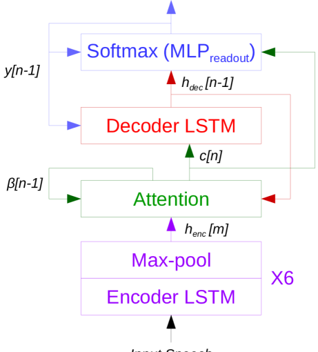
Figure 1: End-to-end ASR model architecture.

2.1 ASR Model

We use an end-to-end attention based ASR model [11, 12] with an architecture similar to the one proposed in [10] as depicted in Fig. 1. The main differences in our model are the use of 1) unidirectional LSTMs in place of bidirectional LSTMs and 2) monotonic chunk-wise attention [13]. These changes were made to allow the model to decode speech in streaming mode, which is required for mobile applications. As a result, the model also has a higher baseline word error rate (WER) as compared to the results published in [10]. The unit size for all LSTM layers in the network is 1024 and the output layer comprises 10000 sized byte-pair encoded sub-word units [14, 15]. The model was trained on LibriSpeech training set [16] with MFCC front-end using Tensorflow [17] and the RETURNN framework [18]. A time reduction factor of 8 was used via the maxpool layers interleaved between the first four encoder LSTM layers. In this work we have not used a separate language model for further reduction of WER.

2.2 Low-Rank Matrix Approximation

Our primary target is to build a generic reinforcement learning (RL) based AutoML system that automatically optimizes the per-layer compression ratios for ASR models. We decide to choose low-rank matrix factorization, and specifically, singular-value decomposition (SVD) to compress the weight matrices, since it has proven to be an effective method for compressing similar models [19, 20, 21, 22, 23, 24]. However, we design our system such that it is generalizable to different compression methodologies. We refer the reader to prior work for further reading on SVD, but a summary is given below. We factorize a matrix $M$ into three matrices $U$, $\Sigma$ and $V$:

$$M=U\Sigma V^{T}$$ (1)

where $\Sigma$ is a diagonal matrix which consists of the singular values (typically in descending order of magnitude) that uniquely identify $M$. We compress $M$ by removing the lower-magnitude values in $\Sigma$ – we refer to the number of remaining element as a factorization rank and denote it with $k$. We select $k$ in such a way that it preserves a given energy, where energy refers to the normalized summation of the remaining singular values. We then remove corresponding columns from matrices $U$ and $V$, creating a set of three new matrices $U^{\prime}$, $\Sigma^{\prime}$ and $V^{\prime}$ which approximate original matrix $M$. Finally, we combine $\Sigma^{\prime}$ with $V^{\prime}$ so that we can replace $M$ according to the following equation:

$$M\approx U^{\prime}V^{*}=U^{\prime}\Sigma^{\prime}{V^{\prime}}^{T}$$ (2)

If $M$ is an $m\times n$ matrix, then $U^{\prime}$ and $V^{*}$ have dimensions $m\times k$ and $k\times n$ respectively, and we get a theoretical speedup and model size reduction:

$$Speedup=\frac{m\times n}{k\times(m+n)}$$ (3)

3 AutoML for SVD Rank Selection

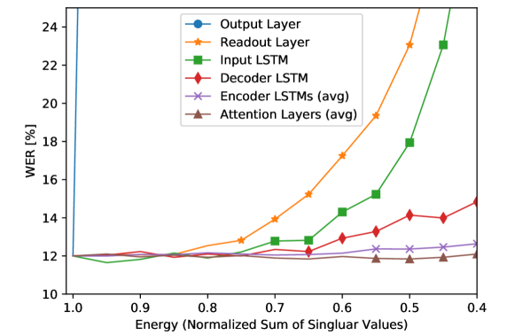
Figure 2: Single-layer compression gives an indication of the relative sensitivity of the model to each layer, and instructs the acceptable compression ranges for our RL-based search.

Fig. 2 plots the WER degradation when each of the layers are factorized separately – as shown, the model accuracy is much more sensitive to changes in the input and output layers, but less so to intermediate encoder LSTM cells, attention and decoder layers. Selecting the ranks per layer for the 18 matrices in the model is a hard problem because of the large number of combinations. For instance, if we discretize compression range for each layer to 5 rank options, we have $5^{18}=3.8\times 10^{12}$ possible factorizations. We use reinforcement learning to navigate that search space and find the best compression schemes.

3.1 AutoML System

We use an RL-based system similar to the one proposed by [25] after slightly adapting it for the model compression task. More specifically, in our case an agent is responsible for deciding the factorization scheme which would: a) guarantee a predefined speedup, and b) minimize WER of the factorized model. The scheme in this context is a series of decisions, with each decision representing a compression ratio for an individual layer. Both the list of layers and the set of discrete compression levels per layer are provided a priori to the search. We call the set of all possible factorization schemes a search space and the set of all parameters which modify it hyperparameters of the search space. More formally, our search space can be defined as a 2-dimensional matrix: $S\in\mathbb{Z}^{l\times d}$, where $S_{i,j}$ represents a rank $k$ to use when factorizing the $i$-th layer according to the $j$-th option. From this search space, the agent selects a factorization scheme $s\in\mathbb{Z}^{l}$ by choosing one value from each row of matrix $S$. The selection is done by sampling $l$ probability distributions over $d$ options which are produced by a trainable policy $\pi(\theta)$.

In our system, this policy is modeled with a single LSTM layer with 100 input units and 100 hidden units which takes a sequence of $l$ inputs (one for each layer) – each element of output sequence is then passed to its individual fully-connected layer with $d$ units, to match its length with the number of available decisions, followed by softmax. The final output is $D\in\mathbb{R}^{l\times d}$ where each vector $D_{i}\in\mathbb{R}^{d}$ represents probability distribution of selecting different factorization options for the $i$-th layer. We reward the agent depending on the WER of the model when compressed according to the proposed scheme, and use policy gradient to update $\theta$.

3.2 AutoML System Tuning for Compression

Input: Policy weights $\theta$, set of explored points $\mathbb{W}$, search space $S$, target speedup $a_{t}$

Output: Updated $\theta$ and $\mathbb{W}$

1 $D\leftarrow\pi(\theta)$

2 $\hskip 2.84544pts\leftarrow\mymathbb{0}_{l}$

3 $\hskip 2.84544ptp\leftarrow\mymathbb{0}_{l}$

4 for $i$ $\leftarrow$ $0$ to $l$ do

5       $j\sim D_{i}$

6       $s_{i}$ $\leftarrow$ $S_{i,j}$

7       $p_{i}$ $\leftarrow$ $D_{i,j}$

8 end for

9$a$ $\leftarrow$ estimate speedup achievable by $s$

10 if $a<a_{t}$ then

11       $\Delta_{a}\leftarrow a_{t}-a$

12       $r\leftarrow\mathcal{R}_{v}(\Delta_{a})$

13      

14else

15       $w$ $\leftarrow$ compress model according to $s$ and evaluate WER on a proxy dataset

16       $r$ $\leftarrow$ $\mathcal{R}(w)$

17       $\mathbb{W}$ $\leftarrow$ $\mathbb{W}\cup\{(s,w)\}$

18      

19 end if

20$\theta$ $\leftarrow$ update $\theta$ using $\nabla(-\log(\prod_{i=0}^{l}p_{i})r)$

21

Algorithm 1 A single step of the proposed search.

One of the main challenges for many AutoML systems is reducing the time required to produce useful results. RL-based search is slow because evaluation of a proposed action (in our case, running evaluation on a validation set) takes significantly more time than proposing a new action. In this work we address this problem and propose a number of techniques which we have successfully used to significantly reduce evaluation time. This way, we speed up the search, while still providing representative feedback to the RL agent.

To quickly reject unprofitable points, we estimate speedup of a proposed scheme ($a$) and compare it to the predefined target ($a_{t}$), as shown in Algorithm 1. If it falls below the threshold, we punish the agent using a dedicated reward function $\mathcal{R}_{v}$, otherwise the scheme is accepted for full evaluation and we reward the controller according to returned WER using reward function $\mathcal{R}$. We observed that combined usage of the two reward functions makes the search converge to a certain area of the speedup-WER plane – as presented in Fig. 4 – with $\mathcal{R}$ pushing points towards smaller WER and $\mathcal{R}_{v}$ pushing above $a_{t}$. However, both functions need to be tuned relative to each other, as well as independently, to obtain good results. In our work we empirically found that when targeting conservative $a_{t}$ values relative differences in WER between the original model ($w_{b}$) and its compressed versions ($w$) might be too small to make the agent discriminate between good models with similar WERs. Therefore, we decided to use exponential function to add additional emphasis to the difference:

$$\mathcal{R}(w)=-\exp(w-w_{b})$$ (4)

However, the range of this function is too big when targeting high speedups $a_{t}$, because the WER range is much larger, so we used a slightly modified version for such aggressive searches:

$$\mathcal{R}(w)=-\exp(\sqrt{\frac{w}{w_{b}}})$$ (5)

For both aggressive and conservative compression we observed that a simple linear function works well for $\mathcal{R}_{v}$, with parameters $-100$ and $-10$ tuned to make its values visibly worse than $\mathcal{R}$, even when $\Delta_{a}\rightarrow 0$.

$$\mathcal{R}_{v}(\Delta_{a})=-100\Delta_{a}-10$$ (6)

3.3 Small Dataset Creation

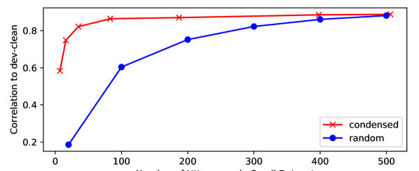
Figure 3: Correlation of small datasets with the full-size validation sets. Our “condense” algorithm is more successful in creating smaller representative datasets for use with AutoML.

LibriSpeech validation sets consist of 5567 utterances split among dev-clean and dev-other. Using the validation sets to evaluate WER for each model proposed by AutoML was too slow and led us to investigate if a representative subset could be found. First, we tried randomly selecting utterances from the validation sets. However, we observed experimentally that this did not work well with small random sets – if we minimize WER on the random set, this does not always translate into a lower WER on the full-size validation or test sets. Instead, we used our “condense” algorithm in Listing 1 to select the utterances that were most representative of the validation sets.

⬇

1#wer_avg_all is a list containing WER on whole dev set w.r.t. cohort models

2for utterance in validation_sets:

3 wer_utt= []

4 for c_model in cohort_models:

5 wer_utt.append(

6 compute_wer(utterance,c_model))

7 correl[utterance] =

8 correlation(wer_utt, wer_avg_all)

9

10#filter utterances < min_correl and min_length

11for utterance in validation_sets:

12 if correl[utterance] > correl_min:

13 new_set.append(sample)

Listing 1: Heuristic to find “condensed” datasets in Fig. 3.

As Listing 1 shows, we find the WER per utterance from different cohort models. These models are simple variations of our baseline model presented in Section 2.1 – we use 8 cohort models trained with different number of layers, layer sizes in the encoder, and few variations of SVD-based compression schemes. We compile the WERs of each utterance when decoded with each of these models, and correlate that to the WERs of the entire validation set with the same models. We then choose the utterances that correlate highly in WER with the entire set across all the cohort models. As Fig. 3 shows, our “condensed” datasets correlate much better than “random” sets, especially with very small dataset sizes. With ${correl}\_{min}=0.95$ we created an 83-sample dataset for use with AutoML – this is 67$\times$ smaller than the validation sets but was highly-correlated with the full set as Fig. 3 shows. We used it as a drop-in replacement for AutoML thus making the whole system $>$10$\times$ faster overall.

4 Results

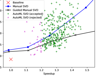
(a) Steps 0 to 300.

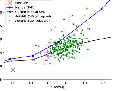
(b) Steps 600 to 900.

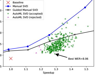
(c) Steps 1600 to 1900.

Figure 4: Comparison of the RL search with naïve manual SVD compression (all layers with equal energy), and “guided” manual SVD (excludes sensitive layers identified in Fig. 2). As the search progresses, results that outperform manual compression are explored.

We use AutoML for two experiments. First, we want to find a modestly-compressed model with minimal WER loss in the absence of retraining. We believe that full training data is not always available, especially in systems where all of the training data is not in one place [26], or when app developers are using pretrained models and do not have access to training sets. Second, we use AutoML to find the best aggressively-compressed seed model for retraining. In this case we maximize compression, and rely on retraining to recover the accuracy.

4.1 Compression without Retraining

We launched two searches, slow and fast, both targeting speedup $a_{t}=1.2$, and using Equations 4 and 6. The slow search evaluated models on the entire dev-clean dataset and selected compression ratios for each layer from the same range. The fast search used the condensed dataset described in the previous section and had per-layer compression ranges adjusted according to the information from Fig. 2. To extract the best model, for each search independently we gathered all explored configurations and selected top-5 (as evaluated by the search) which were then evaluated on the “test” datasets from LibriSpeech (test-clean and test-other). The best model reported here is the best of the 5 on test-clean. As shown in Table 1, the fast search was able to find an equally-good compression scheme much faster. Both searches were also able to find better compression schemes than the hand-crafted manual ones as highlighted in Fig 4.

Table 1: Evaluation of the best models found by both searches. Steps mean at what step during the search a model was found.

	AutoML		Manual	Baseline
	Slow	Fast	Guided
test-clean	8.35	8.34	8.67	8.29
test-other	21.61	21.33	22.04	21.13
step	1626	2363	NA
GPU hours	635	74

4.2 Aggressive Compression With Retraining

Previous work has repeatedly proven that SVD-based compression is very effective in attaining speedup while maintaining model accuracy when retraining is available [19, 21, 23]. We use our “guided manual” method of compression to test the limits of compression with retraining. We train for 50 epochs over LibriSpeech with an epoch split of 20 – this means we go through the training data 2.5 times. As Fig. 5 shows, we achieved up to ~3$\times$ compression without degrading WER on test-clean. Can we push this any further using our AutoML system? To answer this question, we set our speedup threshold to 3.7$\times$ and launched our fast AutoML search for only a few hours, we then used the best-found model as the seed model for retraining and the results are shown in Fig. 5. The model found by AutoML achieved 3.75$\times$ speedup and had approximately half the WER before retraining when compared to the manually-compressed model at the same speedup. After retraining, we were able to recover almost full accuracy, as shown in Fig. 5, therefore, we believe this is an effective systematic method to selecting highly-compressed models for retraining. After 8-bit quantization, the model size is compressed to 24 MB from the 32-bit compressed model size of 72 MB.

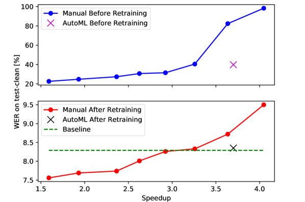
Figure 5: WER before/after retraining for “guided manual” and AutoML compressed models.

4.3 On-Device Measurements and Considerations

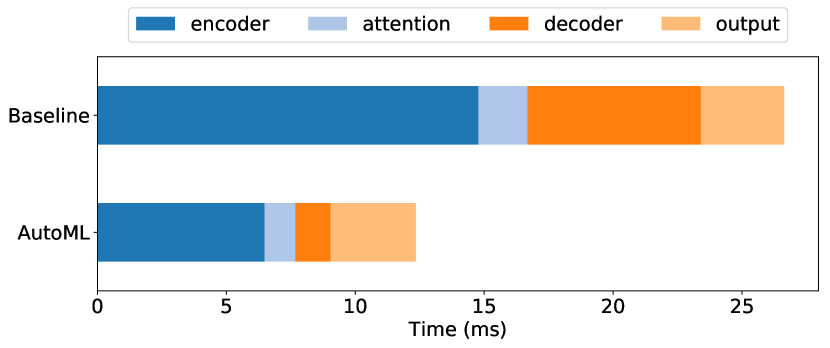
Figure 6: Runtime on Qualcomm Snapdragon 845 chipset.

So far, we have been using Equation 3 as a proxy for speedup, however, we measured the actual on-device runtime of our retrained model from Section 4.2 to validate our estimate. We evaluate on a Qualcomm Snapdragon 845 development board, using TFLite [27] on CPU. As depicted in Fig. 6, we acquire a significant speedup of 2.16$\times$ with our SVD-based compressed model over the baseline – especially in the encoder and decoder parts of the network. However, this is much lower than the estimated 3.74$\times$ shown in Fig 5. We shall investigate this discrepancy in future work but mention this here as a note that theoretical and measured speedups often vary greatly.

5 Conclusion

In this work, we presented an AutoML framework to push the boundaries of SVD-based ASR model compression beyond what is possible manually. We improved upon the WER attainable by manual compression when retraining is not possible. Even when we could retrain, we have shown that AutoML can improve the compression ratio, and therefore speedup, of our ASR model without any loss of accuracy. In the future we aim to use AutoML to optimize and mix different compression techniques, and we hope to make the estimated speedup/accuracy in such a system more faithful to the actual results.

6 Acknowledgements

MoChA within the experimental framework was implemented by Dr. Chanwoo Kim and his team in Samsung research. We would like to thank them for their support and feedback.

References

- [1] D. Bahdanau, K. Cho, and Y. Bengio, “Neural machine translation by jointly learning to align and translate,” CoRR, vol. abs/1409.0473, 2015.
- [2] W. Chan, N. Jaitly, Q. V. Le, and O. Vinyals, “Listen, attend and spell: A neural network for large vocabulary conversational speech recognition,” 2016 IEEE International Conference on Acoustics, Speech and Signal Processing (ICASSP), pp. 4960–4964, 2016.
- [3] J. Chorowski, D. Bahdanau, K. Cho, and Y. Bengio, “End-to-end continuous speech recognition using attention-based recurrent nn: First results,” CoRR, vol. abs/1412.1602, 2014.
- [4] T. Luong, H. Q. Pham, and C. D. Manning, “Effective approaches to attention-based neural machine translation,” in EMNLP, 2015.
- [5] Y. He, T. N. Sainath, R. Prabhavalkar, I. McGraw, R. Alvarez, D. Zhao, D. Rybach, A. Kannan, Y. Wu, R. Pang, Q. Liang, D. Bhatia, Y. Shangguan, B. Li, G. Pundak, K. C. Sim, T. Bagby, S. Chang, K. Rao, and A. Gruenstein, “Streaming end-to-end speech recognition for mobile devices,” CoRR, vol. abs/1811.06621, 2018. [Online]. Available: http://arxiv.org/abs/1811.06621
- [6] R. Pang, T. Sainath, R. Prabhavalkar, S. Gupta, Y. Wu, S. Zhang, and C.-C. Chiu, “Compression of end-to-end models,” in Interspeech 2018. ISCA, pp. 27–31.
- [7] Y. He, J. Lin, Z. Liu, H. Wang, L.-J. Li, and S. Han, “Amc: Automl for model compression and acceleration on mobile devices,” in The European Conference on Computer Vision (ECCV), September 2018.
- [8] S. Bhattacharya and N. D. Lane, “Sparsification and separation of deep learning layers for constrained resource inference on wearables,” in Proceedings of the 14th ACM Conference on Embedded Network Sensor Systems CD-ROM, ser. SenSys ’16. New York, NY, USA: ACM, 2016, pp. 176–189. [Online]. Available: http://doi.acm.org/10.1145/2994551.2994564
- [9] A. Zeyer, A. Merboldt, R. Schlüter, and H. Ney, “A comprehensive analysis on attention models,” in NIPS, 2018.
- [10] A. Zeyer, K. Irie, R. Schlüter, and H. Ney, “Improved training of end-to-end attention models for speech recognition,” in Interspeech, 2018, pp. 7–11.
- [11] C. Kim, S. Kim, K. Kim, M. Kumar, J. Kim, K. Lee, C. Han, A. Garg, E. Kim, M. Shin, S. Singh, L. Heck, and D. Gowda, “End-to-end training of a large vocabulary end-to-end speech recognition system,” in ASRU, 2019.
- [12] K. Kim*, K. Lee*, D. Gowda, J. Park, S. Kim, E. S. Kim, Y.-Y. Lee, J. Yeo, D. Kim, S. Jung, J. Lee, M. Han, and C. Kim, “Attention based on-device streaming speech recognition with large speech corpus,” in ASRU, 2019.
- [13] C.-C. Chiu and C. Raffel, “Monotonic chunkwise attention,” in International Conference on Learning Representations, 2018.
- [14] R. Sennrich, B. Haddow, and A. Birch, “Neural machine translation of rare words with subword units,” in ACL, Berlin, Germany, Aug. 2016, pp. 1715–1725.
- [15] D. Gowda, A. Garg, K. Kim, M. Kumar, and C. Kim, “Multi-task multi-resolution char-to-bpe cross-attention decoder for end-to-end speech recognition,” in INTERSPEECH, 2019.
- [16] V. Panayotov, G. Chen, D. Povey, and S. Khudanpur, “Librispeech: An ASR corpus based on public domain audio books,” in ICASSP, 2015, pp. 5206–5210.
- [17] Tensorflow development team, “TensorFlow: Large-scale machine learning on heterogeneous systems,” 2015, software available from tensorflow.org. [Online]. Available: http://tensorflow.org/
- [18] A. Zeyer, T. Alkhouli, and H. Ney, “RETURNN as a generic flexible neural toolkit with application to translation and speech recognition,” in Proceedings of ACL, Melbourne, Australia, Jul. 2018, pp. 128–133.
- [19] J. Xue, J. Li, and Y. Gong, “Restructuring of deep neural network acoustic models with singular value decomposition,” in INTERSPEECH, 2013.
- [20] J. Xue, J. Li, D. Yu, M. Seltzer, and Y. Gong, “Singular value decomposition based low-footprint speaker adaptation and personalization for deep neural network,” in IEEE International Conference on Acoustics, Speech and Signal Processing (ICASSP), May 2014, pp. 6359–6363.
- [21] M. Sun, D. Snyder, Y. Gao, V. Nagaraja, M. Rodehorst, S. Panchapagesan, N. Strom, S. Matsoukas, and S. Vitaladevuni, “Compressed time delay neural network for small-footprint keyword spotting,” in Conference of the International Speech Communication Association (INTERSPEECH), August 2017, pp. 3607–3611.
- [22] G. Tucker, M. Wu, M. Sun, S. Panchapagesan, G. Fu, and S. Vitaladevuni, “Model compression applied to small-footprint keyword spotting,” pp. 1878–1882.
- [23] R. Prabhavalkar, O. Alsharif, A. Bruguier, and I. McGraw, “On the compression of recurrent neural networks with an application to LVCSR acoustic modeling for embedded speech recognition.” [Online]. Available: http://arxiv.org/abs/1603.08042
- [24] D. Povey, G. Cheng, Y. Wang, K. Li, H. Xu, M. Yarmohammadi, and S. Khudanpur, “Semi-orthogonal low-rank matrix factorization for deep neural networks,” in Interspeech 2018. ISCA, pp. 3743–3747.
- [25] B. Zoph and Q. V. Le, “Neural architecture search with reinforcement learning,” in International Conference on Learning Representation (ICLR), 2017.
- [26] J. Konečný, H. B. McMahan, F. X. Yu, P. Richtarik, A. T. Suresh, and D. Bacon, “Federated learning: Strategies for improving communication efficiency,” in NIPS Workshop on Private Multi-Party Machine Learning, 2016. [Online]. Available: https://arxiv.org/abs/1610.05492
- [27] “TensorFlow Lite,” 2019. [Online]. Available: http://tensorflow.org/lite