Expeditious computation of nonlinear optical properties of arbitrary order with native electronic interactions in the time domain

Abstract

We adapted a recently proposed framework to characterize the optical response of interacting electrons in solids in order to expedite its computation without compromise in accuracy at the microscopic level. Our formulation is based on reliable parameterizations of Hamiltonians and Coulomb interactions, which allows economy and flexibility in obtaining response functions. It is suited to computing the optical response to fields of arbitrary temporal shape and strength, to arbitrary order in the field, and natively accounts for excitonic effects. We demonstrate the approach by computing the frequency-dependent susceptibilities of MoS₂ and hexagonal BN monolayers up to the third-harmonic. Grounded on a generic non-equilibrium many-body perturbation theory, this framework allows extensions to handle generic interaction models or to describe electronic processes taking place at ultrafast time scales.

I Introduction

The nonlinear optical response of crystalline materials is a rich and attractive playground for optoelectronic applications Boyd (2008); Luppi and Véniard (2016). Traditionally, only a few select bulk crystals were considered of practical interest because nonlinearities tend to be weak effects Boyd (2008). But the recent advent and proliferation of countless two-dimensional (2D) materials have enormously broadened the range of platforms for studying nonlinear optical properties Wang et al. (2012); Xia et al. (2014); Luppi and Véniard (2016); Wang et al. (2018). Several classes of 2D crystals host a range of new electronic effects and functionalities, including nontrivial topological characteristics Xu et al. (2014); Schaibley et al. (2016) and enhanced electronic interactions, which arise from their strict two-dimensionality Cudazzo et al. (2011); Thygesen (2017); Kotov et al. (2012). One specific implication of enhanced interactions is that excitons become an essential element of the optical response of 2D semiconductors over extended frequency ranges Wang et al. (2018); Ridolfi et al. (2018). Moreover, excitons play a particularly critical role in high-order effects such as harmonic generation. For example, 2D transition metal dichalchogenide (TMD) semiconductors harbour bound excitons at energies practically resonant with lasers in standard use, thereby showing a consistently strong and easy-to-access nonlinear response Wang et al. (2018); Liu et al. (2016). For these reasons, the ability to theoretically understand and model these nonlinear characteristics is of very high current interest.

The strong optical response of 2D semiconductors also means they can more efficiently be driven out of equilibrium by optical excitation. This is of fundamental interest to probe and understand microscopic mechanisms underlying a number of proposed functionalities, including their valley and spin relaxation characteristics that are crucial for applications in valleytronics and spintronics, respectively Xu et al. (2014); Schaibley et al. (2016). Ultrafast spectroscopy experiments are a versatile and proven tool in this regard Huber et al. (2001); Kampfrath et al. (2013); Kim et al. (2014); Hao et al. (2016); Ye et al. (2017) which, in turn, demands realistic and accurate theoretical methods to model the microscopic transient response of electrons on fast timescales. Here, too, interactions are essential, not only to capture the correct excitations, but also the hot relaxation pathways at short timescales.

Unfortunately, handling interactions within accurate descriptions of the underlying electronic structure, such as in ab initio density functional theory (DFT) methods, is a perennially challenging problem, both methodologically and computationally Onida et al. (2002). Explicitly accounting for electronic interactions in a systematic perturbative expansion with respect to an external field quickly becomes a cumbersome task due to the combinatorial proliferation of terms involving both matrix elements and excitonic wavefunctions at each order Chang et al. (2001); Leitsmann et al. (2005). If the coupling to the external field is described in the length-gauge, that proliferation is even more severe due to the need to explicitly separate intra- and inter-band transitions Aversa and Sipe (1995); Pedersen (2015). The typical development of the perturbative series in the frequency domain will also be inadequate to describe phenomena that are intrinsically of the time domain, such as transient processes in response to intense fields. In addition, strong fields can drive the electronic system out of equilibrium which thus requires a nonequilibrium theoretical framework. Finally, for a direct connection with time-resolved spectroscopy, it is desirable to develop capabilities to describe a system’s reaction not only to monochromatic continuous-wave excitation but to arbitrary time-dependent fields.

In view of these challenges, the current paper demonstrates a good compromise, between the microscopic accuracy of DFT-based electronic structure calculations and numerical expediency when modeling the response of an electronic system to strong electromagnetic fields. There have been recent developments to approach the net electric response in the time domain ab initio. Such approaches benefit from the unbiased nature of DFT calculations Onida et al. (2002) as well as their accuracy when extended with quasiparticle corrections within many-body perturbation theory Souza et al. (2004); Takimoto et al. (2007); Ding et al. (2013); Pal et al. (2011); Perfetto et al. (2015); Attaccalite et al. (2011a); Attaccalite and Grüning (2013); Grüning and Attaccalite (2014a); Grüning et al. (2016); Tancogne-Dejean et al. (2016); Luppi and Véniard (2016). While these represent remarkable conceptual and pragmatic progress, practical implementations remain arduous because of the complexity inherent to a self-consistent description of (i) many-body interactions, (ii) deviations from equilibrium and (iii) relaxation processes. The enhanced Coulomb interaction in 2D materials is a further challenge due to more stringent convergence demands Leitsmann et al. (2005); Hüser et al. (2013); Qiu et al. (2013, 2015). This effort will benefit from implementations that can deliver faster results with the same level of accuracy as a fully ab initio approach.

This paper contributes in that direction. It hinges on the framework originally proposed by Attaccalite et al., which combines DFT and nonequilibrium many-body perturbation theory to compute the time-dependent polarization in electronic systems excited by arbitrary electric fields Attaccalite et al. (2011a). Our approach, however, trades the self-consistent calculation of the Kohn-Sham Hamiltonian, the dynamically screened Coulomb interaction and $GW$ quasiparticle corrections, by parameterized tight-binding (TB) and screening models demonstrated to be reliable and accurate in the context of 2D materials — especially in the treatment of the excitonic degrees of freedom Ridolfi et al. (2018). The key features of our approach are: the ability to compute, non-perturbatively, the response to fields with arbitrary strength and temporal profile; the native inclusion of electronic interactions in the time evolution of the excited states; and the explicit consideration that the external field drives the electronic system out-of-equilibrium during its time evolution. In weak external fields, it becomes equivalent to a perturbative response calculation based on the solution of the Bethe-Salpeter equation (BSE) Attaccalite et al. (2011a). Its power, though, is best revealed in the ability to extract nonlinear susceptibilities to arbitrary order in a one-shot computation with no more technical effort than what is necessary to obtain the linear response.

Formulated in terms of Green’s functions (GFs) and having all the effects of interactions and relaxation encoded into an electronic self-energy, this strategy lends itself to systematic extensions beyond the presently explored approximations. But, above all, the fact it hinges on parameterized — yet accurate — Hamiltonians makes this not only an expedite but also a flexible framework to tackle the theoretical description of strong nonlinearities. A case in point would be when such calculations need to cover a large parameter space of interest for a given material (e.g., as a function of strain or doping). Another typical use-case is large-scale deployment: Several catalogs currently in development by different materials database projects Jain et al. (2013); Saal et al. (2013); Rasmussen and Thygesen (2015); Mounet et al. (2018); Zhou et al. (2019) lack linear and nonlinear optical response functions. Whereas a fully ab initio approach would be computationally prohibitive in both of these scenarios, an implementation as we describe below is well within reach of current computational capabilities.

We demonstrate the concept with an application to monolayers of molybdenum disulfide (MoS₂) and hexagonal boron nitride (hBN). The former is representative of the important family of TMD semiconductors, which we chose to explicitly illustrate that excellent agreement is possible. Moreover, as a reasonable bandstructure parameterization to study harmonic generation across this family frequently requires consideration of 8–10 bands Trolle et al. (2014); Wu et al. (2015a); Ridolfi et al. (2018), it further illustrates the expediency of this approach with a relatively demanding model parameterization. For hBN, we chose a minimal 2-band TB model to establish the importance of a truly non-equilibrium formulation where, in addition to intra-band matrix elements of the dipole operator Pedersen (2015), the time-evolution of the electronic populations should be explicitly accounted for in calculations of nonlinear optical properties using minimal TB parameterizations.

The remainder of this paper is organized as follows. For conceptual self-consistency, Section II revisits the key aspects of the methodology first proposed in Ref. Attaccalite et al., 2011a as a time-domain version of the BSE. In addition to outlining the development of the equation of motion for the relevant GFs, its subsections describe our specific approach to the TB parameterizations within the Slater-Koster scheme Slater and Koster (1954), how the relevant matrix elements are computed in this framework, the parameterization of the screened Coulomb interaction, and the approximation to the effective self-energy. For pedagogical purposes, we include additional subsections covering practical aspects of the Fourier analysis, of two phenomenological relaxation schemes, as well as additional notes related to our implementation. Section III contains the core of our results by applying the technique to the cases of MoS₂ and hBN. Its subsections describe the specific parameterizations used for each material, a brief overview of the main spectral features in their optical response, an application of the technique in a one-shot scenario to demonstrate it recovers the absorption spectrum alternatively calculated in a Kubo formalism from the solution of the BSE, and a demonstration of its application to extract high-harmonic susceptibilities. Prior to our conclusion in Section V, Section IV addresses the main trade-offs of time-domain calculations, their intrinsic adequacy to probe ultrafast electronic processes, the role of intra-band matrix elements, the need to employ a nonequilibrium distribution, and the method’s overall numerical scaling.

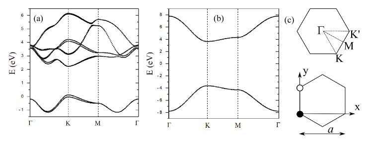
Figure 1: (a) TB-derived band structure (including SO coupling) of the MoS₂ monolayer according to the Slater-Koster scheme discussed in the text and reported earlier in Ref. Ridolfi et al., 2015. (The Fermi energy is set to 0.) (b) TB-derived band structure of hBN (spin-degenerate) according to the parameterization discussed in the text and reported in Ref. Galvani et al., 2016. (The Fermi energy is set to 0.) (c) Top: Illustration of the Brillouin zone for both MoS₂ and hBN. Bottom: Representation of our orientation of the honeycomb lattice in real space with the positions of the $A$ and $B$ sites highlighted by the filled and empty circles. While $A$ and $B$ represent the positions of N and B atoms in hBN, in the case of MoS₂, we can associate them with a top view of the Mo and S atoms, respectively.

II Methodology

The central goal is to compute the time-dependent polarization induced in a non-polar crystal, $\bm{P}(t)$ (dipole moment per unit area of the crystal), in response to a time-dependent electromagnetic field, $\bm{E}(t)$. The field may have generic magnitude and time dependence (i.e., neither small nor sinusoidal), and we wish the computed $\bm{P}(t)$ to include the major effects of electron-electron interactions — fundamental for an adequate description of the optical properties of 2D semiconductors, where excitonic renormalization effects are very pronounced and dominate the optical spectra Thygesen (2017); Wang et al. (2018). In the most general terms, the response to a field of arbitrary strength is determined by the $n$-th order susceptibilities according to

$$\epsilon_{0}^{-1}P^{\lambda}(t) =\int^{t}\!\!dt_{1}\,\chi^{(1)}_{\lambda\alpha}(t,t_{1})E^{\alpha}(t_{1})$$

$$+\int^{t}\!\!dt_{1}\!\int^{t_{1}}\!\!\!dt_{2}\,\chi^{(2)}_{\lambda\alpha\beta}(t,t_{1},t_{2})E^{\alpha}(t_{1})E^{\beta}(t_{2})$$

$$+...,$$ (1)

where $\epsilon_{0}$ is the vacuum dielectric permittivity and $\lambda$, $\alpha$, $\beta$ are Cartesian components. Being non-perturbative, the calculated $\bm{P}(t)$ will contain the information of all nonlinear susceptibilities $\chi^{(n)}$ (which can be extracted by appropriate post-processing) with excitonic effects included from the outset. To capture microscopic coherence in $\bm{P}(t)$ to all orders in the external field requires a nonequilibrium framework Schmitt-Rink et al. (1988).

Our approach is strongly inspired by the technique and approximations proposed by Attaccalite et al. for a fully ab initio strategy to obtain the optical response in the time domain based on nonequilibrium GFs Attaccalite et al. (2011a). However, we depart from their original formulation by (i) considering a TB parameterization of the quasi-particle-renormalized Hamiltonian, as well as by (ii) describing the Coulomb interactions by a parameterized screened potential. This expedites the numerical time-integration and makes calculations at each time step less memory-demanding, especially if the desired energy range comprises many bands and/or a large number of $\bm{k}$ points in the sampling of the Brillouin zone (BZ). Our objective in the present paper is to explicitly show this approach to be both reliable and efficient.

Throughout this article we consider that the target system remains spatially homogeneous under the influence of the external radiation field. This is appropriate since the frequencies of interest are of the order of the optical bandgap (typically in the infrared-to-visible range), with associated wavelengths much larger than the atomic distances. As we concentrate on strictly 2D crystals, all our vector quantities are restricted to the $xy$ plane, which coincides with the crystalline sheet.

The polarization can be expressed in terms of the one-particle reduced density matrix as Resta (1994)

$$\bm{P}(t)=e\int\!\text{$\bm{r}$}\hat{\rho}(\text{$\bm{r}$})d\text{$\bm{r}$}=\frac{e}{A}\sum_{mn\text{$\bm{k}$}}\text{$\bm{r}$}_{mn\text{$\bm{k}$}}\,\rho_{mn\text{$\bm{k}$}}(t),$$ (2)

where $e<0$ is the charge of the electron; $A$ is the area of the crystal ($A=A_{c}N_{k}^{2}$ for $N_{k}^{2}$ unit cells and area per cell $A_{c}\equiv\sqrt{3}a^{2}/2$); $\rho_{mn\text{$\bm{k}$}}(t)\equiv\langle a^{\dagger}_{m\text{$\bm{k}$}}(t)a_{n\text{$\bm{k}$}}(t)\rangle$ is the reduced density matrix; the Heisenberg operator $a^{\dagger}_{m\text{$\bm{k}$}}(t)$ creates an electron in the Bloch eigenstate $\psi_{m\text{$\bm{k}$}}(\text{$\bm{r}$})\equiv\braket{\text{$\bm{r}$}}{m\text{$\bm{k}$}}$ at time $t$; $\text{$\bm{r}$}_{mn\text{$\bm{k}$}}\equiv\bra{m\text{$\bm{k}$}}\hat{\bm{r}}\ket{n\text{$\bm{k}$}}$. As we are interested in a non-equilibrium description, we introduce the two-time lesser GF Kadanoff and Baym (1962); Kremp et al. (2005) in the Bloch representation:

$$G^{<}_{mn\text{$\bm{k}$}}(t,t^{\prime})\equiv i\langle a^{\dagger}_{n\text{$\bm{k}$}}(t^{\prime})a_{m\text{$\bm{k}$}}(t)\rangle\\ =i\int\!\!d\text{$\bm{r}$}d\text{$\bm{r}$}^{\prime}\,\psi^{*}_{m\text{$\bm{k}$}}(\text{$\bm{r}$})\psi_{n\text{$\bm{k}$}}(\text{$\bm{r}$}^{\prime})\,\langle\hat{\psi}^{\dagger}(\text{$\bm{r}$}^{\prime},t^{\prime})\hat{\psi}(\text{$\bm{r}$},t)\rangle.$$ (3)

Here, $\hat{\psi}(\text{$\bm{r}$},t)$ represents the electronic field operator and $i\,\langle\hat{\psi}^{\dagger}(\text{$\bm{r}$}^{\prime},t^{\prime})\hat{\psi}(\text{$\bm{r}$},t)\rangle{\,\equiv\,}G^{<}(\text{$\bm{r}$}t,\text{$\bm{r}$}^{\prime}t^{\prime})$, which is the real-space representation of the lesser GF. Note that the time-diagonal component of $G^{<}_{mn\text{$\bm{k}$}}(t,t^{\prime})$ coincides with the reduced density matrix, $\hat{\rho}(t)$:

$$G^{<}_{mn\text{$\bm{k}$}}(t)\equiv\lim_{t^{\prime}\to t^{+}}G^{<}_{mn\text{$\bm{k}$}}(t,t^{\prime})=i\rho_{nm\text{$\bm{k}$}}(t).$$ (4)

Hence, Eq. (2) can be recast as

$$\bm{P}(t)=-\frac{ie}{A}\sum_{mn\text{$\bm{k}$}}\text{$\bm{r}$}_{mn\text{$\bm{k}$}}\,G^{<}_{nm\text{$\bm{k}$}}(t).$$ (5)

The central problem is thus determining the time dependence of $G^{<}_{nm\text{$\bm{k}$}}(t)$ under the influence of an external field of arbitrary strength and arbitrary temporal profile.

II.1 Equation of motion for the distribution function

Many-body electronic excitations in response to a time-dependent external field are most systematically handled with GF techniques. To obtain $\bm{P}(t)$ in a non-perturbative way implies that our description must properly handle arbitrarily strong fields (and, of course, in experiments, probing the nonlinear susceptibilities does require intense laser fields Boyd (2008)). Strong fields are bound to drive the statistical system out of thermodynamic equilibrium. An accurate description of the coherent microscopic processes therefore requires a nonequilibrium GF formalism Schmitt-Rink et al. (1988), which has been pioneered by Kadanoff and Baym Kadanoff and Baym (1962), and by Keldysh Keldysh (1964).

Since details related to the derivation of the equation of motion for $G^{<}_{nm\text{$\bm{k}$}}(t)$ have been discussed, for example, in Refs. Attaccalite et al., 2011a or Schmitt-Rink et al., 1988, we provide only a qualitative overview of its key aspects and assumptions. In addition to establishing the context for our numerical calculations in a conceptually self-contained way, this allows us to highlight the necessary adaptations necessary for our approach, which is based on parameterized Hamiltonians and interactions.

Kadanoff and Baym provided a closed set of coupled equations for the time evolution of the different nonequilibrium GFs in terms of self-energies defined on distinct portions of the Keldysh contour; for practical calculations, the self-energies must be specified within an approximation scheme Kadanoff and Baym (1962); Kremp et al. (2005). A major simplifying step occurs by approximating $\Sigma^{<}=0$ and $\Sigma^{r}=\Sigma^{a}\equiv\Sigma$, similarly to what happens in a collisionless and instantaneous scenario like Hartree-Fock Schmitt-Rink et al. (1988). The equation for $G^{<}_{nm\text{$\bm{k}$}}(t)$ then decouples and reads Attaccalite et al. (2011a); Schmitt-Rink et al. (1988):

$$i\hbar\frac{\partial}{\partial t}\bm{G}_{\text{$\bm{k}$}}^{<}(t)=\Bigl{[}\bm{h}_{\text{$\bm{k}$}}+\bm{U}_{\text{$\bm{k}$}}(t)+\bm{\Sigma}_{\text{$\bm{k}$}}[\bm{G}_{\text{$\bm{k}$}}^{<}(t)],\bm{G}_{\text{$\bm{k}$}}^{<}(t)\Bigr{]},$$ (6)

where $[\bm{A},\bm{B}]\equiv\bm{A}\bm{B}-\bm{B}\bm{A}$. For notational simplicity, we employ bold symbols to denote matrices in the band indices: for example, $G_{mn\text{$\bm{k}$}}^{<}(t)=[\bm{G}_{\text{$\bm{k}$}}^{<}(t)]_{mn}$, and $h_{mn\text{$\bm{k}$}}=[\bm{h_{\text{$\bm{k}$}}}]_{mn}=\bra{m\text{$\bm{k}$}}\hat{h}\ket{n\text{$\bm{k}$}}=\delta_{mn}E_{m\text{$\bm{k}$}}$, where $E_{m\text{$\bm{k}$}}$ are the Bloch bands.

The electronic system is defined here by the non-interacting Bloch Hamiltonian $\hat{h}$, and $\hat{U}(t)$ is the explicitly time-dependent external field. The total non-interacting Hamiltonian is thus

$$\hat{H}(t)=\hat{h}+\hat{U}(t).$$ (7)

Eq. (6) extends the most commonly employed framework known as “semiconductor Bloch equations” (the dynamical equations for the reduced density matrix) Schäfer and Wegener (2002); Aversa and Sipe (1995) with the addition of a self-energy $\hat{\Sigma}$, which can be non-Hermitian to capture relaxation processes. While the semiconductor Bloch equations are an equation-of-motion approach to the time evolution of $\hat{\rho}$ Schäfer and Wegener (2002), our formulation in terms of GFs and self-energies is best suited (through the machinery or GFs and diagramatics) for systematic study of different interaction and relaxation mechanisms without additional formal effort. The self-energy encodes all the many-body correlation and decoherence (in the imaginary part) effects; as these depend on the electronic occupations, $\hat{\Sigma}$ is a functional of $G_{mn\text{$\bm{k}$}}^{<}(t)$ which is represented by the term $\bm{\Sigma}_{\text{$\bm{k}$}}[\bm{G}_{\text{$\bm{k}$}}^{<}(t)]$ in Eq. (6).

We note that the Hamiltonian $\hat{h}$ is meant to be described in terms of a TB parameterization; but having it reflect the strictly non-interacting Bloch Hamiltonian is not optimal, for two main reasons. On the one hand, irrespective of whether the TB Hamiltonian is obtained from a DFT calculation or constrained directly by experiments, it will already incorporate electron-electron interactions (in the DFT case, the TB parameterization reflects at least the Kohn-Sham Hamiltonian, which already incorporates interactions at a basic level). On the other hand, it is desirable that $\hat{h}$ provides an accurate description of the ground state; in the case of a semiconductor — and particularly so for 2D materials — that requires incorporating the interaction-driven corrections to the quasiparticle dispersion beyond DFT Hybertsen and Louie (1986). Therefore, we take $\hat{h}$ and its spectrum, $E_{m\text{$\bm{k}$}}$, to represent a TB parameterization of the ground state band structure which already takes into account such corrections — for example, at the level of the $GW$ approximation Hedin and Lundqvist (1970); Hybertsen and Louie (1986), or as provided by hybrid functional approaches to DFT Becke (1993).

These considerations require a corresponding and consistent reassessment of the self-energy term in Eq. (6) to avoid double-counting of interactions. We hence rewrite that equation as

$$i\hbar\frac{\partial}{\partial t}\bm{G}_{\text{$\bm{k}$}}^{<}(t)=\Bigl{[}\bm{H}_{\text{$\bm{k}$}}(t)+\bm{\Sigma}_{\text{$\bm{k}$}}[G^{<}(t)]-\bm{\Sigma}_{\text{$\bm{k}$}}[\tilde{G}^{<}],\,\bm{G}_{\text{$\bm{k}$}}^{<}(t)\Bigr{]},$$ (8)

where $\tilde{G}^{<}$ represents the GF of the unperturbed system at equilibrium,

$$\tilde{G}^{<}_{mn\text{$\bm{k}$}}\equiv G^{<}_{mn\text{$\bm{k}$}}(t=0)=i\delta_{mn}f_{m\text{$\bm{k}$}},$$ (9)

and $f_{m\text{$\bm{k}$}}$ is the Fermi-Dirac distribution at energy $E_{m\text{$\bm{k}$}}$. The effect of the term $-\bm{\Sigma}_{\text{$\bm{k}$}}[\tilde{G}^{<}]$ is to subtract from the self-energy the quasiparticle corrections of the unperturbed system at equilibrium (which, according to the above discussion, should be already included in the TB parameterization for $\hat{h}$). In this way, the self-energy terms describe only the correlation changes induced by the external field. Equation (8) is our counterpart of Eq. (11) proposed by Attaccalite et al. in Ref. Attaccalite et al., 2011a.

Note that the temperature only appears in the time evolution implicitly, via the Fermi-Dirac distribution that defines the initial condition (9). Zero and finite temperature calculations are thus on equal footing. Despite this, in the current work we set $T=0$ since we will benchmark our results against other zero-temperature calculations.

II.2 Tight-binding parameterizations

We rely on orthogonal TB Hamiltonians in the Slater-Koster formulation Slater and Koster (1954) to represent $\hat{h}$, where the Bloch eigenstates states, $\psi_{n\text{$\bm{k}$}}(\text{$\bm{r}$})$, are expanded in terms of effective local atomic orbitals, $\phi_{\alpha}(\text{$\bm{r}$})$, as follows:

$$\psi_{n\text{$\bm{k}$}}(\text{$\bm{r}$}) =\sum_{\alpha}C_{\alpha\text{$\bm{k}$}}^{n}\,\chi_{\alpha\text{$\bm{k}$}}(\text{$\bm{r}$}),$$

$$\chi_{\alpha\text{$\bm{k}$}}(\text{$\bm{r}$}) \equiv\frac{1}{\sqrt{N_{c}}}\sum_{\text{$\bm{R}$}}e^{i(\text{$\bm{k}$}\cdot\text{$\bm{R}$}+\theta_{\alpha\text{$\bm{k}$}})}\phi_{\alpha}(\text{$\bm{r}$}-\text{$\bm{R}$}-\text{$\bm{t}$}_{\alpha}).$$ (10)

The lattice vector $\bm{R}$ runs over all $N_{c}$ unit cells of the crystal, $n$ is the band index, $\alpha$ labels different orbitals within the unit cell which are centered at position $\text{$\bm{t}$}_{\alpha}$ relative to the cell’s origin. Both $n$ and $\alpha$ run over the interval $[1,N]$, where $N$ is the dimension of the orbital basis considered. Although the phase factor $\theta_{\alpha\text{$\bm{k}$}}$ can be fixed arbitrarily (for example $\theta_{\alpha\text{$\bm{k}$}}=0$), one has to consistently carry that choice to the matrix elements of the dipole operator and screened Coulomb interaction (to be discussed below). For convenience we set $\theta_{\alpha\text{$\bm{k}$}}=\text{$\bm{k}$}\cdot\text{$\bm{t}$}_{\alpha}$ everywhere in this work Ventura et al. (2019).

The specific TB parameterizations used in our calculations for MoS₂ and BN will be discussed further below. The underlying bandstructures are shown in Fig. 1.

II.3 External field

We express the perturbation due to the external radiation field, $\bm{E}(t)$, in the dipole approximation and length gauge Aversa and Sipe (1995):

$$\hat{U}(t)\equiv-e\,\hat{\text{$\bm{r}$}}\cdot\bm{E}(t).$$ (11)

Its matrix elements in the Bloch basis are $U_{mn\text{$\bm{k}$}}(t)=-e\,\text{$\bm{r}$}_{mn\text{$\bm{k}$}}\cdot\bm{E}(t)$ and thus require the computation of $\text{$\bm{r}$}_{mn\text{$\bm{k}$}}\equiv\bra{m\text{$\bm{k}$}}\hat{\text{$\bm{r}$}}\ket{n\text{$\bm{k}$}}$. We shall consider only inter-band transitions and neglect all intra-band matrix elements, $\text{$\bm{r}$}_{mm\text{$\bm{k}$}}$ (this point is revisited later). In that case, from the definition of the velocity operator $i\hbar\hat{\bm{v}}=[\hat{\text{$\bm{r}$}},\hat{h}]$, we have $\text{$\bm{r}$}_{mn\text{$\bm{k}$}}=i\hbar\bm{v}_{mn\text{$\bm{k}$}}/(E_{n\text{$\bm{k}$}}-E_{m\text{$\bm{k}$}})$. The matrix elements of the velocity can be approximated in the TB representation (10) as Pedersen et al. (2001)

$$\hbar\bm{v}_{mn\text{$\bm{k}$}}\simeq\sum_{\alpha\beta}C^{m*}_{\alpha\text{$\bm{k}$}}C^{n}_{\beta\text{$\bm{k}$}}\nabla_{\text{$\bm{k}$}}\bra{\chi_{\alpha\text{$\bm{k}$}}}\hat{h}\ket{\chi_{\beta\text{$\bm{k}$}}},$$ (12)

where $\bra{\chi_{\alpha\text{$\bm{k}$}}}\hat{h}\ket{\chi_{\beta\text{$\bm{k}$}}}$ are the matrix elements of the TB Hamiltonian in the reduced Bloch representation. In a Slater-Koster framework, their $\bm{k}$-dependence is explicitly known and, consequently, the $\bm{k}$-derivative appearing in Eq. (12) can be directly computed once the TB Hamiltonian is specified.

II.4 Self-energy approximation

The COHSEX (Coulomb hole and screened exchange) approximation of Hedin Hedin (1965) has been widely used to describe correlation effects in excited states Hybertsen and Louie (1986); Onida et al. (2002); Bruneval et al. (2006). It approximates the electronic self-energy as instantaneous in time and comprising two physical contributions: $\Sigma^{\text{cohsex}}=\Sigma^{\text{coh}}+\Sigma^{\text{sex}}$. The term

$$\Sigma^{\text{sex}}(\text{$\bm{r}$},\text{$\bm{r}$}^{\prime},t)\equiv iG(\text{$\bm{r}$}t;\text{$\bm{r}$}^{\prime}t^{+})\,W(\text{$\bm{r}$},\text{$\bm{r}$}^{\prime};\omega=0)$$ (13)

describes a statically screened exchange interaction, with $W(\text{$\bm{r}$},\text{$\bm{r}$}^{\prime};\omega)$ representing the dynamically screened Coulomb repulsion in the random-phase approximation, and

$$\Sigma^{\text{coh}}(\text{$\bm{r}$},\text{$\bm{r}$}^{\prime},t)\equiv\tfrac{1}{2}\delta(\text{$\bm{r}$}-\text{$\bm{r}$}^{\prime})\\ \times\Bigl{[}W(\text{$\bm{r}$},\text{$\bm{r}$}^{\prime};\omega=0)-w(\text{$\bm{r}$},\text{$\bm{r}$}^{\prime})\Bigr{]},$$ (14)

where $w(\text{$\bm{r}$},\text{$\bm{r}$}^{\prime})\equiv e^{2}/(4\pi\epsilon_{0}|\text{$\bm{r}$}-\text{$\bm{r}$}^{\prime}|)$ is the bare Coulomb repulsion. The instantaneous approximation to $\Sigma$ is justified in the present context because the self-energy in Eq. (8) is only operative in the presence of the external field. It therefore defines the strength of the electron-hole interaction but not the quasiparticle renormalization of the Kohn-Sham bandstructure. (While dynamical screening is crucial to obtain the correct quasiparticle renormalization Hybertsen and Louie (1986); Onida et al. (2002), in our formulation, that effect is already encoded in $\hat{h}$, by construction.) Furthermore, an instantaneous self-energy is in line with the current understanding, at the level of the BSE, that it correctly captures the excitonic spectrum of semiconductors — because of the excitons’ relatively long time-scales in comparison with the dynamical charge oscillations involved in screening Rohlfing and Louie (2000); Schöne and Ekardt (2002); Marini and Del Sole (2003).

Recalling the reasoning above for the subtraction in Eq. (10) of the self-energy calculated at equilibrium, we see that the contribution $\Sigma^{\text{coh}}$, being time-independent in this approximation, does not contribute to the time evolution of the distribution function defined by Eq. (10). We therefore need only to consider the screened exchange contribution (13). In this regard, note that the approximation in Eq. (13) for $\Sigma^{\text{sex}}$ consists in a static $GW$ approximation Onida et al. (2002); hence, if the term $-\Sigma[\tilde{G}^{<}]$ were not included in Eq. (8), one would be doubly correcting the quasiparticle bandstructure renormalization.

Our approximation to the self-energy therefore reads

$$\Sigma_{mn\text{$\bm{k}$}}\bigl{[}G^{<}(t)\bigr{]}=i\sum_{jl\text{$\bm{k}$}^{\prime}}W_{mn\text{$\bm{k}$},\,jl\text{$\bm{k}$}^{\prime}}\,G_{jl\text{$\bm{k}$}^{\prime}}^{<}(t)$$ (15)

in an explicit Bloch representation. The matrix elements of the screened exchange interaction are defined as

$$W_{mn\text{$\bm{k}$},jl\text{$\bm{k}$}^{\prime}}\equiv\int\!\!d\text{$\bm{r}$}d\text{$\bm{r}$}^{\prime}\,\psi_{m\text{$\bm{k}$}}^{*}(\text{$\bm{r}$})\psi_{l\text{$\bm{k}$}^{\prime}}^{*}(\text{$\bm{r}$}^{\prime})\\ \times W(\text{$\bm{r}$}-\text{$\bm{r}$}^{\prime})\psi_{j\text{$\bm{k}$}^{\prime}}(\text{$\bm{r}$})\psi_{n\text{$\bm{k}$}}(\text{$\bm{r}$}^{\prime}).$$ (16)

In the TB basis introduced in (10), these matrix elements read explicitly Trolle et al. (2014); Ridolfi et al. (2018); Trevisanutto and Vignale (2016)^,

$$W_{mn\text{$\bm{k}$},jl\text{$\bm{k}$}^{\prime}}\equiv\sum_{\text{$\bm{G}$}}{[I^{\text{$\bm{G}$}}_{j\text{$\bm{k}$}^{\prime},m\text{$\bm{k}$}}]}^{*}\,I^{\text{$\bm{G}$}}_{l\text{$\bm{k}$}^{\prime},n\text{$\bm{k}$}}\;W(\text{$\bm{k}$}-\text{$\bm{k}$}^{\prime}+\text{$\bm{G}$}),$$ (17)

where $W(\text{$\bm{q}$})$ represents the zero-frequency limit of the screened Coulomb potential,

$$W(\text{$\bm{q}$})\equiv\biggl{(}\frac{e^{2}}{2\epsilon_{0}\epsilon_{d}A}\biggr{)}\frac{1}{|\text{$\bm{q}$}|\,(1+\lambda_{0}|\text{$\bm{q}$}|)}.$$ (18)

This expression corresponds to the regime of small $\bm{q}$ calculated for a strictly 2D electron gas embedded in three dimensions Keldysh (1979); Cudazzo et al. (2011); Trolle et al. (2017). $A$ is the area of the crystal, $\lambda_{0}$ its 2D polarizability Cudazzo et al. (2011); Chernikov et al. (2014); Rodin et al. (2014), and $\epsilon_{d}$ captures the average dielectric constant of the environment. For us, in practice, $\epsilon_{d}=(\epsilon_{1}+\epsilon_{2})/2$ to capture the effect of static, uniform screening due to the top ($\epsilon_{1}$) and bottom ($\epsilon_{2}$) media surrounding the target 2D crystal. The parameters $\epsilon_{d}$ and $\lambda_{0}$ must be given to completely specify the screened interaction (18).

The Bloch coherence factors appearing in Eq. (17) are defined as

$$I^{\text{$\bm{G}$}}_{m\text{$\bm{k}$},m^{\prime}\text{$\bm{k}$}^{\prime}} \equiv\bra{m\text{$\bm{k}$}}e^{i(\text{$\bm{k}$}-\text{$\bm{k}$}^{\prime}-\text{$\bm{G}$})\cdot\hat{\text{$\bm{r}$}}}\ket{m^{\prime}\text{$\bm{k}$}^{\prime}}$$ (19)

$$=\int d\text{$\bm{r}$}\,\psi^{*}_{m\text{$\bm{k}$}}(\text{$\bm{r}$})e^{i(\text{$\bm{k}$}-\text{$\bm{k}$}^{\prime}-\text{$\bm{G}$})\cdot\hat{\text{$\bm{r}$}}}\psi_{m^{\prime}\text{$\bm{k}$}^{\prime}}(\text{$\bm{r}$})$$

Expanding for the Bloch functions introduced in Eq. (10) yields

$$I^{\text{$\bm{G}$}}_{m\text{$\bm{k}$},m^{\prime}\text{$\bm{k}$}^{\prime}}\simeq\sum_{\alpha}[\,C_{\alpha\text{$\bm{k}$}}^{m}e^{i\theta_{\alpha\text{$\bm{k}$}}}\,]^{*}\,[\,C_{\alpha\text{$\bm{k}$}^{\prime}}^{m^{\prime}}e^{i\theta_{\alpha\text{$\bm{k}$}^{\prime}}}\,]\\ \times e^{i(\text{$\bm{k}$}-\text{$\bm{k}$}^{\prime}-\text{$\bm{G}$})\cdot\text{$\bm{t}$}_{\alpha}}.$$ (20)

The vectors $\bm{G}$ in the above expressions belong to the reciprocal lattice. However, we emphasize that they do not reflect any attempt to include local-field corrections, which would not be warranted in our Slater-Koster TB scheme. The sum over $\bm{G}$ is needed in Eq. (17) to restore the symmetry in the interaction between an electron with crystal momentum $\bm{k}$ and another with $\text{$\bm{k}$}^{\prime}$: Since $\text{$\bm{k}$},\text{$\bm{k}$}^{\prime}$ are restricted to the first BZ — but the Fourier components of the Coulomb interaction are not — the interaction should include not only $\bm{k}$ and $\text{$\bm{k}$}^{\prime}$ but all the equivalent pairs of crystal momenta. The decay of $W(\text{$\bm{q}$})$ justifies retaining only $\text{$\bm{G}$}=0$ in most cases. However, in 2D materials the exciton binding energies can be extremely large — this implies tightly bound excitons in real space and, consequently, slowly decaying wavefunctions in reciprocal space. Consequently, the wavefunctions of an exciton at the $K$ valley and another at $K^{\prime}$ can overlap, which might lead to a non-negligible Coulomb matrix element between those states. In such cases, the absence of the equivalent valleys beyond the first BZ amounts to an artificial symmetry breaking in the system — the summation over $\bm{G}$ ensures such symmetry is retained. In practice, we keep only the fewest $\bm{G}$ necessary to obtain converged results. (While in the calculations for MoS₂ we found that including only $\text{$\bm{G}$}=0$ is sufficient, additional vectors were found to be important in the case of hBN, and we will return to this point later.)

Finally, we point out that in the proposal to implement this scheme fully ab initio Attaccalite et al. (2011a) — where $\hat{h}$ represents the Kohn-Sham Hamiltonian obtained as a first step within DFT — the Hartree energy must be updated at every time step as well for consistency. In our formulation, the Hartree term does not play a role under the time evolution. This is motivated by the fact that, in a BSE approach to the two-particle problem at $T=0$, the Hartree term in the Hamiltonian (7) generates the so-called “exchange” interaction in the BSE Rohlfing and Louie (2000), whose matrix elements have the form

$$\int\!\!d\text{$\bm{r}$}\,\psi_{c\text{$\bm{k}$}}^{*}(\text{$\bm{r}$})\psi_{v\text{$\bm{k}$}}(\text{$\bm{r}$})w(\text{$\bm{r}$}-\text{$\bm{r}$}^{\prime})\psi_{v\text{$\bm{k}$}^{\prime}}^{*}(\text{$\bm{r}$}^{\prime})\psi_{c\text{$\bm{k}$}^{\prime}}(\text{$\bm{r}$}^{\prime}),$$ (21)

where the labels $c$/$v$ stand for indices that run over the conduction/valence bands only. When written in Fourier space, and neglecting local-field corrections, this expression reduces to $w(\text{$\bm{q}$}{\,=\,}0)\delta_{cv}\delta_{c^{\prime}v^{\prime}}$. But the Kronecker delta $\delta_{vc}=0$ because a conduction band can never coincide with a valence one. Hence, the Hartree contribution drops from the BSE, which means it is irrelevant for excitonic effects (this is also the reason why, even when one does take local-field effects into account, the Hartree contribution tends to be much smaller than that arising from the screened exchange interaction). By definition, an orthogonal TB expansion of the Bloch states such as Eq. (10) ignores local-field corrections. Therefore, in our formulation the Hartree contribution remains implicitly as part of $\hat{h}$ without dynamical updates.

We wish to emphasize two important aspects of this strategy to tackle the interaction effects. The first is that, by formulating the problem in the form of Eq. (8) where the self-energy dictates all interaction and/or relaxation effects, a multitude of extensions to the current approximations is straightforward — it requires only the specification of additional terms in the self-energy, but not an overhaul of the implementation. Hence, this formulation is intrinsically versatile and adaptable. (The most interesting extensions would arguably be to include the influence of coupling to other degrees of freedom, such as phonons, or specific models of disorder as physical sources of broadening.) The second aspect relates to the specific approximation for our self-energy in Eq. (15): Ref. Attaccalite et al., 2011a shows that, in linear order on the external field, this approximation is equivalent to a combined $G_{0}W_{0}$+BSE approach, which is the state-of-the-art combination to reliably describe excitonic effects in semiconductors Rohlfing and Louie (2000); Onida et al. (2002). It is therefore the most promising basis to describe interaction effects in optical response beyond linear order.

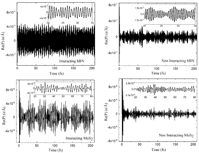
Figure 2: Time-dependent polarization calculated in response to a sub-fs optical pulse for a monolayer of hBN (top row) and MoS₂ (bottom). For comparison, we show results with (left) and without (right) the effect of Coulomb interactions. [For hBN: $t_{p}=0.15$ fs, $N_{c}=N_{v}=1$, $N_{k}^{2}=36^{2}$, $\tau=0.0125$ fs, $E_{0}=0.1$ mV/Å. For MoS₂: $t_{p}=0.3$ fs, $N_{c}=6$, $N_{v}=2$, $N_{k}^{2}=36^{2}$, $\tau=0.05$ fs, $E_{0}=0.1$ mV/Å.]

II.5 Fourier analysis of the optical response

To characterize the response in the frequency domain, we compute the discrete Fourier transform (FT) of the time-domain polarizability and electric fields. We define the discrete FT of a time-dependent signal $f(t)$ that is sampled at every constant interval $\tau$ as

$$F_{\omega_{k}}\equiv\frac{1}{L}\sum_{n=0}^{L-1}f(t_{n})e^{i\omega_{k}t_{n}},$$ (22)

where $t_{n}\equiv n\tau$, $L$ is the total number of time samples, $T\equiv L\tau$ is the total duration of the signal, and $\omega_{k}\equiv 2\pi k/T$ for $k\in\{0,1,...L-1\}$. It is obvious that the maximum frequency resolution of this procedure is $2\pi/T$ and, consequently, the total duration of the signal should in principle satisfy $T\gtrsim 2\pi/\gamma$ so that its Fourier spectrum has at least the resolution imposed by the characteristic broadening of the system, $\gamma$ [cf. Eq. (30) below] — this is one of the two compromises that ultimately determine the duration of the calculations in practice.

The other compromise is the time step, $\Delta t$, chosen to numerically integrate the equation of motion. Suppose, for example, that we wish to compute the response to a sinusoidal light field with a typical frequency of $\hbar\omega_{0}\sim 1$ eV (242 THz). It should be clear that, because of the oscillatory nature of the solution for $P(t)$, one must set $\Delta t$ to a fraction of the fundamental period of the driving field to avoid accumulating numerical errors. If, for definiteness, one assumes 10 integration steps per fundamental period, we have $\Delta t=2\pi/(10\omega_{0})\sim 0.4$ fs. If we now seek a frequency resolution of, say, $10$ meV, we must also have $2\pi\hbar/T\lesssim 10$ meV, or $T\gtrsim 1000\Delta t$. This means that the right-hand side of (8) must be evaluated at least 1000 times for such reasonable requirements. Of course, to ensure resolution of higher harmonics up to order $n$ of the fundamental frequency, one must replace $\omega_{0}\to n\omega_{0}$ in these estimates, whereby the numerical effort is seen to increase by a factor of $n$.

The choice of the time step has also the fundamental constraint imposed by the Nyquist-Shannon theorem: Since the $\Delta t$ used in the numerical integration defines the smallest possible sampling interval ($\min\tau=\Delta t$), the theorem imposes the maximum frequency captured in a discrete FT to be $\pi/\tau$ and, consequently, one must ensure $\Delta t\leq\tau<\pi/\omega_{\text{max}}$. As the energy scales of interest typically span several eV, $\Delta t$ must typically be well within the sub-fs range ($\hbar\pi/1\,\text{fs}\simeq 2.1$ eV) to allow a clean Fourier analysis (without aliasing, for example).

These compromises can make the numerical integration time-consuming (see also Section II.7 below). In contrast, the computation of the FTs appears “instantaneous” when compared with the total time spent integrating the polarization up to $t=T$. For this reason, our discrete FTs have been computed by sampling with $\tau=\Delta t$ to maximize the amount of information, and do not require any optimization beyond the prescription in Eq. (22).

Another advantage of computing the discrete FT as prescribed above using all the natural time steps from the numerical integration of Eq. (8) is that we can avoid the phenomenon of frequency leaking and ensure we always obtain an exact representation of the continuous FT of the signal $f(t)$ whenever it consists of a series of discrete frequencies (like in a monochromatic wave). In order to see this, we recall a simple result from Fourier analysis and signal processing. Let the continuous FT of a signal $f(t)$ be defined by

$$F(\omega)\equiv\frac{1}{2\pi}\int_{-\infty}^{+\infty}\!\!f(t)\,e^{i\omega t}dt.$$ (23)

$F(\omega)$ is related to $F_{\omega_{k}}$ defined in Eq. (22) through

$$F_{\omega_{k}}=\frac{2\pi}{T}\sum_{n=-\infty}^{+\infty}\Bigl{[}F(\omega-n\omega_{s})*\tilde{\delta}_{T/2}(\omega)\Bigr{]}_{\omega=\omega_{k}},$$ (24)

where $*$ represents the convolution operation, $\omega_{s}\equiv 2\pi/\tau$ is the angular sampling rate, and

$$\tilde{\delta}_{T/2}(\omega)\equiv\frac{Te^{i\omega T/2}}{2\pi}\text{sinc}\Bigl{(}\frac{\omega T}{2}\Bigr{)}$$ (25)

is the FT of the rectangle function defined as unity for $0\leq t\leq T$ and zero otherwise. Now, if the signal is monochromatic with a frequency $\omega_{0}<\omega_{s}$, we have $F(\omega)=F_{0}\,\delta(\omega-\omega_{0})$ and, from Eq. (24), follows that

$$F_{\omega_{k}}=\frac{2\pi}{T}F_{0}\,\tilde{\delta}_{T/2}(\omega_{k}-\omega_{0}).$$ (26)

Noting that $\tilde{\delta}_{T/2}(0)=T/(2\pi)$, the result (26) means that, by adapting the sampling rate $\omega_{s}$ (i.e., by chosing $\tau$) to $\omega_{0}$ (or vice-versa) such that $\omega_{0}$ is one of the frequencies $\{\omega_{k}\}$, we ensure that $F_{\omega_{k}=\omega_{0}}=F_{0}$ exactly and $F_{\omega_{k}}=0$ for all other discrete frequencies (i.e., the discrete FT recovers the exact Fourier spectrum of the signal without any frequency leaking). This can be an important when extracting high-harmonic Fourier components from $P(t)$, which can be orders of magnitude smaller than the fundamental harmonic — we thus need to exclude or minimize all spurious effects, such as the inevitable frequency leaking that appears whenever $\omega_{s}$ is not matched to the relevant frequencies in the system’s response signal.

Fourier analysis of $P(t)$ will be used to obtain the nonlinear susceptibilities $\chi^{(n)}$ defined in Eq. (1). In the frequency domain, that relation reads

$$\epsilon_{0}^{-1}P(\omega)=\sum_{n=1}^{\infty}\int\!\!d\omega_{1}\cdots\!\int\!\!d\omega_{n}\,\chi^{(n)}(\omega_{1},\dots,\omega_{n})\\ E(\omega_{1})\cdots E(\omega_{n})\,\delta(\omega-\textstyle\sum_{n}\omega_{n}).$$ (27)

By integrating Eq. (8) in the presence of an external monochromatic field of frequency $\omega_{0}$, followed by the above-described approach to the discrete Fourier analysis, we extract all the $n$-th harmonic susceptibilities at once by computing

$$\chi^{(n)}(\omega_{0})=\frac{P_{\omega_{k}=n\omega_{0}}}{(E_{\omega_{k}=\omega_{0}})^{n}\epsilon_{0}},$$ (28)

or the the associated optical conductivities: $\sigma^{(n)}(\omega_{0})=-i\omega_{0}\epsilon_{0}\chi^{(n)}(\omega_{0})$.

II.6 Relaxation and broadening

The electronic system described by the equation of motion (8) accumulates all the energy transferred by the external radiation field (the self-energy is Hermitian). The corresponding runaway growth of the system’s polarization can cause numerical problems if Eq. (8) needs to be integrated over a very large number of time steps.

A short-duration laser pulse is not numerically problematic in these conditions, as we shall see below. For the purposes of comparison with experiments using short-pulse excitation, one can incorporate a phenomenological energy broadening into the Fourier spectrum by a simple modification of Eq. (22):

$$P_{\omega_{k}}=\frac{1}{L}\sum_{n=0}^{L-1}P(t_{n})e^{i(\omega_{k}+i\gamma)t_{n}}.$$ (29)

In this way, broadening is introduced at the post-processing stage, where $\hbar\gamma$ defines the desired energy resolution (in our calculations we explicitly set it to the half-width at half-maximum of the lowest exciton peak that appears in the spectra used as reference to benchmark our results).

A scenario of continuous excitation without damping causes the amplitude of $\bm{P}(t)$ in the system to grow in time with a linear envelope, which introduces artifacts as $\omega\to 0$ in the numerical FT. In these cases, we found it desirable to introduce a phenomenological relaxation mechanism directly into the equation of motion (8), which is then modified to

$$i\hbar\frac{\partial}{\partial t}\bm{G}_{\text{$\bm{k}$}}^{<}(t)= \Bigl{[}\bm{H}_{\text{$\bm{k}$}}(t)+\bm{\Sigma}_{\text{$\bm{k}$}}[G^{<}(t)]-\bm{\Sigma}_{\text{$\bm{k}$}}[\tilde{G}^{<}],\,\bm{G}_{\text{$\bm{k}$}}^{<}(t)\Bigr{]}$$

$$-i\hbar\gamma\bigl{(}\bm{G}_{\text{$\bm{k}$}}^{<}(t)-\tilde{\bm{G}}_{\text{$\bm{k}$}}^{<}\bigr{)}.$$ (30)

The new term on the right-hand side promotes the return of the distribution function to equilibrium; the broadening parameter $\gamma$ is set to the target energy resolution as described above.

Of course, both approaches are employed here as a phenomenological strategy to control the energy broadening of the final results, which is sufficient for the current purposes of this paper. But, as pointed out earlier, more sophisticated and microscopically motivated relaxation processes may be incorporated directly into the equation of motion as extensions of Eq. (30) Wismer and Yakovlev (2018).

II.7 Implementation Notes

Numerical integration — After specifying the time dependence of the external field, we compute the time-dependent polarization according to (5). The set of coupled equations of motion represented by Eq. (8) is integrated numerically using the second-order Runge-Kutta algorithm provided within the GSL library M. Galassi et al. (2009). The choice of second-order is here a compromise between accuracy and expediency, since we wish to maintain the number of intermediate evaluations of the right-hand side of (8) as small as possible per time-step.

Problem dimension — It is instructive to recall that the linear dimension, $N_{\text{tot}}$ of the matrices in Eq. (8) is defined by the total number of bands ($N_{v}$ valence and $N_{c}$ conduction) plus the total number of $\bm{k}$ points that need to be sampled in the BZ. Therefore, $N_{\text{tot}}=N_{k}^{2}(N_{c}+N_{v})^{2}$, where $N_{k}^{2}$ represents the total number of $\bm{k}$ points ($N_{k}$ along each reciprocal direction). Since the Coulomb matrix elements (17) are non-diagonal in $\bm{k}$, their storage is the most costly since it requires $\sim N_{\text{tot}}^{2}/2$ entries in memory. Combining this with the fact that these matrices are to be multiplied several times for each time step of the Runge-Kutta integration leads to a numerical problem that quickly becomes challenging memory- and time-wise, even when considering minimal requirements of, say, $N_{k}=32$ and $N_{c}+N_{v}=2$.

Symmetry — We will focus on 2D crystals with threefold symmetry, having point-symmetry group $D_{3h}$ or higher. This already covers the materials that are currently most actively studied, such as graphene and its derivatives, hBN, transition-metal dichalcogenides, silicene, stanene, germanene, and several others. This restriction is practical, not fundamental. It is adopted here because their linear and second-harmonic (SH) susceptibility tensors are completely specified by computing only the diagonal component along $y$Boyd (2008). For our choice of lattice orientation in Fig. 1(c), symmetry imposes $\chi_{xx}^{(1)}=\chi_{yy}^{(1)}$ and $-\chi_{yyy}^{(2)}=\chi_{xxy}^{(2)}=\chi_{xyx}^{(2)}=\chi_{yxx}^{(2)}$. From this point onwards we thus drop the Cartesian indices: $\bm{P}\to P(t)\equiv P_{y}(t)$, $\bm{E}\to E(t)\equiv E_{y}(t)$, and $\chi_{\lambda\alpha\cdots}^{(n)}\to\chi^{(n)}\equiv\chi^{(n)}_{yy\cdots}$.

Nonlinear processes — We will address only the $n$-th harmonic susceptibilities in this paper, which are a function of only one frequency. Hence, we will also adopt a simplified notation $\chi^{(n)}(\omega_{1},\dots,\omega_{n})\to\chi^{(n)}(\omega)$ throughout the remainder of this paper, where the single frequency $\omega$ is that of the driving field (i.e., the fundamental frequency when the field is monochromatic).

Windowing — We found that applying a window function to our numerical time series for $P(t)$ considerably reduces the effect of the transient background due to the field switch-on, which is an important consideration when resolving the nonlinear contributions (to be discussed below). Windowing consists in multiplying the original signal by a so-called window function, $\zeta(t)$, which is chosen to provide a desired redistribution of its Fourier spectrum. (This technique is frequently used to minimize frequency leaking in discrete Fourier analysis Orfanidis (1996).) The Fourier analysis described in Section III.4 has been performed after applying a Hann window to the time-dependent polarization. In the notation of the previous section, this means replacing the time-dependent signal $f(t_{n})\longrightarrow f(t_{n})\,\zeta(t_{n})$, where the Hann window function is defined as

$$\zeta(t_{n})\equiv 2\,\sin^{2}\left(\frac{n\pi}{L-1}\right),\quad 0\leq n\leq L-1.$$ (31)

In this formulation, the window function defines the envelope of the total time series $f(t_{n})$. The Hann window does not introduce any additional parameter.

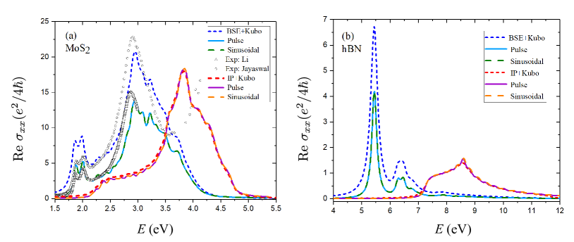
Figure 3: (a) Linear optical conductivity of MoS₂. The two curves represented by circles and triangles are experimental at room temperature Li et al. (2014); Jayaswal et al. (2018). The lines labeled “Pulse” refer to the optical conductivity obtained from Fourier analysis of the time-domain polarizations shown in Figs. 2(c) and 2(d). The “BSE+Kubo” (“IP+Kubo”) traces were obtained from the linear Kubo formula following the diagonalization of the Bethe-Salpeter (independent-particle Schrödinger, IP) equation for the same Hamiltonian. The “Sinusoidal” curves were calculated from the time-domain response to continuous monochromatic fields as described in the text. The broadening in our calculations was set to match that of the first exciton peak in the experimental traces shown in the figure. (b) Linear optical conductivity of hBN with the same labeling convention as in (a). [For MoS₂: $t_{p}=0.3$ fs, $N_{c}=6$, $N_{v}=2$, $N_{k}^{2}=36^{2}$, $\tau=0.05$ fs, $E_{0}=0.1$ mV/Å, $\hbar\gamma=0.05$ eV. For hBN: $t_{p}=0.15$ fs, $N_{c}=N_{v}=1$, $N_{k}^{2}=60^{2}$, $\tau=0.0125$ fs, $E_{0}=0.1$ mV/Å, $\hbar\gamma=0.1$ eV.]

III Illustration for MoS₂ and hBN

We illustrate the potential of this approach with the cases of MoS₂ and hBN, which have been chosen for different specific reasons. MoS₂ is the most widely studied representative of the family of 2D TMD semiconductors. It is now known that, except in the energy region of the bound A/B exciton series, the accurate description of the optical excitations across this family of compounds requires consideration of at least 6 conduction bands ($3\times 2$ for spin); this is due to the fact that the so-called C excitons involve contributions from the bands dispersing along $\Gamma$-K and $\Gamma$-M Qiu et al. (2013); Klots et al. (2014); Molina-Sánchez et al. (2015); Ridolfi et al. (2018) [cf. Fig. 1(a)]. Since the spin-orbit-induced splitting of these bands is crucial for many of the unusual features in these materials, such as spin-valley locking Xiao et al. (2012); Mak et al. (2012); Zeng et al. (2012); Wang et al. (2018), a minimal model to describe the optical properties up to the energies of the C excitons requires in principle $2\times(3+1)=8$ bands to cover an energy span of $\sim 3$ eV Trolle et al. (2014); Ridolfi et al. (2018). MoS₂ is then chosen as a representative of a system with a relatively demanding TB parameterization, and an example of how this approach can yield extremely good quantitative agreement with experiments and ab initio calculations. Our model for BN was deliberately selected to specifically analyze the opposite extreme of having only 2 bands in the problem; it will provide further insight into the role of the inter- and intra-band matrix elements of the dipole operator [cf. Section II.3].

III.1 Parameterization of Hamiltonians and interactions

To describe the quasi-particle-corrected electronic structure of MoS₂ [i.e., the Hamiltonian $\hat{h}$ in Eq. (8)] we consider the orthogonal Slater-Koster Hamiltonian proposed in Ref. Ridolfi et al., 2015, which has been already demonstrated to capture extremely well the experimental optical absorption spectrum in a direct solution of the BSE Ridolfi et al. (2018). It is built from an atomic basis comprising the three $p$ valence orbitals in each S and the five $d$ orbitals of Mo; since the spin-orbit coupling must necessarily be included to properly describe the splitting of the bands near the optical gap, the total dimension of the basis is then $N=22$. Additional details of this TB model are described elsewhere Ridolfi et al. (2015). The associated band structure is reproduced in Fig. 1(a), reflecting the insulating ground state of a pristine monolayer with a direct gap at the $K/K^{\prime}$ points. In order to directly compare our susceptibilities with experiments, a rigid blue-shift in the energies by $+0.07$ eV has been incorporated in all the results shown below, in line with the procedure originally discussed in Ref. Ridolfi et al., 2018.

For hBN, we resort to the orthogonal TB Hamiltonian parameterization proposed by Galvani et al.Galvani et al. (2016) as it provides a good description of the $GW$-corrected ab initio band structure around the fundamental gap. It is a simple two-band (spin-degenerate) Hamiltonian which, in the notation introduced in Eq. (12), reads

$$\bra{\chi_{\alpha\text{$\bm{k}$}}}\hat{h}\ket{\chi_{\beta\text{$\bm{k}$}}}\mapsto\begin{bmatrix}E_{b}&-t\,\varphi(\text{$\bm{k}$})^{*}\\ -t\,\varphi(\text{$\bm{k}$})&E_{n}\end{bmatrix}\!\!.$$ (32)

where $E_{b}=3.625$ eV represents the on-site energy at the boron atom, $E_{n}=-3.625$ eV that at the nitrogen, $t=2.30$ eV is the hopping integral, $\varphi(\text{$\bm{k}$})\equiv e^{i\text{$\bm{k}$}\cdot\bm{\delta}_{1}}+e^{i\text{$\bm{k}$}\cdot\bm{\delta}_{2}}+e^{i\text{$\bm{k}$}\cdot\bm{\delta}_{3}}$ with vectors $\bm{\delta}_{1}=\tfrac{a}{\sqrt{3}}(\tfrac{\sqrt{3}}{2},-\tfrac{1}{2})$, $\bm{\delta}_{2}=\tfrac{a}{\sqrt{3}}(0,1)$, $\bm{\delta}_{3}=\tfrac{a}{\sqrt{3}}(-\tfrac{\sqrt{3}}{2},-\tfrac{1}{2})$, and $a\simeq 2.5$ Å is the hBN lattice constant. The associated band structure is reproduced in Fig. 1(b). We note that this parameterization is accurate in the vicinity of the fundamental gap but does not faithfully reflect the actual dispersion over the entire BZ, especially near the $\Gamma$ point Arnaud et al. (2006); Galvani et al. (2016). This limits the range of validity of our TB parameterization to particle-hole excitations with less than $\sim 8\text{--}9$ eV. In both materials, $\hat{h}$ is diagonalized in a uniform grid with ${N_{k}}^{2}$ points on the first BZ depicted in Fig. 1(c).

For the purposes of benchmarking our calculations, the screened Coulomb interaction (18) is parameterized in different scenarios for each material: For MoS₂ we chose the environment’s dielectric constant as $\epsilon_{d}=2.5$, which is appropriate for the air/silica interface ($\epsilon_{1}=1$, $\epsilon_{2}=4$), and set the polarizability parameter $r_{0}=13.55$ Å, which is know to produce good agreement with the measured exciton binding energies Zhang et al. (2014); Ridolfi et al. (2018). In the case of hBN, we used $r_{0}=10$ Å as suggested from DFT results Galvani et al. (2016), while $\epsilon_{d}=1$ so that we can directly compare our results with existing calculations for a free-standing hBN monolayer in vacuum. Finally, while for MoS₂ we found that considering only $\text{$\bm{G}$}=0$ in the expressions for the Coulomb matrix element (17) is sufficient, the case of hBN required the inclusion of at least 16 reciprocal vectors to recover the correct symmetry and degeneracy of the lowest excitonic states at the $K$ and $K^{\prime}$ points.

III.2 Excitons in the linear and nonlinear optical response of MoS₂ and hBN

Prior to discussing our results, we briefly overview the general features and calculations of the impact of electronic interactions (excitons) in the optical response of our two target materials, focusing especially on the nonlinear response. MoS₂ has conduction and valence band extrema located at the two nonequivalent $K$ points of the hexagonal BZ. While the gap is indirect in multilayers, it is direct at those $K$ points for the monolayer Mak et al. (2010); Zhang et al. (2013). A strong spin-orbit coupling splits the valence bands near $K$, generating two families of bound excitonic states traditionally labeled A and B Li et al. (2014); Zhu et al. (2015); Qiu et al. (2013); Wang et al. (2018), and contributed primarily by the metal $d$ orbitals. The two A and B excitons ($E_{A}<E_{B}$) generate strong absorption peaks that define the optical absorption threshold at $E_{A}=1.8\pm 0.1$ eV for a monolayer on silica, as can be seen in Fig. 3(a) below. At higher energies, the absorption spectrum is dominated by the so-called C and D broad resonances that involve significant contributions from the chalcogen orbitals Qiu et al. (2013); Klots et al. (2014); Molina-Sánchez et al. (2015); Ridolfi et al. (2018).

Despite numerous studies of its linear optical response, there have been few experimental reports of the second and higher harmonic susceptibilities of MoS₂ over extended energy ranges. Examples are Refs. Malard et al., 2013 and Kumar et al., 2013 that report the SH emission of both monolayer and trilayer in the region of the C resonance, and Ref. Trolle et al., 2015 which reports similar measurements over the range $0.9\text{--}1.6$ eV, but in multilayers. SH calculations that include excitonic effects have been performed ab initio in Ref. Grüning and Attaccalite, 2014a and by Pedersen et al.Trolle et al. (2014), who used a perturbative formulation based on the solution of the BSE with a parameterized model analogous to ours. SH susceptibilities calculated with further simplified effective band models, applicable only to the region of the A and B peaks, have also been recently reported Glazov et al. (2017); Soh et al. (2018).

In relation to hBN, the $p_{z}$ orbitals on B and N define the highest valence and lowest conduction bands which are separated by a large direct gap at the $K/K^{\prime}$ points [see Fig. 1(b)]. Experimentally, the optical gap is seen at $5.8$ eV in bulk hBN Mamy et al. (1981); Watanabe et al. (2004) while values spanning $5.6\text{--}6.0$ eV have been reported in optical absorption measurements for monolayers on quartz Song et al. (2010); Kim et al. (2012); Wu et al. (2015b). Various excitonic characteristics and their impact in the optical response have been studied by DFT+$GW$+BSE ab initio methods Wirtz et al. (2006); Arnaud et al. (2006); Wirtz et al. (2008); Marini (2008); Attaccalite et al. (2011a, b); Yan et al. (2012); Grüning and Attaccalite (2014a); Cudazzo et al. (2016); Galvani et al. (2016); Koskelo et al. (2017); Ferreira et al. (2019); Attaccalite et al. (2018); Ref. Galvani et al., 2016 has provided, in addition, a real-space Wannier approximation to reduce the BSE to an effective exciton TB model. Pursuing a two-band model similar to that in Eq. (32) and a screened interaction, Pedersen has solved the BSE equation and computed the SH susceptibility using an equilibrium second-order perturbative framework, and emphasized the importance of intra-band matrix elements of the dipole operator Aversa and Sipe (1995) in a length-gauge formulation of the coupling to the light field.

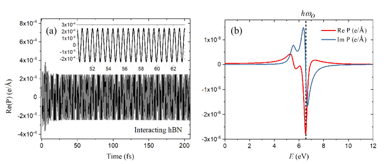
Figure 4: (a) Typical time-dependent polarization, $P(t)$, of a hBN monolayer in response to a continuous, monochromatic field with $\hbar\omega_{0}=6.65$ eV. (b) The corresponding Fourier spectrum, $P(\omega)$. The dashed line marks the frequency of the external field. [$N^{2}_{k}=36^{2}$, $N_{c}=N_{v}=1$, $E_{0}=10^{-2}$ V/Å, $\tau=0.0125$ fs, $\hbar\gamma=0.1$ eV]

III.3 Linear response to an optical pulse

The simplest perturbing field is that of a quasi-instantaneous pulse, which is particularly suitable to extract the linear response in a one-shot integration of Eq. (8). This is easily seen if one strictly sets $E(t)=E_{0}\delta(t)$ in Eq. (27) and ensures that $E_{0}$ is small; in lowest order

$$P(\omega)\simeq\frac{E_{0}}{2\pi\epsilon_{0}}\chi^{(1)}(\omega).$$ (33)

Therefore, since an instantaneous pulse excites the system equally at all frequencies, the Fourier transform of $P(t)$ computed as the response to a single instantaneous pulse directly yields the linear susceptibility at all frequencies. We followed this approach to demonstrate that the results obtained by integrating the equation of motion (8) reproduce the linear susceptibility computed from direct diagonalization of the BSE combined with the Kubo formula. Note that, in general, once the linear response is established, the nonlinear susceptibilities are immediately defined as well since they are obtained from the same time-dependent polarizability of the system, as indicated in Eq. (28). This is particularly true with regards to the absolute magnitudes of the high-order susceptibilities because, by ensuring that the linear susceptibility is quantitatively accurate, we can subsequently rely on the predicted magnitude of the higher-order components.

To appreciate the details of the implementation, it is instructive to walk through some of its key aspects and intermediate results, which we will now do in relation to the response of a short-duration pulse. For the numerical implementation, we shaped the pulse as an inverted parabola,

$$E(t)=E_{0}(t_{p}-t)t/t_{p}^{2},\quad 0\leq t\leq t_{p},$$ (34)

and $E(t)=0$ beyond $t_{p}$. The amplitude was kept at $E_{0}=10^{-4}$ V/Å and we verified that nonlinear effects are absent in the range $E_{0}\sim 1\text{--}10$ V/Å, which is consistent with the expectation that, in general, nonlinear effects emerge when the field strength approaches the magnitude characteristic of atomic electric fieldsBoyd (2008): $E_{\text{at}}=e/(4\pi\epsilon_{0}a_{0}^{2})\simeq 51$ V/Å.

Figure 2 shows the temporal profile of the induced polarization which has been integrated up to times in excess of 200 fs after the initial excitation with the pulse (34) ($t_{p}=0.15$ fs for hBN; $t_{p}=0.3$ fs for MoS₂). The main panels show the total time series for $P(t)$ in both systems with and without the effect of the screened Coulomb self energy in the calculation. It is visible that $P(t)$ remains finite and undamped, reflecting the fact that this calculation did not include relaxation terms [i.e., $\gamma=0$ in Eq. (30)]. Even without a detailed Fourier analysis, the time-domain picture reveals physically consistent signatures of the system’s expected behavior: For example, we can identify by direct inspection an average period of $\sim 0.48$ fs for hBN and $\sim 1.0\text{--}1.4$ fs for MoS₂ in the non-interacting polarizations [see insets of Figs. 2(b) and (d)]. These translate into characteristic energies of $\sim 8.6$ eV and $\sim 3\text{--}4$ eV, respectively, which coincide with the energies at which the non-interacting absorption spectrum is maximal in each case (cf. Fig. 3 below).

From a Fourier analysis of the $P(t)$ traces, we obtained the optical conductivities labeled “pulse” in Fig. 3. The broadening was introduced as per Eq. (29) where we used the experimental width $\hbar\gamma\simeq 0.07$ eV for MoS₂ and $\hbar\gamma=0.1$ eV for BN. The plot in Fig. 3(a) pertains to MoS₂ and exhibits two types of comparison. The two traces represented by points were extracted from the experimental reports in Refs. Li et al., 2014 and Jayaswal et al., 2018 for monolayers on SiO₂ substrates — one sees that our result reflected in the line labeled “pulse” describes all the experimental features very well, in particular the energies and spectral weight in the entire range of energies captured by our TB Hamiltonian ($\hbar\omega\lesssim 3.5$ eV). The trace labeled “perturbative” has been computed by a direct application of the linear Kubo formula to the spectrum of the BSE (for exactly the same TB Hamiltonian and parameterized interaction used here) as described earlier in Ref. Ridolfi et al., 2018. Finally, for reference and to further reinforce the substantial restructuring of the absorption spectrum brought about by the Coulomb interaction, the plot includes the conductivities obtained at the independent particle (IP) level (i.e., without the Coulomb self-energy). In quantitative terms, from the “impulse” curves we extract a quasiparticle band gap of $2.18$ eV and the lowest A/B excitons at $E_{A}=1.87$ eV and $E_{B}=2.00$ eV (binding energies $E^{b}_{A}=0.32$ eV and $E^{b}_{B}=0.34$ eV, respectively). This tallies well with results from angle-resolved photoemission spectroscopy Zhang et al. (2014), as well as X-ray photoemission and scanning tunneling spectroscopy Chiu et al. (2015), which place the band gap within $2.15\text{--}2.35$ eV; this yields binding energies in the range $0.22\text{--}0.42$ eV for the lowest A exciton.

The plots shown in Fig. 3(b) reflect the corresponding calculations applied to the case of hBN. For reference, our explicit diagonalization of the BSE yields the lowest excitonic levels with the following energies and degeneracies (in eV): {$5.44\,(\times 2)$, $5.96\,(\times 1)$, $6.27\,(\times 2)$, $6.28\,(\times 1)$, $2.45\,(\times 2)$}. As the quasiparticle band gap defined by our parameterization (32) is $7.25$ eV, the binding energies of these excitonic levels are, respectively, {$1.81$, $1.29$, $0.98$, $0.97$, $0.80$} eV. These figures compare reasonably well with those reported in Refs. Galvani et al., 2016 and Wirtz et al., 2008 using DFT+$GW$+BSE. Similarly to our result for MoS₂, the optical conductivity obtained for hBN with the time-domain framework reproduces the perturbative result, thereby validating our current implementation and the approximations involved. A characteristic of hBN is that the optical spectral weight is almost entirely concentrated at the exciton peaks, and is strongest at the lowest bright exciton. Indeed, the frequency dependence seen in Fig. 3(b) reproduces extremely well the quantitative and qualitative features of the absorption spectrum obtained by several other groups Arnaud et al. (2006); Wirtz et al. (2008, 2006); Marini (2008); Yan et al. (2012); Attaccalite et al. (2011a); Pedersen (2015); Galvani et al. (2016); Ferreira et al. (2019), and is compatible with the optical gaps of $5.6\text{--}6.0$ eV reported experimentally Song et al. (2010); Kim et al. (2012); Wu et al. (2015b). (Recall that we parameterized hBN in vacuum and, hence, both the $GW$ quasiparticle renormalization and the exciton binding would have to be adapted for a direct comparison with experiments.) Moreover, the absolute magnitude at the lowest exciton peak is here $\sigma^{(1)}(\omega=5.4)\simeq 4\,e^{2}/(4\hbar)$; this converts to an imaginary dielectric constant $\operatorname{Im}\varepsilon(\omega)=\operatorname{Re}\sigma^{(1)}(\omega)/(d\epsilon_{0}\omega)\simeq 10$ (using $d=3.3$ Å for effective thickness of a BN monolayer), which is entirely in line with the magnitude reported for this peak from first principles in Refs.Arnaud et al., 2006; Ferreira et al., 2019, as well as in optical absorption experiments with bulk BN Mamy et al. (1981).

Common to both materials (and, by extension, to all 2D semiconducting materials) is the fact that, if one were to ignore the Coulomb interaction effects, the predicted absorption spectrum would be patently inaccurate: (i) it would appear with a large overall blue-shift [cf. non-interacting curves]; (ii) it would entirely miss the excitonic spectral weight that dominates near the absorption threshold.

In the context of this paper, the most significant aspect of the results shown in Fig. 3 is that the time-domain calculation recovers the linear response function obtained perturbatively for the same microscopic parameterization of the system. We are thus in a position to explore the real power of the time-domain framework: its ability to naturally capture the response to arbitrary time-dependent fields, as well as to describe the nonlinear response in a rather expedite manner.

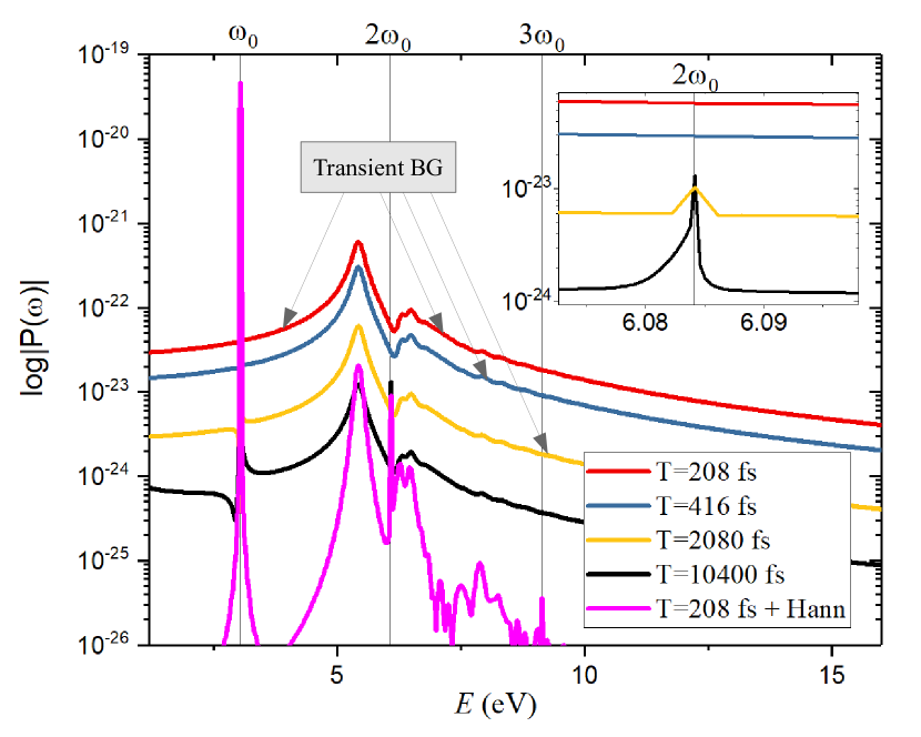
Figure 5: Frequency spectrum of $|P(\omega)|$ for hBN as a function of the duration of excitation (total integration time, $T$) by a continuous, monochromatic wave ($\hbar\omega_{0}=3.04$ eV). The spikes at $n\omega_{0}$ define the amplitude of the $n$-th harmonic charge oscillations. Note how the peak at $2\omega_{0}$ remains occluded by the transient tail (follow the arrows labeled “transient BG”) up to $T\sim 2080$ fs (inset), and how the transient background is suppressed $\propto 1/T$ with increasing $T$. The four topmost curves reflect the raw frequency spectrum (without windowing); the bottom-most (magenta) illustrates the advantage of using a Hann window, which allows resolving up to the third harmonic with only $T=208$ fs (without windowing, the trend from the other curves shows that $T$ would have to be ${\sim\,}10^{5}$ fs to resolve the third harmonic). Note that the vertical scale is logarithmic. [$N^{2}_{k}=36^{2}$, $N_{c}=N_{v}=1$, $E_{0}=0.01$ V/Å, $\tau=0.0125$ fs, $\hbar\gamma=0.1$ eV]

 

III.4 Nonlinear response to monochromatic fields

By definition, the high-harmonic susceptibilities $\chi^{(n)}(\omega_{0})$ in Eq. (28) represent the $n$-th order response of a system to a continuous, monochromatic wave at that frequency. More precisely, under a monochromatic perturbation of frequency $\omega_{0}$, the quantities $\chi^{(n)}(\omega_{0})$ evaluated at the single frequency $\omega_{0}$ are sufficient to entirely specify the time or frequency dependence of the polarization. This offers a direct way to compute the high-harmonic susceptibilities by sending a light field

$$E(t)=E_{0}\sin(\omega_{0}t),\qquad 0\leq t\leq T,$$ (35)

computing $P(\omega)$, and repeating for as many frequencies $\omega_{0}$ as desired Attaccalite and Grüning (2013). Of course, each calculation for a given frequency requires roughly the same duration as that for a quasi-instantaneous pulse which we described above. Therefore, the total time required to map $\chi^{(n)}(\omega)$ over a finite interval of frequencies will be comparatively much larger, in general, if a large number of frequencies is sought (by a factor that is roughly the number of such frequencies). Hence, despite the simplicity involved in extracting each $\chi^{(n)}(\omega_{0})$ from a simple Fourier analysis as in Eq. (28), this strategy of sending one wave per frequency is the most time-consuming. A more expedite alternative is to excite the system with a pulse of finite duration (with enough bandwidth to span the range of frequencies of interest), followed by an order-by-order deconvolution of the field from the resulting $P(\omega)$, as determined by the relation (27). This route, however, relies on a much more involved post-processing and will not be pursued in the current paper. Given its simplicity, transparency and intuitive value, we shall instead proceed with the one-wave-per-frequency strategy to illustrate typical calculations.

Figure 4(a) shows the calculated $P(t)$ for the hBN monolayer in response to a weak monochromatic field of the type (35) with $\hbar\omega_{0}=6.65$ eV ($\omega_{0}=9.97\times 10^{15}$ rad/s). A relaxation mechanism is now necessary to dissipate the energy that is constantly being pumped into the system by the continuous wave. We employed the scheme described by the second term in Eq. (30) with $\hbar\gamma=0.1$ eV; other parameters are specified in the figure caption. As expected, $P(t)$ has now the temporal profile of a damped oscillator driven at a frequency $\omega_{0}$. Its Fourier analysis shown in Fig. 4(b) reveals a corresponding peak in $\operatorname{Re}P(\omega)$ at precisely $\omega_{0}$. By extracting $P(\omega=\omega_{0})$ in this way for a number of distinct plane waves, we mapped the frequency-dependence of the linear susceptibility/conductivity and obtained the traces labeled “sinusoidal” in Fig. 3. A direct inspection shows that they exactly follow the ones obtained with the pulse excitation described earlier.

There are important details worth emphasizing at this point in relation to the requirements for the total integration time, $T$. The first consideration is that it clearly must be compatible with the desired energy resolution, say $\hbar\delta\omega$, which means that $T\gtrsim 2\pi/\delta\omega$. The second is that the system receives the incoming wave at $t=0$ on a state of equilibrium. Consequently, in addition to the driven response there is also a transient response to the sudden field turn-on that contributes to the polarization: $P(t)=P_{\text{driven}}(t)+P_{\text{trans}}(t)$ (precisely as in the classical driven oscillator where the solution of its equation of motion involves the sum of two such terms). With a damping rate $\gamma$, one expects the memory of the field turn-on to fade within a time $\sim 2\pi/\gamma$ and the corresponding decay of the transient component on the same time scale. In principle, one could discard the signal $P(t)$ up to that point in the Fourier analysis to minimize the transient effect. When combined with the energy resolution requirements, this roughly doubles the minimum value of $T$ up to which the equation of motion (30) should be integrated.

The third consideration is that, in order to extract the nonlinear susceptibilities, one is interested in the frequency spectrum of the asymptotic component $P_{\text{driven}}(t)$, but not in that of $P_{\text{trans}}(t)$. The fact that the latter decays within a time $\sim 2\pi/\gamma$ is satisfactory only with regards to the linear response [meaning that, in practice, setting $T\gtrsim\sim 2\pi/\gamma$ is sufficient to guarantee an accurate result for $\chi^{(1)}(\omega)$ by following the procedure outlined in relation to Eq. (28)]. However, the decay of $P_{\text{trans}}(t)$ might not be sufficient to resolve the nonlinear contributions to the polarization if the field amplitude ($E_{0}$) is small; in such a case, the transient contribution may conceal the higher harmonics. In order to illustrate this point explicitly, we plot in Fig. 5 the absolute value of $P(\omega)$ obtained from $P(t)$ with different durations $T$. The case $T=208$ fs corresponds to $2\pi\hbar/T\simeq 0.02$ eV; according to the above, it should be adequate, in principle, to ensure an energy resolution of $0.1$ eV in the derived response functions. However, we can see that, for the particular value of field amplitude $E_{0}$ used in Fig. 5, the SH peak at $2\omega_{0}$ is not resolved until $T\gtrsim 2000$ fs, and the third harmonic remains entirely occluded by the transient background even for the longest durations of the excitation. If this interplay between the total integration time, resolution, and field amplitude is not taken carefully into consideration, one risks erroneous results in the nonlinear susceptibilities. For example, suppose we were to blindly compute $\chi^{(2)}(\omega_{0})=P(2\omega_{0})/\epsilon_{0}E(\omega_{0})^{2}$, as prescribed by Eq. (28), directly from the red trace (labeled $T=208$ fs) in Fig. 5: Rather than reflecting the actual SH susceptibility of the system, such result would correspond instead to the frequency spectrum of the transient background! In such case, however, an analysis of the field dependence would reveal that $\chi^{(2)}(\omega_{0})\propto 1/E_{0}$, instead of being field-independent. This indicates that, ultimately, the computation of any $\chi^{(n)}(\omega)$ should be tested for field-independence within an adequate range of fields. (We ensured that to be the case in the results quoted in this paper for all susceptibilities.)

A fourth consideration pertains to the more subtle fact that, rigorously, Eq. (27) is only applicable to non-resonant excitation, since it is a perturbative expansion in the external field. But when one is interested in mapping $\chi^{(n)}(\omega)$ for a given material, one is mostly looking at describing the resonant response — in the sense that $\omega$ (or $n\omega$) falls inside the spectrum of electron-hole excitations of the system. How, then, are we justified in using the expressions (28) if, under resonant excitation, the response of the system is not necessarily described by the series expansion (27)? The answer lies in the finite broadening caused by the relaxation mechanism built into the time evolution [cf. Eq. (30)]: if $P(t)$ is integrated up to $T\gg 2\pi/\gamma$ we gain enough energy resolution to appreciate that all states have an intrinsic lifetime and, therefore, the excitation is never strictly resonant; in these conditions, the relation (27) is justified and a valid means of obtaining the susceptibilities.

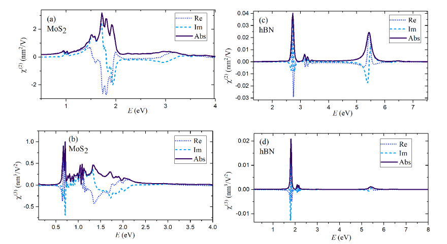
Figure 6: (a-b) Second- and third-harmonic susceptibilities of MoS₂. (d-e) Likewise, for hBN. Even though, we plot the susceptibilities in the extended frequency ranges shown in each panel for reference, recall that the underlying band structures are truncated; this limits the reliable ranges of validity of $\chi^{(2)}$ ($\chi^{(3)}$) to $\hbar\omega\lesssim 1.75\,(1.17)$ eV for MoS₂ and $\hbar\omega\lesssim 4.5\,(3.0)$ eV for hBN. [For MoS₂: $N^{2}_{k}=36^{2}$, $N_{c}=6$, $N_{v}=2$, $E_{0}=0.01$ V/Å, $\tau=0.05$ fs, $T=208$ fs, $\hbar\gamma=0.05$ eV. For hBN: $N^{2}_{k}=60^{2}$, $N_{c}=N_{v}=1$, $E_{0}=5\times 10^{-4}$ V/Å $(\chi^{(2)})$, $E_{0}=1\times 10^{-2}$ V/Å $(\chi^{(3)})$, $\tau=0.0125$ fs, $T=208$ fs, $\hbar\gamma=0.1$ eV.]

Having taken these aspects into account, we obtained the converged results shown in Fig. 6 for the second- and third-harmonic susceptibilities of MoS₂ and hBN. [For reference, we display the corresponding results without Coulomb interaction in Fig. 9]. In each case, the features we obtained here for the SH susceptibility with explicit account of interactions compare well with other recent calculations. For MoS₂, we obtain SH magnitudes of $|\chi^{(2)}(\hbar\omega=0.9)|\simeq 0.4$ nm²/V (A/B exciton features) and $|\chi^{(2)}(\hbar\omega=1.5)|\simeq 1.5$ nm²/V (C exciton feature). The former compare well with the corresponding values $\simeq 0.12$ and $\simeq 1.0$ obtained by Trolle et al.Trolle et al. (2014) using a parameterized TB model to solve the BSE; the latter tally with the value $\simeq 0.7$ nm²/V ($2.6\times 10^{-6}\,\text{esu}$) obtained ab initio by Grüning et al. Grüning and Attaccalite (2014b) at the C-exciton peak. Experimentally, Li et al.Li et al. (2013) reported $|\chi^{(2)}(\hbar\omega=1.53)|=8.8\times 10^{-31}$ mC/V² $\simeq 0.1$ nm²/V, while Woodward et al. Woodward et al. (2017) extracted $|\chi^{(2)}|=0.02$ nm²/V and $|\chi^{(3)}|=0.17$ nm³/V² from harmonic generation in MoS₂ under a laser field with $\omega_{0}\simeq 0.8$ eV (1560 nm). Our results in Fig. 6 for MoS₂ yield $|\chi^{(2)}(\hbar\omega=0.8)|\simeq 0.24$ nm²/V and $|\chi^{(3)}(\hbar\omega=0.8)|\simeq 0.25$ nm³/V². We consider them to be in reasonable agreement with experiments even though such comparisons are delicate because of a large dispersion in the magnitudes reported experimentally for high harmonic susceptibilities.

In relation to hBN, the first remark is that, even though our TB model contains only 2 bands and we consider only inter-band matrix elements of the dipole operator, we capture a clearly finite $\chi^{(2)}(\omega)$ with all the excitonic features previously observed in ab initio calculations Wirtz et al. (2006); Arnaud et al. (2006); Wirtz et al. (2008); Marini (2008); Attaccalite et al. (2011a, b); Yan et al. (2012); Grüning and Attaccalite (2014a); Cudazzo et al. (2016); Galvani et al. (2016); Koskelo et al. (2017); Ferreira et al. (2019); Attaccalite et al. (2018), as well as in perturbative calculations based on parameterized TB models Pedersen (2015). Our magnitudes, on the other hand, appear to be underestimated in comparison with these previous calculations by roughly one order of magnitude. For example, while the magnitude of our $\chi^{(2)}(\omega)$ in Fig. 6(c) is $\simeq 0.04$ nm²/V at its strongest peak ($\hbar\omega\simeq 1.7$ eV), the same peak has been reported with an intensity $\sim 0.2$ nm²/V, in both ab initio Grüning and Attaccalite (2014b); Wang et al. (2015); Lucking et al. (2018) and parameterized Pedersen (2015) calculations. We address this discrepancy in the next section, but we point out that the only experimental report we are aware of quotes Li et al. (2013) $|\chi^{(2)}(\hbar\omega=1.53)|=3\times 10^{-32}$ mC/V${}^{2}\simeq 0.003$ nm²/V.

In relation to calculations accounting for excitonic effects beyond second order, we are only aware of those by Attaccalite et al.Attaccalite et al. (2018) who calculate the frequency-dependent susceptibility for two-photon absorption in hBN. Unfortunately, that corresponds to the response function $\chi^{(3)}(\omega;\omega,\omega,-\omega)$ and not the third-harmonic $\chi^{(3)}(3\omega;\omega,\omega,\omega)$ that we can compute with our current implementation.

IV Discussion

Trade-offs in the time domain — Two key practical advantages of a time-domain formulation are: (i) Eq. (8) condenses the problem in a formally simple expression which is suitable for a general-purpose implementation; (ii) it entirely circumvents the explicit calculation of each order of a perturbative expansion on the strength of the external field. Even though expressions have been given for some nonlinear susceptibilities, for both independent Armstrong et al. (1962); Sipe and Ghahramani (1993); Aversa and Sipe (1995) and interacting Leitsmann et al. (2005) electrons, the terms contributing to each order quickly proliferate and become cumbersome to handle already at the second order, especially when they incorporate excitons Leitsmann et al. (2005). Besides, the actual calculation of each order inevitably demands a numerical integration over the BZ, even when using the simplest underlying Hamiltonians Pedersen (2015); Hipolito et al. (2016). Convergence of such integrations can become numerically challenging due to the presence of singularities in the spectral representation of the perturbative series that must be integrated.

On the other hand, the main trade-offs of a time-domain approach are: (i) the need of a post-processing stage that must be adapted to the information one desires to extract from the polarization (Fourier analysis, deconvolution, etc.); (ii) the total duration of $P(t)$ that must be acquired if one is interested in nonlinearities of very high order, or to achieve very high energy resolution in the final result. The issue here is that each time step in the numerical integration of Eq. (8) is costly because the electronic self-energy is non-diagonal in crystal momentum $\bm{k}$. In this regard, the strategy described in Section III.4 to obtain $\chi^{(n)}(\omega)$ is one of the worst case scenarios since it requires launching one wave for each frequency $\omega$ of interest. [The results in Figs. 3 and 6 required integrating the equation of motion (30) hundreds of times, given the frequency interval and resolution we sought.] Yet, using parameterized Hamiltonians and interactions makes such computation entirely feasible without extreme computational resources, while a fully ab initio implementation faces stringent computational challenges.

Ultrafast optical processes — This is where the current framework has a distinctive advantage: as the temporal profile of the exciting field can be arbitrary, this approach is best suited for realistic simulations of properties that are intrinsic of the time domain. These include simulating the response to pulsed excitation, response to purposefully tailored light pulses, or pump-probe scenarios. More interesting is the potential to simulate electronic processes at ultrafast timescales (e.g., femtoseconds) while natively accounting for electronic interactions; this will be possible by adequate extensions of the electronic self-energy to capture specific mechanisms of electronic relaxation (e.g., electron-phonon and electron-electron collisions). Finally, since this framework is non-perturbative in the external field and captures the evolution of the distribution function out of equilibrium, it is also naturally suited to characterize absorption saturation and other combined nonlinear+nonequilibrium effects of interest for applications.

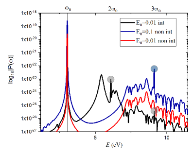
Figure 7: Frequency spectrum of $|P(\omega)|$ for hBN in response to a continuous monochromatic wave of frequency $\hbar\omega_{0}=3.04$ eV, showing results obtained with (“int”) and without (“no int”) Coulomb interaction. Note how, in the absence of interaction (blue and red curves), there is no second-harmonic response (no peak at $2\omega_{0}$), even when the field is strong enough to allow resolution of the third harmonic (blue curve). The shaded circles highlight the amplitude of the harmonic peaks at $\omega=n\omega_{0}$. [$N^{2}_{k}=60^{2}$, $N_{c}=N_{v}=1$, $\tau=0.0125$ fs, $T=208$ fs, $\hbar\gamma=0.1$ eV]

Intra-band transitions — As described in Section II.3, we approximated the diagonal matrix elements of the dipole operator as $\text{$\bm{r}$}_{mm\text{$\bm{k}$}}\simeq 0$, effectively assuming that only inter-band elements contribute to the optical response. Though this would be formally correct in linear response for a semiconductor at $T=0$ K, the importance of the intra-band contributions (IBCs) at higher orders has been a long and delicate subject of discussion (especially because it touches subtle aspects related to the choice of gauge and approximations to represent the coupling to the external electromagnetic field in the Hamiltonian Genkin and Mednis (1968); Aversa and Sipe (1995); Rza̧zewski and Boyd (2004); Taghizadeh et al. (2017); Ventura et al. (2017); Taghizadeh and Pedersen (2018)). A crucial disadvantage of this separation of contributions is that it breaks gauge invariance Földi (2017); Ernotte et al. (2018). The clearest and most striking example of the potential for inconsistencies arises in a two-band model: In the length-gauge and without interactions, equilibrium second-order perturbation theory predicts the vanishing of the second-order susceptibility in the ground state of a semiconductor, irrespective of the underlying symmetry Aversa and Sipe (1995); Hipolito et al. (2016). The reason is trivial: the $n$-th order response involves the product of $n+1$ matrix elements defining a chain of transitions that must return to the initial state, which is impossible if $n=2$ and only inter-band transitions are included. Recently, it has been shown that adding excitons to the perturbative quadratic susceptibilities does not change the conclusion: IBCs are necessary to obtain a finite quadratic response in a two-band model Pedersen (2015).

In contrast, our calculations yield a finite $\chi^{(2)}$ [Figs. 5 and 6(c)] for a two-band description of hBN without IBCs; moreover, the obtained $\chi^{(2)}$ has the frequency-dependent features seen in DFT+$GW$+BSE results Attaccalite et al. (2011a); Pedersen (2015). The fact we obtain a finite $\chi^{(2)}$ in a two-band description originates in the nonequilibrium nature of our approach. To appreciate that explicitly, consider Fig. 7 where we show $P(\omega)$ under a monochromatic field with frequency $\omega_{0}$, calculated with and without interactions. In line with the simple argument given above, the non-interacting traces have no SH response [no peak at $P(2\omega_{0})$], even when the field is strong enough to reveal a clear third-harmonic peak above the transient background [blue shaded disk; see also Fig. 9(c)]. In contrast, the interacting trace does show a clear peak at $\omega{\,=\,}2\omega_{0}$ (gray shaded disk), the magnitude of which defines the $\chi^{(2)}(\omega)$ plotted in Fig. 6(c) according to Eq. (28).

The conclusion in Ref. Pedersen, 2015 that IBCs are necessary to capture the SH susceptibility in a two-band model is conditioned by their underlying assumption of quasi-equilibrium: the populations on each band remain unchanged by the external field. (In our formulation, this assumption amounts to not evolving the self-energy away from its equilibrium value, which implies setting $\bm{\Sigma}_{\text{$\bm{k}$}}[G^{<}(t)]\to\bm{\Sigma}_{\text{$\bm{k}$}}[G^{<}(0)]$.) But one can see from Eqs. (4) and (5) of the cited reference that, by relaxing that assumption and explicitly integrating in time both coherences and populations, one obtains additional contributions to the second-order response that involve only inter-band matrix elements. This is not surprising because one reason for the absence of purely inter-band contributions under the quasi-equilibrium assumption is the perfect Pauli blocking effect, which arises because the occupations $f_{m\text{$\bm{k}$}}$ remain either 1 or 0 in that approximation, but not fractional. It thus follows that, when calculating the nonlinear response in a two-band model, one must not only include IBCs but also explicitly take into account the system’s deviation from equilibrium.

Therefore, strictly speaking, both our SH susceptibility and that in Ref. Pedersen, 2015 for hBN are incomplete. As we highlighted above, although qualitatively identical, our calculated $\chi^{(2)}(\omega)$ is one order of magnitude below that reported in Ref. Pedersen, 2015; moreover, the latter tallies with the ab initio result in Ref. Grüning and Attaccalite, 2014a that employs yet another methodology. This can be an indication that, though not a negligible contribution, the deviation from equilibrium might be less dominant than the effect of IBCs. In our framework, a definitive conclusion requires restoring the intra-band matrix elements into the perturbation term (11), which is beyond the scope of the present paper.

Numerical efficiency — The numerical scaling of this framework is extremely simple and follows directly from the nature of the problem defined by the equation of motion (8), the workhorse of the methodology. To integrate $P(t)$ in response to a single external wave or pulse requires a total of $T/\Delta t=L$ time steps; when a Runge-Kutta algorithm is employed, one must recall that advancing one time step requires a number of intermediate evaluations that will be discarded, with more discarded the higher the order Abramowitz and Stegun (1964). (Our current implementation can indeed be sped up by a factor of two by switching to an integration rule that reuses all evaluations in subsequent steps.) As for storage requirements, it is desirable, for expediency, to store the Coulomb matrix elements (17) which, being the only nondiagonal matrix in $\bm{k}$, is what ultimately determines the storage needs. Since its linear dimension is $N_{\text{tot}}=N_{k}^{2}(N_{c}+N_{v})^{2}$, it ultimately imposes a compromise between the number of points $N_{k}^{2}$ used to sample the BZ and the number of bands. But, as exemplified by our results in the one-wave-per-frequency (worst-case) scenario discussed in Section III.4, we were able to include up to $N_{c}+N_{v}=8$ bands and $N_{k}^{2}\sim 36^{2}\text{--}40^{2}$ to describe MoS₂ still within reasonable computational resources. Finally, the calculation time per integration step scales $\propto N_{\text{tot}}^{2}$ because the evaluation of the right-hand side of Eq. (8) can be coded as a matrix-vector product; this is explicitly shown in Fig. 8.

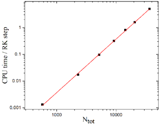
Figure 8: Typical scaling of the CPU seconds per integration time-step with the linear dimension of the Coulomb matrix, $N_{\text{tot}}=N_{k}^{2}(N_{c}+N_{v})^{2}$. The line is $\propto N_{\text{tot}}^{2}$.

V Conclusion

We have explicitly demonstrated that parameterized models are capable of retaining excellent agreement with experimental and ab-initio optical spectra over large frequency ranges, while significantly alleviating the computational demands of the time-domain framework proposed by Attaccalite et al.Attaccalite et al. (2011a) to study the response to arbitrary light fields. Therefore, our results broaden the practical reach of this general-purpose and versatile technique where multiple interacting and/or relaxation mechanisms can be incorporated in a systematic way, and which is natively suited to simulate the current frontier of ultrafast spectroscopy in solid-state materials. We have exposed in detail the relevant adaptations of the technique necessary for that, which will be of value to pursue further refinements and applications such as wave mixing or pump-probe simulations. Finally, we trust this will be a useful contribution to the current interest in robust general methods to tackle the combined nonlinear-nonequilibrium response of crystals under strong fields.

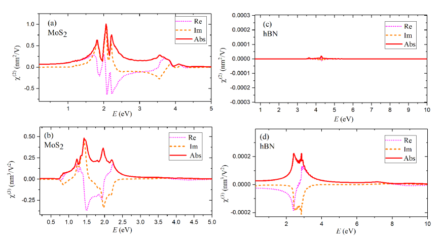
Figure 9: (a-b) Second- and third-harmonic susceptibilities of MoS₂ deliberately without Coulomb interactions. (d-e) Likewise, for hBN. Note how in (c) $\chi^{(2)}$ is within our noise floor (as expected for a non-interacting two-band model), in contrast with the interacting result shown in Fig. 6(c). [For MoS₂: $N^{2}_{k}=36^{2}$, $N_{c}=6$, $N_{v}=2$, $E_{0}=0.01$ V/Å $(\chi^{(2)})$, $E_{0}=0.05$ V/Å $(\chi^{(3)})$, $\tau=0.05$ fs, $T=208$ fs, $\hbar\gamma=0.05$ eV. For hBN $N^{2}_{k}=60^{2}$, $N_{c}=N_{v}=1$, $E_{0}=0.05$ V/Å, $\tau=0.0125$ fs, $T=208$ fs, $\hbar\gamma=0.1$ eV.]

References

- Boyd (2008) R. W. Boyd, Nonlinear Optics, 3rd ed. (Academic Press, Burlington, MA, 2008).
- Luppi and Véniard (2016) E. Luppi and V. Véniard, Semicond. Sci. Technol. 31, 123002 (2016).
- Wang et al. (2012) Q. H. Wang, K. Kalantar-Zadeh, A. Kis, J. N. Coleman, and M. S. Strano, Nat. Nanotechnol. 7, 699 (2012).
- Xia et al. (2014) F. Xia, H. Wang, D. Xiao, M. Dubey, and A. Ramasubramaniam, Nat. Photonics 8, 899 (2014).
- Wang et al. (2018) G. Wang, A. Chernikov, M. M. Glazov, T. F. Heinz, X. Marie, T. Amand, and B. Urbaszek, Rev. Mod. Phys. 90, 021001 (2018).
- Xu et al. (2014) X. Xu, W. Yao, D. Xiao, and T. F. Heinz, Nat. Phys. 10, 343 (2014).
- Schaibley et al. (2016) J. R. Schaibley, H. Yu, G. Clark, P. Rivera, J. S. Ross, K. L. Seyler, W. Yao, and X. Xu, Nat. Rev. Mater. 1, 16055 (2016).
- Cudazzo et al. (2011) P. Cudazzo, I. V. Tokatly, and A. Rubio, Phys. Rev. B 84, 085406 (2011).
- Thygesen (2017) K. S. Thygesen, 2D Mater. 4, 022004 (2017).
- Kotov et al. (2012) V. N. Kotov, B. Uchoa, V. M. Pereira, F. Guinea, and A. H. Castro Neto, Rev. Mod. Phys. 84, 1067 (2012).
- Ridolfi et al. (2018) E. Ridolfi, C. H. Lewenkopf, and V. M. Pereira, Phys. Rev. B 97, 205409 (2018).
- Liu et al. (2016) H. Liu, Y. Li, Y. S. You, S. Ghimire, T. F. Heinz, and D. A. Reis, Nat. Phys. 13, 262 (2016).
- Huber et al. (2001) R. Huber, F. Tauser, A. Brodschelm, M. Bichler, G. Abstreiter, and A. Leitenstorfer, Nature 414, 286 (2001).
- Kampfrath et al. (2013) T. Kampfrath, K. Tanaka, and K. A. Nelson, Nat. Photonics 7, 680 (2013).
- Kim et al. (2014) J. Kim, X. Hong, C. Jin, S.-F. F. Shi, C.-Y. Y. S. Chang, M.-H. H. Chiu, L.-J. J. Li, and F. Wang, Science 346, 1205 (2014).
- Hao et al. (2016) K. Hao, G. Moody, F. Wu, C. K. Dass, L. Xu, C. H. Chen, L. Sun, M. Y. Li, L. J. Li, A. H. MacDonald, and X. Li, Nat. Phys. 12, 677 (2016).
- Ye et al. (2017) Z. Ye, D. Sun, and T. F. Heinz, Nat. Phys. 13, 26 (2017).
- Onida et al. (2002) G. Onida, L. Reining, and A. Rubio, Rev. Mod. Phys. 74, 601 (2002).
- Chang et al. (2001) E. K. Chang, E. L. Shirley, and Z. H. Levine, Phys. Rev. B 65, 035205 (2001).
- Leitsmann et al. (2005) R. Leitsmann, W. G. Schmidt, P. H. Hahn, and F. Bechstedt, Phys. Rev. B 71, 195209 (2005).
- Aversa and Sipe (1995) C. Aversa and J. E. Sipe, Phys. Rev. B 52, 14636 (1995).
- Pedersen (2015) T. G. Pedersen, Phys. Rev. B 92, 235432 (2015).
- Souza et al. (2004) I. Souza, J. Iniguez, and D. Vanderbilt, Phys. Rev. B 69, 085106 (2004).
- Takimoto et al. (2007) Y. Takimoto, F. Vila, and J. Rehr, The Journal of Chem. Phys. 127, 154114 (2007).
- Ding et al. (2013) F. Ding, B. E. V. Kuiken, B. E. Eichinger, and X. Li, The Journal of Chem. Phys. 138, 064104 (2013).
- Pal et al. (2011) G. Pal, Y. Pavlyukh, W. Hübner, and H. Schneider, Eur. Phys. J. B 79, 327 (2011).
- Perfetto et al. (2015) E. Perfetto, D. Sangalli, A. Marini, and G. Stefanucci, Phys. Rev. B 92, 205304 (2015).
- Attaccalite et al. (2011a) C. Attaccalite, M. Grüning, and A. Marini, Phys. Rev. B 84, 245110 (2011a).
- Attaccalite and Grüning (2013) C. Attaccalite and M. Grüning, Phys. Rev. B 88, 235113 (2013).
- Grüning and Attaccalite (2014a) M. Grüning and C. Attaccalite, Phys. Rev. B 89, 081102(R) (2014a).
- Grüning et al. (2016) M. Grüning, D. Sangalli, and C. Attaccalite, Phys. Rev. B 94, 035149 (2016).
- Tancogne-Dejean et al. (2016) N. Tancogne-Dejean, C. Giorgetti, and V. Véniard, Phys. Rev. B 94, 125301 (2016).
- Hüser et al. (2013) F. Hüser, T. Olsen, and K. S. Thygesen, Phys. Rev. B - Condens. Matter Mater. Phys. 88, 245309 (2013).
- Qiu et al. (2013) D. Y. Qiu, F. H. da Jornada, and S. G. Louie, Phys. Rev. Lett. 111, 216805 (2013).
- Qiu et al. (2015) D. Y. Qiu, F. H. da Jornada, and S. G. Louie, Phys. Rev. Lett. 115, 119901(E) (2015).
- Jain et al. (2013) A. Jain, S. P. Ong, G. Hautier, W. Chen, W. D. Richards, S. Dacek, S. Cholia, D. Gunter, D. Skinner, G. Ceder, and K. A. Persson, APL Mater. 1, 011002 (2013).
- Saal et al. (2013) J. E. Saal, S. Kirklin, M. Aykol, B. Meredig, and C. Wolverton, JOM 65, 1501 (2013).
- Rasmussen and Thygesen (2015) F. A. Rasmussen and K. S. Thygesen, J. Phys. Chem. C 119, 13169 (2015).
- Mounet et al. (2018) N. Mounet, M. Gibertini, P. Schwaller, D. Campi, A. Merkys, A. Marrazzo, T. Sohier, I. E. Castelli, A. Cepellotti, G. Pizzi, and N. Marzari, Nat. Nanotechnol. 13, 246 (2018).
- Zhou et al. (2019) J. Zhou, L. Shen, M. D. Costa, K. A. Persson, S. P. Ong, P. Huck, Y. Lu, X. Ma, Y. Chen, H. Tang, and Y. P. Feng, Sci. Data 6, 86 (2019).
- Trolle et al. (2014) M. L. Trolle, G. Seifert, and T. G. Pedersen, Phys. Rev. B 89, 235410 (2014).
- Wu et al. (2015a) F. Wu, F. Qu, and A. H. MacDonald, Phys. Rev. B 91, 075310 (2015a).
- Slater and Koster (1954) J. C. Slater and G. F. Koster, Phys. Rev. 94, 1498 (1954).
- Ridolfi et al. (2015) E. Ridolfi, D. Le, T. S. Rahman, E. R. Mucciolo, and C. H. Lewenkopf, J. Phys.: Condens. Matter 27, 365501 (2015).
- Galvani et al. (2016) T. Galvani, F. Paleari, H. P. C. Miranda, A. Molina-Sanchez, L. Wirtz, S. Latil, H. Amara, and F. Ducastelle, Phys. Rev. B 94, 125303 (2016).
- Schmitt-Rink et al. (1988) S. Schmitt-Rink, D. S. Chemla, and H. Haug, Phys. Rev. B 37, 941 (1988).
- Note (1) That is frequently the case for 2D semiconductors; see for example Refs. \rev@citealpnumHuser2013, Qiu2013, Qiu2015-erratum.
- Resta (1994) R. Resta, Rev. of Modern Phys. 66, 899 (1994).
- Kadanoff and Baym (1962) L. P. Kadanoff and G. Baym, Quantum statistical mechanics: Green’s function methods in equilibrium and nonequilibrium problems (W. A. Benjamin, New York, 1962).
- Kremp et al. (2005) D. Kremp, M. Schlanges, and W.-D. Kraeft, Quantum Statistics of Nonideal Plasmas (Springer-Verlag, Berlin/Heidelberg, 2005).
- Keldysh (1964) L. Keldysh, Sov. Phys. JETP 20, 1018 (1964).
- Schäfer and Wegener (2002) W. Schäfer and M. Wegener, Semiconductor Optics and Transport Phenomena, 5th ed., Advanced Texts in Physics, Vol. 13 (Springer Berlin Heidelberg, Berlin, Heidelberg, 2002) p. 1652.
- Hybertsen and Louie (1986) M. S. Hybertsen and S. G. Louie, Phys. Rev. B 34, 5390 (1986).
- Hedin and Lundqvist (1970) L. Hedin and S. Lundqvist, Solid State Physics 23, 1 (1970).
- Becke (1993) A. D. Becke, J. Chem. Phys. 98, 5648 (1993).
- Ventura et al. (2019) G. B. Ventura, D. Passos, J. M. Viana Parente Lopes, and J. M. B. Lopes dos Santos, J. Phys. Condens. Matter 32, 185701 (2019).
- Note (2) Should two bands cross and at localized points, our implementation explicitly removes the divergence by setting at such .
- Pedersen et al. (2001) T. G. Pedersen, K. Pedersen, and T. B. Kriestensen, Phys. Rev. B 63, 201101(R) (2001).
- Hedin (1965) L. Hedin, Phys. Rev. 139, A796 (1965).
- Bruneval et al. (2006) F. Bruneval, N. Vast, and L. Reining, Phys. Rev. B 74, 045102 (2006).
- Rohlfing and Louie (2000) M. Rohlfing and S. G. Louie, Phys. Rev. B 62, 4927 (2000).
- Schöne and Ekardt (2002) W.-D. Schöne and W. Ekardt, Phys. Rev. B 65, 113112 (2002).
- Marini and Del Sole (2003) A. Marini and R. Del Sole, Phys. Rev. Lett. 91, 176402 (2003).
- Trevisanutto and Vignale (2016) P. E. Trevisanutto and G. Vignale, The Journal of Chemical Physics 144, 204122 (2016).
- Note (3) To handle the -diagonal cases where , we use the regularization scheme adopted in Ref. \rev@citealpnumRidolfi2018.
- Keldysh (1979) L. V. Keldysh, JETP Lett. 29, 658 (1979).
- Trolle et al. (2017) M. L. Trolle, T. G. Pedersen, and V. Véniard, Scientific Reports 7, 39844 (2017).
- Chernikov et al. (2014) A. Chernikov, T. C. Berkelbach, H. M. Hill, A. Rigosi, Y. Li, O. B. Aslan, D. R. Reichman, M. S. Hybertsen, and T. F. Heinz, Phys. Rev. Lett. 113, 076802 (2014).
- Rodin et al. (2014) A. S. Rodin, A. Carvalho, and A. H. Castro Neto, Phys. Rev. B 90, 075429 (2014).
- Note (4) To fix the relative phases in the numerical diagonalization of the Bloch Hamiltonian for different , we require to be real, as suggested in Ref. \rev@citealpnumRohlfing2000 and previously implemented in Ref. \rev@citealpnumRidolfi2018.
- Wismer and Yakovlev (2018) M. S. Wismer and V. S. Yakovlev, Phys. Rev. B 97, 144302 (2018).
- M. Galassi et al. (2009) M. Galassi et al., GNU Scientific Library: Reference Manual, 3rd ed. (Network Theory, 2009).
- Note (5) Since the linear dimension of the problem is very large in virtually all cases of interest, there is no advantage in using higher-order methods which are only efficient when the function evaluations required to advance each time step are fast, which is not the case here.
- Orfanidis (1996) S. J. Orfanidis, Introduction to Signal Processing (Prentice Hall, 1996).
- Li et al. (2014) Y. Li, A. Chernikov, X. Zhang, A. Rigosi, H. M. Hill, A. M. van der Zande, D. A. Chenet, E.-M. Shih, J. Hone, and T. F. Heinz, Phys. Rev. B 90, 205422 (2014).
- Jayaswal et al. (2018) G. Jayaswal, Z. Dai, X. Zhang, M. Bagnarol, A. Martucci, and M. Merano, Opt. Lett. 43, 703 (2018).
- Klots et al. (2014) A. R. Klots, A. K. M. Newaz, B. Wang, D. Prasai, H. Krzyzanowska, J. Lin, D. Caudel, N. J. Ghimire, J. Yan, B. L. Ivano, K. A. Velizhanin, A. Burger, D. G. Mandru, N. H. Tolk, S. T. Pantelides, and K. I. Bolotin, Sci. Rep. 4, 6608 (2014).
- Molina-Sánchez et al. (2015) A. Molina-Sánchez, K. Hummer, and L. Wirtz, Surf. Sci. Rep. 70, 554 (2015).
- Xiao et al. (2012) D. Xiao, G.-B. Liu, W. Feng, X. Xu, and W. Yao, Phys. Rev. Lett. 108, 196802 (2012).
- Mak et al. (2012) K. F. Mak, K. He, J. Shan, and T. F. Heinz, Nat. Nanotechnol. 7, 494 (2012).
- Zeng et al. (2012) H. Zeng, J. Dai, W. Yao, D. Xiao, and X. Cui, Nat. Nanotechnol. 7, 490 (2012).
- Arnaud et al. (2006) B. Arnaud, S. Lebègue, P. Rabiller, and M. Alouani, Phys. Rev. Lett. 96, 026402 (2006).
- Zhang et al. (2014) C. Zhang, A. Johnson, C.-L. Hsu, L.-J. Li, and C.-K. Shih, Nano Lett. 14, 2443 (2014).
- Mak et al. (2010) K. F. Mak, C. Lee, J. Hone, J. Shan, and T. F. Heinz, Phys. Rev. Lett. 105, 136805 (2010).
- Zhang et al. (2013) Y. Zhang, T.-R. Chang, B. Zhou, Y.-T. Cui, H. Yan, Z. Liu, F. Schmitt, J. Lee, R. Moore, Y. Chen, H. Lin, H.-T. Jeng, S.-K. Mo, Z. Hussain, A. Bansil, and Z.-X. Shen, Nat. Nanotechnol. 9, 111 (2013).
- Zhu et al. (2015) B. Zhu, X. Chen, and X. Cui, Sci. Rep. 5, 9218 (2015).
- Malard et al. (2013) L. M. Malard, T. V. Alencar, A. M. Barboza, K. F. Mak, and A. M. de Paula, Phys. Rev. B 87, 201401(R) (2013).
- Kumar et al. (2013) N. Kumar, S. Najmaei, Q. Cui, F. Ceballos, P. M. Ajayan, J. Lou, and H. Zhao, Phys. Rev. B 87, 161403(R) (2013).
- Trolle et al. (2015) M. L. Trolle, Y.-C. Tsao, K. Pedersen, and T. G. Pedersen, Phys. Rev. B 92, 161409(R) (2015).
- Glazov et al. (2017) M. M. Glazov, L. E. Golub, G. Wang, X. Marie, T. Amand, and B. Urbaszek, Phys. Rev. B 95, 035311 (2017).
- Soh et al. (2018) D. B. S. Soh, C. Rogers, D. J. Gray, E. Chatterjee, and H. Mabuchi, Phys. Rev. B 97, 165111 (2018).
- Mamy et al. (1981) R. Mamy, J. Thomas, G. Jezequel, and J. Lemonnier, J. Physique Lett. 42, 473 (1981).
- Watanabe et al. (2004) K. Watanabe, T. Taniguchi, and H. Kanda, Nat. Mater. 3, 404 (2004).
- Song et al. (2010) L. Song, L. Ci, H. Lu, P. B. Sorokin, C. Jin, J. Ni, A. G. Kvashnin, D. G. Kvashnin, J. Lou, B. I. Yakobson, and P. M. Ajayan, Nano Letters 10, 3209 (2010).
- Kim et al. (2012) K. K. Kim, A. Hsu, X. Jia, S. M. Kim, Y. Shi, M. Hofmann, D. Nezich, J. F. Rodriguez-Nieva, M. Dresselhaus, T. Palacios, and J. Kong, Nano Letters 12, 161 (2012).
- Wu et al. (2015b) Q. Wu, J.-H. Park, S. Park, S. J. Jung, H. Suh, N. Park, W. Wongwiriyapan, S. Lee, Y. H. Lee, and Y. J. Song, Scientific Reports 5, 16159 (2015b).
- Wirtz et al. (2006) L. Wirtz, A. Marini, and A. Rubio, Phys. Rev. Letters 96, 126104 (2006).
- Wirtz et al. (2008) L. Wirtz, A. Marini, M. Grüning, C. Attaccalite, G. Kresse, and A. Rubio, Phys. Rev. Lett. 100, 189701 (2008).
- Marini (2008) A. Marini, Phys. Rev. Letters 101, 106405 (2008).
- Attaccalite et al. (2011b) C. Attaccalite, M. Bockstedte, A. Marini, A. Rubio, and L. Wirtz, Phys. Rev. B 83, 144115 (2011b).
- Yan et al. (2012) J. Yan, K. W. Jacobsen, and K. S. Thygesen, Phys. Rev. B 86, 045208 (2012).
- Cudazzo et al. (2016) P. Cudazzo, L. Sponza, C. Giorgetti, L. Reining, F. Sottile, and M. Gatti, Phys. Rev. Lett. 116, 066803 (2016).
- Koskelo et al. (2017) J. Koskelo, G. Fugallo, M. Hakala, M. Gatti, F. Sottile, and P. Cudazzo, Phys. Rev. B 95, 035125 (2017).
- Ferreira et al. (2019) F. Ferreira, A. J. Chaves, N. M. R. Peres, and R. M. Ribeiro, J. Opt. Soc. Am. B 36, 674 (2019).
- Attaccalite et al. (2018) C. Attaccalite, M. Grüning, H. Amara, S. Latil, and F. Ducastelle, Phys. Rev. B 98, 165126 (2018).
- Chiu et al. (2015) M.-H. Chiu, C. Zhang, H.-W. Shiu, C.-P. Chuu, C.-H. Chen, C.-Y. S. Chang, C.-H. Chen, M.-Y. Chou, C.-K. Shih, and L.-J. Li, Nat. Commun. 6, 7666 (2015).
- Note (6) This has the same practical effect as, for example, adiabatically turning the field on over a time , instead of a sudden turn-on.
- Note (7) For pedagogic purposes, we note that this is the same phenomenon that frequently happens experimentally, where one might need to acquire a week signal for times long enough to bring it above the noise floor. The fact that the background tails correspond to the transient component of the signal, as highlighted in Fig. 5, is confirmed by the fact that they scale as can be inspected in that figure.
- Note (8) A loose way of illustrating the physical content of this statement is to think of a classical oscillator driven at the resonant frequency: Although its amplitude begins growing, upon waiting long enough one eventually sees that it does not diverge (strict resonance), reaching instead a finite maximum determined by the damping constant.
- Grüning and Attaccalite (2014b) M. Grüning and C. Attaccalite, Phys. Rev. B 90, 199901(E) (2014b).
- Li et al. (2013) Y. Li, Y. Rao, K. F. Mak, Y. You, S. Wang, C. R. Dean, and T. F. Heinz, Nano Lett. 13, 3329 (2013).
- Woodward et al. (2017) R. I. Woodward, R. T. Murray, C. F. Phelan, R. E. P. de Oliveira, T. H. Runcorn, E. J. R. Kelleher, S. Li, E. C. de Oliveira, G. J. M. Fechine, G. Eda, and C. J. S. de Matos, 2D Mater. 4, 011006 (2017).
- Note (9) Perhaps not surprisingly since these frequencies lie near resonant features of the susceptibilities and, as a result, the magnitude of the response varies noticeably under small deviations from those resonances. Small deviations can appear routinely due, for example, to sample variability, different pulse shape or duration, the use of different substrates, lack of temperature control, and thermal effects due to exposure to highly energetic laser beam.
- Wang et al. (2015) F. Wang, Z. Wang, Q. Wang, F. Wang, L. Yin, K. Xu, Y. Huang, and J. He, Nanotechnology 26, 292001 (2015).
- Lucking et al. (2018) M. C. Lucking, K. Beach, and H.Terrones, Scientific Reports 8, 10118 (2018).
- Armstrong et al. (1962) J. A. Armstrong, N. Bloembergen, J. Ducuing, and P. S. Pershan, Phys. Rev. 127, 1918 (1962).
- Sipe and Ghahramani (1993) J. E. Sipe and E. Ghahramani, Phys. Rev. B 48, 11705 (1993).
- Hipolito et al. (2016) F. Hipolito, T. G. Pedersen, and V. M. Pereira, Phys. Rev. B 94, 045434 (2016).
- Note (10) For example, while the one-wave-per-frequency approach was employed in Ref. \rev@citealpnumAttaccalite2011 to study the nonequilibrium band populations, it could only analyze a select (two) frequencies.
- Genkin and Mednis (1968) V. N. Genkin and P. M. Mednis, JETP 27, 609 (1968).
- Rza̧zewski and Boyd (2004) K. Rza̧zewski and R. W. Boyd, J. Mod. Opt. 51, 1137 (2004).
- Taghizadeh et al. (2017) A. Taghizadeh, F. Hipolito, and T. G. Pedersen, Phys. Rev. B 96, 195413 (2017).
- Ventura et al. (2017) G. B. Ventura, D. J. Passos, J. M. B. Lopes dos Santos, J. M. Viana Parente Lopes, and N. M. R. Peres, Phys. Rev. B 96, 035431 (2017).
- Taghizadeh and Pedersen (2018) A. Taghizadeh and T. G. Pedersen, Phys. Rev. B 97, 205432 (2018).
- Földi (2017) P. Földi, Phys. Rev. B 96, 035112 (2017).
- Ernotte et al. (2018) G. Ernotte, T. J. Hammond, and M. Taucer, Phys. Rev. B 98, 235202 (2018).
- Abramowitz and Stegun (1964) M. Abramowitz and I. A. Stegun, Handbook of Mathematical Functions (Dover, New York, 1964).