Stability of the coexistence phase of chiral superconductivity and noncollinear spin ordering… Stability of the coexistence phase of chiral superconductivity and noncollinear spin ordering with a nontrivial topology and strong electron correlations V. V. Val’kov, A. O. Zlotnikov Val’kov V. V., Zlotnikov A. O. 05.03.201919.04.2019

Stability of the coexistence phase of chiral superconductivity and noncollinear spin ordering with a nontrivial topology and strong electron correlations

Abstract

We show that the quantum charge and spin fluctuations, while sufficiently renormalizing the magnetic order parameter, do not destroy the coexistence phase of chiral $d+id$ superconductivity and $120^{\circ}$ spin ordering in a strongly correlated 2D system with a triangular lattice. The nontrivial topology characterized by the topological invariant $\tilde{N}_{3}$ is also preserved. It is shown that the Majorana mode exist among edge states in the topologically nontrivial phase. The spatial structure of such mode is determined. The spin and charge fluctuations shift the critical values of electron density at which quantum topological transitions occur. Increasing intersite Coulomb repulsion leads to decrease in the number of the topological transitions.

1. Introduction

Recently, several superconducting systems have been proposed in which the formation of Majorana edge states is possible. Among them are, for example, superconductors with chiral p-wave symmetry [1, 2], interfaces of a superconductor and a topological insulator [3, 4], systems with spin-orbit interaction and proximity-induced superconductivity [5, 6, 7, 8, 9]. Experimentally, the greatest progress has been achieved for semiconductor nanowires InAs, InSb epitaxially coated by superconducting Al [10]. A quantized peak of the zero-bias conductance has been detected upon increasing an external magnetic field [10].

Recently it has been found that the Majorana modes can be implemented in materials with coexisting spin-singlet superconductivity and a long-range magnetic order [11, 12]. Such scenario is perspective due to the possibility of appearance of the Majorana modes in a condensed matter system, while there is no the spin-orbit interaction and an external magnetic field. In this framework the existence of the Majorana modes is demonstrated in superconducting systems with helical magnetic ordering (such as, for example, HoMo₆S₈, ErRh₄B₄) [11].

It is widely believed that, due to bulk-boundary correspondence, the edge and Majorana modes appear when the ground state of the system with periodic boundary conditions corresponds to a phase with nontrivial topology. The classification of such phases is carried out by using the topological invariant. In the simplest cases of 1D or 2D superconducting systems with broken time-reversal symmetry (symmetry class D [13]) described by quadratic Hamiltonians topological invariants are the $\mathbb{Z}_{2}$ invariant (Majorana number [2]) or $\mathbb{Z}$ invariant, respectively. A relation between two invariants is described in Ref. [14] for noncentrosymmetric superconductors. A transition between phases with different values of the topological invariant is implemented when the gap in the elementary excitation spectrum is closed [15].

Previously, it was predicted that the Majorana modes can be observed in 2D systems with a triangular lattice in the coexistence phase of chiral $d_{1}+id_{2}$ superconductivity and a stripe magnetic order [12]. However, the further analysis showed that chiral superconductivity does not coexist with stripe spin ordering, but coexists with a magnetic order corresponding to a $120^{\circ}$ structure [16]. The conditions for implementation of the Majorana modes in this coexistence phase are defined [17]. The $\mathbb{Z}_{2}$ and $\mathbb{Z}$ invariants are calculated for the quadratic Hamiltonian and it is shown that topologically nontrivial phases with an odd value of the $\mathbb{Z}$ invariant correspond to the parametric regions with the Majorana modes.

In the last time, the interest to the problem of electron correlations in topological phases has increased due to the fact that the correlations can lead to a change in the topological classification [18]. Although the classification is preserved for systems of even dimensions described by the $Z$-invariant [19] (for example, the symmetry class D such as the above mentioned systems with the triangular lattice).

The topological classification of systems with interaction can be based on a universal method, where the topological invariant is determined in terms of the Green functions [15]. For the 2D systems with the gapped excitation spectrum the $Z$-invariant is represented through the matrix Green function [20]. In [15], this invariant is denoted as $\tilde{N_{3}}$. Use of $\tilde{N_{3}}$ has allowed to demonstrate a nontrivial topology in quantum-Hall-effect systems [20], the phases of liquid helium ³He-A [21], ³He-B [22]. Recently, it has been shown [23] that the Green function at zero frequency can be used to describe topological phases.

The development of a topological classification method of strongly correlated materials with a triangular lattice in the coexistence phase of chiral superconductivity and noncollinear spin ordering is associated with the study of the stability of such phase a with regard to charge and spin fluctuations. It is related with the fact that, due to the reduced dimension and frustrated exchange interaction in the triangular lattice, the role of quantum fluctuations greatly increases in the mechanism of destruction of the ordered phase.

In this work, we show that the magnetic order parameter is strongly renormalized in the experimentally studied range of doping of sodium cobaltates. However, the structure of the spin ordering is preserved. For the coexistence phase of chiral superconductivity and 120^∘ spin structure the Green functions are obtained and the topological characteristics of this phase are determined using the invariant $\tilde{N_{3}}$. The change in the topological properties with increasing electron concentration and Coulomb repulsion is established. Namely, we identify a decrease in the number of topological transitions with increasing the Coulomb interaction parameter. Based on the solution of the equations for the Green functions with open boundary condition along one direction of the 2D lattice the spatial structure of the Majorana mode is demonstrated in the topologically nontrivial phase.

2. Model

To study the coexistence phase of chiral superconductivity and 120^∘ spin ordering with regard to spin-charge fluctuations and strong electron correlations we use $t-J-V$ model. For definiteness, we consider electron-doped systems such as the superconducting Na_xCoO₂ hydrate [24]. The Hamiltonian in the atomic representation is determined by the expression:

$$H = \sum_{f\sigma}\left(\varepsilon-\mu\right)X_{f}^{\sigma\sigma}+\sum_{f}\left(2\varepsilon+U-2\mu\right)X_{f}^{22}+$$ (1)

$$+ \sum_{fm\sigma}t_{fm}X_{f}^{2\bar{\sigma}}X_{m}^{\bar{\sigma}2}+\frac{V}{2}\sum_{f\delta}n_{f}n_{f+\delta}+$$

$$+ \sum_{fm}J_{fm}\left(X_{f}^{\uparrow\downarrow}X_{m}^{\downarrow\uparrow}-X_{f}^{\uparrow\uparrow}X_{m}^{\downarrow\downarrow}\right),$$

where $\varepsilon$ is the bare electron energy, $\mu$ is the chemical potential, $U$ is the on-site Coulomb repulsion parameter, $t_{fm}$ is the hopping parameter, $V$ denotes the inter-site Coulomb interaction parameter, $n_{f}=X_{f}^{\uparrow\uparrow}+X_{f}^{\downarrow\downarrow}+2X_{f}^{22}$ is the electron number operator at the site, and $J_{fm}$ is the exchange interaction parameter.

3. Gapless excitations in the coexistence phase

It is known [15] that the topological transitions occur when the elementary fermion excitations for the system with periodic boundary conditions become gapless. The excitation spectrum in the noncollinear magnetic phase is gapless on the Fermi contour (the line in the 2D Brillouin zone) at all levels of doping. In the superconducting phase with the chiral $d_{1}+id_{2}$ symmetry of the order parameter the gapless excitations are realized only at the specific points of the Brillouin zone (nodal points) with position depending on the electron density [25].

It is not difficult to establish the conditions for nodal excitations in the coexistence phase by analyzing the fermion spectrum [26]:

$$E_{1,2\,p} = \left[\frac{1}{2}\left(\xi_{p}^{2}+\xi_{p-Q}^{2}+|\Delta_{p}|^{2}+|\Delta_{-p+Q}|^{2}\right)\right.+$$ (2)

$$+ \left.R_{p}R_{p-Q}\mp\lambda_{p}\right]^{1/2},$$

where

$$\lambda_{p}=\left\{\frac{1}{4}\left(\xi_{p}^{2}-\xi_{p-Q}^{2}+|\Delta_{p}|^{2}-|\Delta_{-p+Q}|^{2}\right)^{2}+\right.$$

$$\left.+R_{p}R_{p-Q}\left[\left(\xi_{p}+\xi_{p-Q}\right)^{2}+|\Delta_{p}+\Delta_{-p+Q}|^{2}\right]\right\}^{1/2}.$$

The following notations are introduced $\xi_{p}=\varepsilon+U-\mu+J_{0}(1-n/2)+V_{0}n+nt_{p}/2=\xi_{0}+nt_{p}/2$, $n=\left\langle n_{f}\right\rangle$ is the on-site electron density, $J_{0}$, $J_{Q}$ are the Fourier transforms of the exchange interaction for the quasi-momentums $(0,0)$, ${\bf Q}$, $V_{0}=6V$, $R_{p}=M(t_{p}-J_{Q})$, $R_{p-Q}=M(t_{p-Q}-J_{Q})$, $M$ is the amplitude of the nonuniform magnetic order parameter determining the spin structure as $\left\langle{\bf S}_{f}\right\rangle=M\left(\cos({\bf Qf}),-\sin({\bf Qf}),0\right)$, $\Delta_{p}$ is the superconducting order parameter with the chiral $d_{1}+id_{2}$ and $p_{1}+ip_{2}$ invariants.

The nodal points of the spectrum (2) in the coexistence phase are determined by the equations:

$$\text{Im}\left(\Delta_{p}\Delta_{-p+Q}^{*}\right) = 0,$$ (3)

$$\left|\xi_{p}\Delta_{-p+Q}-\xi_{p-Q}\Delta_{p}\right| = 0,$$ (4)

$$R_{p}R_{p-Q}-\xi_{p}\xi_{p-Q}-\text{Re}\left(\Delta_{p}\Delta_{-p+Q}^{*}\right) = 0.$$ (5)

The spin 120^∘ ordering on the triangular lattice is defined by the vector ${\bf Q}=(2\pi/3,2\pi/3)$. Hereinafter coordinates of wave vectors are given in the basis of reciprocal lattice unit vectors. In this case, the equality $\Delta_{p}=\Delta_{-p+Q}=0$ satisfying Eqs. (3) and (4) holds at the center of the hexagonal Brillouin zone (point $\Gamma=(0,0)$) and at its boundaries (points $K=Q$, $K^{\prime}=-Q$). The parameters for the gapless excitations at the point $K^{\prime}$ are found from the equation:

$$M(n)=\left|\frac{-\tilde{\mu}(n,M)-3n/2(t_{1}-2t_{2}+t_{3})}{-3(t_{1}-2t_{2}+t_{3})+3(J_{1}-2J_{2})}\right|,$$ (6)

where $\tilde{\mu}(n,M)=\mu(n,M)-J_{0}(1-n/2)-V_{0}n$; $t_{1}$, $t_{2}$, $t_{3}$ are hopping parameters for three coordination spheres, $J_{1}$ and $J_{2}$ are the exchange parameters between nearest and next-nearest spins, respectively.

The excitation spectrum is gapless at the points $\Gamma$ and $K$ simultaneously if the following equation is satisfied:

$$M^{2}(n) - \left(\frac{-\tilde{\mu}(n,M)-3n/2(t_{1}-2t_{2}+t_{3})}{-3(t_{1}-2t_{2}+t_{3})+3(J_{1}-2J_{2})}\right)\times$$ (7)

$$\times\left(\frac{-\tilde{\mu}(n,M)+3n(t_{1}+t_{2}+t_{3})}{6(t_{1}+t_{2}+t_{3})+3(J_{1}-2J_{2})}\right)=0.$$

To find the exact conditions for development of the gapless spectrum of fermion quasiparticles, and hence the conditions for topological transitions with changing electron density it is necessary to obtain the expression for $M$ renormalized by spin and charge fluctuations. This problem is solved in the next section.

4. Renormalization of the magnetic amplitude $\bf{M}$

The theoretical description of magnets with the 120^∘ ordering of localized spins is carried out in [27, 28, 29, 30, 31]. The electronic ensemble on the triangular lattice is studied in the framework of the Hubbard model with mean-field [32] and slave-boson [33] approximations. The phase diagrams with different spin and charge orderings have been obtained. It is significant that the ground state with 120^∘ spin ordering is preserved upon doping near half filling. Using the Monte Carlo method, coexistence of superconductivity and 120^∘ spin ordering has been found near $n=1.1$ [34].

For simplicity of derivation of the renormalizing $M$ the unitary transformation of the Hamiltonian is made

$$H\to\tilde{H} = UHU^{{\dagger}},$$ (8)

$$U = \prod_{f}\left[\exp\left(i\frac{\pi}{2}S_{f}^{y}\right)\exp\left(i\theta_{f}S_{f}^{z}\right)\right],\,\,\,\theta_{f}=-{\bf Qf},$$

corresponding to the rotation of the coordinate frame such as the $z$ axis becomes aligned with $\left\langle{\bf S}_{f}\right\rangle$ at each site. The transformation rules for the operators are:

$$S_{f}^{x}\to\tilde{S}_{f}^{x} = \cos(\theta_{f})S_{f}^{z}-\sin(\theta_{f})S_{f}^{y},$$

$$S_{f}^{y}\to\tilde{S}_{f}^{y} = \cos(\theta_{f})S_{f}^{y}+\sin(\theta_{f})S_{f}^{z},$$

$$S_{f}^{z}\to\tilde{S}_{f}^{z} = -S_{f}^{x},$$

$$X_{f}^{\sigma\sigma}\to\tilde{X}_{f}^{\sigma\sigma} = \sum_{s=\uparrow,\downarrow}X_{f}^{ss}/2-\eta_{\sigma}\left(X_{f}^{\uparrow\downarrow}+X_{f}^{\downarrow\uparrow}\right)/2,$$

$$X_{f}^{\bar{\sigma}2}\to\tilde{X}_{f}^{\bar{\sigma}2}=\exp(i\eta_{\bar{\sigma}}\theta_{f}/2)\left(X_{f}^{\bar{\sigma}2}-\eta_{\bar{\sigma}}X_{f}^{\sigma 2}\right)/\sqrt{2},$$ (9)

where $X_{f}^{\uparrow\downarrow}=S_{f}^{x}+iS_{f}^{y}$, $\eta_{\sigma}=+1,\,-1$, for $\sigma=\uparrow,\,\downarrow$, respectively.

The transformed Hamiltonian with the obtained mean-field contributions has a form

$$\tilde{H} = \sum_{f\sigma}\tilde{\xi}_{\sigma}X_{f}^{\sigma\sigma}+\sum_{f}\left(2\varepsilon+U+2nV_{0}-2\mu\right)X_{f}^{22}+$$

$$+ \sum_{fm\sigma}t_{fm}\cos\frac{{\bf Q}}{2}\left({\bf f}-{\bf m}\right)X_{f}^{2\bar{\sigma}}X_{m}^{\bar{\sigma}2}-$$

$$- i\sum_{fm\sigma}t_{fm}\sin\frac{{\bf Q}}{2}\left({\bf f}-{\bf m}\right)X_{f}^{2\sigma}X_{m}^{\bar{\sigma}2}+$$

$$+ \sum_{fm}\frac{J_{fm}}{2}\left(1+\cos{\bf Q}\left({\bf f}-{\bf m}\right)\right)X_{f}^{\uparrow\downarrow}X_{m}^{\downarrow\uparrow}$$

$$+ \sum_{fm}\frac{J_{fm}}{4}\left(1-\cos{\bf Q}({\bf f}-{\bf m})\right)\left(X_{f}^{\uparrow\downarrow}X_{m}^{\uparrow\downarrow}+X_{f}^{\downarrow\uparrow}X_{m}^{\downarrow\uparrow}\right).$$

Only those terms describing the exchange interaction are taken into account that lead to fluctuation-induced corrections in the one-loop approximation. Here $\tilde{\xi}_{\sigma}=\varepsilon-\mu-(1-n/2)J_{0}+nV_{0}-\eta_{\sigma}h_{Q}$ and $h_{Q}=-MJ_{Q}$.

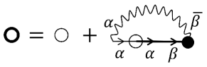
Figure 1: Fig. 1 Diagrams for $\left\langle X_{f}^{\uparrow\uparrow}\right\rangle$

Using the completeness condition of single-ion states and the definition connecting the electron concentration to filling numbers one can obtain the expression for the amplitude of the magnetic parameter order which is convenient to calculate: $M=n/2-1+N_{\uparrow}$. Here $N_{\uparrow}=\left\langle X_{f}^{\uparrow\uparrow}\right\rangle$ is the filling number of a state with a spin projection $1/2$. To find this number, the diagrammatic form of perturbation theory in the atomic representation is used. The diagrammatic representation for $N_{\uparrow}$ with regard to the first contributions caused by the spin and charge fluctuations is shown in Fig. 1. In the second diagram, $\alpha$ denotes the type of elementary excitation (root vector [35, 36]). For $\alpha=(\uparrow~{}\downarrow)$ this diagram determines contributions from spin fluctuations. In this case the second root vector takes two values $\beta=(\uparrow~{}\downarrow),~{}(\downarrow~{}\uparrow)$ [36, 37]. The charge fluctuations are described by two terms in accordance with the fact that the fermion root vector is $\alpha=(\uparrow~{}2)$ and $\beta$ takes two values $(\uparrow~{}2)$ and $(\downarrow~{}2)$. According to the diagrammatic technique rules [35, 36, 37] we get the expression for $M$ in the limit $T\to 0$:

$$M(n)=\frac{n}{2}+\frac{1}{2}-\sum_{q}\frac{A_{q}^{+}/2-J_{Q}}{2\gamma_{q}}-\frac{1}{2}\sum_{p}\left(f_{1p}+f_{2p}\right)-$$ (11)

$$- M\sum_{p}\frac{J_{Q}-t_{p}^{+}}{\varepsilon_{2p}-\varepsilon_{1p}}\left(f_{1p}-f_{2p}\right),$$

where $A_{q}^{+}=J_{q}+\left(J_{q-Q}+J_{q+Q}\right)/2$, $\gamma_{q}$ is connected with the spectrum of spin-wave excitations as

$$\omega_{0q}=2M\gamma_{q}=2M\sqrt{\left(J_{q}-J_{Q}\right)\left[\frac{J_{q-Q}+J_{q+Q}}{2}-J_{Q}\right]},$$

$f_{jp}\equiv f(\varepsilon_{jp}/T)$ are the Fermi-Dirac functions. The branches of the fermion spectrum are expressed as:

$$\varepsilon_{1,2p}=\xi_{0}+nt_{p}^{+}/2\mp\sqrt{\left(nt_{p}^{-}/2\right)^{2}+R_{p-Q/2}R_{p+Q/2}}$$

with $t_{p}^{\pm}=\left(t_{p-Q/2}\pm t_{p+Q/2}\right)/2$.

In the derivation of Eq. (11) it is essential that the average $\left\langle X_{f}^{22}\right\rangle$ is expressed through the electron Green functions $G_{\sigma 2,\sigma 2}(p,i\omega_{n})$. This leads to the following equation for the chemical potential:

$$n-1 = \frac{n}{4}\sum_{p}\left(f_{1p}+f_{2p}\right)+$$ (12)

$$+ M^{2}\sum_{p}\frac{J_{Q}-t_{p}^{+}}{\varepsilon_{2p}-\varepsilon_{1p}}\left(f_{1p}-f_{2p}\right).$$

A decrease in the magnetization connected with the spin fluctuations does not depend on electron density as it follows from (11). At half filling ($n=1$), when hoppings are prohibited, the magnetization of the 120^∘ structure is determined by the well-known expression [27]. The antiferromagnetic exchange interaction between next nearest neighbors with the parameter $J_{2}$ leads to frustrations and reduction in $M$.

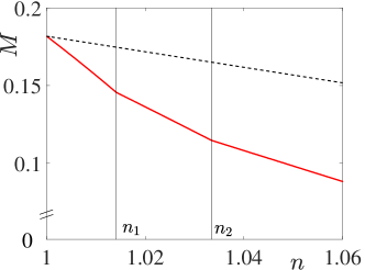
Figure 2: Fig. 2 The dependence of the magnetization $M$ on the electron density (solid line) at $J_{1}=0.5t_{1}$, $J_{2}=0.02t_{1}$ as compared to (dashed line) the result obtained disregarding charge fluctuations. The vertical lines denote the critical concentrations $n_{1}$ and $n_{2}$ for topological transitions in the coexistence phase

The density dependence of the magnetization at the parameters $J_{1}=0.5t_{1}$, $J_{2}=0.02t_{1}$ is shown in Fig. 2 by the solid line. It is seen that hoppings near half filling lead to a stronger decrease in the magnetization with increasing density in comparison with the trivial result $1-n/2$ (dashed line in Fig. 2 is obtained taking into account this result and the contribution from spin fluctuations) in the vicinity of half filling. The vertical lines denote the densities $n_{1}=1.014$ and $n_{2}=1.033$ at which gapless excitations are realized in the coexistence phase. The features of these densities are also manifested in the energy spectrum of fermion states for noncollinear spin ordering. At densities $1<n<n_{1}$ the states are filled near the point $K^{\prime}$ of the Brillouin zone, as it can be seen from Fig. 3. At densities $n_{1}<n<n_{2}$ the filling of states near the $\Gamma$ and $K$ points occurs (see Fig. 4). Due to such density evolution the arising corrections to the magnetization lead to a kink in the dependence $M(n)$ at $n=n_{1}$. Above the density $n_{2}$ the upper band with the minimum at the $K^{\prime}$ point starts to be filled. As a result such processes lead to a a decrease in the slope of the dependence $M(n)$ and the occurrence of the second kink at $n=n_{2}$. The spectrum of the upper band is described by the expression $\varepsilon_{2p}$.

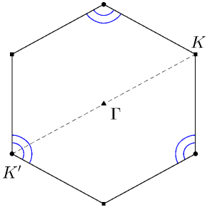
Figure 3: Fig. 3 Fermi contours for densities $1<n<n_{1}$, $n_{11}=1.005$, $n_{12}=1.013$

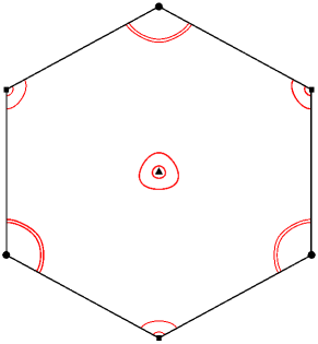
Figure 4: Fig 4 Fermi contours for densities $n_{1}<n<n_{2}$, $n_{21}=1.015$, $n_{22}=1.025$

The fermion spectrum is shown in Figs. 5 and 6 for different values of the density $n=n_{1}$ and $n=n_{2}$, respectively. The spectrum indicates realization of gapless excitations in the coexistence phase. The reported effects argue that the existence of gapless excitations and, accordingly, topological transitions can be revealed by the behavior of the magnetization and related characteristics.

The density dependencies of the amplitude $\Delta_{21}$ describing the superconducting pairings due to the exchange interaction with the first coordination sphere are shown in Fig. 7. The relevant self-consistent equations are given in [26]. In the next section, we show that a topological transition with a change in the topological invariant occurs when the gapless excitations are implemented in the coexistence phase of superconductivity and 120^∘ ordering.

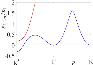
Figure 5: Fig. 5 Fermi spectrum with regard to the noncollinear spin ordering along the $K^{\prime}$-$\Gamma$-$K$ direction of the Brillouin zone for the density $n=n_{1}$. The energy is counted from the chemical potential

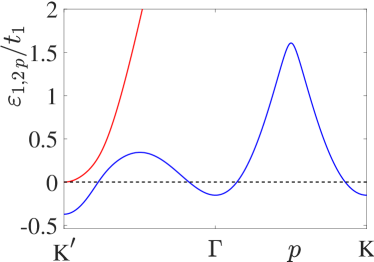
Figure 6: Fig. 6 The Fermi spectrum for the density $n=n_{2}$

5. Topological invariant $\tilde{N}_{3}$ and Majorana modes

To solve the problem of a nontrivial topology of the coexistence phase of superconductivity and noncollinear magnetism at strong electron correlations, we use the method based on the analysis of the integer-valued topological invariant $\tilde{N}_{3}$ [15]:

$$\tilde{N}_{3} = \frac{\varepsilon_{\mu\nu\lambda}}{24\pi^{2}}\times$$

$$\times \int\limits_{-\infty}^{\infty}d\omega\int\limits_{-\pi}^{\pi}dk_{1}dk_{2}\text{Tr}\left(\widehat{G}\partial_{\mu}\widehat{G}^{-1}\widehat{G}\partial_{\nu}\widehat{G}^{-1}\widehat{G}\partial_{\lambda}\widehat{G}^{-1}\right).$$

Here, the repeated indices $\mu$, $\nu$, $\lambda=1,\,2,\,3$ imply summation, $\varepsilon_{\mu\nu\lambda}$ is the Levi-Civita symbol, $\partial_{1}\equiv\partial/\partial k_{1}$, $\partial_{2}\equiv\partial/\partial k_{2}$, $\partial_{3}\equiv\partial/\partial\omega$, and $\widehat{G}(i\omega,k)$ is the matrix Green’s function whose poles determine the spectrum of elementary fermion excitations (details are presented in the supplementary material).

The value $\tilde{N}_{3}=0$ corresponds to the topologically trivial phase. In a topologically nontrivial phase, $\tilde{N}_{3}\neq 0$. Transitions between phases with different $\tilde{N}_{3}$ values are topological transitions.

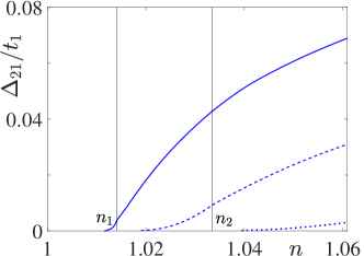
Figure 7: Fig. 7 The dependence of the amplitude $\Delta_{21}$ on density for different values of the parameter of intersite Coulomb repulsion: $V=0$ (solid line), $V=0.3t_{1}$ (dashed line), $V=0.6t_{1}$ (dotted line)

The calculation of the number $\tilde{N_{3}}$ shows that the coexistence phase of superconductivity and 120^∘ spin ordering is topologically nontrivial with $\tilde{N_{3}}\neq 0$. The coexistence phase at $V=0$ occurs in a fairly wide density range (see Fig. 7), but a particular $\tilde{N_{3}}$ value can be different. The sequence of changes in $\tilde{N_{3}}$ upon an increase in the density of fermions is as follows:

$$(\tilde{N_{3}}=-1)~{}~{}{\stackrel{{\scriptstyle n=n_{1}}}{{\longrightarrow}}}~{}~{}(\tilde{N_{3}}=3)~{}~{}{\stackrel{{\scriptstyle n=n_{2}}}{{\longrightarrow}}}~{}~{}(\tilde{N_{3}}=2).$$ (14)

Topological transitions occur at the same parameters at which the bulk spectrum of elementary excitations becomes gapless. It is substantial that these conditions for existence of topological transitions are independent of the magnitude of the superconducting order parameter.

As seen in Fig. 7, different numbers of topological transitions occur in the coexistence phase depending on the parameter $V$. Indeed, at $V=0$, two such transitions occur at the densities $n_{1}$ and $n_{2}$; as $V$ increases to $V=0.3t_{1}$, the transition at $n=n_{1}$ disappears, but the topological transition at the density $n_{2}$ holds; and topological transitions are absent at $V=0.6t_{1}$.

To determine the structure of the Majorana mode, we use a method similar to that used for models disregarding interactions [17]. We consider a system with the triangular lattice containing a finite number ($N_{1}$) of sites along the direction of the translation vector ${\bf a}_{1}$, whereas periodic boundary conditions are imposed along the ${\bf a}_{2}$ direction (cylindrical geometry). According to the solution of the system of equations in the coordinate–momentum representation, the low-energy “quasiparticle” Green’s function can be represented in the form

$$\left(i\omega_{m}-\varepsilon_{jk_{2}}\right)G_{\alpha_{j},\downarrow 2}\left(k_{2};n^{\prime};i\omega_{m}\right)=\left(S^{{\dagger}}\right)_{jn^{\prime}},$$ (15)

where $\varepsilon_{jk_{2}}$ are the branches of the excitation spectrum with $j=1,2,\dots N_{1}$, and $S$ is the transformation matrix diagonalizing the initial matrix of the system of equations.

The relation between the Green’s function found from Eq. (15) and initial Green’s functions in the coordinate–momentum representation makes it possible to determine the operators of elementary excitations for the coexistence phase in the cylindrical geometry in terms of the Hubbard fermion operators:

$$\alpha_{jk_{2}} = \sum_{l=1}^{N_{1}}u_{jl}X_{k_{2},l,\uparrow}+w_{jl}X_{k_{2}-Q_{2},l,\downarrow}$$ (16)

$$+ z_{jl}X^{{\dagger}}_{-k_{2}+Q_{2},l,\uparrow}+v_{jl}X^{{\dagger}}_{-k_{2},l,\downarrow}.$$

According to this definition and symmetry reasons [17], the Majorana mode in the cylindrical geometry occurs at $K_{2}=-K_{2}+Q_{2}+G$, i.e., at $K_{2}=-Q_{2}=-2\pi/3$, when the excitation energy is zero, as seen in Fig. 8.

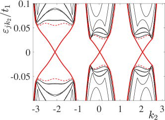
Figure 8: Fig. 8 Spectrum of fermion excitations in the coexistence phase for the cylindrical geometry

The dependences of several branches of the excitation spectrum on the quasimomentum $k_{2}$ at the density $n=1.025$ and $V=0$ are shown in Fig. 8, where the other parameters are the same as those used for Figs. 2 and 7. The dashed line denotes the boundary of the bulk excitation spectrum at periodic boundary conditions along both directions of the triangular lattice. It is seen that the excitation spectrum in this case has an energy gap. Edge states appear inside the spectrum gap (shown by thick solid line) in the cylindrical geometry. Thin solid lines selectively show the branches lying in the region of the bulk spectrum.

For the visualization of the spatial structure of the Majorana mode ($K_{2}=-Q_{2}$), we use the Kitaev approach. To this end, we introduce two Hermitian operators $b^{\prime}=\alpha_{1}+\alpha_{1}^{{\dagger}}$ and $b^{\prime\prime}=i(\alpha_{1}^{{\dagger}}-\alpha_{1})$. Then, using expansion (16), we express these operators in terms of Majorana operators in the atomic representation

$$\gamma_{Al\sigma}=X_{l\sigma}+X^{{\dagger}}_{l\sigma},~{}~{}~{}\gamma_{Bl\sigma}=i\left(X^{{\dagger}}_{l\sigma}-X_{l\sigma}\right).$$ (17)

These transformations give

$$b^{\prime}=\sum_{l=1}^{N_{1}}\left\{Re(u_{1l}+z_{1l})\gamma_{Al\uparrow}+Re(w_{1l}+v_{1l})\gamma_{Al\downarrow}\right\}-$$

$$\sum_{l=1}^{N_{1}}\left\{Im(u_{1l}-z_{1l})\gamma_{Bl\uparrow}+Im(w_{1l}-v_{1l})\gamma_{Bl\downarrow}\right\},$$

$$b^{\prime\prime}=\sum_{l=1}^{N_{1}}\left\{Im(u_{1l}+z_{1l})\gamma_{Al\uparrow}+Im(w_{1l}+v_{1l})\gamma_{Al\downarrow}\right\}+$$

$$\sum_{l=1}^{N_{1}}\left\{Re(u_{1l}-z_{1l})\gamma_{Bl\uparrow}+Re(w_{1l}-v_{1l})\gamma_{Bl\downarrow}\right\}$$

Figure 9 shows the dependence of the coefficients $A_{l}=Re(u_{1l}+z_{1l})$ and $B_{l}=Im(u_{1l}+z_{1l})$ of the decompositions of the operators $b^{\prime}$ and $b^{\prime\prime}$ in Majorana operators in the atomic representation on the site number. It is seen that this dependence is localized near different edges. Other expansion coefficients demonstrate a similar localization and, for this reason, are not shown.

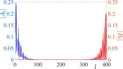
Figure 9: Fig. 9 Coefficients $A_{l}=\text{Re}(u_{1l}+z_{1l})$ and $B_{l}=\text{Im}(u_{1l}+z_{1l})$ versus the site number for the density $n=1.025$ and $N_{1}=400$

After the topological transition to the region with $\tilde{N}_{3}=2$ for densities $n>n_{2}$, a gap for the branch of edge states opens in the excitation spectrum of the finite system at $K_{2}=-Q_{2}$ and the Majorana mode is absent. The Majorana mode also occurs at $K_{2}=-Q_{2}$ in the coexistence phase with $N_{3}=-1$ in the narrow density range $n<n_{1}$. In this region, in contrast to the region with $N_{3}=3$, the branch of edge states is formed only near $K_{2}=-Q_{2}$. However, such topological phase is of low practical interest because the superconducting gap is very narrow even disregarding the intersite Coulomb interaction.

6. Conclusions

The results obtained in this work show that strong electron correlations significantly renormalize the spin structure parameter but do not destroy the coexistence phase of chiral superconductivity and noncollinear magnetic ordering. It has been found that a nontrivial topology also holds in this case, which is important for the formation of Majorana modes in this phase at open boundary conditions. The nontrivial topology has been proven using the topological invariant $\tilde{N_{3}}$ calculated in terms of the Green’s functions determined by means of the Hubbard operators. The atomic representation has made it possible not only to correctly describe the effects of strong electron correlations but also to study the structure of the Majorana mode for the strongly correlated coexistence phase of chiral superconductivity and noncollinear spin ordering by introducing Majorana operators in the atomic representation. The diagrammatic technique for the Hubbard operators has allowed the calculation of contributions from spin and charge fluctuations to the macroscopic characteristic of the magnetic structure. Particular calculations near half filling within the $t-J-V$ model have demonstrated a change in the topological invariant $\tilde{N_{3}}$ at the variation of the electron density. It has been found that the character of a change in $\tilde{N_{3}}$ depends on the intersite Coulomb interaction. An important conclusion has been made from the form of the dependence of $\tilde{N_{3}}$: depending on the model parameters and external conditions, either edges states which are Majorana bound states or edge states which do not belong to the Majorana type can be formed in the coexistence phase. The transition between these two regimes occurs as a quantum topological transition in density.

We are grateful to M.S. Shustin for stimulating discussions. This work was supported by the Russian Foundation for Basic Research (project nos. 19-02- 00348-a and 18-32-00443-mol-a); jointly by the Russian Foundation for Basic Research, the Government of Krasnoyarsk Region, and the Krasnoyarsk Region Science and Technology Support Fund (project no. 18-42-243002 “Manifestation of Spin–Nematic Correlations in Spectral Characteristics of the Electronic Structure and Their Influence on Practical Properties of Cuprate Superconductors”); and by the Presidium of the Russian Academy of Sciences (program no. I.12 “Fundamental Problems of High-Temperature Superconductivity”). A.O.Z. acknowledges the support of the Council of the President of the Russian Federation for State Support of Young Scientists and Leading Scientific Schools (project no. MK-3594.2018.2).

The section 5 and conclusions translated by R. Tyapaev

References

- [1] N. Read, D. Green, Phys. Rev. B 61 10267 (2000).
- [2] A. Yu. Kitaev, Physics-Uspekhi, Suppl. 44, 131 (2001).
- [3] L. Fu, C. L. Kane, Phys. Rev. Lett., 100 096407 (2008).
- [4] M. Snelder, A. A. Golubov, Y. Asano, A. Brinkman, J. Phys.: Condens. Matter 27, 315701 (2015).
- [5] J. D. Sau, R. M. Lutchyn, S. Tewari, S. Das Sarma, Phys. Rev. Lett. 104, 040502 (2010).
- [6] R. M. Lutchyn, J. D. Sau, S. Das Sarma, Phys. Rev. Lett. 105, 077001 (2010).
- [7] M. Sato, S. Fujimoto, Phys. Rev. Lett. 105, 217001 (2010).
- [8] V. V. Val’kov, V. A. Mitskan, and M. S. Shustin, JETP Lett. 106, 798 (2017).
- [9] A. A. Kopasov, I. M. Khaymovich, A. S. Mel’nikov, Beilstein J. Nanotechnol. 9, 1184, (2018).
- [10] H. Zhang, Ch.-X Liu, S. Gazibegovic, Di Xu, J. A. Logan, G. Wang, N. van Loo, J. D. S. Bommer, M. W. A. de Moor, D. Car, R. L. M. Ophet Veld, P. J. van Veldhoven, S. Koelling, M. A. Verheijen, M. Pendharkar, D. J. Pennachio, B. Shojaei, J. S. Lee, Ch. J. Palmstrom, E. P. A. M. Bakkers, S. Das Sarma, L. P. Kouwenhoven, Nature 556, 74 (2018).
- [11] I. Martin, A.F. Morpurgo, Phys. Rev. B 85, 144505 (2012).
- [12] Y.-M. Lu, Z. Wang, Phys. Rev. Lett. 110, 096403 (2013).
- [13] A. P. Schnyder, S. Ryu, A. Furusaki, A. W. W. Ludwig, Phys. Rev. B 78, 195125 (2008).
- [14] P. Ghosh, J.D. Sau, S. Tewari, S. Das Sarma, Phys. Rev. B 82, 184525 (2010).
- [15] G.E. Volovik, The Universe in a Helium Droplet, Oxford Press, New York (2003).
- [16] V. V. Val’kov and A. O. Zlotnikov, JETP Lett. 104, 483 (2016).
- [17] V. V. Val’kov, A. O. Zlotnikov, M.S. Shustin, J. of Magn. Magn. Materials 459, 112 (2018).
- [18] L. Fidkowski, A. Yu. Kitaev, Phys. Rev. B 81, 134509 (2010).
- [19] T. Morimoto, A. Furusaki, Ch. Mudry, Phys. Rev. B 92, 125104 (2015).
- [20] K. Ishikawa, T. Matsuyama, Nucl. Phys. B280, 523 (1987).
- [21] G.E. Volovik, V.M. Yakovenko, J. Phys. Condens. Matter 1, 5263 (1989).
- [22] G. E. Volovik, JETP Letters 90, 398 (2009).
- [23] Z. Wang, S.-C. Zhang, Phys. Rev. B 86, 165116 (2012).
- [24] G. Baskaran, Phys. Rev. Lett. 91, 097003 (2003).
- [25] V. V. Val’kov, T. A. Val’kova, V. A. Mitskan, J. of Magn. Magn. Materials 440, 129 (2017).
- [26] V. V. Val’kov and A. O. Zlotnikov, Phys. Solid State 59, 2120 (2017).
- [27] A. V. Chubukov, S. Sachdev, T. Senthil, J. Phys.: Condens. Matter. 6, 8891 (1994).
- [28] D. M. Dzebisashvili and A. A. Khudaiberdyev, JETP Lett. 108, 189 (2018).
- [29] L. Capriotti, A. E. Trumper, S. Sorella, Phys. Rev. Lett. 82, 3899 (1999).
- [30] S. R. White, A. L. Chernyshev, Phys. Rev. Lett. 99, 127004 (2007).
- [31] A. F. Barabanov, A. V. Mikheyenkov, JETP Lett. 56, 454 (1992).
- [32] K. Pasrija, S. Kumar, Phys. Rev. B 93, 195110 (2016).
- [33] K. Jiang, S. Zhou, Z. Wang, Phys. Rev. B 90, 165135 (2014).
- [34] C. Weber, A. Lauchli, F. Mila, T. Giamarchi, Phys. Rev. B 73, 014519 (2006).
- [35] R. O. Zaitsev, Sov. Phys. JETP 41, 100 (1975).
- [36] R. O. Zaitsev, Sov. Phys. JETP 43, 574 (1976).
- [37] V. V. Val’kov and S. G. Ovchinnikov, Hubbard Operators in the Theory of Strongly Correlated Electrons (Imperial College Press, London, 2004).