Unbiased estimators for random design regression

Abstract

In linear regression we wish to estimate the optimum linear least squares predictor for a distribution over $d$-dimensional input points and real-valued responses, based on a small sample. Under standard random design analysis, where the sample is drawn i.i.d. from the input distribution, the least squares solution for that sample can be viewed as the natural estimator of the optimum. Unfortunately, this estimator almost always incurs an undesirable bias coming from the randomness of the input points, which is a significant bottleneck in model averaging. In this paper we show that it is possible to draw a non-i.i.d. sample of input points such that, regardless of the response model, the least squares solution is an unbiased estimator of the optimum. Moreover, this sample can be produced efficiently by augmenting a previously drawn i.i.d. sample with an additional set of $d$ points, drawn jointly according to a certain determinantal point process constructed from the input distribution rescaled by the squared volume spanned by the points. Motivated by this, we develop a theoretical framework for studying volume-rescaled sampling, and in the process prove a number of new matrix expectation identities. We use them to show that for any input distribution and $\epsilon>0$ there is a random design consisting of $O(d\log d+d/\epsilon)$ points from which an unbiased estimator can be constructed whose expected square loss over the entire distribution is bounded by $1+\epsilon$ times the loss of the optimum.

We provide efficient algorithms for constructing such unbiased estimators in a number of practical settings. In one such setting, we let the input distribution be uniform over a large dataset of $n\gg d$ points. Here, we obtain the first unbiased least squares estimator that can be constructed in time nearly-linear in the data size, resulting in strong guarantees for model averaging. We achieve these computational gains by introducing a new algorithmic technique, called distortion-free intermediate sampling, which is the first method to enable sampling from determinantal point processes in time polynomial in the sample size.

Keywords: volume sampling, determinantal point process, linear regression, unbiased estimators, random design.

1 Introduction

We consider linear regression where the examples $(\mathbf{x}^{\scriptscriptstyle{\top}},y)\in\mathbb{R}^{d}\times\mathbb{R}$ are generated by an unknown distribution $\mathrm{D}$ over $\mathbb{R}^{d}\times\mathbb{R}$, with $\mathrm{D}_{\!\cal X}$ denoting the marginal distribution of a row vector $\mathbf{x}^{\scriptscriptstyle{\top}}$ and $\mathrm{D}_{\!\cal Y|\mathbf{x}}$ denoting the conditional distribution of $y$ given $\mathbf{x}$. In statistics, it is common to assume that the response $y$ is a linear function of $\mathbf{x}$ plus zero-mean Gaussian noise; the goal is then to estimate this linear function. We decidedly make no such assumption. Instead, we allow the distribution to be arbitrary except for the nominal requirement that the second moments of the point $\mathbf{x}$ and response $y$ are bounded, i.e., $\mathbb{E}[\|\mathbf{x}\|^{2}]<\infty$ and $\mathbb{E}[y^{2}]<\infty$. The target of the estimation is the linear least squares predictor of $y$ from $\mathbf{x}$ with respect to $\mathrm{D}$:

$$\mathbf{w}^{*}_{\mathrm{D}}\stackrel{{\scriptstyle\textit{\tiny{def}}}}{{=}}\operatorname*{\mathop{\mathrm{argmin}}}_{\mathbf{w}\in\mathbb{R}^{d}}L_{\mathrm{D}}(\mathbf{w}),\quad\text{where}\;\;L_{\mathrm{D}}(\mathbf{w})\stackrel{{\scriptstyle\textit{\tiny{def}}}}{{=}}\mathbb{E}\big{[}(\mathbf{x}^{\scriptscriptstyle{\top}}\mathbf{w}-\mathbf{y})^{2}\big{]}.$$

Here, we assume $\mathbb{E}[\mathbf{x}\mathbf{x}^{\scriptscriptstyle{\top}}]$ is invertible so we have the concise formula $\mathbf{w}^{*}_{\mathrm{D}}=(\mathbb{E}[\mathbf{x}\mathbf{x}^{\scriptscriptstyle{\top}}])^{-1}\mathbb{E}[\mathbf{x}y]$. Our goal is to construct a “good” estimator of this target $\mathbf{w}^{*}_{\mathrm{D}}$ from a small sample. For the rest of the paper we use $\mathbf{w}^{*}$ as a shorthand.

In our setup, the estimator $\widehat{\mathbf{w}}$ of $\mathbf{w}^{*}$ is based on solving a least squares problem on a sample of $k$ examples $(\mathbf{x}_{1}^{\scriptscriptstyle{\top}},y_{1}),\dotsc,(\mathbf{x}_{k}^{\scriptscriptstyle{\top}},y_{k})$. We assume that given $\mathbf{x}_{1},\dotsc,\mathbf{x}_{k}$, the responses $y_{1},\dotsc,y_{k}$ are conditionally independent, and the conditional distribution of $y_{i}$ only depends on $\mathbf{x}_{i}$, i.e., $y_{i}\sim\mathrm{D}_{\!\mathcal{Y}|\mathbf{x}_{i}}$ for $i=1,\dotsc,k$. However, for the applications we have in mind, the marginal distribution of $\mathbf{x}_{1},\dotsc,\mathbf{x}_{k}$ is allowed to be flexibly designed based on $\mathrm{D}_{\!\cal X}$. The most standard choice is i.i.d. sampling from the distribution $\mathrm{D}_{\!\cal X}$ of $\mathbf{x}$, i.e., $(\mathbf{x}_{1}^{\scriptscriptstyle{\top}},\dotsc,\mathbf{x}_{k}^{\scriptscriptstyle{\top}})\sim\mathrm{D}_{\!\cal X}^{k}$. We shall seek other choices that can be implemented given the ability to sample from $\mathrm{D}_{\!\cal X}$ but that lead to better statistical properties for $\widehat{\mathbf{w}}$.

In particular, the properties we want of the estimator $\widehat{\mathbf{w}}$ are the following.

1. Unbiasedness:  $\mathbb{E}[\widehat{\mathbf{w}}]=\mathbf{w}^{*}$.

2. Near-optimal expected loss:  $\mathbb{E}\big{[}L_{\mathrm{D}}(\widehat{\mathbf{w}})\big{]}\leq(1+\epsilon)L_{\mathrm{D}}(\mathbf{w}^{*})$ for some (small) $\epsilon>0$.

Together, these properties have many useful implications, such as a bound on the out-of-sample prediction variance, i.e., $\mathrm{Var}[\mathbf{x}^{\scriptscriptstyle{\top}}\widehat{\mathbf{w}}]\leq\epsilon$ for $\mathbf{x}^{\scriptscriptstyle{\top}}\sim\mathrm{D}_{\!\cal X}$, and improved guarantees for averaging, e.g., $\mathbb{E}\big{[}L_{\mathrm{D}}(\frac{\widehat{\mathbf{w}}_{1}+\widehat{\mathbf{w}}_{2}}{2})\big{]}\leq(1+\frac{\epsilon}{2})L_{\mathrm{D}}(\mathbf{w}^{*})$, where $\widehat{\mathbf{w}}_{1}$ and $\widehat{\mathbf{w}}_{2}$ are independent copies of $\widehat{\mathbf{w}}$. The central question is how to sample $\mathbf{x}_{1},\dotsc,\mathbf{x}_{k}$ to achieve these properties with sample size $k=k(\epsilon)$ as small as possible. Note that while in general it is very natural to seek an unbiased estimator, in the context of random design regression it is highly unusual. This is because, as we discuss shortly, standard approaches fail in this regard. In fact, until recently, unbiased estimators have been considered out of reach for this problem.

An important and motivating case of our general setup occurs when $\mathrm{D}_{\!\cal X}$ is the uniform distribution over a fixed set of $n$ points and $\mathrm{D}_{\!\cal Y|\mathbf{x}}$ is deterministic. That is, there is an $n\times d$ fixed design matrix $\mathbf{X}$ and a response vector $\mathbf{y}\in\mathbb{R}^{n}$ such that the distribution is uniform over the $n$ rows. Here, the loss of $\mathbf{w}$ can be written as $L_{\mathrm{D}}(\mathbf{w})=\tfrac{1}{n}\|\mathbf{X}\mathbf{w}-\mathbf{y}\|^{2}$. This traditionally fixed design setting turns into a random design when we are required to sample $k\ll n$ rows of $\mathbf{X}$, observe only the entries of $\mathbf{y}$ corresponding to those rows, and then construct an estimate $\widehat{\mathbf{w}}$ of the least squares solution for all of $(\mathbf{X},\mathbf{y})$. Such constraints are imposed either in the context of experimental design and active learning, where $k$ represents the budget of responses that we are allowed to observe (e.g., because the responses are expensive), or to reduce the computational cost of solving the full least squares problem. Here, an important motivation for unbiasedness is parallel and distributed model averaging, where we wish to aggragate many independent copies of an estimator. See Section 1.2 for further discussion of model averaging and experimental design.

Throughout the introduction we give some intuition about our results by discussing the one dimensional case. For example, consider the following $2\times 1$ fixed design problem:

$$\mathbf{X}=\begin{bmatrix}\text{$x_{1}\!\!\mathrel{\mathop{\mathchar 58\relax}}$}\ 1\ \\ \text{$x_{2}\!\!\mathrel{\mathop{\mathchar 58\relax}}$}\ 2\ \end{bmatrix},\quad\mathbf{y}=\begin{bmatrix}\text{$y_{1}\!\!\mathrel{\mathop{\mathchar 58\relax}}$}\ 1\ \\ \text{$y_{2}\!\!\mathrel{\mathop{\mathchar 58\relax}}$}\ 1\ \end{bmatrix},\quad\text{with target:}\quad\mathbf{w}^{*}=\frac{\sum_{i}x_{i}y_{i}}{\sum_{i}x_{i}^{2}}=\frac{3}{5}.$$ (1.1)

Suppose that we wish to estimate the target after observing only a single response (i.e., $k=1$). If we draw the response uniformly at random (i.e., from the distribution $\mathrm{D}$), then the least squares estimator for this sample will be a biased estimate of the target: $\mathbb{E}[\widehat{\mathbf{w}}]=\frac{1}{2}\frac{y_{1}}{x_{1}}+\frac{1}{2}\frac{y_{2}}{x_{2}}=\frac{3}{4}\neq\frac{3}{5}.$

The bias in least squares estimators is present even when each input component is drawn independently from a standard Gaussian. As an example, we let $d=5$ and set:

$$\mathbf{x}^{\scriptscriptstyle{\top}}\!=(x_{1},\dots,x_{d})\overset{\text{i.i.d.}}{\sim}\mathcal{N}(0,1),\quad\ y=\xi(\mathbf{x})\!+\!\epsilon,\quad\text{where }\ \xi(\mathbf{x})=\sum_{i=1}^{d}x_{i}+\frac{x_{i}^{3}}{3},\quad\epsilon\sim\mathcal{N}(0,1).$$

The response $y$ is a non-linear function $\xi(\mathbf{x})$ plus independent white noise $\epsilon$. Note that it is crucial that the response contains some non-linearity, and it is something that one would expect in real datasets. The response is cubic and was chosen so that it is easy to solve algebraically for the optimum solution $\mathbf{w}^{*}=\operatorname*{\mathop{\mathrm{argmin}}}_{\mathbf{w}}L_{\mathrm{D}}(\mathbf{w})$ (see Appendix A).

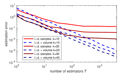
Figure 1.1: Averaging least squares estimators for Gaussian inputs with $d=5$.

For this Gaussian setup we evaluate the bias of the least squares estimator produced for this problem by i.i.d. sampling of $k$ points. We do this by performing model averaging, i.e., producing many such estimators $\widehat{\mathbf{w}}_{1},\dots,\widehat{\mathbf{w}}_{T}$ independently, and looking at the estimation error of the average of those estimators $\widetilde{\mathbf{w}}\mathrel{\mathop{\mathchar 58\relax}}=\frac{1}{T}\sum_{t=1}^{T}\widehat{\mathbf{w}}_{t}$:

$$\text{estimation error:}\quad\|\widetilde{\mathbf{w}}-\mathbf{w}^{*}\|^{2}.$$

Figure 1.1 (red curves) shows the experiment for several values of $k$ and a range of values of $T$ (each presented data point is an average over 50 runs). The i.i.d. sampled estimator is biased for any sample size (although the bias decreases with $k$), and therefore the averaged estimator clearly does not converge to the optimum. We next discuss how to construct an unbiased estimator (dashed blue curves), for which the estimation error of the averaged estimator exhibits $\frac{1}{T}$ convergence to zero (regardless of $k$). This type of convergence appears as a straight line on the log-log plot on Figure 1.1.

Recently, Dereziński and Warmuth (2018) developed the first method for constructing unbiased estimators in the case where $\mathrm{D}$ is uniform over a fixed design $(\mathbf{X},\mathbf{y})$. This method, which we will refer to as discrete volume sampling, jointly draws a subset $S\subseteq[n]$ of $k$ rows of the design matrix $\mathbf{X}$ with probability proportional to $\det(\mathbf{X}_{S}^{\scriptscriptstyle{\top}}\mathbf{X}_{S})$, where $\mathbf{X}_{S}$ denotes the submatrix of $\mathbf{X}$ with rows indexed by $S$. For this distribution, the linear least squares estimator $\widehat{\mathbf{w}}=\mathbf{X}_{S}^{\dagger}\mathbf{y}_{S}$ is unbiased, i.e., $\mathbb{E}[\widehat{\mathbf{w}}]=\mathbf{w}^{*}=\mathbf{X}^{\dagger}\mathbf{y}$, where $\mathbf{X}^{\dagger}$ denotes the Moore-Penrose pseudoinverse. Indeed, if we volume sample the set $S$ of size 1 in the example problem (1.1), then $\mathbb{E}[\widehat{\mathbf{w}}]=\frac{x_{1}^{2}}{\sum_{i}x_{i}^{2}}\,\frac{x_{1}y_{1}}{x_{1}^{2}}+\frac{x_{2}^{2}}{\sum_{i}x_{i}^{2}}\,\frac{x_{2}y_{2}}{x_{2}^{2}}=\frac{\sum_{i}x_{i}y_{i}}{\sum_{i}x_{i}^{2}}=\mathbf{w}^{*}$.

1.1 Our contributions

Contribution 1: Unbiased estimator for random design regression

Our first contribution in this paper is proposing a new unbiased estimator for arbitrary distributions $\mathrm{D}$ (i.e., not just uniform over a fixed design matrix). Let the sample $\mathbf{x}_{1},\ldots,\mathbf{x}_{k}\in\mathbb{R}^{d}$ be drawn jointly with probability proportional to $\det(\sum_{i=1}^{k}\mathbf{x}_{i}\mathbf{x}_{i}^{\scriptscriptstyle{\top}})\,\mathrm{D}_{\!\cal X}^{k}(\mathbf{x}_{1},\ldots,\mathbf{x}_{k})$, i.e., we reweigh the $k$-fold i.i.d. distribution $\mathrm{D}_{\!\cal X}^{k}$ by the determinant of the sample covariance. We refer to this as volume-rescaled sampling from $\mathrm{D}_{\!\cal X}^{k}$ and denote it as ${\mathrm{VS}_{\!\mathrm{D}_{\!\cal X}}^{k}}$. In this general context, we are able to prove that for arbitrary distributions $\mathrm{D}_{\!\cal X}$ and $\mathrm{D}_{\!\cal Y|\mathbf{x}}$, volume-rescaled sampling produces unbiased linear least squares estimators (Theorem 2.10). This result does not follow from the fixed design analysis, and in obtaining it we derive novel extensions of fundamental expectation identities for the determinant of a random matrix. In the process, we develop a new tool kit for computing expectations under volume-rescaled sampling, which includes new expectation formulas for sampled pseudoinverses, inverses and adjugates.

Contribution 2: Correcting the bias of i.i.d. sampling

The fact that volume-rescaled sampling of size $k\geq d$ always produces unbiased estimators of the target $\mathbf{w}^{*}$ stands in contrast to i.i.d. sampling from $\mathrm{D}_{\!\cal X}$ which generally fails in this regard. Yet surprisingly, we show that a volume-rescaled sample of any size $k\geq d$ is essentially composed of an i.i.d. sample of size $k-d$ from $\mathrm{D}_{\!\cal X}$ plus a volume-rescaled sample of size $d$ (Theorem 2.4). This means that the linear least squares estimator of such composed sample is also unbiased. Thus, as an immediate corollary of Theorems 2.4 and 2.10 we reach the following remarkable conclusion:

Even though i.i.d. sampling typically results in a biased least squares estimator, adding a volume-rescaled sample of size $d$ to the i.i.d. sample eliminates that bias altogether:

   i.i.d. sample $\displaystyle(\mathbf{x}_{1}^{\scriptscriptstyle{\top}},y_{1}),\ldots,(\mathbf{x}_{k}^{\scriptscriptstyle{\top}},y_{k})\sim D^{k}$ sol. for i.i.d. sample $\displaystyle\widehat{\mathbf{w}}=\operatorname*{\mathop{\mathrm{argmin}}}_{\mathbf{w}}\sum_{i}(\mathbf{x}_{i}^{\scriptscriptstyle{\top}}\mathbf{w}-y_{i})^{2}$ volume-rescaled sample $\displaystyle\overset{\text{$d$ points}}{\bar{\mathbf{x}}_{1}^{\scriptscriptstyle{\top}},\dots,\bar{\mathbf{x}}_{d}^{\scriptscriptstyle{\top}}}\ \sim\ \det\!\text{$\begin{pmatrix}-\bar{\mathbf{x}}_{1}^{\scriptscriptstyle{\top}}-\\ \dots\\ -\bar{\mathbf{x}}_{d}^{\scriptscriptstyle{\top}}-\end{pmatrix}^{\!\!\!2}$}\!\cdot\mathrm{D}_{\!\cal X}^{d}\ \ \,\text{\scriptsize($d$ - input dimension)}$ query responses $\displaystyle\bar{y}_{i}\ \sim\ \mathrm{D}_{{\cal Y}|\bar{\mathbf{x}}_{i}},\quad\forall_{i=1..d}$ sol. for i.i.d + volume $\displaystyle\widetilde{\mathbf{w}}=\operatorname*{\mathop{\mathrm{argmin}}}_{\mathbf{w}}\Big{\{}\sum_{i}(\mathbf{x}_{i}^{\scriptscriptstyle{\top}}\mathbf{w}-y_{i})^{2}+\sum_{i}(\bar{\mathbf{x}}_{i}^{\scriptscriptstyle{\top}}\mathbf{w}-\bar{y}_{i})^{2}\Big{\}}$   Our result: $\mathbb{E}[\widetilde{\mathbf{w}}]=\mathbf{w}^{*}$ even though typically $\mathbb{E}[\widehat{\mathbf{w}}]\neq\mathbf{w}^{*}$

Indeed, in the simple Gaussian experiment used for Figure 1.1, the estimators produced from i.i.d. samples augmented with a volume-rescaled sample of size $d$ (dashed blue curves) become unbiased (straight lines). To get some intuition, let us show how the bias disappears in the one-dimensional fixed design case where $\mathrm{D}_{\!\cal X}$ is a uniform sample from $\{(x_{1},y_{1}),\dots,(x_{n},y_{n})\}$. In this case, reweighing the probability of just the first sampled point by its square already results in an unbiased estimator. Let $\widehat{\mathbf{w}}$ be the least squares estimator computed from $(x_{i_{1}},y_{i_{1}}),\dots,(x_{i_{k}},y_{i_{k}})$ with all indices sampled uniformly from $[n]$. Now, suppose that we replace $i_{1}$ with $i_{1}^{\prime}$ sampled proportionally to $x_{i_{1}^{\prime}}^{2}$, and denote the modified estimator as $\widetilde{\mathbf{w}}$. Due to symmetry, it makes no difference which index we choose to replace, so

$$\mathbb{E}\big{[}\widetilde{\mathbf{w}}\big{]}=\mathbb{E}\Big{[}\tfrac{x^{2}_{i_{1}}}{\sum_{j}x_{j}^{2}}\,\widehat{\mathbf{w}}\Big{]}=\frac{1}{k}\sum_{t=1}^{k}\mathbb{E}\Big{[}\tfrac{x^{2}_{i_{t}}}{\sum_{j}x_{j}^{2}}\,\widehat{\mathbf{w}}\Big{]}=\frac{\mathbb{E}[\frac{1}{k}(\sum_{t}x_{i_{t}}^{2})\,\widehat{\mathbf{w}}]}{\sum_{j}x_{j}^{2}}.$$

By definition of the least squares estimator, $\mathbb{E}[\frac{1}{k}(\sum_{t}x_{i_{t}}^{2})\,\widehat{\mathbf{w}}]=\mathbb{E}[\frac{1}{k}\sum_{t}x_{i_{t}}y_{i_{y}}]=\sum_{j}x_{j}y_{j}$, from which it follows that $\mathbb{E}[\widetilde{\mathbf{w}}]=\mathbf{w}^{*}.$ This simple argument at once shows the unbiasedness of $\widetilde{\mathbf{w}}$ and the composition property discussed in the previous paragraph. In higher dimensions, the analysis gets considerably more involved, but it follows a similar outline.

Contribution 3: Near-optimal expected loss bound

Perhaps surprisingly, volume-rescaled sampling may not lead to estimators with near-optimal loss guarantees: We show that for any $k\geq d$ there are distributions $D$ for which volume-rescaled sampling of size $k$ results in the linear least squares estimator having loss at least twice as large as the optimum loss (with probability at least 0.25). However, we remedy this bad behavior by composing a volume-rescaled sample of size $d$ with an i.i.d. leverage score sample of size $k-d$. This composition achieves the following feat: It does not affect the unbiasedness of the estimator and, and it leads to good approximation properties. Specifically, in Theorem 3.1 we show that $k=O(d\log d+d/\epsilon)$ points are sufficient to construct an estimator $\widehat{\mathbf{w}}$ such that:

$$\mathbb{E}[\widehat{\mathbf{w}}]=\mathbf{w}^{*}\quad\text{and}\quad\mathbb{E}\big{[}L_{\mathrm{D}}(\widehat{\mathbf{w}})\big{]}\leq(1+\epsilon)L_{\mathrm{D}}(\mathbf{w}^{*}).$$

Note that an analogous loss bound is achievable for vanilla i.i.d. leverage score sampling, but (1) the estimators produced from leverage score sampling are biased, and (2) the expected loss bound holds only if we condition on a certain high-probability event (both of those are significant issues, e.g., in the context of model averaging). To show the expected loss bound that holds without conditioning and for an unbiased estimator, we break the analysis into two cases, depending on whether the high-probability event occurs. When it does not, then our analysis crucially relies on the expectation formulas we develop for volume-rescaled sampling. Note that the only expected loss bound previously developed for a volume-based sampling distribution was limited to fixed design, and required $d^{2}/\epsilon$ points to obtain an approximation factor of $1+\epsilon$ (Dereziński and Warmuth, 2018). To our knowledge, that analysis does not easily extend to $k>d$, which is why our techniques are radically different.

Contribution 4: Accelerated sampling algorithms

Our work also leads to sampling algorithms which significantly improve on the state-of-the-art time complexity of volume-rescaled sampling, both in the fixed and random design settings, with further algorithmic implications for the broader class of determinantal point processes (see Section 1.2.3). We achieve this by introducing a new technique called distortion-free intermediate sampling: We first sample a larger pool of points based on approximate i.i.d. leverage scores and then down-sample from that pool to construct the volume-rescaled sample. We use rejection sampling for the down-sampling step to ensure exactness of the resulting overall sampling distribution. Surprisingly, this does not adversely affect the complexity because of the provably high acceptance rate during rejection sampling (see Theorem 5.6).

When distribution $\mathrm{D}$ is defined by a fixed design $(\mathbf{X},\mathbf{y})$ with $n\gg d$ data points, then, in Theorem 5.9, we improve upon the time complexity of discrete volume sampling from $O(nd^{2})$ to $O(nd\log n+d^{4}\log d)$. This cost is nearly-linear in the size of the dataset and, for the first time, better than solving the full least squares problem directly, which takes $O(nd^{2})$ time. Importantly, most of the cost in the new algorithm comes from preprocessing, and the actual sampling takes only $O(d^{4})$ time, i.e., independent of the data size, which is useful when we wish to produce multiple independent samples. Combining this with the new loss bound, we get the following improvements for obtaining an unbiased subsampled estimator with loss within $1+\epsilon$ of the optimum: The sample size $k$ is reduced from $O(d^{2}/\epsilon)$ to $O(d\log d+d/\epsilon)$ and the time complexity from $O(nd^{3}/\epsilon)$ to $O(nd\log n+d^{4}\log d+d^{3}/\epsilon)$.

Remarkably, we show that exact volume-rescaled sampling is possible even when distribution $\mathrm{D}_{\!\cal X}$ is unknown (and possibly continuous) and we only have oracle access to it. In this setting, the size of the intermediate sample that is necessary to achieve this grows linearly with a certain condition number of the distribution (this is likely unavoidable in general). Finally, in the special case where $\mathrm{D}_{\!\cal X}$ is a multivariate Gaussian distribution with unknown covariance, we use a different approach to show that only $d+2$ additional samples from $\mathrm{D}_{\!\cal X}$ are needed to modify a sample from $\mathrm{D}_{\!\cal X}^{k}$ so that it becomes a volume-rescaled sample of size $k$.

1.2 Applications of our results

While studying unbiased estimators for least squares regression is an old and classical problem, our new results have significant implications for modern data science, both from a computational and statistical perspective. We outline these implications below, along with some of the recent related work.

1.2.1 Model averaging

Model averaging is a standard technique for boosting the accuracy of a subsampled estimator by constructing multiple independent copies and then averaging them. This is particularly effective in parallel and distributed environments, where the computational cost of constructing multiple estimators is the same as the cost of computing one estimator. While model averaging has been proposed as a strategy for least squares regression (e.g., see Wang et al., 2017a), the bias which arises for commonly used estimators (e.g., based on i.i.d. sampling) constitutes a significant bottleneck for this approach.

Our framework for constructing unbiased estimators with expected loss bounds is uniquely suited for addressing the problem of estimation bias in model averaging. To see this, consider a least squares estimator $\widehat{\mathbf{w}}$ that satisfies both the unbiasedness property, $\mathbb{E}[\widehat{\mathbf{w}}]=\mathbf{w}^{*}$, and near-optimal expected loss, $\mathbb{E}[L_{\mathrm{D}}(\widehat{\mathbf{w}})]\leq(1+\epsilon)L_{\mathrm{D}}(\mathbf{w}^{*})$. It immediately follows that if we construct $m$ independent copies $\widehat{\mathbf{w}}_{1},...,\widehat{\mathbf{w}}_{m}$ of $\widehat{\mathbf{w}}$, then the averaged estimator satisfies:

$$\mathbb{E}\big{[}L_{\mathrm{D}}(\widetilde{\mathbf{w}})\big{]}\leq\Big{(}1+\frac{\epsilon}{m}\Big{)}\,L_{\mathrm{D}}(\mathbf{w}^{*}),\quad\text{where}\quad\widetilde{\mathbf{w}}=\frac{1}{m}\sum_{i=1}^{m}\widehat{\mathbf{w}}_{i}.$$

Consider for instance the setting where distribution $\mathrm{D}$ is defined by a fixed design $(\mathbf{X},\mathbf{y})$ with $n$ data points. Here, we can use parallel averaging to boost the accuracy of a subsampled least squares estimator from $\epsilon$ to $\epsilon/m$ at virtually no additional computational cost. However, for this to be practical, (1) the estimator must be unbiased, and (2) the computational cost of constructing the estimator must be less than $O(nd^{2})$, the cost of solving least squares exactly. We develop the first such estimator, by not only providing an improved expected loss bound for an unbiased estimator, but also reducing the computational cost to $O(nd\log n+d^{4}\log d)$, which is much less than $O(nd^{2})$ when $n$ is sufficiently larger than $d$. Finally, we point out that our volume-based sampling algorithms for model averaging have recently proven relevant in the context of model averaging for distributed second-order optimization and distributed ridge regression, among others (Dereziński et al., 2020a).

1.2.2 Experimental design

A natural application for volume-rescaled sampling algorithms comes in the context of experimental design (a.k.a. optimal design of experiments; see Fedorov, 1972; Pukelsheim, 2006). Here, the goal is to select a small set of data points for which the least squares estimator minimizes a given optimality criterion, typically related to some notion of variance. Classical experimental design imposes statistical assumptions on the response model, making the least squares estimator trivially unbiased regardless of how we select the set of points. Volume-rescaled sampling provides a way of preserving the unbiasedness property while relaxing the assumptions on the responses. In particular, this leads to a fundamental connection between the expected loss and the prediction variance, a standard optimality criterion (V-optimality) in experimental design. Namely, for an estimator $\widehat{\mathbf{w}}$ such that $\mathbb{E}[\widehat{\mathbf{w}}]=\mathbf{w}^{*}$, letting $\mathbf{x}^{\scriptscriptstyle{\top}}\sim\mathrm{D}_{\!\cal X}$, we have:

$$\underbrace{\mathbb{E}\big{[}L_{\mathrm{D}}(\widehat{\mathbf{w}})\big{]}-L_{\mathrm{D}}(\mathbf{w}^{*})}_{\text{Excess loss}}\hskip 5.69054pt=\underbrace{\mathrm{Var}[\mathbf{x}^{\scriptscriptstyle{\top}}\widehat{\mathbf{w}}]}_{\text{Prediction variance}}.$$

In a recent follow-up work, Dereziński et al. (2019) used these ideas to develop a general framework for experimental design, which bridges the gap between the statistical perspective (linear response model) and the setting studied here (arbitrary responses), relying on our volume-rescaled sampling tool kit (in particular, Theorem 2.4). Furthermore, our strategy of combining volume-based sampling methods with i.i.d. importance sampling (e.g., leverage scores) has proven instrumental in developing randomized rounding methods for efficiently solving a range of experimental design problems (including A/C/D/V-optimal design, and Bayesian experimental design), drastically reducing their computational cost and improving the approximation quality, both for discrete (Nikolov et al., 2019; Dereziński et al., 2020b) and continuous domains (Poinas and Bardenet, 2020).

1.2.3 Determinantal point processes

Volume-rescaled sampling of size $d$ (i.e., ${\mathrm{VS}_{\!\mathrm{D}_{\!\cal X}}^{d}}$, see Definition 2.1) belongs to a family of distributions called Determinantal Point Processes (DPPs), which has been studied extensively in many computational areas as a tractable model of diverse sampling, including in randomized numerical linear algebra (Dereziński and Mahoney, 2021), machine learning (Kulesza and Taskar, 2012) and statistics (Bardenet et al., 2017); here we cite selected surveys that provide a thorough literature review. Our results lead to direct improvements in the computational cost of sampling for an important class of so-called Projection DPPs. We outline this here for the case where the support of the distribution is a finite set.

Determinantal point processes are most commonly defined as a distribution over subsets $S\subseteq\{1,...,n\}$, parameterized by a positive semidefinite $n\times n$ kernel matrix $\mathbf{K}$ with all eigenvalues in $[0,1]$, so that a sample $S\sim\mathrm{DPP}(\mathbf{K})$ satisfies:

$$\mathrm{Pr}(T\subseteq S)=\det(\mathbf{K}_{T,T}),\quad\text{for all}\quad T\subseteq\{1,...,n\}.$$

Here, $\mathbf{K}_{T,T}$ denotes the $|T|\times|T|$ submatrix of $\mathbf{K}$ indexed by $T$. When $\mathbf{K}$ is a projection matrix, i.e., all of its eigenvalues are in $\{0,1\}$, then this is called a Projection DPP and the size of the sampled set $S$ is equal to the rank of $\mathbf{K}$. An alternate parameterization of a Projection DPP that appears in the literature relies on an $n\times d$ matrix $\mathbf{X}$ such that the kernel $\mathbf{K}=\mathbf{X}\mathbf{X}^{\dagger}$ is the rank $d$ projection onto the column span of $\mathbf{X}$. By letting $\mathrm{D}_{\!\cal X}$ be uniform over the rows of $\mathbf{X}$, we obtain that ${\mathrm{VS}_{\!\mathrm{D}_{\!\cal X}}^{d}}$ is the distribution of $\mathbf{X}_{S}$ for $S\sim\mathrm{DPP}(\mathbf{K})$, up to a permutation of the rows (here, $\mathbf{X}_{S}$ indicates the rows of $\mathbf{X}$ indexed by $S$).

Prior to our work, the cost of generating each sample from a given Projection DPP was $O(nd^{2})$, both for the $\mathbf{X}$ and the $\mathbf{K}$ parameterizations, by using the algorithm of Hough et al. (2006). Our technique of distortion-free intermediate sampling drastically reduces these costs when $n\gg d$. If we are using the $\mathbf{X}$ parameterization, then after an initial preprocessing cost of $O(nd\log n+d^{4}\log d)$, we can sample from a Projection DPP in time $O(d^{4})$. When given an $n\times n$ projection matrix $\mathbf{K}$ of rank $d$, we can sample from $\mathrm{DPP}(\mathbf{K})$ in time $O(d^{6})$. Here, the preprocessing step involves simply reading the diagonal of $\mathbf{K}$ in $O(n)$ time. In both cases, these are the first ${\mathrm{poly}}(d)$ time sampling algorithms for Projection DPPs. Follow-up works (Dereziński, 2019; Dereziński et al., 2019; Calandriello et al., 2020) have extended distortion-free intermediate sampling to the class of L-ensemble DPPs, and more recently even beyond DPPs, to larger distribution families such as strongly Rayleigh measures, which have many applications in machine learning and theoretical computer science (Anari and Dereziński, 2020; Anari et al., 2022).

1.3 Related work

A discrete variant of volume-rescaled sampling of size $k=d$ was introduced to computer science literature by Deshpande et al. (2006) for sampling from a finite set of $n$ vectors, with algorithms given later by Deshpande and Rademacher (2010); Guruswami and Sinop (2012). A first extension to samples of size $k>d$ is due to Avron and Boutsidis (2013), with algorithms by Li et al. (2017); Dereziński and Warmuth (2018); Dereziński et al. (2018), and additional applications in experimental design explored by Wang et al. (2017b); Nikolov et al. (2019); Mariet and Sra (2017). Prior to this work, the best known time complexity for this sampling method, called here discrete volume sampling, was $O(nd^{2})$, as shown by Dereziński and Warmuth (2018). Here, we give an $O(nd\log n+d^{4}\log d)$ time algorithm.

As discussed in Section 1.2.3, volume-rescaled sampling of size $d$ is also known in the literature as a type of determinantal point process, called Projection DPP (to learn more, see Dereziński and Mahoney, 2021). Projection DPPs arise in many computational tasks outside of linear regression, such as dimensionality reduction (Belhadji et al., 2020), numerical integration (Bardenet and Hardy, 2020) and graph algorithms (Guenoche, 1983), therefore, efficient sampling algorithms for these distributions are of significant interest (Gautier et al., 2017). More broadly, determinantal point processes have found machine learning applications in recommendation systems (e.g., Gartrell et al., 2016), data summarization (e.g., Gong et al., 2014), stochastic optimization (e.g., Zhang et al., 2017; Mutný et al., 2020), and many others (see Kulesza and Taskar, 2012). The algorithmic technique of distortion-free intermediate sampling, introduced in this work, has already been applied beyond Projection DPPs (Dereziński et al., 2019; Calandriello et al., 2020), which makes it relevant to all of these applications.

The unbiasedness of least squares estimators under volume-based distributions was first explored in the context of sampling from finite datasets by Dereziński and Warmuth (2018), drawing on observations of Ben-Tal and Teboulle (1990). Focusing on small sample sizes, Dereziński and Warmuth (2018) proved multiplicative bounds for the expected loss under sample size $k=d$ with discrete volume sampling. Because the produced estimators are unbiased, averaging $d/\epsilon$ such estimators results in an unbiased estimator based on a sample of size $k=d^{2}/\epsilon$ with expected loss at most $1+\epsilon$ times the optimum at a total sampling cost of $O(nd^{2}\cdot d/\epsilon)$. In contrast, our new techniques achieve an unbiased estimator with sample size $O(d\log d+d/\epsilon)$ and time complexity $O(nd\log n+d^{4}\log d+d^{3}/\epsilon)$. Dereziński and Warmuth (2018) also showed additional variance bounds for discrete volume sampling under the assumption that the responses are linear functions of the input points plus white noise. We extend them here to arbitrary volume-rescaled sampling w.r.t. a distribution.

Other techniques applicable to our linear regression problem include leverage score sampling (Drineas et al., 2006) and algorithms based on spectral sparsification (e.g., Chen and Price, 2019; Kacham and Woodruff, 2020). Leverage score sampling is an i.i.d. sampling procedure which achieves loss bounds nearly matching the ones we obtain here for volume-rescaled sampling, however it produces biased estimators and experimental results (see Section 6) show that it has weaker performance for small sample sizes. A different and more elaborate sampling technique based on spectral sparsification (Batson et al., 2012; Lee and Sun, 2015) was recently shown to be effective for linear regression (Chen and Price, 2019): They show that $O(d/\epsilon)$ samples suffice to produce an estimator with expected loss $(1+\epsilon)L_{\mathrm{D}}(\mathbf{w}^{*})$. However this method also does not produce unbiased estimators, which is a primary concern of this paper and desirable in many settings, as discussed in Section 1.2.

Conference versions of this paper

Our work greatly expands and generalizes the results of two conference papers: Dereziński et al. (2018, 2019). The first paper introduced the leverage score rescaling method in the limited context of discrete volume sampling, developed the new intermediate sampling algorithm, and proved the $O(d\log d+d/\epsilon)$ sample size bound for obtaining an unbiased estimator with a $(1+\epsilon)$ loss bound. Note that the original loss bound was shown to hold with a constant probability, as opposed to in expectation, which is a significant obstacle to using it in the context of model averaging. The second paper showed how to correct the bias of i.i.d. sampling using a small size $d$ volume-rescaled sample and refined the analysis of intermediate sampling. The current paper strengthens the loss bound of the first conference paper to the desired in-expectation form (this requires new technical tools such as Lemma 3.4), and generalizes it to the case of an arbitrary data distribution $D$ (Theorem 3.1). In the process, we develop new formulas for the expectation of the inverses and pseudoinverses of random matrices under volume-rescaled sampling (Theorems 2.8 and 2.9) and characterize the marginals of this distribution (Theorem 2.7). We also extend the decomposition property of volume-rescaled sampling given in the second conference paper (Theorem 2.4), thereby greatly simplifying our proofs. Finally, we give a new lower bound that complements our main results (Theorem 4.1).

Outline

In Section 2 we give our basic definition of volume-rescaled sampling w.r.t. an arbitrary distribution over the examples and prove the basic expectation formulas as well as the fundamental decomposition property which is repeatedly used in later sections. We also show that the linear least squares estimator is unbiased under volume-rescaled sampling. The decomposition property is then used in Section 3 to show that volume-rescaled leverage score sampling produces a linear least squares estimator with loss at most $(1+\epsilon)L_{\mathrm{D}}(\mathbf{w}^{*})$ for sample size $O(d\log d+d/\epsilon)$. The lower bounds in Section 4 show that i.i.d. sampling leads to biased estimators and plain volume-rescaled sampling does not have $1+\epsilon$ loss bounds.

In Section 5 we show that if $\mathrm{D}_{\!\cal X}$ is normal, then $d+2$ additional samples can be used to construct a volume-rescaled sample of size $k$. When the distribution $\mathrm{D}_{\!\cal X}$ is arbitrary but we are given an approximation of the covariance matrix of $\mathrm{D}_{\!\cal X}$, then a special variant of approximate leverage score sampling can be used to construct a larger intermediate sample that contains a volume-rescaled sample with high probability. We then show how to construct an approximate covariance matrix from additional samples from $\mathrm{D}_{\!\cal X}$. The number of samples we need grows linearly with a variant of a condition number of $\mathrm{D}_{\!\cal X}$. Finally we show how the new intermediate sampling method introduced here leads to improved time bounds in the fixed design case.

In Section 6 we compare the performance of the algorithms discussed in this paper on some real datasets. We conclude with an overview and some open problems in Section 7.

2 Volume-rescaled sampling

In this section, we formally define volume-rescaled sampling and describe its basic properties. We then use it to introduce the central concept of this paper: an unbiased estimator for random design least squares regression.

Notation.   Let $\mathbf{a}_{i}^{\scriptscriptstyle{\top}}$ denote the $i$th row of a matrix $\mathbf{A}$, and let $\mathbf{A}_{S}$ be the submatrix of $\mathbf{A}$ containing rows of $\mathbf{A}$ indexed by the set $S$. Also, we use $\mathbf{A}_{-i}$, $\mathbf{A}_{\,\mathrel{\mathop{\mathchar 58\relax}},-j}$ and $\mathbf{A}_{-i,-j}$ to denote matrix $\mathbf{A}$ with $i$th row removed, $j$th column removed, and both removed, respectively. When $\mathbf{A}$ is $d\times d$, we use $\operatorname{\textnormal{adj}}(\mathbf{A})$ to denote the adjugate of $\mathbf{A}$ which is a $d\times d$ matrix such that $\operatorname{\textnormal{adj}}(\mathbf{A})_{ij}=(-1)^{i+j}\det(\mathbf{A}_{-j,-i})$. We use $\mathrm{D}_{\!\cal X}$ to denote the distribution of a $d$-variate random row vector $\mathbf{x}^{\scriptscriptstyle{\top}}$ and we assume throughout that $\boldsymbol{\Sigma}_{\mathrm{D}_{\!\cal X}}=\mathbb{E}[\mathbf{x}\mathbf{x}^{\scriptscriptstyle{\top}}]$ exists and is full rank. Distribution $D$ is called $(d,1)$-variate if it produces a joint sample $(\mathbf{x}^{\scriptscriptstyle{\top}},y)$ where $\mathbf{x}\in\mathbb{R}^{d}$ and $y\in\mathbb{R}$. A random $k\times d$ matrix consisting of $k$ independent rows distributed as $\mathrm{D}_{\!\cal X}$ is denoted $\mathbf{X}\sim\mathrm{D}_{\!\cal X}^{k}$. We also use the following standard shorthand: $k^{\underline{d}}=\frac{k!}{(k-d)!}=k\,(k-1)\dotsm(k-d+1)$.

Definition 2.1

Given a $d$-variate distribution $\mathrm{D}_{\!\cal X}$ and any $k\geq d$, we define volume-rescaled size $k$ sampling from $\mathrm{D}_{\!\cal X}$ as a $k\times d$-variate probability measure ${\mathrm{VS}_{\!\mathrm{D}_{\!\cal X}}^{k}}$ such that for any event $A\subseteq\mathbb{R}^{k\times d}$ measurable w.r.t. $\mathrm{D}_{\!\cal X}^{k}$, its probability is

$${\mathrm{VS}_{\!\mathrm{D}_{\!\cal X}}^{k}}(A)\ \stackrel{{\scriptstyle\textit{\tiny{def}}}}{{=}}\ \frac{\mathbb{E}\big{[}\det(\mathbf{X}^{\scriptscriptstyle{\top}}\mathbf{X})\cdot\mathbf{1}_{[\mathbf{X}\in A]}\big{]}}{\mathbb{E}\big{[}\det(\mathbf{X}^{\scriptscriptstyle{\top}}\mathbf{X})\big{]}},\quad\text{ where }\ \mathbf{X}\sim\mathrm{D}_{\!\cal X}^{k}.$$

For $k=d$, this volume-rescaled sampling is a type of Determinantal Point Process known as Projection DPP (see Section 1.2.3; to learn more, see Dereziński and Mahoney, 2021). The case of $k>d$ can be viewed as an extension of that family of distributions.

Remark 2.2

Distribution $\bar{\mathbf{X}}\sim{\mathrm{VS}_{\!\mathrm{D}_{\!\cal X}}^{k}}$ is well-defined whenever $\boldsymbol{\Sigma}_{\mathrm{D}_{\!\cal X}}=\mathbb{E}_{\mathrm{D}_{\!\cal X}}[\mathbf{x}\mathbf{x}^{\scriptscriptstyle{\top}}]$ is finite and full rank. Also, for any $F\mathrel{\mathop{\mathchar 58\relax}}\mathbb{R}^{k\times d}\!\rightarrow\!\mathbb{R}$, random variable $F(\bar{\mathbf{X}})$ is measurable if and only if $\det(\mathbf{X}^{\scriptscriptstyle{\top}}\mathbf{X})F(\mathbf{X})$ is measurable for $\mathbf{X}\sim\mathrm{D}_{\!\cal X}^{k}$, and then it follows that

$$\mathbb{E}_{\bar{\mathbf{X}}}[F(\bar{\mathbf{X}})]=\frac{\mathbb{E}_{\mathbf{X}}[\det(\mathbf{X}^{\scriptscriptstyle{\top}}\mathbf{X})F(\mathbf{X})]}{\mathbb{E}_{\mathbf{X}}[\det(\mathbf{X}^{\scriptscriptstyle{\top}}\mathbf{X})]}=\frac{\mathbb{E}[\det(\mathbf{X}^{\scriptscriptstyle{\top}}\mathbf{X})F(\mathbf{X})]}{k^{\underline{d}}\,\det(\boldsymbol{\Sigma}_{\mathrm{D}_{\!\cal X}})}.$$

The remark follows from a key lemma which is an extension of a classic result by van der Vaart (1965), who essentially showed (2.1) below when $\mathbf{A}=\mathbf{B}$, but not (2.2). Part (2.1) of the lemma lets us rewrite the normalization of volume-rescaled sampling ${\mathrm{VS}_{\!\mathrm{D}_{\!\cal X}}^{k}}$ as:

$$\mathbb{E}_{\mathbf{X}}\big{[}\det(\mathbf{X}^{\scriptscriptstyle{\top}}\mathbf{X})\big{]}=(k^{\underline{d}}/k^{d})\cdot\det\!\big{(}\mathbb{E}[\mathbf{X}^{\scriptscriptstyle{\top}}\mathbf{X}]\big{)}=k^{\underline{d}}\cdot\det\!\big{(}\boldsymbol{\Sigma}_{\mathrm{D}_{\!\cal X}}\big{)},\quad\text{ where }\mathbf{\Sigma}_{\mathrm{D}_{\!\cal X}}=\mathbb{E}_{\mathrm{D}_{\!\cal X}}[\mathbf{x}\mathbf{x}^{\scriptscriptstyle{\top}}].$$

Lemma 2.3

If the rows of the random matrices $\mathbf{A},\mathbf{B}\in\mathbb{R}^{k\times d}$ are sampled as an i.i.d. sequence of $k$ pairs of joint random vectors $(\mathbf{a}_{i},\mathbf{b}_{i})$, then

$$k^{d}\,\mathbb{E}\big{[}\det(\mathbf{A}^{\scriptscriptstyle{\top}}\mathbf{B})\big{]} =k^{\underline{d}}\,\det\!\big{(}\mathbb{E}[\mathbf{A}^{\scriptscriptstyle{\top}}\mathbf{B}]\big{)} \text{for any }k\geq d,$$ (2.1)

$$k^{d-1}\,\mathbb{E}\big{[}\operatorname{\textnormal{adj}}(\mathbf{A}^{\scriptscriptstyle{\top}}\mathbf{B})\big{]} =k^{\underline{d-1}}\,\operatorname{\textnormal{adj}}\!\big{(}\mathbb{E}[\mathbf{A}^{\scriptscriptstyle{\top}}\mathbf{B}]\big{)} \text{for any }k\geq d-1.$$ (2.2)

Proof  First, suppose that $k=d$, in which case $\det(\mathbf{A}^{\scriptscriptstyle{\top}}\mathbf{B})=\det(\mathbf{A})\det(\mathbf{B})$. Recall that by definition the determinant can be written as:

$$\det(\mathbf{C})=\sum_{\sigma\in\mathscr{S}_{\!d}}\operatorname{\textnormal{sgn}}(\sigma)\prod_{i=1}^{d}c_{i,\sigma_{i}},$$

where $\mathscr{S}_{\!d}$ is the set of all permutations of $(1..d)$, and $\operatorname{\textnormal{sgn}}(\sigma)=\operatorname{\textnormal{sgn}}\big{(}(1..d),\sigma\big{)}\in\{-1,1\}$ is the parity of the number of swaps from $(1..d)$ to $\sigma$. Using this formula and denoting $c_{ij}=\big{(}\mathbb{E}[\mathbf{A}^{\scriptscriptstyle{\top}}\mathbf{B}]\big{)}_{ij}=d\,\mathbb{E}[a_{1i}b_{1j}]$, we can rewrite the expectation as:

$$d^{d}\,\mathbb{E}\big{[}\!\det(\mathbf{A})\det(\mathbf{B})\big{]}\! =\!\!\!\sum_{\sigma,\sigma^{\prime}\in\mathscr{S}_{\!d}}\!\!\!\operatorname{\textnormal{sgn}}(\sigma)\operatorname{\textnormal{sgn}}(\sigma^{\prime})\prod_{i=1}^{d}\mathbb{E}\big{[}d\cdot a_{i\sigma_{i}}b_{i\sigma^{\prime}_{i}}\big{]}$$

$$=\sum_{\sigma\in\mathscr{S}_{\!d}}\sum_{\sigma^{\prime}\in\mathscr{S}_{\!d}}\operatorname{\textnormal{sgn}}(\sigma,\sigma^{\prime})\prod_{i=1}^{d}c_{\sigma_{i}\sigma^{\prime}_{i}}$$

$$=d!\sum_{\sigma^{\prime}\in\mathscr{S}_{\!d}}\operatorname{\textnormal{sgn}}(\sigma^{\prime})\prod_{i=1}^{d}c_{i\sigma^{\prime}_{i}}$$

$$=d!\det\!\big{(}\mathbb{E}[\mathbf{A}^{\scriptscriptstyle{\top}}\mathbf{B}]\big{)},$$

which proves (2.1) for $k=d$. The case of $k>d$ follows by induction via a standard determinantal formula:

$$\mathbb{E}\big{[}\det(\mathbf{A}^{\scriptscriptstyle{\top}}\mathbf{B})\big{]} \overset{(*)}{=}\mathbb{E}\bigg{[}\frac{1}{k-d}\sum_{i=1}^{k}\det\!\big{(}\mathbf{A}_{-i}^{\scriptscriptstyle{\top}}\mathbf{B}_{-i}\big{)}\bigg{]}=\frac{k}{k-d}\,\mathbb{E}\big{[}\det\!\big{(}\mathbf{A}_{-k}^{\scriptscriptstyle{\top}}\mathbf{B}_{-k}\big{)}\big{]},$$

where $(*)$ follows from the Cauchy-Binet formula. Finally, (2.2) can be derived from (2.1):

$$k^{d-1}\,\mathbb{E}\big{[}\operatorname{\textnormal{adj}}(\mathbf{A}^{\scriptscriptstyle{\top}}\mathbf{B})_{ij}\big{]} =k^{d-1}\,\mathbb{E}\big{[}(-1)^{i+j}\det\!\big{(}(\mathbf{A}^{\scriptscriptstyle{\top}}\mathbf{B})_{-j,-i}\big{)}\big{]}$$

$$=(-1)^{i+j}\,k^{d-1}\mathbb{E}\big{[}\det(\mathbf{A}_{\,\mathrel{\mathop{\mathchar 58\relax}},-j}^{\scriptscriptstyle{\top}}\mathbf{B}_{\,\mathrel{\mathop{\mathchar 58\relax}},-i})\big{]}$$

using (2.1) $$=(-1)^{i+j}\,k^{\underline{d-1}}\det\!\big{(}\mathbb{E}[\mathbf{A}_{\,\mathrel{\mathop{\mathchar 58\relax}},-j}^{\scriptscriptstyle{\top}}\mathbf{B}_{\,\mathrel{\mathop{\mathchar 58\relax}},-i}]\big{)}$$

$$=k^{\underline{d-1}}\,(-1)^{i+j}\det\!\big{(}(\mathbb{E}[\mathbf{A}^{\scriptscriptstyle{\top}}\mathbf{B}])_{-j,-i}\big{)}$$

$$=k^{\underline{d-1}}\,\operatorname{\textnormal{adj}}\!\big{(}\mathbb{E}[\mathbf{A}^{\scriptscriptstyle{\top}}\mathbf{B}]\big{)}_{ij},$$

where recall that $\mathbf{A}_{\,\mathrel{\mathop{\mathchar 58\relax}},-j}\in\mathbb{R}^{k\times{d-1}}$ denotes matrix $\mathbf{A}$ with the $j$th column removed.  

2.1 Basic properties

In this section we look at the relationship between the random matrix $\mathbf{X}\sim\mathrm{D}_{\!\cal X}^{k}$ of an i.i.d. sample from $\mathrm{D}_{\!\cal X}$ and the corresponding volume-rescaled sample $\bar{\mathbf{X}}\sim{\mathrm{VS}_{\!\mathrm{D}_{\!\cal X}}^{k}}$. Even though the rows of $\bar{\mathbf{X}}$ are not independent, we show that they contain among them an i.i.d. sample distributed according to $\mathrm{D}_{\!\cal X}^{k-d}$.

Theorem 2.4

Let $\bar{\mathbf{X}}\sim{\mathrm{VS}_{\!\mathrm{D}_{\!\cal X}}^{k}}$ and $S\subseteq[k]$ be a random size $d$ set s.t. $\mathrm{Pr}(S\,|\,\bar{\mathbf{X}})\propto\det(\bar{\mathbf{X}}_{S})^{2}$. Then $\bar{\mathbf{X}}_{S}\sim{\mathrm{VS}_{\!\mathrm{D}_{\!\cal X}}^{d}}$, $\bar{\mathbf{X}}_{[k]\backslash S}\sim\mathrm{D}_{\!\cal X}^{k-d}$, $S$ is (marginally) uniformly random, and the three random variables $\bar{\mathbf{X}}_{S}$, $\bar{\mathbf{X}}_{[k]\backslash S}$, and $S$ are mutually independent.

Before proceeding with the proof, we would like to discuss the implications of the theorem at a high level. First, observe that it allows us to “compose” a unique matrix $\bar{\mathbf{X}}$ (which must be distributed according to ${\mathrm{VS}_{\!\mathrm{D}_{\!\cal X}}^{k}}$) from a $d$-row draw from ${\mathrm{VS}_{\!\mathrm{D}_{\!\cal X}}^{d}}$, a $(k\!-\!d)$-row draw from $\mathrm{D}_{\!\cal X}^{k-d}$, and a uniformly drawn subset $S$ of size $d$ from $[k]$. We construct $\bar{\mathbf{X}}$ by placing the $d$ rows at row indices $S$ and the $k-d$ rows at the remaining indices. Another way to think of the construction of $\bar{\mathbf{X}}$ is that we index the rows of ${\mathrm{VS}_{\!\mathrm{D}_{\!\cal X}}^{d}}$ from $1$ to $d$ and the rows of $\mathrm{D}_{\!\cal X}^{k-d}$ from $d+1$ to $k$, and then permute the indices by a random permutation $\sigma$:

volume + i.i.d. $$\overbrace{\mathbf{x}_{1}\dots\mathbf{x}_{d}}^{{\mathrm{VS}_{\!\mathrm{D}_{\!\cal X}}^{d}}}\,\,\overbrace{\mathbf{x}_{d+1}\dots\dots\dots\dots\mathbf{x}_{k}}^{\mathrm{D}_{\!\cal X}^{k-d}}$$ (2.3)

$$\Updownarrow\quad\qquad$$

$${\mathrm{VS}_{\!\mathrm{D}_{\!\cal X}}^{k}}\qquad \;\mathbf{x}_{\sigma_{1}}\!\dots\dots\dots\dots\dots\dots\dots.\,.\,\mathbf{x}_{\sigma_{k}}$$ (2.4)

Perhaps more surprisingly, given a volume-rescaled sample of size $k$ from $\mathrm{D}_{\!\cal X}$ (i.e., $\bar{\mathbf{X}}\sim{\mathrm{VS}_{\!\mathrm{D}_{\!\cal X}}^{k}}$), sampling a set $S\subseteq[k]$ of size $d$ with probability $\propto\det(\bar{\mathbf{X}}_{S})^{2}$ (discrete volume sampling) “filters out” a size $d$ volume-rescaled sample from $\mathrm{D}_{\!\cal X}$ (i.e., $\bar{\mathbf{X}}_{S}\sim{\mathrm{VS}_{\!\mathrm{D}_{\!\cal X}}^{d}}$). That sample is independent of the remaining rows in $\bar{\mathbf{X}}$, so after reordering we recover (2.3).

We can repeat the steps of going “back and forth” between (2.3) and (2.4). That is, we can compose a sample from ${\mathrm{VS}_{\!\mathrm{D}_{\!\cal X}}^{k}}$ by appending the size $d$ sub-sample we filtered out from $\bar{\mathbf{X}}$ with its complement and permuting randomly, and then again filter out a size $d$ volume sub-sample w.r.t. $\mathrm{D}_{\!\cal X}$ from the permuted sample. The size $d$ sub-samples produced the first and second time are likely going to be different, but they have the same distribution ${\mathrm{VS}_{\!\mathrm{D}_{\!\cal X}}^{d}}$.

This phenomenon can already be observed in one dimension (i.e., $d=1$). In this case, (2.3) samples one point $x_{1}\sim x^{2}\cdot\mathrm{D}_{\!\cal X}$ and independently draws $x_{2},\dots,x_{k}\sim\mathrm{D}_{\!\cal X}^{k-1}$. Note that the $k$ random variables are mutually independent but not identically distributed. Now, if we randomly permute the order of the variables as in (2.4), then the new variables are identically distributed but not mutually independent. Intuitively, this is because observing (the length of) any one of the variables alters our belief about where the volume-rescaled sample was placed. Applying Theorem 2.4, we can now “decompose” the dependencies by sampling a singleton subset $S=\{i\}$ with probability proportional to $x_{i}^{2}$. Even though the selected variable may not be the same as the one chosen originally, it is distributed according to volume-rescaled sampling w.r.t. $\mathrm{D}_{\!\cal X}$ and the remaining $k\!-\!1$ points are i.i.d. samples from $\mathrm{D}_{\!\cal X}$.

Proof  The distribution of $S$ conditioned on $\bar{\mathbf{X}}$ is the discrete volume sampling distribution over sets of size $d$ whose normalization constant is $\det(\bar{\mathbf{X}}^{\scriptscriptstyle{\top}}\bar{\mathbf{X}})$ via the Cauchy-Binet formula. Denote $S^{c}=[k]\backslash S$ and let $A$, $B$ and $C$ be measurable events for variables $S$, $\bar{\mathbf{X}}_{S}$ and $\bar{\mathbf{X}}_{S^{c}}$, respectively. We next show that the three events are mutually independent and we compute their probabilities. The law of total probability with respect to the joint distribution of $S$ and $\bar{\mathbf{X}}$, combined with Remark 2.2 (using $\mathbf{X}\sim\mathrm{D}_{\!\cal X}^{k}$) implies that:

$$\mathrm{Pr}\big{(}S\!\in\!A\wedge\bar{\mathbf{X}}_{S}\!\in\!B\wedge\bar{\mathbf{X}}_{S^{c}}\!\in\!C\big{)} =\mathbb{E}_{\bar{\mathbf{X}}}\big{[}\,\mathrm{Pr}(S\!\in\!A\wedge\bar{\mathbf{X}}_{S}\!\in\!B\wedge\bar{\mathbf{X}}_{S^{c}}\!\in\!C\ |\ \bar{\mathbf{X}})\,\big{]}$$

$$=\frac{\mathbb{E}_{\mathbf{X}}\big{[}\det(\mathbf{X}^{\scriptscriptstyle{\top}}\mathbf{X})\cdot\mathrm{Pr}(S\!\in\!A\wedge\bar{\mathbf{X}}_{S}\!\in\!B\wedge\bar{\mathbf{X}}_{S^{c}}\!\in\!C\ |\ \bar{\mathbf{X}}\!=\!\mathbf{X})\big{]}}{k^{\underline{d}}\det(\boldsymbol{\Sigma}_{\mathrm{D}_{\!\cal X}})}$$

$$\overset{(a)}{=}\frac{\mathbb{E}\big{[}\det(\mathbf{X}^{\scriptscriptstyle{\top}}\mathbf{X})\cdot\sum_{S\in A}\frac{\det(\mathbf{X}_{S})^{2}}{\det(\mathbf{X}^{\scriptscriptstyle{\top}}\mathbf{X})}\;\mathbf{1}_{[\mathbf{X}_{S}\in B]}\mathbf{1}_{[\mathbf{X}_{S^{c}}\in C]}\big{]}}{k^{\underline{d}}\det(\boldsymbol{\Sigma}_{\mathrm{D}_{\!\cal X}})}$$

$$\overset{(b)}{=}\frac{\sum_{S\in A}\mathbb{E}\big{[}\det(\mathbf{X}_{S})^{2}\;\mathbf{1}_{[\mathbf{X}_{S}\in B]}\;\mathbf{1}_{[\mathbf{X}_{S^{c}}\in C]}\big{]}}{k^{\underline{d}}\det(\boldsymbol{\Sigma}_{\mathrm{D}_{\!\cal X}})}$$

$$\overset{(c)}{=}\frac{|A|\cdot\mathbb{E}\big{[}\det(\mathbf{X}_{[d]})^{2}\;\mathbf{1}_{[\mathbf{X}_{[d]}\in B]}\big{]}\cdot\mathbb{E}\big{[}\mathbf{1}_{[\mathbf{X}_{[k]\backslash[d]}\in C]}\big{]}}{{k\choose d}d!\det(\boldsymbol{\Sigma}_{\mathrm{D}_{\!\cal X}})}$$

$$=\frac{|A|}{{k\choose d}}\cdot{\mathrm{VS}_{\!\mathrm{D}_{\!\cal X}}^{d}}(B)\cdot\mathrm{D}_{\!\cal X}^{k-d}(C).$$

Here $(a)$ uses Cauchy-Binet to obtain the normalization for $\mathrm{Pr}(S\,|\,\bar{\mathbf{X}})$, which is then cancelled out in $(b)$. Finally $(c)$ follows because the rows of $\mathbf{X}\sim\mathrm{D}_{\!\cal X}^{k}$ are i.i.d. so $\mathbf{X}_{S}$ and $\mathbf{X}_{S^{c}}$ are independent for any fixed $S$, and the choice of $S$ does not affect the expectation.  

Theorem 2.4 implies that for $k\gg d$, the distributions ${\mathrm{VS}_{\!\mathrm{D}_{\!\cal X}}^{k}}$ and $\mathrm{D}_{\!\cal X}^{k}$ are in fact very close to each other because they only differ on a small sample of size $d$. Since the rows of $\bar{\mathbf{X}}$ are exchangeable, they are also identically distributed. The marginal distribution of a single row exhibits a key connection between volume-rescaled sampling and leverage score sampling (when generalized to our distribution setting), which we will exploit later. Recall that for a fixed matrix $\mathbf{X}\in\mathbb{R}^{n\times d}$, the leverage score of row $\mathbf{x}_{i}^{\scriptscriptstyle{\top}}$ is defined as $\mathbf{x}_{i}^{\scriptscriptstyle{\top}}(\mathbf{X}^{\scriptscriptstyle{\top}}\mathbf{X})^{-1}\mathbf{x}_{i}$. Note that in this case, the $n$ leverage scores sum to $d$. The following definition is a natural generalization of leverage scores to arbitrary distributions.

Definition 2.5

Given a $d$-variate distribution $\mathrm{D}_{\!\cal X}$, we define leverage score sampling from $\mathrm{D}_{\!\cal X}$ as a $d$-variate probability measure $\mathrm{Lev}_{\mathrm{D}_{\!\cal X}}$ such that for any event $A\subseteq\mathbb{R}^{1\times d}$ measurable w.r.t. $\mathrm{D}_{\!\cal X}$, its probability is

$$\mathrm{Lev}_{\mathrm{D}_{\!\cal X}}(A)\ \stackrel{{\scriptstyle\textit{\tiny{def}}}}{{=}}\ \frac{\mathbb{E}_{\mathrm{D}_{\!\cal X}}\big{[}\mathbf{1}_{[\mathbf{x}^{\scriptscriptstyle{\top}}\in A]}\cdot\mathbf{x}^{\scriptscriptstyle{\top}}\boldsymbol{\Sigma}_{\mathrm{D}_{\!\cal X}}^{-1}\mathbf{x}\big{]}}{\mathbb{E}_{\mathrm{D}_{\!\cal X}}[\mathbf{x}^{\scriptscriptstyle{\top}}\boldsymbol{\Sigma}_{\mathrm{D}_{\!\cal X}}^{-1}\mathbf{x}]},\text{ where }\ \mathbf{x}^{\scriptscriptstyle{\top}}\sim\mathrm{D}_{\!\cal X}.$$

Clearly, $\mathbb{E}_{\mathrm{D}_{\!\cal X}}[\mathbf{x}^{\scriptscriptstyle{\top}}\boldsymbol{\Sigma}_{\mathrm{D}_{\!\cal X}}^{-1}\mathbf{x}]=d$ when $\boldsymbol{\Sigma}_{\mathrm{D}_{\!\cal X}}$ finite.

Remark 2.6

Distribution $\bar{\mathbf{x}}\sim\mathrm{Lev}_{\mathrm{D}_{\!\cal X}}$ is well-defined whenever $\boldsymbol{\Sigma}_{\mathrm{D}_{\!\cal X}}=\mathbb{E}[\mathbf{x}\mathbf{x}^{\scriptscriptstyle{\top}}]$ is finite and full rank. Also, for any $F\mathrel{\mathop{\mathchar 58\relax}}\mathbb{R}^{1\times d}\!\rightarrow\!\mathbb{R}$, random variable $F(\bar{\mathbf{x}}^{\scriptscriptstyle{\top}})$ is measurable if and only if $F(\bar{\mathbf{x}}^{\scriptscriptstyle{\top}})\,\bar{\mathbf{x}}^{\scriptscriptstyle{\top}}\boldsymbol{\Sigma}_{\mathrm{D}_{\!\cal X}}^{-1}\bar{\mathbf{x}}$ is measurable for $\mathbf{x}^{\scriptscriptstyle{\top}}\sim\mathrm{D}_{\!\cal X}$, and then it follows that

$$\mathbb{E}_{\mathrm{Lev}_{\mathrm{D}_{\!\cal X}}}[F(\bar{\mathbf{x}}^{\scriptscriptstyle{\top}})]=\mathbb{E}_{\mathrm{D}_{\!\cal X}}[F(\mathbf{x}^{\scriptscriptstyle{\top}})\,\mathbf{x}^{\scriptscriptstyle{\top}}\boldsymbol{\Sigma}_{\mathrm{D}_{\!\cal X}}^{-1}\mathbf{x}]\,/d.$$

Theorem 2.7

The marginal distribution of each row vector $\bar{\mathbf{x}}_{i}^{\scriptscriptstyle{\top}}$ of $\bar{\mathbf{X}}\sim{\mathrm{VS}_{\!\mathrm{D}_{\!\cal X}}^{k}}$ is

$$\frac{d}{k}\cdot\mathrm{Lev}_{\mathrm{D}_{\!\cal X}}+\Big{(}1-\frac{d}{k}\Big{)}\cdot\mathrm{D}_{\!\cal X}.$$

Proof  For $k=d$, this can be derived from existing work on determinantal point processes (see Lemma 3.3 for more details). We present an independent proof using the identity $\det(\mathbf{B}+\mathbf{v}\mathbf{v}^{\scriptscriptstyle{\top}})=\det(\mathbf{B})+\mathbf{v}^{\scriptscriptstyle{\top}}\!\operatorname{\textnormal{adj}}(\mathbf{B})\mathbf{v}$ and Lemma 2.3. Given $\bar{\mathbf{X}}\sim{\mathrm{VS}_{\!\mathrm{D}_{\!\cal X}}^{d}}$,

$$\mathrm{Pr}(\bar{\mathbf{x}}_{i}^{\scriptscriptstyle{\top}}\in A) =\frac{\mathbb{E}\big{[}\mathbb{E}[\mathbf{1}_{[\mathbf{x}_{i}^{\scriptscriptstyle{\top}}\in A]}\det(\mathbf{X}^{\scriptscriptstyle{\top}}\mathbf{X})\,|\,\mathbf{x}_{i}]\big{]}}{d!\det(\boldsymbol{\Sigma}_{\mathrm{D}_{\!\cal X}})}\quad\quad\text{(where $\mathbf{X}\sim\mathrm{D}_{\!\cal X}^{d}$)}$$

$$=\frac{\mathbb{E}\big{[}\mathbf{1}_{[\mathbf{x}_{i}^{\scriptscriptstyle{\top}}\in A]}\mathbb{E}[\det(\mathbf{X}_{-i}^{\scriptscriptstyle{\top}}\mathbf{X}_{-i}+\mathbf{x}_{i}\mathbf{x}_{i}^{\scriptscriptstyle{\top}})\,|\,\mathbf{x}_{i}]\big{]}}{d!\det(\boldsymbol{\Sigma}_{\mathrm{D}_{\!\cal X}})}$$

$$\overset{(a)}{=}\frac{\mathbb{E}\big{[}\mathbf{1}_{[\mathbf{x}_{i}^{\scriptscriptstyle{\top}}\in A]}\mathbb{E}[\mathbf{x}_{i}^{\scriptscriptstyle{\top}}\!\operatorname{\textnormal{adj}}(\mathbf{X}_{-i}^{\scriptscriptstyle{\top}}\mathbf{X}_{-i})\mathbf{x}_{i}\,|\,\mathbf{x}_{i}]\big{]}}{d!\det(\boldsymbol{\Sigma}_{\mathrm{D}_{\!\cal X}})}$$

$$\overset{(b)}{=}\frac{\mathbb{E}\big{[}\mathbf{1}_{[\mathbf{x}_{i}^{\scriptscriptstyle{\top}}\in A]}\cdot\mathbf{x}_{i}^{\scriptscriptstyle{\top}}\!\operatorname{\textnormal{adj}}(\boldsymbol{\Sigma}_{\mathrm{D}_{\!\cal X}})\mathbf{x}_{i}\big{]}}{\frac{d!}{(d-1)!}\det(\boldsymbol{\Sigma}_{\mathrm{D}_{\!\cal X}})}$$

$$\overset{(c)}{=}\mathbb{E}\big{[}\mathbf{1}_{[\mathbf{x}_{i}^{\scriptscriptstyle{\top}}\in A]}\cdot\mathbf{x}_{i}^{\scriptscriptstyle{\top}}\!\boldsymbol{\Sigma}_{\mathrm{D}_{\!\cal X}}^{-1}\mathbf{x}_{i}\big{]}\,/d.$$

Here $(a)$ follows because $\det(\mathbf{X}_{-i}^{\scriptscriptstyle{\top}}\mathbf{X}_{-i})=0$, and in $(b)$ we use Lemma 2.3 and the fact that $\mathbb{E}[\mathbf{X}_{-i}^{\scriptscriptstyle{\top}}\mathbf{X}_{-i}]=(d\!-\!1)\cdot\boldsymbol{\Sigma}_{\mathrm{D}_{\!\cal X}}$. Finally $(c)$ employs the identity $\operatorname{\textnormal{adj}}(\mathbf{A})=\det(\mathbf{A})\mathbf{A}^{-1}$ which holds for any full rank $\mathbf{A}$. The case of $k>d$ now follows from the case $k=d$ combined with Theorem 2.4.  
The key random matrix that arises in the context of volume-rescaled sampling is not $\bar{\mathbf{X}}$ itself but rather its Moore-Penrose pseudoinverse, $\bar{\mathbf{X}}^{\dagger}=(\bar{\mathbf{X}}^{\scriptscriptstyle{\top}}\bar{\mathbf{X}})^{-1}\bar{\mathbf{X}}^{\scriptscriptstyle{\top}}$. Its expected value is given below.

Theorem 2.8

Let $\mathbf{X}\sim\mathrm{D}_{\!\cal X}^{k}$ and $\bar{\mathbf{X}}\sim{\mathrm{VS}_{\!\mathrm{D}_{\!\cal X}}^{k}}$ for any $d$-variate $\mathrm{D}_{\!\cal X}$ and $k\geq d$. Then

$$\mathbb{E}\big{[}\bar{\mathbf{X}}^{\dagger}\big{]}=\big{(}\mathbb{E}[\mathbf{X}^{\scriptscriptstyle{\top}}\mathbf{X}]\big{)}^{-1}\mathbb{E}[\mathbf{X}]^{\scriptscriptstyle{\top}}.$$

Recall that we assume $\mathbb{E}[\mathbf{X}^{\scriptscriptstyle{\top}}\mathbf{X}]=k\,\boldsymbol{\Sigma}_{\mathrm{D}_{\!\cal X}}$ is full rank throughout the paper. The proof of Theorem 2.8 is delayed to Section 2.2 where we give a slightly more general statement (Theorem 2.10). We can compute not only the first moment of $\bar{\mathbf{X}}^{\dagger}$, but also a second matrix moment, namely $\mathbb{E}[\bar{\mathbf{X}}^{\dagger}\bar{\mathbf{X}}^{\dagger{\scriptscriptstyle{\top}}}]$. Even though $\mathbf{X}$ may not always be full rank, $\bar{\mathbf{X}}$ is full rank almost surely (a.s.), so we can write $\bar{\mathbf{X}}^{\dagger}\bar{\mathbf{X}}^{\dagger{\scriptscriptstyle{\top}}}=(\bar{\mathbf{X}}^{\scriptscriptstyle{\top}}\bar{\mathbf{X}})^{-1}$.

Theorem 2.9

Let $\mathbf{X}\sim\mathrm{D}_{\!\cal X}^{k}$ and $\bar{\mathbf{X}}\sim{\mathrm{VS}_{\!\mathrm{D}_{\!\cal X}}^{k}}$ for any $d$-variate $\mathrm{D}_{\!\cal X}$. If $\mathrm{rank}(\mathbf{X})\!=\!d$ a.s., then

$$\mathbb{E}\big{[}\bar{\mathbf{X}}^{\dagger}\bar{\mathbf{X}}^{\dagger{\scriptscriptstyle{\top}}}\big{]}=\mathbb{E}\big{[}(\bar{\mathbf{X}}^{\scriptscriptstyle{\top}}\bar{\mathbf{X}})^{-1}\big{]}\ \overset{(*)}{=}\ \frac{k}{k-d+1}\cdot\big{(}\mathbb{E}[\mathbf{X}^{\scriptscriptstyle{\top}}\mathbf{X}]\big{)}^{-1}.$$

If $\mathrm{rank}(\mathbf{X})<d$ with some probability then $(*)$ becomes a positive semi-definite inequality $\preceq$.

Proof  For a full rank $d\times d$ matrix $\mathbf{A}$ we have $\mathbf{A}^{-1}=\mathbf{A}^{\dagger}$ and $\operatorname{\textnormal{adj}}(\mathbf{A})=\det(\mathbf{A})\mathbf{A}^{-1}$. When $\mathbf{A}$ is not full rank but psd, then $\det(\mathbf{A})\mathbf{A}^{\dagger}=\mathbf{0}\preceq\operatorname{\textnormal{adj}}(\mathbf{A})$. Thus Lemma 2.3 implies that

$$\mathbb{E}\big{[}(\bar{\mathbf{X}}^{\scriptscriptstyle{\top}}\bar{\mathbf{X}})^{-1}\big{]} =\frac{\mathbb{E}\big{[}\det(\mathbf{X}^{\scriptscriptstyle{\top}}\mathbf{X})(\mathbf{X}^{\scriptscriptstyle{\top}}\mathbf{X})^{\dagger}\big{]}}{\mathbb{E}\big{[}\det(\mathbf{X}^{\scriptscriptstyle{\top}}\mathbf{X})\big{]}}$$

$$\overset{(*)}{\preceq}\frac{\mathbb{E}\big{[}\operatorname{\textnormal{adj}}(\mathbf{X}^{\scriptscriptstyle{\top}}\mathbf{X})\big{]}}{\mathbb{E}\big{[}\det(\mathbf{X}^{\scriptscriptstyle{\top}}\mathbf{X})\big{]}}$$

(Lemma 2.3) $$=\frac{(k^{\underline{d-1}}/k^{d-1})\cdot\operatorname{\textnormal{adj}}\!\big{(}\mathbb{E}[\mathbf{X}^{\scriptscriptstyle{\top}}\mathbf{X}]\big{)}}{(k^{\underline{d}}/k^{d})\cdot\det\!\big{(}\mathbb{E}[\mathbf{X}^{\scriptscriptstyle{\top}}\mathbf{X}]\big{)}}$$

$$=\frac{k}{k-d+1}\cdot\big{(}\mathbb{E}[\mathbf{X}^{\scriptscriptstyle{\top}}\mathbf{X}]\big{)}^{-1},$$

where $(*)$ becomes an equality if $\mathbf{X}^{\scriptscriptstyle{\top}}\mathbf{X}$ is full rank with probability 1.  

2.2 Unbiased estimator for random design regression

In fixed design linear regression, given a fixed $k\times d$ matrix $\mathbf{X}$ and a $k$-dimensional response vector $\mathbf{y}$, the least squares estimator $\mathbf{X}^{\dagger}\mathbf{y}=\operatorname*{\mathop{\mathrm{argmin}}}_{\mathbf{w}}\|\mathbf{X}\mathbf{w}-\mathbf{y}\|^{2}$ is a canonical solution. When the response vector is random, then the least squares solution satisfies $\mathbb{E}[\mathbf{X}^{\dagger}\mathbf{y}]=\mathbf{X}^{\dagger}\mathbb{E}[\mathbf{y}]=\operatorname*{\mathop{\mathrm{argmin}}}_{\mathbf{w}}\mathbb{E}_{\mathbf{y}}\big{[}\|\mathbf{X}\mathbf{w}-\mathbf{y}\|^{2}\big{]}$, i.e., it is an unbiased estimator of the minimizer of the expected square loss. In random design regression, where each row-response pair is drawn independently as $(\mathbf{x}^{\scriptscriptstyle{\top}},y)\sim D$ from some $(d,1)$-variate population distribution $D$, the matrix $\mathbf{X}\sim\mathrm{D}_{\!\cal X}^{k}$ also becomes random. In this context, the minimizer of the expected square loss is defined as $\operatorname*{\mathop{\mathrm{argmin}}}_{\mathbf{w}}\mathbb{E}\big{[}(\mathbf{x}^{\scriptscriptstyle{\top}}\mathbf{w}-y)^{2}\big{]}=\boldsymbol{\Sigma}_{\mathrm{D}_{\!\cal X}}^{-1}\mathbb{E}[\mathbf{x}\,y]$. Note that our assumption that $\mathrm{rank}(\boldsymbol{\Sigma}_{\mathrm{D}_{\!\cal X}})=d$ comes without loss of generality because the redundant components of vector $\mathbf{x}$ can be removed, reducing dimension $d$ to match the rank of $\boldsymbol{\Sigma}_{\mathrm{D}_{\!\cal X}}$. The least squares solution $\mathbf{X}^{\dagger}\mathbf{y}$ may no longer be an unbiased estimator of the optimum under the random design model (in most cases it is not). We show that volume-rescaled sampling provides a natural way of correcting the distribution $\mathrm{D}_{\!\cal X}^{k}$ so that the least squares estimator is always unbiased.

Theorem 2.10

Let $(\mathbf{x}^{\scriptscriptstyle{\top}},y)\sim D$ be $(d,1)$-variate. Then for $\bar{\mathbf{X}}\sim{\mathrm{VS}_{\!\mathrm{D}_{\!\cal X}}^{k}}$ and $\bar{y}_{i}\sim D_{{\cal Y}|\mathbf{x}=\bar{\mathbf{x}}_{i}}$,

$$\mathbb{E}\big{[}\bar{\mathbf{X}}^{\dagger}\bar{\mathbf{y}}\big{]}=\operatorname*{\mathop{\mathrm{argmin}}}_{\mathbf{w}}\mathbb{E}\big{[}(\mathbf{x}^{\scriptscriptstyle{\top}}\mathbf{w}-y)^{2}\big{]}=\mathbf{w}^{*}.$$

Proof  Let $(\mathbf{X},\mathbf{y})\sim\mathrm{D}^{k}$. We first prove the theorem for $k=d$. In this case, Cramer’s rule implies that since $\mathbf{X}$ is a $d\times d$ matrix, we have

$$\det(\mathbf{X}^{\scriptscriptstyle{\top}}\mathbf{X})\mathbf{X}^{\dagger}\mathbf{y}=\det(\mathbf{X})\operatorname{\textnormal{adj}}(\mathbf{X})\,\mathbf{y}=\det(\mathbf{X})\cdot\begin{bmatrix}\det(\mathbf{X}\!\overset{1}{\leftarrow}\!\mathbf{y})\\ \vdots\\ \det(\mathbf{X}\!\overset{d}{\leftarrow}\!\mathbf{y})\end{bmatrix},$$

where $\mathbf{X}\!\overset{i}{\leftarrow}\!\mathbf{y}$ is matrix $\mathbf{X}$ with column $i$ replaced by $\mathbf{y}$. It follows that:

$$\mathbb{E}\big{[}(\bar{\mathbf{X}}^{\dagger}\bar{\mathbf{y}})_{i}\big{]} =\frac{\mathbb{E}\big{[}\det(\mathbf{X}^{\scriptscriptstyle{\top}}\mathbf{X})(\mathbf{X}^{\dagger}\mathbf{y})_{i}\big{]}}{d!\det(\boldsymbol{\Sigma}_{\mathrm{D}_{\!\cal X}})}$$

$$=\frac{\mathbb{E}\big{[}\det(\mathbf{X})\det(\mathbf{X}\!\overset{i}{\leftarrow}\!\mathbf{y})\big{]}}{d!\det(\boldsymbol{\Sigma}_{\mathrm{D}_{\!\cal X}})}$$

(Lemma 2.3) $$=\frac{\det\!\big{(}\,\mathbb{E}_{D}[\mathbf{x}\,(\mathbf{x}\!\overset{i}{\leftarrow}\!y)^{\scriptscriptstyle{\top}}]\,\big{)}}{\det(\boldsymbol{\Sigma}_{\mathrm{D}_{\!\cal X}})}$$

$$=\frac{\det\!\big{(}\,\boldsymbol{\Sigma}_{\mathrm{D}_{\!\cal X}}\!\!\overset{i}{\leftarrow}\!\mathbb{E}[\mathbf{x}\,y]\,\big{)}}{\det(\boldsymbol{\Sigma}_{\mathrm{D}_{\!\cal X}})}$$

$$=\boldsymbol{\Sigma}_{\mathrm{D}_{\!\cal X}}^{-1}\,\mathbb{E}[\mathbf{x}\,y]=\operatorname*{\mathop{\mathrm{argmin}}}_{\mathbf{w}}\mathbb{E}\big{[}(\mathbf{x}^{\scriptscriptstyle{\top}}\mathbf{w}-y)^{2}\big{]}.$$

where we applied Lemma 2.3 to the pair of $d\times d$ matrices $\mathbf{A}=\mathbf{X}$ and $\mathbf{B}=\mathbf{X}\overset{i}{\leftarrow}\mathbf{y}$. The case of $k>d$ follows by induction based on the following lemma shown by Dereziński and Warmuth (2018):

Lemma 2.11

For any matrix $\mathbf{X}\in\mathbb{R}^{k\times d}$, where $k>d$, denoting $\mathbf{I}_{-i}=\mathbf{I}-\mathbf{e}_{i}\mathbf{e}_{i}^{\scriptscriptstyle{\top}}$, we have

$$\det(\mathbf{X}^{\scriptscriptstyle{\top}}\mathbf{X})\,\mathbf{X}^{\dagger}=\frac{1}{k-d}\sum_{i=1}^{k}\det(\mathbf{X}^{\scriptscriptstyle{\top}}\mathbf{I}_{-i}\mathbf{X})\,(\mathbf{I}_{-i}\mathbf{X})^{\dagger}.$$

Suppose that the induction hypothesis holds for $\widetilde{\mathbf{X}}\sim{\mathrm{VS}_{\!\mathrm{D}_{\!\cal X}}^{k-1}}$ and $\widetilde{y}_{i}\sim D_{{\cal Y}|\mathbf{x}=\widetilde{\mathbf{x}}_{i}}$. Then,

$$\mathbb{E}\big{[}\bar{\mathbf{X}}^{\dagger}\bar{\mathbf{y}}\big{]} =\frac{\mathbb{E}\big{[}\det(\mathbf{X}^{\scriptscriptstyle{\top}}\mathbf{X})\,\mathbf{X}^{\dagger}\mathbf{y}\big{]}}{k^{\underline{d}}\det(\boldsymbol{\Sigma}_{\mathrm{D}_{\!\cal X}})}$$

$$\!\overset{(a)}{=}\frac{\mathbb{E}\Big{[}\frac{1}{k-d}\sum_{i=1}^{k}\det(\mathbf{X}^{\scriptscriptstyle{\top}}\mathbf{I}_{-i}\mathbf{X})\,(\mathbf{I}_{-i}\mathbf{X})^{\dagger}\mathbf{y}\Big{]}}{k^{\underline{d}}\det(\boldsymbol{\Sigma}_{\mathrm{D}_{\!\cal X}})}$$

$$=\frac{1}{k-d}\frac{\sum_{i=1}^{k}\mathbb{E}\big{[}\det(\mathbf{X}^{\scriptscriptstyle{\top}}\mathbf{I}_{-i}\mathbf{X})(\mathbf{I}_{-i}\mathbf{X})^{\dagger}\mathbf{y}\big{]}}{k^{\underline{d}}\det(\boldsymbol{\Sigma}_{\mathrm{D}_{\!\cal X}})}$$

$$\!\overset{(b)}{=}\frac{k}{k-d}\,\frac{(k\!-\!1)^{\underline{d}}}{k^{\underline{d}}}\,\mathbb{E}\big{[}\widetilde{\mathbf{X}}^{\dagger}\widetilde{\mathbf{y}}\big{]}\ =\ \boldsymbol{\Sigma}_{\mathrm{D}_{\!\cal X}}^{-1}\mathbb{E}[\mathbf{x}\,y],$$

where $(a)$ follows from Lemma 2.11, while $(b)$ follows because the rows of $\mathbf{X}\sim\mathrm{D}_{\!\cal X}^{k}$ are exchangeable, so removing the $i$th row is the same as removing the last row.  
The expected value of random matrix $\bar{\mathbf{X}}^{\dagger}$ (Theorem 2.8) now follows by setting $y=1$:

Proof of Theorem 2.8  The columns of $\bar{\mathbf{X}}^{\dagger}$, equal $(\bar{\mathbf{X}}^{\scriptscriptstyle{\top}}\bar{\mathbf{X}})^{-1}\bar{\mathbf{x}}_{i}$, are exchangeable, so

$$\mathbb{E}\big{[}(\bar{\mathbf{X}}^{\scriptscriptstyle{\top}}\bar{\mathbf{X}})^{-1}\bar{\mathbf{x}}_{i}\big{]}=\frac{1}{k}\cdot\mathbb{E}\big{[}\mathbf{X}^{\dagger}\mathbf{1}_{k}\big{]}\overset{(*)}{=}\frac{1}{k}\cdot\big{(}\mathbb{E}[\mathbf{x}\mathbf{x}^{\scriptscriptstyle{\top}}]\big{)}^{-1}\mathbb{E}[\mathbf{x}]=\big{(}\mathbb{E}[\mathbf{X}^{\scriptscriptstyle{\top}}\mathbf{X}]\big{)}^{-1}\mathbb{E}[\mathbf{x}],$$

where $(*)$ is Theorem 2.10 with $y=1$. The desired formula is the matrix form of the above.  
We now briefly discuss the implications of our method in the case when the response variable is linear plus some well-behaved noise. More precisely, when the response values are modeled as $y_{i}=\mathbf{x}_{i}^{\scriptscriptstyle{\top}}\mathbf{w}^{*}+\xi_{i}$, where $\mathbb{E}[\xi_{i}]=0$, $\mathrm{Var}[\xi_{i}]=\sigma^{2}$ and $\mathbf{w}^{*}\in\mathbb{R}^{d}$, then the covariance matrix of the least squares estimator in fixed design regression is given by $\mathrm{Var}[\mathbf{X}^{\dagger}\mathbf{y}\,|\,\mathbf{X}]=\sigma^{2}(\mathbf{X}^{\scriptscriptstyle{\top}}\mathbf{X})^{-1}$ (here $\mathbf{X}$ is fixed). The covariance matrix of the volume-rescaled sampling estimator in random design regression takes a similar form.

Theorem 2.12

Let $(\mathbf{x}^{\scriptscriptstyle{\top}},y)\sim\mathrm{D}_{\!\cal X}$ be $(d,1)$-variate. Suppose that $\mathbb{E}[y\,|\,\mathbf{x}]=\mathbf{x}^{\scriptscriptstyle{\top}}\mathbf{w}^{*}$ for some $\mathbf{w}^{*}\in\mathbb{R}^{d}$ and $\mathrm{Var}[y-\mathbf{x}^{\scriptscriptstyle{\top}}\mathbf{w}^{*}\ |\ \mathbf{x}]=\sigma^{2}$ almost surely. Then for $\bar{\mathbf{X}}\sim{\mathrm{VS}_{\!\mathrm{D}_{\!\cal X}}^{k}}$ and $\bar{y}_{i}\sim D_{{\cal Y}|\mathbf{x}=\bar{\mathbf{x}}_{i}}$,

$$\mathrm{Var}\big{[}\bar{\mathbf{X}}^{\dagger}\bar{\mathbf{y}}\big{]}\overset{(*)}{=}\frac{k}{k-d+1}\cdot\sigma^{2}\big{(}\mathbb{E}[\mathbf{X}^{\scriptscriptstyle{\top}}\mathbf{X}]\big{)}^{-1},\quad\text{where }\mathbf{X}\sim\mathrm{D}_{\!\cal X}^{k},$$

as long as $\mathrm{rank}(\mathbf{X})=d$ almost surely, otherwise $(*)$ is replaced by inequality $\preceq$.

Proof  Since $\mathbb{E}\big{[}\bar{\mathbf{X}}^{\dagger}\bar{\mathbf{y}}\big{]}=\mathbb{E}\big{[}\bar{\mathbf{X}}^{\dagger}\,\mathbb{E}[\bar{\mathbf{y}}\,|\,\bar{\mathbf{X}}]\big{]}=\mathbf{w}^{*}$, denoting $\boldsymbol{\xi}=\bar{\mathbf{y}}-\bar{\mathbf{X}}\mathbf{w}^{*}$, we have

$$\mathrm{Var}\big{[}\bar{\mathbf{X}}^{\dagger}\bar{\mathbf{y}}\big{]} =\mathbb{E}\big{[}\bar{\mathbf{X}}^{\dagger}(\bar{\mathbf{X}}\mathbf{w}^{*}\!+\boldsymbol{\xi})(\bar{\mathbf{X}}\mathbf{w}^{*}\!+\boldsymbol{\xi})^{\scriptscriptstyle{\top}}\bar{\mathbf{X}}^{\dagger{\scriptscriptstyle{\top}}}\big{]}-\mathbf{w}^{*}\mathbf{w}^{*{\scriptscriptstyle{\top}}}$$

$$=\mathbb{E}\big{[}\,\bar{\mathbf{X}}^{\dagger}\,\mathbb{E}[\boldsymbol{\xi}\boldsymbol{\xi}^{\scriptscriptstyle{\top}}|\bar{\mathbf{X}}]\,\bar{\mathbf{X}}^{\dagger{\scriptscriptstyle{\top}}}\,\big{]}+\mathbb{E}\big{[}\bar{\mathbf{X}}^{\dagger}\bar{\mathbf{X}}\mathbf{w}^{*}\mathbf{w}^{*{\scriptscriptstyle{\top}}}(\bar{\mathbf{X}}^{\dagger}\bar{\mathbf{X}})^{\scriptscriptstyle{\top}}\big{]}-\mathbf{w}^{*}\mathbf{w}^{*{\scriptscriptstyle{\top}}}$$

$$=\sigma^{2}\cdot\mathbb{E}\big{[}\bar{\mathbf{X}}^{\dagger}\bar{\mathbf{X}}^{\dagger{\scriptscriptstyle{\top}}}\big{]}$$

$$\overset{(*)}{=}\sigma^{2}\cdot\frac{k}{k-d+1}\big{(}\mathbb{E}[\mathbf{X}^{\scriptscriptstyle{\top}}\mathbf{X}]\big{)}^{-1}.$$

Here, $(*)$ uses Theorem 2.9. It is replaced by $\preceq$ when $\mathrm{rank}(\mathbf{X})<d$ with positive probability.  

3 Loss bound for an unbiased estimator

For any distribution $\mathrm{D}$ defining a regression problem $(\mathbf{x}^{\scriptscriptstyle{\top}},y)\sim\mathrm{D}$, the quality of a vector $\mathbf{w}\in\mathbb{R}^{d}$ is measured by the expected square loss over $\mathrm{D}$:

$$L_{\mathrm{D}}(\mathbf{w})=\mathbb{E}\big{[}(\mathbf{x}^{\scriptscriptstyle{\top}}\mathbf{w}-y)^{2}\big{]}.$$

How many samples do we need to use to produce an unbiased estimator $\widehat{\mathbf{w}}$ such that the expected loss of $\widehat{\mathbf{w}}$ is no more than $1+\epsilon$ times the optimum loss for the problem? Concretely, given the input distribution $\mathrm{D}_{\!\cal X}$ and $\epsilon>0$, our goal is to find the smallest $k$ for which there is a $k\times d$-variate distribution $V_{\mathrm{D}_{\!\cal X}}^{k}$ and an estimator $\widehat{\mathbf{w}}(\bar{\mathbf{y}}|\bar{\mathbf{X}})$ such that

$$\mathbb{E}\big{[}\widehat{\mathbf{w}}(\bar{\mathbf{y}}|\bar{\mathbf{X}})\big{]}=\mathbf{w}^{*},\quad\text{and}\quad\mathbb{E}\big{[}L_{\mathrm{D}}\big{(}\widehat{\mathbf{w}}(\bar{\mathbf{y}}|\bar{\mathbf{X}})\big{)}\big{]}\leq(1+\epsilon)L(\mathbf{w}^{*}),$$

where $\mathbf{w}^{*}=\operatorname*{\mathop{\mathrm{argmin}}}_{\mathbf{w}}L_{\mathrm{D}}(\mathbf{w})$, $\bar{\mathbf{X}}\sim V_{\mathrm{D}_{\!\cal X}}^{k}$ and $\bar{y}_{i}\sim\mathrm{D}_{{\cal Y}|\mathbf{x}=\bar{\mathbf{x}}_{i}}$. Theorem 2.10 suggests that a natural candidate for the sampling distribution $V_{\mathrm{D}_{\!\cal X}}^{k}$ of the $k$ points is volume-rescaled sampling ${\mathrm{VS}_{\!\mathrm{D}_{\!\cal X}}^{k}}$ paired with the estimator $\bar{\mathbf{X}}^{\dagger}\bar{\mathbf{y}}$. Surprisingly we will show that this estimator can have very large loss. Since the estimator does not depend on the ordering of the rows of $\bar{\mathbf{X}}$, it follows from Theorem 2.4 that it can be equivalently constructed from a volume-rescaled sample of size $d$ and an i.i.d. sample of size $k-d$ from $\mathrm{D}_{\!\cal X}$. We denote such a sample as ${\mathrm{VS}_{\!\mathrm{D}_{\!\cal X}}^{d}}\cdot\mathrm{D}_{\!\cal X}^{k-d}$. Even though this estimator is unbiased, most of the samples are coming from the input distribution $\mathrm{D}_{\!\cal X}$, so if this distribution is particularly ill-conditioned then we may not draw a point with high leverage until a large number of samples were drawn. In the next section, we present Theorem 4.2 which implies the following lower bound: For any $k\geq d$, there is a $(d,1)$-variate distribution $D$ such that if $\bar{\mathbf{X}}\sim{\mathrm{VS}_{\!\mathrm{D}_{\!\cal X}}^{k}}$, then $L_{\mathrm{D}}(\bar{\mathbf{X}}^{\dagger}\bar{\mathbf{y}})\geq 2\cdot L_{\mathrm{D}}(\mathbf{w}^{*})$ with probability at least $0.25$.

The standard solution for avoiding the case when the examples have drastically different leverage scores is to replace the input distribution with the leverage score distribution $\mathrm{Lev}_{\mathrm{D}_{\!\cal X}}$. If the $k$ points are sampled i.i.d. from $\mathrm{Lev}_{\mathrm{D}_{\!\cal X}}^{k}$ then it is known how to construct a biased estimator which satisfies the $1+\epsilon$ loss bound for size $k=O(d\log d+d/\epsilon)$. In the below result we use a sampling distribution consisting of a size $d$ volume-rescaled sample and a leverage score sample of size $k-d$, i.e., the $k$ points are drawn from ${\mathrm{VS}_{\!\mathrm{D}_{\!\cal X}}^{d}}\!\cdot\mathrm{Lev}_{\mathrm{D}_{\!\cal X}}^{k-d}$ to achieve both unbiasedness and the loss bound with sample size $k=O(d\log d+d/\epsilon)$. The proof is broken down into two parts. The first part shows that the loss bound holds when conditioned on a high probability event which indicates when the leverage score sample is sufficiently well conditioned. This part follows similarly to the standard analysis of leverage score sampling, except we must additionally account for the negative dependence between the samples drawn by volume-rescaled sampling. The second part of the proof analyzes the expected loss when the high probability event fails. Here, standard analysis fails, and to address this, we use a novel decomposition of the loss, relying on an expectation inequality for volume-rescaled sampling (Lemma 3.4), which is potentially of independent interest. In what follows, we use $l_{\mathbf{x}}=\mathbf{x}^{\scriptscriptstyle{\top}}\boldsymbol{\Sigma}_{\mathrm{D}_{\!\cal X}}^{-1}\mathbf{x}$ to denote the leverage score of point $\mathbf{x}$.

Theorem 3.1

Let $\mathrm{D}_{\!\cal X}$ be a $d$-variate distribution. For any $\epsilon>0$, there is $k=O(d\log d+d/\epsilon)$ such that for any $D_{{\cal Y}|\mathbf{x}}$, if we sample $\bar{\mathbf{X}}\sim{\mathrm{VS}_{\!\mathrm{D}_{\!\cal X}}^{d}}\!\cdot\mathrm{Lev}_{\mathrm{D}_{\!\cal X}}^{k-d}$ and $\bar{y}_{i}\sim D_{{\cal Y}|\mathbf{x}=\bar{\mathbf{x}}_{i}}$ then the estimator $\widehat{\mathbf{w}}=\operatorname*{\mathop{\mathrm{argmin}}}_{\mathbf{w}}\sum_{i=1}^{k}\frac{1}{l_{\bar{\mathbf{x}}_{i}}}(\bar{\mathbf{x}}_{i}^{\scriptscriptstyle{\top}}\mathbf{w}-\bar{y}_{i})^{2}$ satisfies:

$$\quad\mathbb{E}[\widehat{\mathbf{w}}] =\operatorname*{\mathop{\mathrm{argmin}}}_{\mathbf{w}}L_{\mathrm{D}}(\mathbf{w})\quad\text{and}\quad\mathbb{E}\big{[}L_{\mathrm{D}}(\widehat{\mathbf{w}})\big{]}\leq(1+\epsilon)\cdot\min_{\mathbf{w}}L_{\mathrm{D}}(\mathbf{w}).$$

Proof  Let $\widehat{\mathbf{x}}^{\scriptscriptstyle{\top}}\sim\mathrm{Lev}_{\mathrm{D}_{\!\cal X}}$ and $\widehat{y}\sim D_{{\cal Y}|\mathbf{x}=\widehat{\mathbf{x}}}$ jointly define distribution $(\widehat{\mathbf{x}}^{\scriptscriptstyle{\top}}\!,\widehat{y})\,\sim\,\widehat{\mathrm{D}}$ and

$$(\widetilde{\mathbf{x}}^{\scriptscriptstyle{\top}}\!,\,\widetilde{y})=\bigg{(}\frac{1}{\sqrt{l_{\widehat{\mathbf{x}}}}}\,\widehat{\mathbf{x}}^{\scriptscriptstyle{\top}}\!,\ \frac{1}{\sqrt{l_{\widehat{\mathbf{x}}}}}\,\widehat{y}\bigg{)}\ \sim\ \widetilde{\mathrm{D}}.$$

By Remark 2.6, $\mathrm{D}$ and $\widetilde{\mathrm{D}}$ define the same loss function up to a constant factor:

$$L_{\widetilde{\mathrm{D}}}(\mathbf{w})=\mathbb{E}_{\mathrm{Lev}_{\mathrm{D}_{\!\cal X}}}\!\Big{[}\frac{1}{l_{\mathbf{x}}}\mathbb{E}_{\widehat{y}}\big{[}(\widehat{\mathbf{x}}^{\scriptscriptstyle{\top}}\mathbf{w}-\widehat{y})^{2}\,|\,\widehat{\mathbf{x}}\big{]}\Big{]}=\mathbb{E}_{\mathrm{D}}\Big{[}\frac{1}{l_{\mathbf{x}}}\big{(}\mathbf{x}^{\scriptscriptstyle{\top}}\mathbf{w}-y)^{2}\cdot l_{\mathbf{x}}\Big{]}\,/d=L_{\mathrm{D}}(\mathbf{w})\,/d.$$

Similarly, it follows that $\mathbf{\Sigma}_{{\widetilde{\mathrm{D}}_{\cal X}}}=\frac{1}{d}\boldsymbol{\Sigma}_{\mathrm{D}_{\!\cal X}}$. The key property of distribution ${\widetilde{\mathrm{D}}_{\cal X}}$ is that it has uniform leverage scores, implying that $\mathrm{Lev}_{{\widetilde{\mathrm{D}}_{\cal X}}}\!={\widetilde{\mathrm{D}}_{\cal X}}$:

$$\widetilde{\mathbf{x}}^{\scriptscriptstyle{\top}}\mathbf{\Sigma}_{{\widetilde{\mathrm{D}}_{\cal X}}}^{-1}\widetilde{\mathbf{x}}=\frac{1}{l_{\widehat{\mathbf{x}}}}\widehat{\mathbf{x}}^{\scriptscriptstyle{\top}}\mathbf{\Sigma}_{{\widetilde{\mathrm{D}}_{\cal X}}}^{-1}\widehat{\mathbf{x}}=\frac{d}{l_{\widehat{\mathbf{x}}}}\widehat{\mathbf{x}}^{\scriptscriptstyle{\top}}\boldsymbol{\Sigma}_{\mathrm{D}_{\!\cal X}}^{-1}\widehat{\mathbf{x}}=d.$$ (3.1)

Let $\bar{\mathbf{X}}$ and $\bar{\mathbf{y}}$ be distributed as in the theorem. Note that we can write the estimator $\widehat{\mathbf{w}}$ as follows:

$$\widehat{\mathbf{w}}=(\mathbf{P}_{\!\!\bar{\mathbf{X}}}\bar{\mathbf{X}})^{\dagger}\mathbf{P}_{\!\!\bar{\mathbf{X}}}\bar{\mathbf{y}},\quad\text{where}\quad\mathbf{P}_{\!\mathbf{X}}=\sum_{i=1}^{k}\frac{1}{\sqrt{l_{\mathbf{x}_{i}}}}\mathbf{e}_{i}\mathbf{e}_{i}^{\scriptscriptstyle{\top}}\!\in\mathbb{R}^{k\times k}.$$

For any measurable function $F(\mathbf{P}_{\!\!\bar{\mathbf{X}}}\bar{\mathbf{X}},\mathbf{P}_{\!\!\bar{\mathbf{X}}}\bar{\mathbf{y}})$, using Remarks 2.2 and 2.6, as well as $\det(\mathbf{P}_{\!\mathbf{X}})^{2}=\prod_{i=1}^{k}\frac{1}{l_{\mathbf{x}_{i}}}$ and $\det(\boldsymbol{\Sigma}_{\mathrm{D}_{\!\cal X}})=\det(\mathbf{\Sigma}_{{\widetilde{\mathrm{D}}_{\cal X}}})d^{d}$, we obtain

$$\mathbb{E}\big{[}F(\mathbf{P}_{\!\!\bar{\mathbf{X}}}\bar{\mathbf{X}},\mathbf{P}_{\!\!\bar{\mathbf{X}}}\bar{\mathbf{y}})\big{]} =\frac{\mathbb{E}_{\mathrm{D}_{\!\cal X}^{k}}\big{[}\mathbb{E}_{\mathbf{y}}[F(\mathbf{P}_{\!\mathbf{X}}\mathbf{X},\mathbf{P}_{\!\mathbf{X}}\mathbf{y})\,|\,\mathbf{X}]\cdot\det(\mathbf{X}_{[d]})^{2}\,\prod_{i=d+1}^{k}l_{\mathbf{x}_{i}}\big{]}}{d!\det(\boldsymbol{\Sigma}_{\mathrm{D}_{\!\cal X}})\,d^{k-d}} (\mathbf{X},\mathbf{y})\sim\mathrm{D}^{k}$$

$$=\frac{\mathbb{E}_{\mathrm{D}_{\!\cal X}^{k}}\big{[}\mathbb{E}_{\mathbf{y}}[F(\mathbf{P}_{\!\mathbf{X}}\mathbf{X},\mathbf{P}_{\!\mathbf{X}}\mathbf{y})\,|\,\mathbf{X}]\cdot\det(\mathbf{P}_{\!\mathbf{X}_{[d]}}\mathbf{X}_{[d]})^{2}\prod_{i=1}^{k}l_{\mathbf{x}_{i}}\big{]}}{d!\det(\mathbf{\Sigma}_{{\widetilde{\mathrm{D}}_{\cal X}}})d^{d}\,d^{k-d}}$$

$$=\frac{\mathbb{E}_{{\widehat{\mathrm{D}}_{\cal X}}^{k}}\big{[}\mathbb{E}_{\widehat{\mathbf{y}}}[F(\mathbf{P}_{\!\!\widehat{\mathbf{X}}}\widehat{\mathbf{X}},\mathbf{P}_{\!\!\widehat{\mathbf{X}}}\widehat{\mathbf{y}})\,|\,\widehat{\mathbf{X}}]\cdot\det(\mathbf{P}_{\!\!\widehat{\mathbf{X}}_{[d]}}\!\widehat{\mathbf{X}}_{[d]})^{2}\big{]}}{d!\det(\mathbf{\Sigma}_{{\widetilde{\mathrm{D}}_{\cal X}}})} (\widehat{\mathbf{X}},\widehat{\mathbf{y}})\sim\widehat{\mathrm{D}}^{k},$$

$$=\frac{\mathbb{E}_{{\widetilde{\mathrm{D}}_{\cal X}}^{k}}\big{[}\mathbb{E}_{\widetilde{\mathbf{y}}}[F(\widetilde{\mathbf{X}},\widetilde{\mathbf{y}})\,|\,\widetilde{\mathbf{X}}]\cdot\det(\widetilde{\mathbf{X}}_{[d]})^{2}\big{]}}{d!\det(\mathbf{\Sigma}_{{\widetilde{\mathrm{D}}_{\cal X}}})} (\widetilde{\mathbf{X}},\widetilde{\mathbf{y}})\sim\widetilde{\mathrm{D}}^{k}.$$

This means that $\mathbf{P}_{\!\!\bar{\mathbf{X}}}\bar{\mathbf{X}}\sim{\mathrm{VS}}_{{\widetilde{\mathrm{D}}_{\cal X}}}^{d}\!\!\cdot{\widetilde{\mathrm{D}}_{\cal X}}^{k-d}$ and $\mathbf{P}_{\!\bar{\mathbf{x}}_{i}}\bar{y}_{i}\sim\widetilde{\mathrm{D}}_{{\cal Y}|\mathbf{x}=\mathbf{P}_{\!\bar{\mathbf{x}}_{i}}\!\bar{\mathbf{x}}_{i}}$. So, since the losses $L_{\mathrm{D}}$ and $L_{\widetilde{\mathrm{D}}}$ are the same up to a constant factor and the estimator $\widehat{\mathbf{w}}=(\mathbf{P}_{\!\!\bar{\mathbf{X}}}\bar{\mathbf{X}})^{\dagger}\mathbf{P}_{\!\!\bar{\mathbf{X}}}\bar{\mathbf{y}}$ is distributed identically to the corresponding estimator for $\widetilde{\mathrm{D}}$, proving the result for $\widetilde{\mathrm{D}}$ immediately implies the same for $\mathrm{D}$. Thus without loss of generality we can assume from now on that distribution $\mathrm{D}$ is the same as $\widetilde{\mathrm{D}}$, i.e. we assume that $l_{\mathbf{x}}\!=d$ a.s. for $\mathbf{x}\sim\mathrm{D}_{\!\cal X}$. This implies that $\mathrm{Lev}_{\mathrm{D}_{\!\cal X}}\!=\mathrm{D}_{\!\cal X}$ and $\widehat{\mathbf{w}}=\bar{\mathbf{X}}^{\dagger}\bar{\mathbf{y}}$. Also by Theorem 2.4, matrix $\bar{\mathbf{X}}\sim{\mathrm{VS}_{\!\mathrm{D}_{\!\cal X}}^{d}}\!\cdot\mathrm{D}_{\!\cal X}^{k-d}$ after randomly reordering the rows becomes distributed as ${\mathrm{VS}_{\!\mathrm{D}_{\!\cal X}}^{k}}$. Thus by Theorem 2.10, $\mathbb{E}[\bar{\mathbf{X}}^{\dagger}\bar{\mathbf{y}}]=\mathbf{w}^{*}$, where $\mathbf{w}^{*}=\operatorname*{\mathop{\mathrm{argmin}}}_{\mathbf{w}}L_{\mathrm{D}}(\mathbf{w})$, showing the unbiasedness property of $\widehat{\mathbf{w}}$.

We are now ready to prove the loss bound. Note that $\mathbb{E}[(\mathbf{x}^{\scriptscriptstyle{\top}}\mathbf{w}^{*}\!-y)\,\mathbf{x}]=\mathbb{E}[\mathbf{x}\mathbf{x}^{\scriptscriptstyle{\top}}]\mathbf{w}^{*}\!-\mathbb{E}[\mathbf{x}\,y]=\mathbf{0}$, because $\mathbf{w}^{*}=\boldsymbol{\Sigma}_{\mathrm{D}_{\!\cal X}}^{-1}\mathbb{E}[\mathbf{x}\,y]$. We use this to perform a standard decomposition of the square loss:

$$L_{\mathrm{D}}(\mathbf{w}) =\mathbb{E}_{\mathrm{D}}\big{[}(\mathbf{x}^{\scriptscriptstyle{\top}}\mathbf{w}-y)^{2}\big{]}$$

$$=\mathbb{E}\big{[}\big{(}\mathbf{x}^{\scriptscriptstyle{\top}}(\mathbf{w}-\mathbf{w}^{*})\big{)}^{2}\big{]}+\overbrace{\mathbb{E}\big{[}\mathbf{x}^{\scriptscriptstyle{\top}}(\mathbf{x}^{\scriptscriptstyle{\top}}\mathbf{w}^{*}-y)\big{]}}^{\mathbf{0}}(\mathbf{w}-\mathbf{w}^{*})+\mathbb{E}\big{[}(\mathbf{x}^{\scriptscriptstyle{\top}}\mathbf{w}^{*}-y)^{2}\big{]}$$

$$=\mathbb{E}\big{[}\big{(}\mathbf{x}^{\scriptscriptstyle{\top}}(\mathbf{w}-\mathbf{w}^{*})\big{)}^{2}\big{]}+L_{\mathrm{D}}(\mathbf{w}^{*})$$

$$=(\mathbf{w}-\mathbf{w}^{*})^{\scriptscriptstyle{\top}}\mathbb{E}[\mathbf{x}\mathbf{x}^{\scriptscriptstyle{\top}}](\mathbf{w}-\mathbf{w}^{*})+L_{\mathrm{D}}(\mathbf{w}^{*})=\big{\|}\boldsymbol{\Sigma}_{\mathrm{D}_{\!\cal X}}^{\nicefrac{{1}}{{2}}}(\mathbf{w}-\mathbf{w}^{*})\big{\|}^{2}+L_{\mathrm{D}}(\mathbf{w}^{*}).$$ (3.2)

Substituting $\widehat{\mathbf{w}}=\bar{\mathbf{X}}^{\dagger}\bar{\mathbf{y}}=(\bar{\mathbf{X}}^{\scriptscriptstyle{\top}}\bar{\mathbf{X}})^{-1}\bar{\mathbf{X}}^{\scriptscriptstyle{\top}}\bar{\mathbf{y}}$ for $\mathbf{w}$, we additionally obtain:

$$\big{\|}\boldsymbol{\Sigma}_{\mathrm{D}_{\!\cal X}}^{\nicefrac{{1}}{{2}}}(\widehat{\mathbf{w}}-\mathbf{w}^{*})\big{\|}^{2} =\big{\|}\boldsymbol{\Sigma}_{\mathrm{D}_{\!\cal X}}^{\nicefrac{{1}}{{2}}}(\bar{\mathbf{X}}^{\scriptscriptstyle{\top}}\bar{\mathbf{X}})^{-1}\bar{\mathbf{X}}^{\scriptscriptstyle{\top}}(\bar{\mathbf{y}}-\bar{\mathbf{X}}\mathbf{w}^{*})\big{\|}^{2}$$

$$=\big{\|}(\boldsymbol{\Sigma}_{\mathrm{D}_{\!\cal X}}^{-\nicefrac{{1}}{{2}}}\bar{\mathbf{X}}^{\scriptscriptstyle{\top}}\bar{\mathbf{X}}\boldsymbol{\Sigma}_{\mathrm{D}_{\!\cal X}}^{-\nicefrac{{1}}{{2}}})^{-1}\boldsymbol{\Sigma}_{\mathrm{D}_{\!\cal X}}^{-\nicefrac{{1}}{{2}}}\bar{\mathbf{X}}^{\scriptscriptstyle{\top}}(\bar{\mathbf{y}}-\bar{\mathbf{X}}\boldsymbol{\Sigma}_{\mathrm{D}_{\!\cal X}}^{-\nicefrac{{1}}{{2}}}\mathbb{E}[\boldsymbol{\Sigma}_{\mathrm{D}_{\!\cal X}}^{-\nicefrac{{1}}{{2}}}\mathbf{x}y])\big{\|}^{2}.$$

Note that, without loss of generality, we can replace the distribution $\mathbf{x}^{\scriptscriptstyle{\top}}\sim\mathrm{D}_{\!\cal X}$ by the distribution of $\mathbf{x}^{\scriptscriptstyle{\top}}\boldsymbol{\Sigma}_{\mathrm{D}_{\!\cal X}}^{-\nicefrac{{1}}{{2}}}$, so from now on we will let $\boldsymbol{\Sigma}_{\mathrm{D}_{\!\cal X}}=\mathbf{I}$, in which case it suffices to bound $\mathbb{E}[\|\widehat{\mathbf{w}}-\mathbf{w}^{*}\|^{2}]=\mathbb{E}[\|(\bar{\mathbf{X}}^{\scriptscriptstyle{\top}}\bar{\mathbf{X}})^{-1}\bar{\mathbf{X}}^{\scriptscriptstyle{\top}}(\bar{\mathbf{y}}-\bar{\mathbf{X}}\mathbf{w}^{*})\|^{2}]$. A key step in the analysis is to ensure that the inverse $(\bar{\mathbf{X}}^{\scriptscriptstyle{\top}}\bar{\mathbf{X}})^{-1}$ is bounded. We can ensure that this is true with high probability by relying on standard matrix Chernoff bounds, such as the one stated below, essentially due to Ahlswede and Winter (2002). The particular version we use is adapted from Chen and Price (2019).

Lemma 3.2

There is a $C>0$, such that for any $\mathrm{D}_{\!\cal X}$ satisfying $\mathbf{x}^{\scriptscriptstyle{\top}}\boldsymbol{\Sigma}_{\mathrm{D}_{\!\cal X}}^{-1}\mathbf{x}\leq K$ for all $\mathbf{x}\in\mathrm{supp}(\mathrm{D}_{\!\cal X})$, if $\mathbf{X}\sim\mathrm{D}_{\!\cal X}^{m}$ and $m\geq CK\epsilon^{-2}\log d/\delta$, then

$$(1-\epsilon)\boldsymbol{\Sigma}_{\mathrm{D}_{\!\cal X}}\preceq\frac{1}{m}\mathbf{X}^{\scriptscriptstyle{\top}}\mathbf{X}\preceq(1+\epsilon)\boldsymbol{\Sigma}_{\mathrm{D}_{\!\cal X}}\quad\text{with probability }\geq 1-\delta.$$

Applying Lemma 3.2 for $\mathrm{D}_{\!\cal X}$ with $K=d$, $m=k-\lfloor k/2\rfloor$ and $\epsilon=1/2$ we obtain that if $k\geq d+4Cd\log d/\delta$ then the following event holds with probability $1-\delta$ with respect to $\bar{\mathbf{X}}\sim{\mathrm{VS}_{\!\mathrm{D}_{\!\cal X}}^{d}}\cdot\mathrm{D}_{\!\cal X}^{k-d}$ (where, recall that we let $\boldsymbol{\Sigma}_{\mathrm{D}_{\!\cal X}}=\mathbf{I}$):

$$\mathcal{E}\mathrel{\mathop{\mathchar 58\relax}}\qquad\bar{\mathbf{X}}_{[s]^{c}}^{\scriptscriptstyle{\top}}\bar{\mathbf{X}}_{[s]^{c}}\succeq\frac{k}{4}\cdot\mathbf{I},\quad\text{ where }s=\lfloor k/2\rfloor.$$ (3.3)

We next decompose the expectation $\mathbb{E}[\|\widehat{\mathbf{w}}-\mathbf{w}^{*}\|^{2}]$ into two components, depending on whether event $\mathcal{E}$ occurs:

$$\mathbb{E}[\|\widehat{\mathbf{w}}-\mathbf{w}^{*}\|^{2}]=\mathrm{Pr}(\mathcal{E})\cdot\mathbb{E}[\|\widehat{\mathbf{w}}-\mathbf{w}^{*}\|^{2}\mid\mathcal{E}]+\mathrm{Pr}(\neg\mathcal{E})\cdot\mathbb{E}[\|\widehat{\mathbf{w}}-\mathbf{w}^{*}\|^{2}\mid\neg\mathcal{E}].$$ (3.4)

The intuition here is that when $\mathcal{E}$ succeeds then this ensures a strong control over the inverse $(\bar{\mathbf{X}}^{\scriptscriptstyle{\top}}\bar{\mathbf{X}})^{-1}$ through matrix concentration thanks to the i.i.d. sampled part of the matrix, i.e., $\bar{\mathbf{X}}_{[s]^{c}}\sim\mathrm{D}_{\!\cal X}^{k-s}$; whereas when $\mathcal{E}$ fails, then we can still control the inverse by relying on the volume-rescaled sample $\bar{\mathbf{X}}_{[s]}\sim{\mathrm{VS}_{\!\mathrm{D}_{\!\cal X}}^{d}}\cdot\mathrm{D}_{\!\cal X}^{s-d}$. Here, thanks to the exponentially small failure probability, $\mathrm{Pr}(\neg\mathcal{E})$, we can rely on looser bounds for the expectation.

Part 1: Event $\mathcal{E}$ succeeds

We start by bounding the first term in (3.4), using a standard error decomposition (see Lemma 1 of Drineas et al., 2011):

$$\mathrm{Pr}(\mathcal{E})\cdot\mathbb{E}[\|\widehat{\mathbf{w}}-\mathbf{w}^{*}\|^{2}\mid\mathcal{E}] \leq\mathrm{Pr}(\mathcal{E})\mathbb{E}\big{[}\|(\bar{\mathbf{X}}^{\scriptscriptstyle{\top}}\bar{\mathbf{X}})^{-1}\|^{2}\|\bar{\mathbf{X}}^{\scriptscriptstyle{\top}}(\bar{\mathbf{y}}-\bar{\mathbf{X}}\mathbf{w}^{*})\|^{2}\mid\mathcal{E}\big{]}$$

$$\leq\frac{4^{2}}{k^{2}}\mathrm{Pr}(\mathcal{E})\mathbb{E}\big{[}\|\bar{\mathbf{X}}^{\scriptscriptstyle{\top}}(\bar{\mathbf{y}}-\bar{\mathbf{X}}\mathbf{w}^{*})\|^{2}\mid\mathcal{E}\big{]}$$

$$\leq\frac{4^{2}}{k^{2}}\mathbb{E}\big{[}\|\bar{\mathbf{X}}^{\scriptscriptstyle{\top}}(\bar{\mathbf{y}}-\bar{\mathbf{X}}\mathbf{w}^{*})\|^{2}\big{]},$$

where we used that $\|(\bar{\mathbf{X}}^{\scriptscriptstyle{\top}}\bar{\mathbf{X}})^{-1}\|\leq\|(\bar{\mathbf{X}}_{[s]^{c}}^{\scriptscriptstyle{\top}}\bar{\mathbf{X}}_{[s]^{c}})^{-1}\|\leq 4/k$, when conditioned on $\mathcal{E}$.

We next bound the expectation $\mathbb{E}[\|\bar{\mathbf{X}}^{\scriptscriptstyle{\top}}(\bar{\mathbf{y}}-\bar{\mathbf{X}}\mathbf{w}^{*})\|^{2}]$. Unlike with i.i.d. leverage score sampling, this requires controlling the pairwise dependence between indices because of the jointness of volume-rescaled sampling. Denoting $\bar{\mathbf{r}}=\bar{\mathbf{y}}-\bar{\mathbf{X}}\mathbf{w}^{*}$, and observing that vectors $\bar{\mathbf{X}}_{[d]}^{\scriptscriptstyle{\top}}\bar{\mathbf{r}}_{[d]}$, $\bar{\mathbf{x}}_{d+1}\bar{r}_{d+1},\dots,\bar{\mathbf{x}}_{k}\bar{r}_{k}$ are independent and mean zero, we have

$$\mathbb{E}\big{[}\big{\|}\bar{\mathbf{X}}^{\scriptscriptstyle{\top}}\bar{\mathbf{r}}\big{\|}^{2}\big{]} =\mathbb{E}\big{[}\big{\|}\bar{\mathbf{X}}_{[d]}^{\scriptscriptstyle{\top}}\bar{\mathbf{r}}_{[d]}\big{\|}^{2}\big{]}+\sum_{i\in[d]^{c}}\mathbb{E}\big{[}\|\bar{\mathbf{x}}_{i}\bar{r}_{i}\|^{2}\big{]}$$

$$=\sum_{i,j\in[d]}\mathbb{E}\big{[}\bar{r}_{i}\bar{r}_{j}\bar{\mathbf{x}}_{i}^{\scriptscriptstyle{\top}}\bar{\mathbf{x}}_{j}\big{]}+(k-d)\,\mathbb{E}\big{[}d\,(y-\mathbf{x}^{\scriptscriptstyle{\top}}\mathbf{w}^{*})^{2}\big{]}$$

$$=d(d\!-\!1)\,\mathbb{E}\big{[}\bar{r}_{1}\bar{r}_{2}\bar{\mathbf{x}}_{1}^{\scriptscriptstyle{\top}}\bar{\mathbf{x}}_{2}\big{]}+d^{2}L_{\mathrm{D}}(\mathbf{w}^{*})+(k-d)d\,L_{\mathrm{D}}(\mathbf{w}^{*}).$$ (3.5)

The only difference in using volume-rescaled sampling rather than just $\mathrm{D}_{\!\cal X}^{k}$ is the presence of the first term in (3.5), which would be zero if the rows were fully independent. We will show that due to the negative dependence of ${\mathrm{VS}_{\!\mathrm{D}_{\!\cal X}}^{d}}$ this term is in fact non-positive. We rely on the following lemma which describes the marginal distribution of subsets of rows in volume-rescaled sampling of size $d$ by relying on known properties of determinantal point processes (see Proposition 19 in Hough et al., 2006).

Lemma 3.3

The marginal distribution of $t$ rows of $\bar{\mathbf{X}}\sim{\mathrm{VS}_{\!\mathrm{D}_{\!\cal X}}^{d}}$ indexed by $T\subseteq[d]$ is

$$\mathrm{Pr}\big{(}\bar{\mathbf{X}}_{T}\!\in\!A\big{)}=\mathbb{E}_{\mathrm{D}_{\!\cal X}^{t}}\big{[}\mathbf{1}_{[\mathbf{X}_{T}\in A]}\cdot\det\!\big{(}\mathbf{X}_{T}\boldsymbol{\Sigma}_{\mathrm{D}_{\!\cal X}}^{-1}\mathbf{X}_{T}^{\scriptscriptstyle{\top}}\big{)}\big{]}\,/d^{\underline{t}},$$

where $A\subseteq\mathbb{R}^{t\times d}$ is measurable w.r.t. $\mathrm{D}_{\!\cal X}^{t}$.

We apply Lemma 3.3 to the set $T=\{1,2\}$ and compute the determinant of a $2\times 2$ matrix:

$$\det(\mathbf{X}_{T}\boldsymbol{\Sigma}_{\mathrm{D}_{\!\cal X}}^{-1}\mathbf{X}_{T}^{\scriptscriptstyle{\top}}) =l_{\mathbf{x}_{1}}l_{\mathbf{x}_{2}}-(\mathbf{x}_{1}^{\scriptscriptstyle{\top}}\boldsymbol{\Sigma}_{\mathrm{D}_{\!\cal X}}^{-1}\mathbf{x}_{2})^{2},$$

Recall that we assumed $l_{\mathbf{x}}=d$ for $\mathbf{x}\sim\mathrm{D}_{\!\cal X}$, and $\boldsymbol{\Sigma}_{\mathrm{D}_{\!\cal X}}=\mathbf{I}$. We next show that the first term in (3.5) is non-positive, so the pairwise dependence between the rows in volume-rescaled sampling can only improve the bound. Denoting $r_{i}=y_{i}-\mathbf{x}_{i}^{\scriptscriptstyle{\top}}\mathbf{w}^{*}$, we have

$$d(d\!-\!1)\,\mathbb{E}\big{[}\bar{r}_{1}\bar{r}_{2}\bar{\mathbf{x}}_{1}^{\scriptscriptstyle{\top}}\bar{\mathbf{x}}_{2}\big{]} =d(d\!-\!1)\,\mathbb{E}_{\mathrm{D}^{2}}\big{[}r_{1}r_{2}\mathbf{x}_{1}^{\scriptscriptstyle{\top}}\mathbf{x}_{2}\,\det(\mathbf{X}_{T}\mathbf{\Sigma}_{\mathrm{D}_{\!\cal X}}^{-1}\mathbf{X}_{T}^{\scriptscriptstyle{\top}})\big{]}/d^{\underline{2}}$$

$$=\mathbb{E}_{\mathrm{D}^{2}}\big{[}r_{1}r_{2}\mathbf{x}_{1}^{\scriptscriptstyle{\top}}\mathbf{x}_{2}\big{(}d^{2}-(\mathbf{x}_{1}^{\scriptscriptstyle{\top}}\mathbf{x}_{2})^{2}\big{)}\big{]}$$

$$=d^{2}\big{\|}\underbrace{\mathbb{E}_{\mathrm{D}}[\mathbf{x}\,(y-\mathbf{x}^{\scriptscriptstyle{\top}}\mathbf{w}^{*})]}_{\mathbf{0}}\big{\|}^{2}-\underbrace{\mathbb{E}_{\mathrm{D}^{2}}\big{[}r_{1}r_{2}(\mathbf{x}_{1}^{\scriptscriptstyle{\top}}\mathbf{x}_{2})^{3}\big{]}}_{E}.$$

$E$ can be written as a sum $\sum_{c}\mathbb{E}_{\mathrm{D}^{2}}[f_{c}(\mathbf{x}_{1},y_{1})f_{c}(\mathbf{x}_{2},y_{2})]=\sum_{c}(\mathbb{E}_{\mathrm{D}}[f_{c}(\mathbf{x}_{1},y_{1})])^{2}\geq 0$, where $f_{c}(\cdot)$ is some expression of its arguments, because $(\mathbf{x}_{1},y_{1})$ and $(\mathbf{x}_{2},y_{2})$ are independent and identically distributed.

Altogether, we obtained that $\mathbb{E}\big{[}\|\bar{\mathbf{X}}^{\scriptscriptstyle{\top}}\bar{\mathbf{r}}\|^{2}\big{]}\leq kd\,L_{\mathrm{D}}(\mathbf{w}^{*})$, which in turn implies that

$$\mathrm{Pr}(\mathcal{E})\cdot\mathbb{E}[\|\widehat{\mathbf{w}}-\mathbf{w}^{*}\|^{2}\mid\mathcal{E}]\leq\frac{4^{2}d}{k}\,L_{\mathrm{D}}(\mathbf{w}^{*}).$$

Part 2: Event $\mathcal{E}$ fails

Let us again use the notation of $\bar{\mathbf{r}}=\bar{\mathbf{y}}-\bar{\mathbf{X}}\mathbf{w}^{*}$. To bound the second term in (3.4), we use a somewhat different decomposition of $\|\widehat{\mathbf{w}}-\mathbf{w}^{*}\|$ than we did in Part 1:

$$\|\widehat{\mathbf{w}}-\mathbf{w}^{*}\|^{2} =\|\bar{\mathbf{X}}^{\dagger}\bar{\mathbf{r}}\|^{2}\leq\|\bar{\mathbf{X}}^{\dagger}\|^{2}\cdot\|\bar{\mathbf{r}}\|^{2}=\|(\bar{\mathbf{X}}^{\scriptscriptstyle{\top}}\bar{\mathbf{X}})^{-1}\|\cdot\big{(}\|\bar{\mathbf{r}}_{[s]}\|^{2}+\|\bar{\mathbf{r}}_{[s]^{c}}\|^{2}\big{)}$$

$$\leq\mathrm{tr}\big{(}(\bar{\mathbf{X}}_{[s]}^{\scriptscriptstyle{\top}}\bar{\mathbf{X}}_{[s]})^{-1}\big{)}\cdot\big{(}\|\bar{\mathbf{r}}_{[s]}\|^{2}+\|\bar{\mathbf{r}}_{[s]^{c}}\|^{2}\big{)}.$$

So, taking expectation, and noting that $\bar{\mathbf{X}}_{[s]}$ and $\bar{\mathbf{r}}_{[s]}$ are independent of $\mathcal{E}$, we have:

$$\mathbb{E}\big{[}\|\widehat{\mathbf{w}}-\mathbf{w}^{*}\|^{2}\mid\neg\mathcal{E}\big{]}\leq\mathbb{E}\big{[}\mathrm{tr}((\bar{\mathbf{X}}_{[s]}^{\scriptscriptstyle{\top}}\bar{\mathbf{X}}_{[s]})^{-1})\|\bar{\mathbf{r}}_{[s]}\|^{2}\big{]}+\mathbb{E}\big{[}\mathrm{tr}((\bar{\mathbf{X}}_{[s]}^{\scriptscriptstyle{\top}}\bar{\mathbf{X}}_{[s]})^{-1})\big{]}\,\mathbb{E}\big{[}\|\bar{\mathbf{r}}_{[s]^{c}}\|^{2}\mid\neg\mathcal{E}\big{]}.$$

Thus, we are able to restrict the conditioning on $\neg\mathcal{E}$ to only the term $\mathbb{E}\big{[}\|\bar{\mathbf{r}}_{[s]^{c}}\|^{2}\mid\neg\mathcal{E}\big{]}$, which allows us to analyze the remaining terms as if they were distributed according to volume-rescaled sampling, without the distribution being distorted by the conditioning. In particular, using Theorem 2.9 we obtain that:

$$\mathbb{E}\big{[}\mathrm{tr}((\bar{\mathbf{X}}_{[s]}^{\scriptscriptstyle{\top}}\bar{\mathbf{X}}_{[s]})^{-1})\big{]}\leq\frac{d}{s-d+1}\leq\frac{3d}{k}.$$

Next, with a slight abuse of notation, assume that the rows of $\bar{\mathbf{X}}_{[s]}$ are permuted (i.e., that $\bar{\mathbf{X}}_{[s]}\sim{\mathrm{VS}_{\!\mathrm{D}_{\!\cal X}}^{s}}$) so that they are identically distributed. Then, we have:

$$\mathbb{E}\big{[}\mathrm{tr}((\bar{\mathbf{X}}_{[s]}^{\scriptscriptstyle{\top}}\bar{\mathbf{X}}_{[s]})^{-1})\|\bar{\mathbf{r}}_{[s]}\|^{2}\big{]} =\sum_{i=1}^{s}\mathbb{E}\big{[}\bar{r}_{i}^{2}\,\mathrm{tr}((\bar{\mathbf{X}}_{[s]}^{\scriptscriptstyle{\top}}\bar{\mathbf{X}}_{[s]})^{-1})\big{]}=s\cdot\mathbb{E}\big{[}\bar{r}_{s}^{2}\,\mathrm{tr}((\bar{\mathbf{X}}_{[s]}^{\scriptscriptstyle{\top}}\bar{\mathbf{X}}_{[s]})^{-1})\big{]}.$$

To apply Theorem 2.9 again, we must disentangle the trace from $r_{s}^{2}$, which is addressed in the following lemma proven at the end of the section.

Lemma 3.4

If $\bar{\mathbf{X}}\sim{\mathrm{VS}_{\!\mathrm{D}_{\!\cal X}}^{k}}$, where $\boldsymbol{\Sigma}_{\mathrm{D}_{\!\cal X}}=\mathbf{I}$, then for any $f\mathrel{\mathop{\mathchar 58\relax}}\mathbb{R}^{d}\rightarrow\mathbb{R}_{\geq 0}$ and $i\in[k]$,

$$\mathbb{E}\big{[}f(\bar{\mathbf{x}}_{i})\,\mathrm{tr}((\bar{\mathbf{X}}^{\scriptscriptstyle{\top}}\bar{\mathbf{X}})^{-1})\big{]}\overset{(*)}{\leq}\frac{d}{k}\cdot\mathbb{E}_{\mathrm{D}_{\!\cal X}}\big{[}f(x)\big{]}+\frac{d-1}{k(k-d+1)}\cdot\mathbb{E}_{\mathrm{D}_{\!\cal X}}\big{[}\|\mathbf{x}\|^{2}f(\mathbf{x})\big{]},$$

as long as the right-hand side is well-defined, where $(*)$ becomes an equality if $\mathbf{X}\sim\mathrm{D}_{\!\cal X}^{k}$ is a.s. rank $d$. If we also assume that $\|\mathbf{x}\|^{2}=d$ a.s. for $\mathbf{x}^{\scriptscriptstyle{\top}}\sim\mathrm{D}_{\!\cal X}$, then we get

$$\mathbb{E}\big{[}f(\bar{\mathbf{x}}_{i})\,\mathrm{tr}((\bar{\mathbf{X}}^{\scriptscriptstyle{\top}}\bar{\mathbf{X}})^{-1})\big{]}=\mathbb{E}[f(\bar{\mathbf{x}}_{i})]\mathbb{E}[\mathrm{tr}((\bar{\mathbf{X}}^{\scriptscriptstyle{\top}}\bar{\mathbf{X}})^{-1})]=\frac{d}{k-d+1}\mathbb{E}_{\mathrm{D}_{\!\cal X}}[f(\mathbf{x})].$$

Using the lemma with $f(\bar{\mathbf{x}}_{s})=\mathbb{E}[\bar{r}_{s}^{2}\mid\bar{\mathbf{x}}_{s}]$, we conclude that:

$$\mathbb{E}\big{[}\mathrm{tr}((\bar{\mathbf{X}}_{[s]}^{\scriptscriptstyle{\top}}\bar{\mathbf{X}}_{[s]})^{-1})\|\bar{\mathbf{r}}_{[s]}\|^{2}\big{]}\leq\frac{sd}{s-d+1}\,L_{\mathrm{D}}(\mathbf{w}^{*})\leq 2d\,L_{\mathrm{D}}(\mathbf{w}^{*}).$$

It remains to bound the final term, $\mathbb{E}\big{[}\|\bar{\mathbf{r}}_{[s]^{c}}\|^{2}\mid\neg\mathcal{E}\big{]}$. To that end, we define an additional event $\mathcal{E}^{\prime}$ as follows:

$$\mathcal{E}^{\prime}\mathrel{\mathop{\mathchar 58\relax}}\qquad\bar{\mathbf{X}}_{[s+1,k-1]}^{\scriptscriptstyle{\top}}\bar{\mathbf{X}}_{[s+1,k-1]}\succeq\frac{k}{4}\cdot\mathbf{I}.$$

Note that $\mathcal{E}^{\prime}$ implies $\mathcal{E}$, and we can easily use Lemma 3.2 to bound its failure probability. Also, observe that, since the marginal distribution of each vector $\bar{\mathbf{x}}_{i}$ for $i\in[s]^{c}$ is the same, and the event $\mathcal{E}$ is invariant under permutation of the indices of these vectors, the marginal distributions of $\bar{r}_{i}^{2}=(\bar{y}_{i}-\bar{\mathbf{x}}_{i}^{\scriptscriptstyle{\top}}\mathbf{w}^{*})^{2}$ conditioned on $\neg\mathcal{E}$ are the same for each $i\in[s]^{c}$, so:

$$\mathbb{E}\big{[}\|\bar{\mathbf{r}}_{[s]^{c}}\|^{2}\mid\neg\mathcal{E}\big{]} =\sum_{i=s+1}^{k}\mathbb{E}[\bar{r}_{i}^{2}\mid\neg\mathcal{E}]\leq k\cdot\mathbb{E}[\bar{r}_{k}^{2}\mid\neg\mathcal{E}]=k\cdot\frac{\mathbb{E}[\bar{r}_{k}^{2}\cdot\mathbf{1}_{\neg\mathcal{E}}]}{\mathrm{Pr}(\neg\mathcal{E})}$$

$$\leq k\cdot\frac{\mathbb{E}[\bar{r}_{k}^{2}\cdot\mathbf{1}_{\neg\mathcal{E}^{\prime}}]}{\mathrm{Pr}(\neg\mathcal{E})}=k\cdot\frac{\mathbb{E}[\bar{r}_{k}^{2}]\mathrm{Pr}(\neg\mathcal{E}^{\prime})}{\mathrm{Pr}(\neg\mathcal{E})}=k\,\frac{\mathrm{Pr}(\neg\mathcal{E}^{\prime})}{\mathrm{Pr}(\neg\mathcal{E})}\,L_{\mathrm{D}}(\mathbf{w}^{*}),$$

where we used the fact that $\mathcal{E}^{\prime}$ is independent of $\bar{r}_{k}$. Putting everything together, we conclude that:

$$\mathrm{Pr}(\neg\mathcal{E})\cdot\mathbb{E}\big{[}\|\widehat{\mathbf{w}}-\mathbf{w}^{*}\|^{2}\mid\neg\mathcal{E}\big{]} \leq\mathrm{Pr}(\neg\mathcal{E})\cdot\Big{(}2d\,L_{\mathrm{D}}(\mathbf{w}^{*})+\frac{3d}{k}\cdot k\,\frac{\mathrm{Pr}(\neg\mathcal{E}^{\prime})}{\mathrm{Pr}(\neg\mathcal{E})}\,L_{\mathrm{D}}(\mathbf{w}^{*})\Big{)}$$

$$\leq\mathrm{Pr}(\neg\mathcal{E}^{\prime})5d\,L_{\mathrm{D}}(\mathbf{w}^{*}).$$

It remains to note that, setting $\delta=1/k$ in Lemma 3.2, we can ensure that $\mathrm{Pr}(\neg\mathcal{E}^{\prime})\leq 1/k$ for $k\geq C^{\prime}d\log(dk)$ with sufficiently large constant $C^{\prime}$. This can be easily converted to a condition of the form $k\geq C^{\prime\prime}d\log d$. Under this condition, combining Part 1 and Part 2, we obtain the following bound:

$$\mathbb{E}[L_{\mathrm{D}}(\widehat{\mathbf{w}})]-L_{\mathrm{D}}(\mathbf{w}^{*})=\mathbb{E}\big{[}\|\widehat{\mathbf{w}}-\mathbf{w}^{*}\|^{2}\big{]}\leq\frac{9d}{k}\,L_{\mathrm{D}}(\mathbf{w}^{*})+\frac{5d}{k}\,L_{\mathrm{D}}(\mathbf{w}^{*})=\frac{14d}{k}\,L_{\mathrm{D}}(\mathbf{w}^{*}),$$

which concludes the proof.  

Note that, using Markov’s inequality, we can convert the expected loss bound to a bound that holds with high probability. Namely, sample size $O(d\log d+d/(\epsilon\delta))$ suffices to obtain that $L_{\mathrm{D}}(\widehat{\mathbf{w}})\leq(1+\epsilon)\,L_{\mathrm{D}}(\mathbf{w}^{*})$ holds with probability $1-\delta$.

The above result can also be achieved if we replace the exact leverage score sampling distribution with its approximation. As discussed in Section 5, producing samples from such approximation can be more practical in settings where exact leverage scores are too expensive to compute.

Lemma 3.5

Theorem 3.1 still holds if we replace $l_{\mathbf{x}}$ with any $\hat{l}_{\mathbf{x}}$ such that $\frac{1}{2}l_{\mathbf{x}}\leq\hat{l}_{\mathbf{x}}\leq\frac{3}{2}l_{\mathbf{x}}$ for all $\mathbf{x}^{\scriptscriptstyle{\top}}\!\in\mathrm{supp}(\mathrm{D}_{\!\cal X})$ and also replace $\mathrm{Lev}_{\mathrm{D}_{\!\cal X}}$ with the following $d$-variate distribution:

$$\mathrm{\widehat{L}ev}(A)\stackrel{{\scriptstyle\textit{\tiny{def}}}}{{=}}\frac{\mathbb{E}_{\mathrm{D}_{\!\cal X}}\big{[}\mathbf{1}_{[\mathbf{x}^{\scriptscriptstyle{\top}}\in A]}\,\hat{l}_{\mathbf{x}}\big{]}}{\mathbb{E}_{\mathrm{D}_{\!\cal X}}\big{[}\hat{l}_{\mathbf{x}}\big{]}}.$$

The proof presented in Appendix B, follows a similar outline as for Theorem 3.1, however it has some additional steps because when $\mathrm{\widehat{L}ev}\neq\mathrm{Lev}_{\mathrm{D}_{\!\cal X}}$ then the marginal distribution of volume-rescaled sampling ${\mathrm{VS}_{\!\mathrm{D}_{\!\cal X}}^{d}}$ (which is still $\mathrm{Lev}_{\mathrm{D}_{\!\cal X}}$, see Theorem 2.7) is no longer $\mathrm{\widehat{L}ev}$.

Proof of Lemma 3.4  Since the rows of $\bar{\mathbf{X}}$ are exchangeable, without loss of generality assume that $i=1$. By definition of volume-rescaled sampling, we have:

$$\mathbb{E}\big{[}f(\bar{\mathbf{x}}_{1})\,\mathrm{tr}((\bar{\mathbf{X}}^{\scriptscriptstyle{\top}}\bar{\mathbf{X}})^{-1})\big{]}\leq\frac{\mathbb{E}[f(\mathbf{x}_{1})\,\mathrm{tr}(\operatorname{\textnormal{adj}}(\mathbf{X}^{\scriptscriptstyle{\top}}\mathbf{X}))]}{\mathbb{E}[\det(\mathbf{X}^{\scriptscriptstyle{\top}}\mathbf{X})]},\quad\text{for }\mathbf{X}\sim\mathrm{D}_{\!\cal X}^{k}.$$

We next derive a recursion for the numerator in the above expression. To that end, let $F(k)=\mathbb{E}[f(\mathbf{x}_{1})\,\mathrm{tr}(\operatorname{\textnormal{adj}}(\mathbf{X}^{\scriptscriptstyle{\top}}\mathbf{X}))]$. As a simple consequence of the Cauchy-Binet formula, we have $\operatorname{\textnormal{adj}}(\mathbf{X}^{\scriptscriptstyle{\top}}\mathbf{X})=\frac{1}{k-d+1}\sum_{i=1}^{k}\operatorname{\textnormal{adj}}(\mathbf{X}_{-i}^{\scriptscriptstyle{\top}}\mathbf{X}_{-i})$ for any $k\geq d$, so:

$$F(k) =\frac{1}{k-d+1}\sum_{i=1}^{k}\mathbb{E}\big{[}f(\mathbf{x}_{1})\,\mathrm{tr}(\operatorname{\textnormal{adj}}(\mathbf{X}_{-i}^{\scriptscriptstyle{\top}}\mathbf{X}_{-i}))\big{]}$$

$$=\mathbb{E}[f(\mathbf{x}_{1})]\frac{\mathbb{E}[\mathrm{tr}(\operatorname{\textnormal{adj}}(\mathbf{X}_{-1}^{\scriptscriptstyle{\top}}\mathbf{X}_{-1}))]}{k-d+1}+\frac{k-1}{k-d+1}\mathbb{E}\big{[}f(\mathbf{x}_{1})\,\mathrm{tr}(\operatorname{\textnormal{adj}}(\mathbf{X}_{-k}^{\scriptscriptstyle{\top}}\mathbf{X}_{-k}))\big{]}$$

$$\overset{(a)}{=}\mathbb{E}_{\mathrm{D}_{\!\cal X}}[f(\mathbf{x})]\frac{\frac{(k-1)!}{(k-d)!}\mathrm{tr}(\operatorname{\textnormal{adj}}(\boldsymbol{\Sigma}_{\mathrm{D}_{\!\cal X}}))}{k-d+1}+\frac{k-1}{k-d+1}F(k-1)$$

$$\overset{(b)}{=}\frac{(k-1)!}{(k-d+1)!}\,d\,\mathbb{E}_{\mathrm{D}_{\!\cal X}}[f(\mathbf{x})]+\frac{k-1}{k-d+1}F(k-1)$$

$$\overset{(c)}{=}\frac{(k-1)!}{(k-d)!}\,d\,\mathbb{E}_{\mathrm{D}_{\!\cal X}}[f(\mathbf{x})]+{k-1\choose d-2}\,F(d-1),$$

where in $(a)$ we used Lemma 2.3, $(b)$ follows because of the assumption that $\boldsymbol{\Sigma}_{\mathrm{D}_{\!\cal X}}=\mathbf{I}$, and in $(c)$ we unroll the recursion on $F(k)$ for as long as the Cauchy-Binet can be applied to the adjugate matrices. To compute $F(d-1)$, we use the definition of the adjugate matrix, together with the formula $\det(\mathbf{A}+\mathbf{v}\mathbf{v}^{\scriptscriptstyle{\top}})=\det(\mathbf{A})+\mathbf{v}^{\scriptscriptstyle{\top}}\operatorname{\textnormal{adj}}(\mathbf{A})\mathbf{v}$. Suppose that $\mathbf{X}\sim\mathrm{D}_{\!\cal X}^{d-1}$, and let $j\in[d]$. Before we compute the desired expectation formula for the trace, we first derive the expectation formula for the $j$th diagonal element of the corresponding matrix:

$$\mathbb{E}\big{[}f(\mathbf{x}_{1})\operatorname{\textnormal{adj}}(\mathbf{X}^{\scriptscriptstyle{\top}}\mathbf{X})_{jj}\big{]} =\mathbb{E}\big{[}f(\mathbf{x}_{1})\det((\mathbf{X}^{-j})^{\scriptscriptstyle{\top}}\mathbf{X}^{-j})\big{]}$$

$$=\mathbb{E}\big{[}f(\mathbf{x}_{1})\det((\mathbf{X}_{-1}^{-j})^{\scriptscriptstyle{\top}}\mathbf{X}_{-1}^{-j}+\mathbf{x}_{1}^{-j}(\mathbf{x}_{1}^{-j})^{\scriptscriptstyle{\top}})\big{]}$$

$$\overset{(a)}{=}\mathbb{E}\big{[}f(\mathbf{x}_{1})(\mathbf{x}_{1}^{-j})^{\scriptscriptstyle{\top}}\mathbb{E}[\operatorname{\textnormal{adj}}((\mathbf{X}_{-1}^{-j})^{\scriptscriptstyle{\top}}\mathbf{X}_{-1}^{-j})]\mathbf{x}_{1}^{-j}\big{]}$$

$$\overset{(b)}{=}(d-2)!\,\mathbb{E}\big{[}f(\mathbf{x}_{1})(\mathbf{x}_{1}^{-j})^{\scriptscriptstyle{\top}}\!\operatorname{\textnormal{adj}}(\mathbf{I}_{d-1})\mathbf{x}_{1}^{-j}\big{]}$$

$$=(d-2)!\,\mathbb{E}_{\mathrm{D}_{\!\cal X}}\big{[}f(\mathbf{x})\|\mathbf{x}^{-j}\|^{2}\big{]},$$

where $\mathbf{x}^{-j}$ denotes vector $\mathbf{x}$ without the $j$th entry and $\mathbf{X}^{-j}$ denotes matrix $\mathbf{X}$ without the $j$th column, $(a)$ follows because $\det((\mathbf{X}_{-1}^{-j})^{\scriptscriptstyle{\top}}\mathbf{X}_{-1}^{-j})=0$ and $(b)$ comes from Lemma 2.3. Finally, to compute the trace, we sum up over $j$:

$$F(d-1) =\mathbb{E}\big{[}f(\mathbf{x}_{1})\mathrm{tr}(\operatorname{\textnormal{adj}}(\mathbf{X}^{\scriptscriptstyle{\top}}\mathbf{X}))\big{]}=\sum_{j=1}^{d}\mathbb{E}\big{[}f(\mathbf{x}_{1})\operatorname{\textnormal{adj}}(\mathbf{X}^{\scriptscriptstyle{\top}}\mathbf{X})_{jj}\big{]}$$

$$=(d-2)!\sum_{j=1}^{d}\mathbb{E}_{\mathrm{D}_{\!\cal X}}\big{[}f(\mathbf{x})\|\mathbf{x}^{-j}\|^{2}\big{]}=(d-2)!\sum_{j=1}^{d}\sum_{l\neq j}\mathbb{E}_{\mathrm{D}_{\!\cal X}}\big{[}f(\mathbf{x})(\mathbf{x}^{j})^{2}\big{]}$$

$$=(d-2)!\cdot(d-1)\,\mathbb{E}_{\mathrm{D}_{\!\cal X}}\big{[}f(\mathbf{x})\|\mathbf{x}\|^{2}\big{]}=(d-1)!\,\mathbb{E}_{\mathrm{D}_{\!\cal X}}\big{[}f(\mathbf{x})\|\mathbf{x}\|^{2}\big{]}.$$

Finally, recalling from Lemma 2.3 that $\mathbb{E}_{\mathrm{D}_{\!\cal X}^{k}}[\det(\mathbf{X}^{\scriptscriptstyle{\top}}\mathbf{X})]=\frac{k!}{(k-d)!}\det(\boldsymbol{\Sigma}_{\mathrm{D}_{\!\cal X}})$, we obtain that for $\mathbf{X}\sim\mathrm{D}_{\!\cal X}^{k}$:

$$\frac{\mathbb{E}[f(\mathbf{x}_{1})\,\mathrm{tr}(\operatorname{\textnormal{adj}}(\mathbf{X}^{\scriptscriptstyle{\top}}\mathbf{X}))]}{\mathbb{E}[\det(\mathbf{X}^{\scriptscriptstyle{\top}}\mathbf{X})]} =\frac{\frac{(k-1)!}{(k-d)!}}{\frac{k!}{(k-d)!}}\,d\,\mathbb{E}_{\mathrm{D}_{\!\cal X}}[f(x)]+\frac{{k-1\choose d-2}}{\frac{k!}{(k-d)!}}(d-1)!\,\mathbb{E}_{\mathrm{D}_{\!\cal X}}\big{[}f(\mathbf{x})\|\mathbf{x}\|^{2}\big{]}$$

$$=\frac{d}{k}\,\mathbb{E}_{\mathrm{D}_{\!\cal X}}[f(x)]+\frac{d-1}{k(k-d+1)}\,\mathbb{E}_{\mathrm{D}_{\!\cal X}}\big{[}f(\mathbf{x})\|\mathbf{x}\|^{2}\big{]},$$

which completes the proof of the claim. Note that, analogously as in Theorem 2.9, under the assumption that $\mathrm{rank}(\mathbf{X})=d$ almost surely, we can replace the inequality in the statement by an equality. If we additionally let $\|\mathbf{x}\|^{2}=d$ almost surely for $\mathbf{x}^{\scriptscriptstyle{\top}}\sim\mathrm{D}_{\!\cal X}$, which due to the assumption that $\boldsymbol{\Sigma}_{\mathrm{D}_{\!\cal X}}=\mathbf{I}$ corresponds to the distribution $\mathrm{D}_{\!\cal X}$ having uniform leverage scores, then the result can be stated in a simpler way:

$$\mathbb{E}_{{\mathrm{VS}_{\!\mathrm{D}_{\!\cal X}}^{k}}}\big{[}f(\bar{\mathbf{x}}_{i})\mathrm{tr}((\bar{\mathbf{X}}^{\scriptscriptstyle{\top}}\bar{\mathbf{X}})^{-1})\big{]} =\mathbb{E}_{\mathrm{D}_{\!\cal X}}[f(\mathbf{x})]\Big{(}\frac{d}{k}+\frac{d(d-1)}{k(k-d+1)}\Big{)}$$

$$=\mathbb{E}_{\mathrm{D}_{\!\cal X}}[f(\mathbf{x})]\,\frac{d}{k-d+1}$$

$$=\mathbb{E}_{{\mathrm{VS}_{\!\mathrm{D}_{\!\cal X}}^{k}}}[f(\bar{\mathbf{x}}_{i})]\cdot\mathbb{E}_{{\mathrm{VS}_{\!\mathrm{D}_{\!\cal X}}^{k}}}[\mathrm{tr}((\bar{\mathbf{X}}^{\scriptscriptstyle{\top}}\bar{\mathbf{X}})^{-1})],$$

which implies that random variables $f(\bar{\mathbf{x}}_{i})$ and $\mathrm{tr}((\bar{\mathbf{X}}^{\scriptscriptstyle{\top}}\bar{\mathbf{X}})^{-1})$ are uncorrelated.  

4 Lower bounds

In this section we present lower bounds demonstrating the limitations of the least squares estimator under certain random designs, starting with $\mathbf{X}\sim\mathrm{D}_{\!\cal X}^{k}$ which samples $k$ points directly from the data distribution. The key shortcoming of the least squares estimator $\mathbf{X}^{\dagger}\mathbf{y}$ in this context is that it is usually biased. In particular, this means that the loss of the mean of that estimator, $L_{\mathrm{D}}\big{(}\mathbb{E}[\mathbf{X}^{\dagger}\mathbf{y}]\big{)}$, is larger than the minimum loss $L(\mathbf{w}^{*})$, where $\mathbf{w}^{*}=\operatorname*{\mathop{\mathrm{argmin}}}_{\mathbf{w}}L_{\mathrm{D}}(\mathbf{w})$. We next show that for some distributions $\mathrm{D}$ this bias can be quite significant.

Theorem 4.1

Let $(\mathbf{x}^{\scriptscriptstyle{\top}},y)\sim\mathrm{D}$ be a $(d,1)$-variate distribution s.t. $(\mathbf{x}^{\scriptscriptstyle{\top}},y)=(Z\mathbf{e}_{J}^{\scriptscriptstyle{\top}},Z^{3})$ for $Z\sim\mathcal{N}(0,1)$ and $J\sim\mathrm{Uniform}\big{(}[d]\big{)}$ drawn independently. Then, for any $k\geq 0$ and $(\mathbf{X},\mathbf{y})\sim\mathrm{D}^{k}$,

$$\mathbb{E}[\mathbf{X}^{\dagger}\mathbf{y}] =(1-\delta)\cdot\mathbf{w}^{*}\quad\quad\text{and}\quad\quad L_{\mathrm{D}}\big{(}\mathbb{E}[\mathbf{X}^{\dagger}\mathbf{y}]\big{)}=\bigl{(}1+\tfrac{3}{2}\delta^{2}\bigr{)}\cdot L_{\mathrm{D}}(\mathbf{w}^{*}),$$

$$\text{where}\quad\delta =\frac{2d}{k+1}\cdot\bigg{(}1-\frac{d}{k+2}+\frac{d-1}{k+2}\cdot\Big{(}1-\frac{1}{d}\Big{)}^{k+1}\bigg{)}.$$

Proof  Since $\mathbb{E}[\mathbf{x}\mathbf{x}^{\scriptscriptstyle{\top}}]=(1/d)\mathbf{I}$ and $\mathbb{E}[y\mathbf{x}]=\mathbb{E}[Z^{4}\mathbf{e}_{J}]=(3/d,\dotsc,3/d)$, it follows that $\mathbf{w}^{*}=(3,\dotsc,3)$. For any $c\in\mathbb{R}$, the loss of $(1-c)\cdot\mathbf{w}^{*}$ is $L_{\mathrm{D}}((1-c)\cdot\mathbf{w}^{*})=\mathbb{E}[(Z^{3}-3(1-c)Z)^{2}]=6+9c^{2}=(1+3c^{2}/2)\cdot L_{\mathrm{D}}(\mathbf{w}^{*})$.

It remains to show that $\mathbb{E}[\mathbf{X}^{\dagger}\mathbf{y}]=(1-\delta)\cdot\mathbf{w}^{*}$, i.e., each entry of $\mathbf{X}^{\dagger}\mathbf{y}$ has expectation $3\cdot(1-\delta)$. Let us write $\mathbf{x}_{i}=Z_{i}\mathbf{e}_{J_{i}}$ and $y_{i}=Z_{i}^{3}$ for $i=1,\dotsc,k$, where $(Z_{i},J_{i})$ for $i=1,\dotsc,k$ are independent copies of $(Z,J)$. Furthermore, let $S_{j}\mathrel{\mathop{\mathchar 58\relax}}=\{i\in[k]\mathrel{\mathop{\mathchar 58\relax}}J_{i}=j\}$ for $j=1,\dotsc,d$. Then $\mathbf{X}^{\scriptscriptstyle{\top}}\mathbf{X}$ is a diagonal matrix whose $(j,j)$-th entry is $\sum_{i\in S_{j}}Z_{i}^{2}$, and $\mathbf{X}^{\scriptscriptstyle{\top}}\mathbf{y}$ is a vector whose $j$-th entry is $\sum_{i\in S_{j}}Z_{i}^{4}$. Therefore, the $j$-th entry of $\mathbf{X}^{\dagger}\mathbf{y}$ is

$$(\mathbf{X}^{\dagger}\mathbf{y})_{j}=\frac{\sum_{i\in S_{j}}Z_{i}^{4}}{\sum_{i\in S_{j}}Z_{i}^{2}}.$$

Here, we use the convention $0/0=0$ to handle the possibility of $S_{j}=\emptyset$.

We first condition on $S_{j}$, and then take expectation with respect to the $Z_{i}$’s. For notational convenience, assume $S_{j}=\{1,\dotsc,m\}$. Recall that the joint distribution of $(Z_{1},\dotsc,Z_{m})$ is the same as that of $L\cdot\mathbf{u}$, where $L^{2}$ is a $\chi^{2}$ random variable with $m$ degrees of freedom, $\mathbf{u}=(u_{1},\dotsc,u_{m})$ is uniformly distributed on the unit sphere in $\mathbb{R}^{m}$, and $L^{2}$ and $\mathbf{u}$ are independent. Then

$$\mathbb{E}\left[\frac{\sum_{i=1}^{m}Z_{i}^{4}}{\sum_{i=1}^{m}Z_{i}^{2}}\right]=\mathbb{E}\left[\frac{L^{4}\sum_{i=1}^{m}u_{i}^{4}}{L^{2}\sum_{i=1}^{m}u_{i}^{2}}\right]\overset{(a)}{=}\mathbb{E}\left[L^{2}\sum_{i=1}^{m}u_{i}^{4}\right]\overset{(b)}{=}m^{2}\cdot\mathbb{E}[u_{1}^{4}]\overset{(c)}{=}m^{2}\cdot\frac{3}{m(m+2)}.$$

Above, $(a)$ uses the fact that $\sum_{i=1}^{m}u_{i}^{2}=1$; $(b)$ uses the independence of $L^{2}$ and $\mathbf{u}$, symmetry, and the fact $\mathbb{E}[L^{2}]=m$; and $(c)$ follows from Proposition A.1. Therefore, returning to the original notation, we have

$$\mathbb{E}\left[(\mathbf{X}^{\dagger}\mathbf{y})_{j}\mid S_{j}\right]=3\cdot\left(1-\frac{2}{|S_{j}|+2}\right).$$

(Note that this is consistent with the case where $S_{j}=\emptyset$.)

Now we take expectation with respect to $S_{j}$. Observe that $|S_{j}|$ is Bernoulli-distributed with $k$ trials and success probability $\mathrm{Pr}(J=j)=1/d$. Therefore, using the probability generating function for $|S_{j}|$, which is given by $G(t)\mathrel{\mathop{\mathchar 58\relax}}=(1-1/d+t/d)^{k}$, we have

$$\mathbb{E}\left[\frac{2}{|S_{j}|+2}\right]=2\int_{0}^{1}t\cdot G(t)\operatorname{d\!}t=2\cdot\frac{d(k-d+2)+(d-1)^{2}(1-1/d)^{k}}{(k+1)(k+2)}=\delta$$

(see, e.g., Chao and Strawderman, 1972). So we conclude $\mathbb{E}[(\mathbf{X}^{\dagger}\mathbf{y})_{j}]=3\cdot(1-\delta)$.  
In Section 2.2 we showed that a random design based on volume-rescaled sampling, $\bar{\mathbf{X}}\sim{\mathrm{VS}_{\!\mathrm{D}_{\!\cal X}}^{k}}$, makes the least squares estimator unbiased for all distributions $\mathrm{D}$. Recall that by Theorem 2.4 the same estimator can also be obtained from $\bar{\mathbf{X}}\sim{\mathrm{VS}_{\!\mathrm{D}_{\!\cal X}}^{d}}\cdot\mathrm{D}_{\!\cal X}^{k-d}$. Despite offering unbiasedness, this random design does not guarantee strong loss bounds. This forced us to combine volume-rescaled sampling with leverage score sampling in Section 3, obtaining distribution ${\mathrm{VS}_{\!\mathrm{D}_{\!\cal X}}^{d}}\cdot\mathrm{Lev}_{\mathrm{D}_{\!\cal X}}^{k-d}$. The following lower bound shows that the loss bound obtained for this random design (Theorem 3.1) cannot be achieved by vanilla volume-rescaled sampling ${\mathrm{VS}_{\!\mathrm{D}_{\!\cal X}}^{k}}$. This general lower bound can also be easily adapted to the previously studied variants of discrete volume sampling from finite datasets (Avron and Boutsidis, 2013; Dereziński and Warmuth, 2018).

Theorem 4.2

Let $(\mathbf{x}^{\scriptscriptstyle{\top}},y)\sim\mathrm{D}$ be a $(d,1)$-variate distribution for which:

$$(\mathbf{x}^{\scriptscriptstyle{\top}},y)=\begin{cases}(\mathbf{e}_{i}^{\scriptscriptstyle{\top}},1)&\text{ for each $i\in[d]$ with probability}\ \frac{\delta}{d},\\ (\gamma\mathbf{e}_{i}^{\scriptscriptstyle{\top}},0)&\text{ for each $i\in[d]$ with probability}\ \frac{1-\delta}{d}.\end{cases}$$

For any $k\geq d$, there is $\gamma,\delta\in(0,1)$ such that if $\bar{\mathbf{X}}\sim{\mathrm{VS}_{\!\mathrm{D}_{\!\cal X}}^{k}}$ and $\bar{y}_{i}\sim D_{{\cal Y}|\mathbf{x}=\bar{\mathbf{x}}_{i}}$, then

$$\mathrm{Pr}\Big{(}L_{\mathrm{D}}\big{(}\bar{\mathbf{X}}^{\dagger}\bar{\mathbf{y}}\big{)}\geq 2\cdot\min_{\mathbf{w}}L_{\mathrm{D}}(\mathbf{w})\Big{)}\geq 0.25.$$

Note that the above statement immediately implies a lower bound for the expected loss of the estimator $\bar{\mathbf{X}}^{\dagger}\bar{\mathbf{y}}$, namely, that $\mathbb{E}\big{[}L_{\mathrm{D}}(\bar{\mathbf{X}}^{\dagger}\bar{\mathbf{y}})\big{]}-L_{\mathrm{D}}(\mathbf{w}^{*})\geq 0.25\cdot L_{\mathrm{D}}(\mathbf{w}^{*})$. This shows that the guarantee in Theorem 3.1 cannot be established for vanilla volume-rescaled sampling with $\epsilon<0.25$.

Proof  First, we find $L_{\mathrm{D}}(\mathbf{w}^{*})$. Simple calculations show that:

$$\boldsymbol{\Sigma}_{\mathrm{D}_{\!\cal X}} =\frac{\delta+\gamma^{2}(1-\delta)}{d}\,\mathbf{I}\quad\text{and}\quad\mathbf{w}^{*}=\frac{\delta}{\delta+\gamma^{2}(1-\delta)}\mathbf{1}_{d},\quad\text{so}$$

$$L_{\mathrm{D}}(\mathbf{w}^{*}) =\delta\,(1-\mathbf{e}_{1}^{\scriptscriptstyle{\top}}\mathbf{w}^{*})^{2}+(1-\delta)\,(\gamma\mathbf{e}_{1}^{\scriptscriptstyle{\top}}\mathbf{w}^{*})^{2}=\frac{\gamma^{2}\delta(1-\delta)}{\delta+\gamma^{2}(1-\delta)}.$$

Let $A_{\bar{\mathbf{X}}}$ denote the event that there exists $j\in[d]$ such that no vector $\bar{\mathbf{x}}_{i}$ is equal to $\mathbf{e}_{j}$. If $A_{\bar{\mathbf{X}}}$ holds then the $j$th component of $\bar{\mathbf{X}}^{\dagger}\bar{\mathbf{y}}$ is $0$ so, setting $\gamma^{2}=\frac{\delta}{2d(1-\delta)}$,

$$L_{\mathrm{D}}(\bar{\mathbf{X}}^{\dagger}\bar{\mathbf{y}})\geq\frac{\delta}{d}=2\,\frac{\gamma^{2}\delta(1-\delta)}{\delta}\geq 2\,\frac{\gamma^{2}\delta(1-\delta)}{\delta+\gamma^{2}(1-\delta)}=2\,L_{\mathrm{D}}(\mathbf{w}^{*})\qquad\text{(conditioned on $A_{\bar{\mathbf{X}}}$)}.$$

It remains to lower bound the probability of $A_{\bar{\mathbf{X}}}$. We use Theorem 2.4 to decompose $\bar{\mathbf{X}}$ into $\bar{\mathbf{X}}_{S}\sim{\mathrm{VS}_{\!\mathrm{D}_{\!\cal X}}^{d}}$ and $\bar{\mathbf{X}}_{S^{c}}\sim\mathrm{D}_{\!\cal X}^{k-d}$. Setting $\delta=\frac{d}{4k}$, we obtain:

$$\mathrm{Pr}(A_{\bar{\mathbf{X}}}) \overset{(a)}{\geq}\mathrm{Pr}(A_{\bar{\mathbf{X}}_{S}})\,\Big{(}1-\frac{\delta}{d}\Big{)}^{k-d}$$

$$\overset{(b)}{=}\bigg{(}1-\frac{\det(\mathbf{I})}{d!\det(\boldsymbol{\Sigma}_{\mathrm{D}_{\!\cal X}})}\cdot d!\Big{(}\frac{\delta}{d}\Big{)}^{d}\bigg{)}\Big{(}1-\frac{\delta}{d}\Big{)}^{k-d}$$

$$=\bigg{(}1-\frac{1}{(1+\gamma^{2}\frac{1-\delta}{\delta})^{d}}\bigg{)}\Big{(}1-\frac{\delta}{d}\Big{)}^{k-d}$$

$$=\bigg{(}1-\frac{1}{(1+\frac{1}{2d})^{d}}\bigg{)}\Big{(}1-\frac{\delta}{d}\Big{)}^{k-d}$$

$$\overset{(c)}{\geq}\bigg{(}1-\frac{1}{1+\frac{1}{2}}\bigg{)}\Big{(}1-\delta\,\frac{k-d}{d}\Big{)}\ \geq\ \frac{1}{3}\cdot\frac{3}{4}\ =\ \frac{1}{4},$$

where $(a)$ follows because if some unit vector $\mathbf{e}_{j}$ is missed by $\bar{\mathbf{X}}_{S}$ and it is not selected by any of the $k-d$ i.i.d. samples then $A_{\bar{\mathbf{X}}}$ holds. In $(b)$, factor $d!(\frac{\delta}{d})^{d}$ is the probability of selecting some row-permutation of the identity matrix in $\mathrm{D}_{\!\cal X}^{d}$. Finally, $(c)$ is Bernoulli’s inequality applied twice.  

5 Algorithms

We present a number of algorithms for implementing size $d$ volume-rescaled sampling ${\mathrm{VS}_{\!\mathrm{D}_{\!\cal X}}^{d}}$ under various assumptions on the distribution $\mathrm{D}_{\!\cal X}$. Theorem 2.4 implies that we can then construct ${\mathrm{VS}_{\!\mathrm{D}_{\!\cal X}}^{k}}$ by combining ${\mathrm{VS}_{\!\mathrm{D}_{\!\cal X}}^{d}}$ with an i.i.d. sample $\mathrm{D}_{\!\cal X}^{k-d}$. We can also combine ${\mathrm{VS}_{\!\mathrm{D}_{\!\cal X}}^{d}}$ with a leverage score sample $\mathrm{Lev}_{\mathrm{D}_{\!\cal X}}^{k-d}$ or its approximation (see Theorem 3.1 and Lemma 3.5) to obtain an unbiased estimator with strong loss bounds. Efficient algorithms for approximate leverage score sampling were given by Drineas et al. (2012), as discussed in Section 5.4. Our discussion of volume-rescaled sampling algorithms starts with the Gaussian random design (Theorem 5.2). We then propose a more general algorithm for arbitrary distributions (Theorem 5.6), based on a novel idea of distortion-free intermediate sampling, and we adapt it to some practical settings. Perhaps the most important setting from the perspective of computer science is when distribution $\mathrm{D}_{\!\cal X}$ is defined as uniform over a given finite set of $n$ row vectors in $d$ dimensions, where $n\gg d$. In this case, we improve the time complexity of discrete volume sampling from $O(nd^{2})$ to $O(nd\log n+d^{4}\log d)$.

5.1 Volume-rescaled Gaussian distribution

In this section, we obtain a simple formula for producing volume-rescaled samples when $\mathrm{D}_{\!\cal X}$ is a centered multivariate Gaussian with any (non-singular) covariance matrix. We achieve this by making a connection to the Wishart distribution. The main result follows.

Remark 5.1

For this theorem, given a p.d. matrix $\mathbf{A}$, we use $\mathbf{A}^{\frac{1}{2}}$ to denote the unique lower triangular matrix with positive diagonal entries s.t. $\mathbf{A}^{\frac{1}{2}}(\mathbf{A}^{\frac{1}{2}})^{\scriptscriptstyle{\top}}=\mathbf{A}$.

Theorem 5.2

Assume $\mathrm{D}_{\!\cal X}$ is the normal distribution, i.e., $\mathbf{x}\sim\mathcal{N}_{d}(\mathbf{0},\boldsymbol{\Sigma}_{\mathrm{D}_{\!\cal X}})$. If $\mathbf{X}_{1}\sim\mathrm{D}_{\!\cal X}^{k}$ and $\mathbf{X}_{2}\sim\mathrm{D}_{\!\cal X}^{k+2}$ are jointly independent, then $\mathbf{X}_{1}(\mathbf{X}_{1}^{\scriptscriptstyle{\top}}\mathbf{X}_{1})^{-\frac{1}{2}}(\mathbf{X}_{2}^{\scriptscriptstyle{\top}}\mathbf{X}_{2})^{\frac{1}{2}}\ \sim\ {\mathrm{VS}_{\!\mathrm{D}_{\!\cal X}}^{k}}$.

The remainder of Section 5.1 is dedicated to proving Theorem 5.2, so we assume that matrix $\mathbf{X}\sim\mathrm{D}_{\!\cal X}^{k}$ consists of centered $d$-variate normal row vectors with covariance $\boldsymbol{\Sigma}_{\mathrm{D}_{\!\cal X}}$. Then matrix $\mathbf{\Sigma}=\mathbf{X}^{\scriptscriptstyle{\top}}\mathbf{X}\in\mathbb{R}^{d\times d}$ is distributed according to Wishart distribution $W_{d}(k,\boldsymbol{\Sigma}_{\mathrm{D}_{\!\cal X}})$ with $k$ degrees of freedom. The density function of this random matrix is proportional to $\det(\mathbf{\Sigma})^{(k-d-1)/2}\exp(-\frac{1}{2}\mathrm{tr}(\boldsymbol{\Sigma}_{\mathrm{D}_{\!\cal X}}^{-1}\mathbf{\Sigma}))$. On the other hand, if $\bar{\mathbf{\Sigma}}=\bar{\mathbf{X}}^{\scriptscriptstyle{\top}}\bar{\mathbf{X}}$ is constructed from $\bar{\mathbf{X}}\sim{\mathrm{VS}_{\!\mathrm{D}_{\!\cal X}}^{k}}$, then its density function is multiplied by an additional $\det(\bar{\mathbf{\Sigma}})$, thus increasing the value of $k$ in the exponent of the determinant. This observation leads to the following result.

Lemma 5.3

If $\mathbf{x}\sim\mathcal{N}_{d}(\mathbf{0},\boldsymbol{\Sigma}_{\mathrm{D}_{\!\cal X}})$ and $\bar{\mathbf{X}}\sim{\mathrm{VS}_{\!\mathrm{D}_{\!\cal X}}^{k}}$, then $\bar{\mathbf{X}}^{\scriptscriptstyle{\top}}\bar{\mathbf{X}}\sim W_{d}(k+2,\boldsymbol{\Sigma}_{\mathrm{D}_{\!\cal X}}).$

Proof  Let $\mathbf{\Sigma}=\mathbf{X}^{\scriptscriptstyle{\top}}\mathbf{X}\sim W_{d}(k,\boldsymbol{\Sigma}_{\mathrm{D}_{\!\cal X}})$ and $\bar{\mathbf{\Sigma}}\sim W_{d}(k+2,\boldsymbol{\Sigma}_{\mathrm{D}_{\!\cal X}})$. For any measurable event $A$ over the random matrix $\bar{\mathbf{X}}^{\scriptscriptstyle{\top}}\bar{\mathbf{X}}$, we have

$$\mathrm{Pr}\big{(}\bar{\mathbf{X}}^{\scriptscriptstyle{\top}}\bar{\mathbf{X}}\!\in\!A\big{)} =\frac{\mathbb{E}[\mathbf{1}_{[\mathbf{X}^{\scriptscriptstyle{\top}}\mathbf{X}\in A]}\det(\mathbf{X}^{\scriptscriptstyle{\top}}\mathbf{X})]}{\mathbb{E}[\det(\mathbf{X}^{\scriptscriptstyle{\top}}\mathbf{X})]}$$

$$=\frac{\mathbb{E}[\mathbf{1}_{[\mathbf{\Sigma}\in A]}\det(\mathbf{\Sigma})]}{\mathbb{E}[\det(\mathbf{\Sigma})]}\overset{(*)}{=}\mathrm{Pr}\big{(}\bar{\mathbf{\Sigma}}\!\in\!A\big{)},$$

where $(*)$ follows because the density function of Wishart distribution $\bar{\mathbf{\Sigma}}\sim W_{d}(k+2,\boldsymbol{\Sigma}_{\mathrm{D}_{\!\cal X}})$ is proportional to $\det(\bar{\mathbf{\Sigma}})\det(\bar{\mathbf{\Sigma}})^{(k-d-1)/2}\exp(-\frac{1}{2}\mathrm{tr}(\boldsymbol{\Sigma}_{\mathrm{D}_{\!\cal X}}^{-1}\bar{\mathbf{\Sigma}}))$.  
This gives us an easy way to produce the total covariance matrix $\bar{\mathbf{X}}^{\scriptscriptstyle{\top}}\bar{\mathbf{X}}$ of volume-rescaled samples in the Gaussian case. We next show that the individual vectors can also be recovered relying on the following lemma proven in the appendix (Lemma C.1).

Lemma 5.4

For any $\mathbf{\Sigma}\in\mathbb{R}^{d\times d}$, the conditional distribution of $\bar{\mathbf{X}}\sim{\mathrm{VS}_{\!\mathrm{D}_{\!\cal X}}^{k}}$ given $\bar{\mathbf{X}}^{\scriptscriptstyle{\top}}\bar{\mathbf{X}}=\mathbf{\Sigma}$ is the same as the conditional distribution of $\mathbf{X}\sim\mathrm{D}_{\!\cal X}^{k}$ given $\mathbf{X}^{\scriptscriptstyle{\top}}\mathbf{X}=\mathbf{\Sigma}$.

Proof of Theorem 5.2  Let $\mathbf{\Sigma}_{1}\sim W_{d}(k_{1},\boldsymbol{\Sigma}_{\mathrm{D}_{\!\cal X}})$ and $\mathbf{\Sigma}_{2}\sim W_{d}(k_{2},\boldsymbol{\Sigma}_{\mathrm{D}_{\!\cal X}})$ be independent Wishart matrices (where $k_{1}+k_{2}\geq d$). Then matrix

$$\mathbf{U}=(\mathbf{\Sigma}_{1}\!+\!\mathbf{\Sigma}_{2})^{-\frac{1}{2}}\mathbf{\Sigma}_{1}\big{(}(\mathbf{\Sigma}_{1}\!+\!\mathbf{\Sigma}_{2})^{-\frac{1}{2}}\big{)}^{\scriptscriptstyle{\top}}$$

is matrix variate beta distributed, written as $\mathbf{U}\sim B_{d}(k_{1},k_{2})$. The following was shown by Mitra (1970):

Lemma 5.5 (Mitra, 1970, Lemma 3.5)

If $\mathbf{\Sigma}\sim W_{d}(k,\boldsymbol{\Sigma}_{\mathrm{D}_{\!\cal X}})$ is distributed independently of $\mathbf{U}\sim B_{d}(k_{1},k_{2})$, and if $k=k_{1}+k_{2}$, then

$$\mathbf{B} =\mathbf{\Sigma}^{\frac{1}{2}}\mathbf{U}\big{(}\mathbf{\Sigma}^{\frac{1}{2}}\big{)}^{\scriptscriptstyle{\top}}\quad\text{and}\quad\mathbf{C}=\mathbf{\Sigma}^{\frac{1}{2}}(\mathbf{I}-\mathbf{U})\big{(}\mathbf{\Sigma}^{\frac{1}{2}}\big{)}^{\scriptscriptstyle{\top}}$$

are independently distributed and $\mathbf{B}\sim W_{d}(k_{1},\boldsymbol{\Sigma}_{\mathrm{D}_{\!\cal X}})$, $\mathbf{C}\sim W_{d}(k_{2},\boldsymbol{\Sigma}_{\mathrm{D}_{\!\cal X}})$.

Now, suppose that we are given a matrix $\mathbf{\Sigma}\sim W_{d}(k,\boldsymbol{\Sigma}_{\mathrm{D}_{\!\cal X}})$. We can decompose it into components of degree one via a splitting procedure described in Mitra (1970), namely taking $\mathbf{U}_{1}\sim B_{d}(1,k\!-\!1)$ and computing $\mathbf{B}_{1}=\mathbf{\Sigma}^{\frac{1}{2}}\mathbf{U}_{1}\big{(}\mathbf{\Sigma}^{\frac{1}{2}}\big{)}^{\scriptscriptstyle{\top}}$, $\mathbf{C}_{1}=\mathbf{\Sigma}\!-\!\mathbf{\Sigma}_{1}$ as in Lemma 5.5, then recursively repeating the procedure on $\mathbf{C}_{1}$ (instead of $\mathbf{\Sigma}$) with $\mathbf{U}_{2}\sim B_{d}(1,k\!-\!2)$, …, until we get $k$ Wishart matrices of degree one summing to $\mathbf{\Sigma}$:

$$\mathbf{B}_{1} =\mathbf{\Sigma}^{\frac{1}{2}}\mathbf{U}_{1}\big{(}\mathbf{\Sigma}^{\frac{1}{2}}\big{)}^{\scriptscriptstyle{\top}}$$

$$\mathbf{B}_{2} =\underbrace{\mathbf{\Sigma}^{\frac{1}{2}}(\mathbf{I}-\mathbf{U}_{1})^{\frac{1}{2}}}_{\text{\normalsize$\mathbf{C}_{1}^{\frac{1}{2}}$}}\mathbf{U}_{2}\underbrace{\big{(}(\mathbf{I}-\mathbf{U}_{1})^{\frac{1}{2}}\big{)}^{\scriptscriptstyle{\top}}\big{(}\mathbf{\Sigma}^{\frac{1}{2}}\big{)}^{\scriptscriptstyle{\top}}}_{\text{\normalsize$\big{(}\mathbf{C}_{1}^{\frac{1}{2}}\big{)}^{\scriptscriptstyle{\top}}$}}$$

$$\vdots$$

$$\mathbf{B}_{k} =\underbrace{\mathbf{\Sigma}^{\frac{1}{2}}(\mathbf{I}-\mathbf{U}_{k-1})^{\frac{1}{2}}\dots}_{\text{\normalsize$\mathbf{C}_{k-1}^{\frac{1}{2}}$}}\mathbf{U}_{k}\underbrace{\dots\big{(}(\mathbf{I}-\mathbf{U}_{k-1})^{\frac{1}{2}}\big{)}^{\scriptscriptstyle{\top}}\big{(}\mathbf{\Sigma}^{\frac{1}{2}}\big{)}^{\scriptscriptstyle{\top}}\!\!}_{\text{\normalsize$\big{(}\mathbf{C}_{k-1}^{\frac{1}{2}}\big{)}^{\scriptscriptstyle{\top}}$}}.$$

The above collection of matrices can be described more simply via the matrix variate Dirichlet distribution. Given independent matrices $\mathbf{\Sigma}_{i}\sim W_{d}(k_{i},\boldsymbol{\Sigma}_{\mathrm{D}_{\!\cal X}})$ for $i=1..s$, the matrix variate Dirichlet distribution $\mathrm{Dir}_{d}(k_{1},\dots,k_{s})$ corresponds to a sequence of matrices

$$\mathbf{V}_{i}=\mathbf{\Sigma}^{-\frac{1}{2}}\mathbf{\Sigma}_{i}\big{(}\mathbf{\Sigma}^{-\frac{1}{2}}\big{)}^{\scriptscriptstyle{\top}},\quad i=1..s,\quad\mathbf{\Sigma}=\sum_{i=1}^{s}\mathbf{\Sigma}_{i}.$$

Now, Theorem 6.3.14 from Gupta and Nagar (1999) states that matrices $\mathbf{B}_{i}$ defined recursively as above can also be written as

$$\mathbf{B}_{i}=\mathbf{\Sigma}^{\frac{1}{2}}\mathbf{V}_{i}\big{(}\mathbf{\Sigma}^{\frac{1}{2}}\big{)}^{\scriptscriptstyle{\top}},\quad(\mathbf{V}_{1},\dots,\mathbf{V}_{k})\sim\mathrm{Dir}_{d}(1,\dots,1).$$

In particular, we can construct them as $\mathbf{B}_{i}=\bar{\mathbf{x}}_{i}\bar{\mathbf{x}}_{i}^{\scriptscriptstyle{\top}}$, where

$$\bar{\mathbf{x}}_{i}=\mathbf{\Sigma}^{\frac{1}{2}}(\mathbf{X}^{\scriptscriptstyle{\top}}\mathbf{X})^{-\frac{1}{2}}\mathbf{x}_{i}\quad\text{for}\quad\mathbf{X}\sim\mathrm{D}_{\!\cal X}^{k}.$$

Note that since matrix $\mathbf{\Sigma}$ is independent of vectors $\mathbf{x}_{i}$, we can condition on it without altering the distribution of the vectors. The conditional distribution of matrix $\mathbf{B}_{i}$ determines the distribution of $\bar{\mathbf{x}}_{i}$ up to multiplying by $\pm 1$, and since both $\bar{\mathbf{x}}_{i}$ and $-\bar{\mathbf{x}}_{i}$ are identically distributed, we conclude that the matrix $\bar{\mathbf{X}}$ formed from rows $\bar{\mathbf{x}}_{i}^{\scriptscriptstyle{\top}}$ conditioned on $\bar{\mathbf{X}}^{\scriptscriptstyle{\top}}\bar{\mathbf{X}}=\mathbf{\Sigma}$ has the same distribution as $\mathbf{X}$ conditioned on $\mathbf{X}^{\scriptscriptstyle{\top}}\mathbf{X}=\mathbf{\Sigma}$. So, applying Lemmas 5.3 and 5.4, if we sample $\mathbf{\Sigma}\sim W_{d}(k+2,\boldsymbol{\Sigma}_{\mathrm{D}_{\!\cal X}})$, then we obtain $\bar{\mathbf{X}}\sim{\mathrm{VS}_{\!\mathrm{D}_{\!\cal X}}^{k}}$.  

5.2 Volume-rescaled sampling for arbitrary distributions

In this section, we present a general algorithm for volume-rescaled sampling which uses approximate leverage score sampling to generate a larger pool of points from which the smaller volume-rescaled sample can be drawn. The strategy introduced here, called distortion-free intermediate sampling, has since proven effective for sampling from other determinantal sampling distributions (Dereziński, 2019; Dereziński et al., 2019; Calandriello et al., 2020).

Theorem 5.6

Given $\widehat{\mathbf{\Sigma}}\in\mathbb{R}^{d\times d}$ and i.i.d. samples from a $d$-variate distribution $\mathrm{Lev}_{\widehat{\mathbf{\Sigma}},{\cal X}}$ such that

$$(1-\epsilon)\boldsymbol{\Sigma}_{\mathrm{D}_{\!\cal X}} \preceq\widehat{\mathbf{\Sigma}}\preceq(1+\epsilon)\boldsymbol{\Sigma}_{\mathrm{D}_{\!\cal X}}, \text{where}\;\epsilon=\frac{1}{\sqrt{2d}},$$ (5.1)

$$\text{and}\quad\mathrm{Lev}_{\widehat{\mathbf{\Sigma}},{\cal X}}(A) \stackrel{{\scriptstyle\textit{\tiny{def}}}}{{=}}\mathbb{E}_{\mathrm{D}_{\!\cal X}}\bigg{[}\mathbf{1}_{[\mathbf{x}^{\scriptscriptstyle{\top}}\in A]}\frac{\mathbf{x}^{\scriptscriptstyle{\top}}\widehat{\mathbf{\Sigma}}^{-1}\mathbf{x}}{\mathrm{tr}(\boldsymbol{\Sigma}_{\mathrm{D}_{\!\cal X}}\widehat{\mathbf{\Sigma}}^{-1})}\bigg{]} \text{for any event }A,$$ (5.2)

there is an algorithm (Algorithm 1) which returns $\bar{\mathbf{X}}\sim{\mathrm{VS}_{\!\mathrm{D}_{\!\cal X}}^{d}}$, and with probability at least $1-\delta$ uses $O(d^{2}\log\frac{1}{\delta})$ samples from $\hat{L}$ and has time complexity $O(d^{4}\log\frac{1}{\delta})$.

The algorithm relies on a rejection sampling step (line 4) to ensure exact sampling. Then, to obtain the target sample from the intermediate sample, it uses “reverse iterative sampling” (Dereziński and Warmuth, 2018) as a subroutine (see Algorithm 2 for a high-level description of this sampling method). Curiously enough, the efficient implementation of reverse iterative sampling (not repeated here) is again based on rejection sampling: It samples a set of $k$ points out of $n$ in time $O(nd^{2})$ (the time complexity is independent of $k$ and holds with high probability). The key strength of our sampling method is that it reduces the distribution $\mathrm{D}_{\!\cal X}$ to a small sample of $t$ vectors on which the reverse iterative sampling algorithm is performed. We show that this reduction can be done efficiently for $t=2d^{2}$. Even when distribution $\mathrm{D}_{\!\cal X}$ is a finite discrete distribution, for example based on a population of $n$ vectors, our algorithm can be used to accelerate reverse iterative sampling when $n=\Omega(d^{2})$.

Algorithm 1 Distortion-free intermediate sampling

1:  Input: $\widehat{\mathbf{\Sigma}},\ \mathrm{Lev}_{\widehat{\mathbf{\Sigma}},{\cal X}},\ t$

2:  repeat

3:   $\widetilde{\mathbf{X}}\leftarrow\Big{[}\!\sqrt{\!\frac{d}{\mathbf{x}_{i}^{\scriptscriptstyle{\top}}\widehat{\mathbf{\Sigma}}^{-1}\mathbf{x}_{i}}}\cdot\mathbf{x}_{i}^{\scriptscriptstyle{\top}}\Big{]}_{t\times d}$ where $\mathbf{X}\sim\mathrm{Lev}_{\widehat{\mathbf{\Sigma}},{\cal X}}^{t}$

4:   Sample $\textit{Acc}\sim\text{Bernoulli}\Big{(}\frac{\det(\frac{1}{t}\widetilde{\mathbf{X}}^{\scriptscriptstyle{\top}}\widetilde{\mathbf{X}})}{\det(\widehat{\mathbf{\Sigma}})}\Big{)}$

5:  until $\textit{Acc}=\text{true}$

6:  $S\leftarrow$ Algorithm 2 for matrix $\widetilde{\mathbf{X}}$ and $k=d$

7:  return  $\mathbf{X}_{S}$

Algorithm 2 Reverse iterative sampling (Dereziński and Warmuth, 2018)

1:  Input: $\mathbf{X}\in\mathbb{R}^{n\times d}$ and $k\geq d$

2:   $S\leftarrow\{1..n\}$

3:   while $|S|>k$

4:    $\forall_{i\in S}\ \ q_{i}\!\leftarrow\!\frac{\det(\mathbf{X}_{S\backslash i}^{\scriptscriptstyle{\top}}\mathbf{X}_{S\backslash i})}{(|S|-d)\det(\mathbf{X}_{S}^{\scriptscriptstyle{\top}}\mathbf{X}_{S})}$

5:    Sample $i\sim(q_{i})_{i\in S}$

6:    $S\leftarrow S\backslash\{i\}$

7:   end

8:  return  $S$

Proof of Theorem 5.6  The distribution ${\mathrm{Lev}}_{\widehat{\mathbf{\Sigma}},{\cal X}}$ integrates to one because for $\mathbf{x}^{\scriptscriptstyle{\top}}\sim\mathrm{D}_{\!\cal X}$:

$$\mathbb{E}\big{[}\mathbf{x}^{\scriptscriptstyle{\top}}\widehat{\mathbf{\Sigma}}^{-1}\mathbf{x}\big{]}=\mathbb{E}\Big{[}\mathrm{tr}\big{(}\mathbf{x}\mathbf{x}^{\scriptscriptstyle{\top}}\widehat{\mathbf{\Sigma}}^{-1}\big{)}\Big{]}=\mathrm{tr}\big{(}\boldsymbol{\Sigma}_{\mathrm{D}_{\!\cal X}}\widehat{\mathbf{\Sigma}}^{-1}\big{)}.$$

Next, we use the geometric-arithmetic mean inequality for the eigenvalues of matrix $\frac{1}{t}\widetilde{\mathbf{X}}^{\scriptscriptstyle{\top}}\widetilde{\mathbf{X}}\widehat{\mathbf{\Sigma}}^{-1}$ to show that the Bernoulli sampling probability is bounded by 1:

$$\frac{\det\!\big{(}\frac{1}{t}\widetilde{\mathbf{X}}^{\scriptscriptstyle{\top}}\widetilde{\mathbf{X}}\big{)}}{\det\!\big{(}\widehat{\mathbf{\Sigma}}^{-1}\big{)}} \leq\Big{(}\frac{1}{d\,t}\mathrm{tr}\big{(}\widetilde{\mathbf{X}}^{\scriptscriptstyle{\top}}\widetilde{\mathbf{X}}\widehat{\mathbf{\Sigma}}^{-1}\big{)}\Big{)}^{\!d}=\Big{(}\frac{1}{d\,t}\sum_{i=1}^{t}\frac{d}{\mathbf{x}_{i}^{\scriptscriptstyle{\top}}\widehat{\mathbf{\Sigma}}^{-1}\mathbf{x}_{i}}\mathrm{tr}\big{(}\mathbf{x}_{i}\mathbf{x}_{i}^{\scriptscriptstyle{\top}}\widehat{\mathbf{\Sigma}}^{-1}\big{)}\Big{)}^{d}=1.$$

Let $\widetilde{\mathbf{x}}^{\scriptscriptstyle{\top}}\sim D_{\cal\widetilde{\!X}}$ be distributed as a row vector of $\widetilde{\mathbf{X}}$ as sampled in line 3. The distribution of matrix $\widetilde{\mathbf{X}}$ returned by rejection sampling after exiting the repeat loop changes to:

$$\mathbb{E}_{D_{\cal\widetilde{\!X}}^{t}}\!\bigg{[}\mathbf{1}_{[\widetilde{\mathbf{X}}\in A]}\frac{\det(\frac{1}{t}\widetilde{\mathbf{X}}^{\scriptscriptstyle{\top}}\widetilde{\mathbf{X}})}{\det(\widehat{\mathbf{\Sigma}})}\bigg{]}\propto\mathbb{E}_{D_{\cal\widetilde{\!X}}^{t}}\!\Big{[}\mathbf{1}_{[\widetilde{\mathbf{X}}\in A]}\det\!\big{(}\widetilde{\mathbf{X}}^{\scriptscriptstyle{\top}}\widetilde{\mathbf{X}}\big{)}\Big{]}\propto{\mathrm{VS}}_{D_{\cal\widetilde{\!X}}}^{t}(A),$$

i.e., volume-rescaled sampling from $D_{\cal\widetilde{\!X}}$. Now Theorem 2.4 implies that $\widetilde{\mathbf{X}}_{S}\sim{\mathrm{VS}}_{D_{\cal\widetilde{\!X}}}^{d}$. In particular, it means that the distribution of $\mathbf{X}_{S}$ is the same for any choice of $t\geq d$. We use this observation to compute the probability of an event $A$ w.r.t. sampling of $\mathbf{X}_{S}$ (up to constant factors) by setting $t=d$:

$$\mathrm{Pr}(A) \propto\mathbb{E}_{\mathrm{D}_{\!\cal X}^{d}}\bigg{[}\,\mathbf{1}_{[\mathbf{X}\in A]}\,\det\!\Big{(}\frac{1}{t}\widetilde{\mathbf{X}}^{\scriptscriptstyle{\top}}\widetilde{\mathbf{X}}\Big{)}\cdot\prod_{i=1}^{d}\mathbf{x}_{i}^{\scriptscriptstyle{\top}}\widehat{\mathbf{\Sigma}}^{-1}\mathbf{x}_{i}\bigg{]}$$

$$\overset{(*)}{=}\mathbb{E}_{\mathrm{D}_{\!\cal X}^{d}}\bigg{[}\,\mathbf{1}_{[\mathbf{X}\in A]}\,\frac{\det(\mathbf{X}^{\scriptscriptstyle{\top}}\mathbf{X})}{(\frac{d}{t})^{d}\prod_{i}\mathbf{x}_{i}^{\scriptscriptstyle{\top}}\widehat{\mathbf{\Sigma}}^{-1}\mathbf{x}_{i}}\cdot\prod_{i=1}^{d}\mathbf{x}_{i}^{\scriptscriptstyle{\top}}\widehat{\mathbf{\Sigma}}^{-1}\mathbf{x}_{i}\bigg{]}$$

$$\propto\mathbb{E}_{\mathrm{D}_{\!\cal X}^{d}}\big{[}\,\mathbf{1}_{[\mathbf{X}\in A]}\,\det(\mathbf{X}^{\scriptscriptstyle{\top}}\mathbf{X})\big{]}$$

$$\propto{\mathrm{VS}_{\!\mathrm{D}_{\!\cal X}}^{d}}(A),$$

where $(*)$ uses the fact that for $t=d$, $\det(\widetilde{\mathbf{X}}^{\scriptscriptstyle{\top}}\widetilde{\mathbf{X}})=\det(\widetilde{\mathbf{X}})^{2}$ is the squared volume of the parallelepiped spanned by the rows of $\widetilde{\mathbf{X}}$. Thus, we established the correctness of Algorithm 1 for any $t\geq d$, and we move on to complexity analysis. If we think of each iteration of the repeat loop as a single Bernoulli trial, the success probability $\mathrm{Pr}(\textit{Acc}\!=\!\text{true})$ equals $\mathbb{E}[\det(\frac{1}{t}\widetilde{\mathbf{X}}^{\scriptscriptstyle{\top}}\widetilde{\mathbf{X}})/\det(\widehat{\mathbf{\Sigma}})]$ where $\widetilde{\mathbf{X}}\sim D_{\cal\widetilde{\!X}}$. Note that

$$\mathbb{E}\big{[}\widetilde{\mathbf{X}}^{\scriptscriptstyle{\top}}\widetilde{\mathbf{X}}\big{]}=\sum_{i=1}^{t}\mathbb{E}\bigg{[}\frac{d}{\mathbf{x}_{i}^{\scriptscriptstyle{\top}}\widehat{\mathbf{\Sigma}}^{-1}\mathbf{x}_{i}}\mathbf{x}_{i}\mathbf{x}_{i}^{\scriptscriptstyle{\top}}\bigg{]}=\sum_{i=1}^{t}\frac{d}{\mathrm{tr}(\boldsymbol{\Sigma}_{\mathrm{D}_{\!\cal X}}\widehat{\mathbf{\Sigma}}^{-1})}\boldsymbol{\Sigma}_{\mathrm{D}_{\!\cal X}}=\frac{d\,t}{\mathrm{tr}(\boldsymbol{\Sigma}_{\mathrm{D}_{\!\cal X}}\widehat{\mathbf{\Sigma}}^{-1})}\boldsymbol{\Sigma}_{\mathrm{D}_{\!\cal X}}.$$

So, using Lemma 2.3 on the matrix $\widetilde{\mathbf{X}}$ we obtain that:

$$\mathbb{E}\bigg{[}\frac{\det(\frac{1}{t}\widetilde{\mathbf{X}}^{\scriptscriptstyle{\top}}\widetilde{\mathbf{X}})}{\det(\widehat{\mathbf{\Sigma}})}\bigg{]} =\frac{(t^{\underline{d}}/t^{d})\cdot\det(\frac{1}{t}\mathbb{E}[\widetilde{\mathbf{X}}^{\scriptscriptstyle{\top}}\widetilde{\mathbf{X}}])}{\det(\widehat{\mathbf{\Sigma}})}=\frac{(t^{\underline{d}}/t^{d})\cdot\det(\boldsymbol{\Sigma}_{\mathrm{D}_{\!\cal X}})}{(\frac{1}{d}\mathrm{tr}(\boldsymbol{\Sigma}_{\mathrm{D}_{\!\cal X}}\widehat{\mathbf{\Sigma}}^{-1}))^{d}\det(\widehat{\mathbf{\Sigma}})}$$

$$=\bigg{(}\prod_{i=0}^{d-1}\frac{t-i}{t}\bigg{)}\frac{\det(\boldsymbol{\Sigma}_{\mathrm{D}_{\!\cal X}}\widehat{\mathbf{\Sigma}}^{-1})}{(\frac{1}{d}\mathrm{tr}(\boldsymbol{\Sigma}_{\mathrm{D}_{\!\cal X}}\widehat{\mathbf{\Sigma}}^{-1}))^{d}}\geq\bigg{(}1-\frac{d}{t}\bigg{)}^{d}\frac{\det(\boldsymbol{\Sigma}_{\mathrm{D}_{\!\cal X}}\widehat{\mathbf{\Sigma}}^{-1})}{(\frac{1}{d}\mathrm{tr}(\boldsymbol{\Sigma}_{\mathrm{D}_{\!\cal X}}\widehat{\mathbf{\Sigma}}^{-1}))^{d}}.$$

Let $\lambda_{1},\dots,\lambda_{d}$ be the eigenvalues of matrix $\widehat{\mathbf{\Sigma}}\boldsymbol{\Sigma}_{\mathrm{D}_{\!\cal X}}^{-1}$. The approximation guarantee for $\widehat{\mathbf{\Sigma}}$ implies that all of these eigenvalues lie in the range $[1\!-\!\epsilon,1\!+\!\epsilon]$. To lower-bound the success probability, we use the Kantorovich arithmetic-harmonic mean inequality. Letting $A(\cdot)$, $G(\cdot)$ and $H(\cdot)$ denote the arithmetic, geometric and harmonic means respectively:

$$\frac{\det(\boldsymbol{\Sigma}_{\mathrm{D}_{\!\cal X}}\widehat{\mathbf{\Sigma}}^{-1})}{(\frac{1}{d}\mathrm{tr}(\boldsymbol{\Sigma}_{\mathrm{D}_{\!\cal X}}\widehat{\mathbf{\Sigma}}^{-1}))^{d}} =\frac{\prod_{i=1}^{d}\frac{1}{\lambda_{i}}}{(\frac{1}{d}\sum_{i=1}^{d}\frac{1}{\lambda_{i}})^{d}}=\bigg{(}\frac{H(\lambda_{1},\dots,\lambda_{d})}{G(\lambda_{1},\dots,\lambda_{d})}\bigg{)}^{d}$$

$$\overset{(a)}{\geq}\bigg{(}\frac{H(\lambda_{1},\dots,\lambda_{d})}{A(\lambda_{1},\dots,\lambda_{d})}\bigg{)}^{d}\overset{(b)}{\geq}\big{(}(1\!-\!\epsilon)(1\!+\!\epsilon)\big{)}^{d}\ =\ \Big{(}1-\frac{1}{2d}\Big{)}^{d}$$

since $\epsilon=\frac{1}{2\sqrt{d}}$, where $(a)$ is the geometric-arithmetic mean inequality and $(b)$ is the Kantorovich inequality (Kantorovich, 1948) with $a=1-\epsilon$ and $b=1+\epsilon$:

$$\text{For}\quad 0<a\leq\lambda_{1},\makebox[12.00003pt][c]{.\hfil.\hfil.},\lambda_{d}\leq b,\quad\frac{A(\lambda_{1},\!\makebox[12.00003pt][c]{.\hfil.\hfil.},\lambda_{d})}{H(\lambda_{1},\!\makebox[12.00003pt][c]{.\hfil.\hfil.},\lambda_{d})}\leq\bigg{(}\frac{A(a,b)}{G(a,b)}\bigg{)}^{\!2}.$$

Now setting $t=2d^{2}$ we obtain the following lower bound for the acceptance probability:

$$\mathrm{Pr}(\textit{Acc}\!=\!\text{true})=\mathbb{E}\bigg{[}\frac{\det(\frac{1}{t}\widetilde{\mathbf{X}}^{\scriptscriptstyle{\top}}\widetilde{\mathbf{X}})}{\det(\widehat{\mathbf{\Sigma}})}\bigg{]}\geq\Big{(}1-\frac{1}{2d}\Big{)}^{2d}\geq\frac{1}{4}.$$

So a simple tail bound on a geometric random variable shows that the number of iterations of the repeat loop is $r\leq\ln(\frac{1}{\delta})/\ln(\frac{4}{3})$ w.p. at least $1-\delta$. We conclude that the number of samples needed from ${\mathrm{Lev}}_{\widehat{\mathbf{\Sigma}},{\cal X}}$ is $O(d^{2}\log\frac{1}{\delta})$ w.p. at least $1-\delta$. Note that the computational cost per sample is $O(d^{2})$ and the cost of Algorithm 2 is $O(d^{4})$, obtaining the desired complexities.  

5.3 Distributions with bounded support

Theorem 5.6 requires some knowledge about the distribution $\mathrm{D}_{\!\cal X}$, namely the approximate covariance matrix $\widehat{\mathbf{\Sigma}}$ and i.i.d. samples from an approximate leverage score distribution $\mathrm{Lev}_{\widehat{\mathbf{\Sigma}},{\cal X}}$. In this and the following section we show that these can be computed efficiently in certain standard settings. For this section, suppose that distribution $\mathrm{D}_{\!\cal X}$ has bounded support. We use a standard notion of conditioning number for multivariate distributions (see, e.g., Chen and Price, 2019).

Definition 5.7

Let $\mathrm{D}_{\!\cal X}$ be a $d$-variate distribution with bounded support set $\mathrm{supp}(\mathrm{D}_{\!\cal X})\subseteq\mathbb{R}^{1\times d}$. The conditioning number $K_{\!\mathrm{D}_{\!\cal X}}$ of this distribution is defined as:

$$K_{\!\mathrm{D}_{\!\cal X}}\stackrel{{\scriptstyle\textit{\tiny{def}}}}{{=}}\sup_{\widetilde{\mathbf{x}}\in\mathrm{supp}(\mathrm{D}_{\!\cal X})}\widetilde{\mathbf{x}}^{\scriptscriptstyle{\top}}\boldsymbol{\Sigma}_{\mathrm{D}_{\!\cal X}}^{-1}\widetilde{\mathbf{x}}.$$

We next show that when the conditioning number $K_{\!\mathrm{D}_{\!\cal X}}$ is bounded by some known constant $K$, then all input arguments of Algorithm 1 can be computed from a small number of independent draws from $\mathrm{D}_{\!\cal X}$. In the following result the term sample complexity refers to the number of i.i.d. samples from $\mathrm{D}_{\!\cal X}$ used by an algorithm.

Theorem 5.8

Suppose that $K_{\!\mathrm{D}_{\!\cal X}}\leq K$. Then for any $\delta\in(0,1)$ and positive integer $c$, there is an algorithm with sample complexity $O(cKd\log d/\delta)$ and time complexity $O(cKd^{3}\log d/\delta)$ which succeeds w.p. at least $1-\delta$ and returns a matrix $\widehat{\mathbf{\Sigma}}$ satisfying (5.1) and $\mathbf{X}\sim\mathrm{Lev}_{\widehat{\mathbf{\Sigma}},{\cal X}}^{cd^{2}}$.

Proof  Setting $\epsilon=\frac{1}{\sqrt{2d}}$ in Lemma 3.2, we observe that the sample complexity of obtaining $\widehat{\mathbf{\Sigma}}$ with desired accuracy is $m=O(K_{\!\mathrm{D}_{\!\cal X}}d\log d/\delta)$, and computing it takes $O(md^{2})=O(K_{\!\mathrm{D}_{\!\cal X}}d^{3}\log d/\delta)$. Sampling from $\mathrm{Lev}_{\widehat{\mathbf{\Sigma}},{\cal X}}$ can be done via rejection sampling as follows:

$$\mathbf{x}^{\scriptscriptstyle{\top}}\sim\mathrm{D}_{\!\cal X},\qquad\text{acc}\sim\text{Bernoulli}\Big{(}(1-\epsilon)\cdot\mathbf{x}^{\scriptscriptstyle{\top}}\widehat{\mathbf{\Sigma}}^{-1}\mathbf{x}\,/K\Big{)}.$$

We can lower bound the acceptance probability as follows:

$$\mathrm{Pr}(\text{acc}\!=\!\text{true}) =(1-\epsilon)\cdot\mathbb{E}\bigg{[}\frac{\mathbf{x}^{\scriptscriptstyle{\top}}\widehat{\mathbf{\Sigma}}^{-1}\mathbf{x}}{K}\bigg{]}=(1-\epsilon)\frac{\mathrm{tr}(\boldsymbol{\Sigma}_{\mathrm{D}_{\!\cal X}}\widehat{\mathbf{\Sigma}}^{-1})}{K}\geq\frac{1-\epsilon}{1+\epsilon}\cdot\frac{d}{K}.$$

We conclude that with probability at least $1-\delta$ the number of samples from $\mathrm{D}_{\!\cal X}$ needed to obtain $cd^{2}$ samples from $\mathrm{Lev}_{\widehat{\mathbf{\Sigma}},{\cal X}}$ is $O(cd^{2}(K/d)\log 1/\delta)=O(cKd\log 1/\delta)$. Computing each acceptance probability takes $O(d^{2})$, which concludes the proof.  

5.4 Sampling from finite datasets

For this section we assume that $\mathrm{D}_{\!\cal X}$ is a uniform distribution over a set of $n\gg d$ vectors $\{\mathbf{x}_{1},\dots,\mathbf{x}_{n}\}$. In this case, the distribution ${\mathrm{VS}_{\!\mathrm{D}_{\!\cal X}}^{d}}$ corresponds to sampling a set $S\subseteq[n]$ of size $d$ such that $\mathrm{Pr}(S)\propto\det(\mathbf{X}_{S})^{2}$, i.e., discrete volume sampling. The input arguments for Algorithm 1 can be computed efficiently using standard sketching techniques, which leads to the first algorithm for discrete volume sampling that (for large enough $n$) runs in time $o(nd^{2})$.

Theorem 5.9

Let $\mathbf{X}\in\mathbb{R}^{n\times d}$ be a fixed matrix. For any $\delta>0$ there is an algorithm with time complexity $O(nd\log n+d^{4}\log d)\cdot{\mathrm{poly}}\log 1/\delta$ that succeeds w.p. at least $1-\delta$, and then returns a random set $S\subseteq[n]$ of size $d$ such that $\mathrm{Pr}(S)\propto\det(\mathbf{X}_{S})^{2}$.

Proof  Naturally it suffices to show that the inputs for Algorithm 1 can be constructed efficiently. First note that $\boldsymbol{\Sigma}_{\mathrm{D}_{\!\cal X}}=\frac{1}{n}\mathbf{X}^{\scriptscriptstyle{\top}}\mathbf{X}$, and we can compute an $\epsilon$-approximation $\widehat{\mathbf{\Sigma}}$ of this matrix in time $O(nd\log n+d^{3}\epsilon^{-2}\log d)$, where $\epsilon=\frac{1}{2\sqrt{d}}$, using a sketching technique called Fast Johnson-Lindenstraus Transform (Ailon and Chazelle, 2009), as described in Drineas et al. (2012). Now, we need to produce samples from the leverage score-type distribution $\mathrm{Lev}_{\widehat{\mathbf{\Sigma}},{\cal X}}$, which in this setting corresponds to a discrete distribution over the index set $[n]$. Using a different sketch of the data, an approximation $\hat{L}=(\hat{L}_{1},\dots,\hat{L}_{n})$ of this distribution can be computed in time $O(nd\log n+d^{3})$ as shown in Drineas et al. (2012), which satisfies $\hat{L}_{i}\geq\frac{\mathbf{x}_{i}^{\scriptscriptstyle{\top}}\widehat{\mathbf{\Sigma}}^{-1}\mathbf{x}_{i}}{2\cdot\mathrm{tr}(\boldsymbol{\Sigma}_{\mathrm{D}_{\!\cal X}}\widehat{\mathbf{\Sigma}}^{-1})}$. Then we can use rejection sampling to get i.i.d. samples from $\mathrm{Lev}_{\widehat{\mathbf{\Sigma}},{\cal X}}$. All of the above randomized procedures succeed w.p. at least $1-\delta$, where the time complexity scales with ${\mathrm{poly}}\log 1/\delta$. Conditioned on them succeeding, Algorithm 1 samples exactly from the distribution ${\mathrm{VS}_{\!\mathrm{D}_{\!\cal X}}^{d}}$ in time $O(d^{4})\cdot{\mathrm{poly}}\log 1/\delta$, concluding the proof.  

6 Experiments

Subsampling from large datasets is an important practical application of our methods. In this context, distribution $\mathrm{D}$ is defined via a fixed matrix $\mathbf{X}\in\mathbb{R}^{n\times d}$ and a vector $\mathbf{y}\in\mathbb{R}^{n}$ by sampling a row-response pair $(\mathbf{x}_{i}^{\scriptscriptstyle{\top}},y_{i})$ uniformly at random. The square loss for this problem becomes $L_{\mathrm{D}}(\mathbf{w})=\frac{1}{n}\|\mathbf{X}\mathbf{w}-\mathbf{y}\|^{2}$. A commonly used approach in this problem is leverage score sampling (Drineas et al., 2006). In Section 3 we propose a hybrid sampling scheme which combines leverage score sampling with volume-rescaled sampling. We will call it here leveraged volume sampling. As discussed in Section 5, this method can be implemented very efficiently (see also Figure 6.1), with time complexity similar to leverage score sampling. In the following experiments we evaluate the loss $L_{\mathrm{D}}$ of the estimators produced by both methods, showing that if the sample size is small, then leveraged volume sampling performs significantly better than leverage score sampling. We also contrast this with the estimators produced by a previously proposed variant of discrete volume sampling, given by Dereziński and Warmuth (2018), which for larger sample sizes does not perform as well as the other two methods. Overall, the three estimators we tested are:

$$\textit{volume sampling:}\quad\widehat{\mathbf{w}} =(\mathbf{X}_{S})^{\dagger}\mathbf{y}_{S}, \mathrm{Pr}(S) \sim\det(\mathbf{X}_{S}^{\scriptscriptstyle{\top}}\mathbf{X}_{S}),\quad S\in{[n]\choose k},$$

$$\textit{leverage score sampling:}\quad\widehat{\mathbf{w}} =(\mathbf{P}_{\!\!\widehat{\mathbf{X}}}\widehat{\mathbf{X}})^{\dagger}\mathbf{P}_{\!\!\widehat{\mathbf{X}}}\widehat{\mathbf{y}}, \widehat{\mathbf{X}} \sim\mathrm{Lev}_{\mathrm{D}_{\!\cal X}}^{k},\quad\mathbf{P}_{\!\mathbf{X}}=\sum_{i=1}^{k}\tfrac{1}{\sqrt{l_{\mathbf{x}_{i}}}}\mathbf{e}_{i}\mathbf{e}_{i}^{\scriptscriptstyle{\top}},$$

$$\textit{leveraged volume sampling:}\quad\widehat{\mathbf{w}} =(\mathbf{P}_{\!\!\bar{\mathbf{X}}}\bar{\mathbf{X}})^{\dagger}\mathbf{P}_{\!\!\bar{\mathbf{X}}}\bar{\mathbf{y}}, \bar{\mathbf{X}} \sim{\mathrm{VS}_{\!\mathrm{D}_{\!\cal X}}^{d}}\cdot\mathrm{Lev}_{\mathrm{D}_{\!\cal X}}^{k-d}.$$

For the latter two estimators, the response vector is constructed from $D_{\cal Y|\mathbf{x}}$, i.e., to match the selected row vectors. Both the volume sampling-based estimators are unbiased, however the leverage score sampling estimator is not. The volume sampling method proposed in prior work is very similar to our distribution ${\mathrm{VS}_{\!\mathrm{D}_{\!\cal X}}^{k}}$ defined w.r.t. uniform sampling from the dataset, except for the fact that the former does not allow the same row from the dataset to appear more than once in the sample (because $S$ is a set). For large datasets that difference does not have any practical impact on the estimator. In particular, as discussed in Section 4, our lower bound from Theorem 4.2 can be easily adapted to hold for this method as well.

Dataset	Instances ($n$)	Features ($d$)
bodyfat	252	14
cpusmall	8,192	12
mg	1,385	21
abalone	4,177	36
cadata	20,640	8
MSD	463,715	90

Table 6.1: Libsvm regression datasets (Chang and Lin, 2011). We expanded the features in mg and abalone to all degree 2 monomials, and removed redundancies.

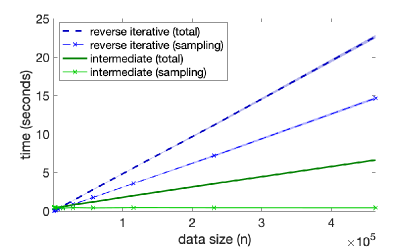
Figure 6.1: Runtime comparison of algorithms for discrete volume sampling on the MSD dataset, varying the data size $n$ by taking row subsets of the full data matrix.

For each estimator we plotted the loss $L_{\mathrm{D}}(\widehat{\mathbf{w}})$ for a range of sample sizes $k$, contrasted with the loss of the best least-squares estimator $\mathbf{w}^{*}$ computed from all data. Plots shown in Figure 6.2 were averaged over 100 runs, with shaded area representing standard error of the mean. We used six benchmark datasets from the libsvm repository (Chang and Lin, 2011), whose dimensions are given in Table 6.1.

The results confirm that our proposed leveraged volume sampling is as good or better than either of the baselines for any sample size $k$. We can see that, in some of the examples, standard volume sampling exhibits bad behavior for larger sample sizes, as suggested by the lower bound of Theorem 4.2 (especially noticeable on bodyfat and cpusmall datasets). On the other hand, leverage score sampling exhibits poor performance for small sample sizes due to the coupon collector problem, which is most noticeable for abalone dataset, where we can see a very sharp transition after which leverage score sampling becomes effective. Neither of the variants of volume sampling suffers from this issue.

Finally, in Figure 6.1, we compared the computational cost of implementing discrete volume sampling using our new distortion-free intermediate sampling (Algorithm 1) to the prior state-of-the-art method of Dereziński and Warmuth (2018), reverse iterative sampling (Algorithm 2). Note that the output samples from the two algorithms are identically distributed according to ${\mathrm{VS}_{\!\mathrm{D}_{\!\cal X}}^{d}}$, where $\mathrm{D}_{\!\cal X}$ denotes the uniform distribution over the dataset, and both of the volume sampling distributions considered in our experiments can be implemented using either of these algorithms. In the figure, we distinguished between the “total” cost and “sampling” cost: the sampling cost excludes any preprocessing steps that can be avoided during repeated sampling (see Section 1.2 for the motivations of repeated volume sampling). The preprocessing cost for both methods involves computing the leverage scores of the data matrix. The experiments were performed on MSD, the largest dataset considered in this empirical evaluation. We varied the data size by taking subsets of the full data matrix. The results were averaged over 5 runs, with the shaded area representing standard deviation. For the total cost, Figure 6.1 shows that both methods scale linearly with $n$, however our intermediate sampling approach is considerably faster for large data sizes, up to a factor of 3 in this experiment. When we look at the sampling cost, the gap between the two approaches becomes much larger because the cost of reverse iterative sampling still grows linearly with $n$, whereas the cost of intermediate sampling stays flat. As a result, for the full MSD dataset we observe at least an order of magnitude difference. This is consistent with our analysis, since Algorithm 1 effectively reduces the dataset down to an intermediate sample with size independent of $n$, and then runs reverse iterative sampling on that intermediate sample. Thus, the vast majority of the total cost of intermediate sampling involves the preprocessing step of computing the leverage scores. It is worth noting that for even larger datasets, further computational savings in the preprocessing cost can be achieved by computing the leverage scores approximately (see Section 5.4).

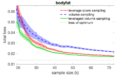
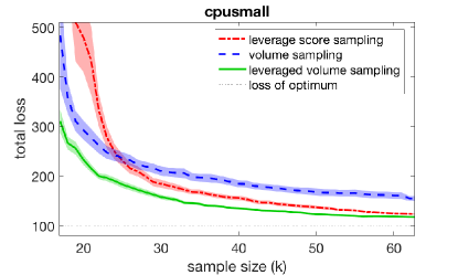
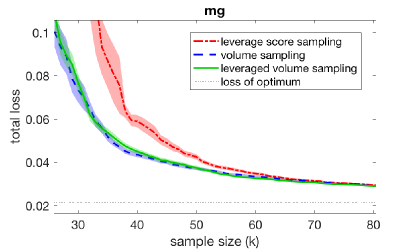
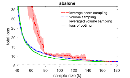
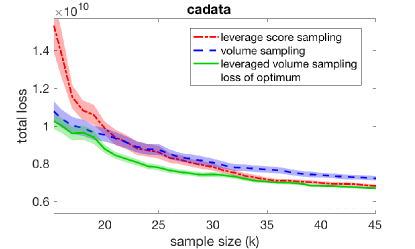
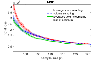
Figure 6.2: Comparison of loss of the subsampled estimator when using leveraged volume sampling vs using leverage score sampling and standard volume sampling on six datasets.

7 Conclusions

We showed that for any input distribution and $\epsilon>0$, there is a random design consisting of $O(d\log d+d/\epsilon)$ points from which an unbiased estimator can be constructed whose expected square loss over the entire distribution is bounded by $1+\epsilon$ times the loss of the optimum. However, two main open problems remain. First, can the sample size bound be reduced to $O(d/\epsilon)$? This has already been done with a biased estimator by Chen and Price (2019), but finding an unbiased estimator of the smaller size remains open.

Second, the least squares estimator combined with i.i.d. leverage score sampling already achieves loss $1+\epsilon$ times the optimum with $O(d\log d+d/\epsilon)$ points. The resulting estimator is biased. However, in our preliminary experiments the bias of exact leverage score sampling is small and decreases rather quickly (unlike for uniform sampling, or even approximate leverage score sampling, where the bias can be significant). Thus, one of the key open problems is to quantify the bias of this method.

Acknowledgments

Michał Dereziński and Manfred K. Warmuth were supported by the NSF grant IIS-1619271. Michał Dereziński would also like to thank the NSF for funding via the NSF TRIPODS program. Daniel Hsu was supported by the NSF grant CCF-1740833 and a Sloan Research Fellowship. Part of this work was done while Manfred K. Warmuth was visiting Google Inc. in Zürich and Michał Dereziński was visiting the Simons Institute for the Theory of Computing. We would also like to acknowledge Eric Price for valuable discussions regarding this paper.

A Exact calculation of $\mathbf{w}^{*}$ for the i.i.d. Gaussian experiment of the introduction and a technical proposition

Since in the setup $\boldsymbol{\Sigma}_{\mathrm{D}_{\!\cal X}}=\mathbf{I}$, the least squares solution can be computed as:

$$\mathbf{w}^{*} =\operatorname*{\mathop{\mathrm{argmin}}}_{\mathbf{w}}\mathbb{E}\big{[}(\mathbf{x}^{\scriptscriptstyle{\top}}\mathbf{w}-y)^{2}\big{]}=\boldsymbol{\Sigma}_{\mathrm{D}_{\!\cal X}}^{-1}\mathbb{E}[y\mathbf{x}]$$

$$=\sum_{i=1}^{d}\mathbb{E}\Big{[}\big{(}\tfrac{1}{3}x_{i}^{3}+x_{i}\big{)}\mathbf{x}\Big{]}=\begin{pmatrix}\mathbb{E}[\frac{1}{3}x_{1}^{4}+x_{1}^{2}]\\ |\\ \mathbb{E}[\frac{1}{3}x_{d}^{4}+x_{d}^{2}]\end{pmatrix}=\begin{pmatrix}2\\ |\\ 2\end{pmatrix}.$$

Here the second to last equality uses the fact that the cross terms are 0 due to independence and the last equality follows from the fact that $\mathbb{E}[x^{4}]=3$ and $\mathbb{E}[x^{2}]=1$, for $x\sim\mathcal{N}(0,1)$.

Proposition A.1 (Theorem 2 of Cho, 2009)

Let $\mathbf{u}=(u_{1},\dotsc,u_{d})$ be a uniformly random unit vector in $\mathbb{R}^{d}$. For any $k_{1},\dotsc,k_{d}\geq 0$,

$$\mathbb{E}\bigg{[}\prod_{j=1}^{d}|u_{j}|^{2k_{j}}\bigg{]}=\frac{\prod_{j=1}^{d}\Gamma\big{(}k_{j}+\tfrac{1}{2}\big{)}}{\Gamma\big{(}\sum_{j=1}^{d}k_{j}+\tfrac{d}{2}\big{)}}\cdot\frac{\Gamma\big{(}\tfrac{d}{2}\big{)}}{\Gamma\big{(}\tfrac{1}{2}\big{)}^{d}}.$$

B Loss bound with approximate leverage scores

In this section we describe the changes needed for the proof of Theorem 3.1 to be extended to approximate leverage score sampling, as described in Lemma 3.5. Below, we state the result in its full generality. Recall that we denote a leverage score of point $\mathbf{x}$ as $l_{\mathbf{x}}=\mathbf{x}^{\scriptscriptstyle{\top}}\boldsymbol{\Sigma}_{\mathrm{D}_{\!\cal X}}^{-1}\mathbf{x}$.

Theorem B.1

Let $\mathrm{D}_{\!\cal X}$ be a $d$-variate distribution. Assign to every $\mathbf{x}^{\scriptscriptstyle{\top}}\!\in\mathrm{supp}(\mathrm{D}_{\!\cal X})$ a real-valued $\hat{l}_{\mathbf{x}}$ such that $\frac{1}{2}l_{\mathbf{x}}\leq\hat{l}_{\mathbf{x}}\leq\frac{3}{2}l_{\mathbf{x}}$ and define the following $d$-variate distribution:

$$\mathrm{\widehat{L}ev}(A)\stackrel{{\scriptstyle\textit{\tiny{def}}}}{{=}}\frac{\mathbb{E}_{\mathrm{D}_{\!\cal X}}\big{[}\mathbf{1}_{[\mathbf{x}^{\scriptscriptstyle{\top}}\in A]}\,\hat{l}_{\mathbf{x}}\big{]}}{\mathbb{E}_{\mathrm{D}_{\!\cal X}}\big{[}\hat{l}_{\mathbf{x}}\big{]}}\quad\text{for any $\mathrm{D}_{\!\cal X}$-measurable $A$.}$$

For any $\epsilon>0$, there is $k=O(d\log d+d/\epsilon)$ such that for any $D_{{\cal Y}|\mathbf{x}}$, if we sample $\bar{\mathbf{X}}\sim{\mathrm{VS}_{\!\mathrm{D}_{\!\cal X}}^{d}}\!\cdot\mathrm{\widehat{L}ev}^{k-d}$ and $\bar{y}_{i}\sim D_{{\cal Y}|\mathbf{x}=\bar{\mathbf{x}}_{i}}$ then $\widehat{\mathbf{w}}=\operatorname*{\mathop{\mathrm{argmin}}}_{\mathbf{w}}\sum_{i=1}^{k}\frac{1}{\hat{l}_{\bar{\mathbf{x}}_{i}}}(\bar{\mathbf{x}}_{i}^{\scriptscriptstyle{\top}}\mathbf{w}-\bar{y}_{i})^{2}$ satisfies:

$$\quad\mathbb{E}[\widehat{\mathbf{w}}] =\operatorname*{\mathop{\mathrm{argmin}}}_{\mathbf{w}}L_{\mathrm{D}}(\mathbf{w})\quad\text{and}\quad\mathbb{E}\big{[}L_{\mathrm{D}}(\widehat{\mathbf{w}})\big{]}\leq(1+\epsilon)\cdot\min_{\mathbf{w}}L_{\mathrm{D}}(\mathbf{w}).$$

Proof  The reduction described at the beginning of the proof of Theorem 3.1 proceeds almost unchanged, except that now distribution $\widetilde{\mathrm{D}}$ is defined in terms of the approximate leverage scores:

$$(\widetilde{\mathbf{x}}^{\scriptscriptstyle{\top}}\!,\widetilde{y})=\bigg{(}\frac{1}{{\sqrt{{{\color[rgb]{1,1,1}|}}\!\!\smash{\text{$\hat{l}_{\widehat{\mathbf{x}}}$}}}}}\,\widehat{\mathbf{x}}^{\scriptscriptstyle{\top}}\!,\frac{1}{{\sqrt{{{\color[rgb]{1,1,1}|}}\!\!\smash{\text{$\hat{l}_{\widehat{\mathbf{x}}}$}}}}}\,\widehat{y}\bigg{)}\sim\widetilde{\mathrm{D}},$$

where $\widehat{\mathbf{x}}\sim\mathrm{\widehat{L}ev}$ and $\widehat{y}\sim D_{{\cal Y}|\mathbf{x}=\widehat{\mathbf{x}}}$. Denoting $\hat{d}=\mathbb{E}_{\mathrm{D}_{\!\cal X}}[\hat{l}_{\mathbf{x}}]\in[\frac{1}{2}d,\frac{3}{2}d]$, we have $\mathbf{\Sigma}_{{\widetilde{\mathrm{D}}_{\cal X}}}\!=\boldsymbol{\Sigma}_{\mathrm{D}_{\!\cal X}}/\hat{d}$. Also, the leverage scores of $\widetilde{\mathrm{D}}$ are approximately uniform:

$$\widetilde{\mathbf{x}}^{\scriptscriptstyle{\top}}\mathbf{\Sigma}_{{\widetilde{\mathrm{D}}_{\cal X}}}^{-1}\widetilde{\mathbf{x}}=\frac{1}{\hat{l}_{\widehat{\mathbf{x}}}}\widehat{\mathbf{x}}^{\scriptscriptstyle{\top}}\mathbf{\Sigma}_{{\widetilde{\mathrm{D}}_{\cal X}}}^{-1}\widehat{\mathbf{x}}=\frac{\hat{d}}{\hat{l}_{\widehat{\mathbf{x}}}}\widehat{\mathbf{x}}^{\scriptscriptstyle{\top}}\boldsymbol{\Sigma}_{\mathrm{D}_{\!\cal X}}^{-1}\widehat{\mathbf{x}}\,\in\,[d/3,\,3d].$$

Following the same steps as for Theorem 3.1, we conclude that without loss of generality it suffices to show the result w.r.t. loss $L_{\widetilde{\mathrm{D}}}$ for the estimator $\widetilde{\mathbf{X}}^{\dagger}\widetilde{\mathbf{y}}$ drawn from $\widetilde{\mathbf{X}}\sim{\mathrm{VS}}_{{\widetilde{\mathrm{D}}_{\cal X}}}^{d}\!\!\cdot{\widetilde{\mathrm{D}}_{\cal X}}^{k-d}$ and $\widetilde{y}_{i}\sim\widetilde{\mathrm{D}}_{{\cal Y}|\widetilde{\mathbf{x}}=\widetilde{\mathbf{x}}_{i}}$.

Using the above reduction, from now on we assume that $l_{\mathbf{x}}\in[d/3,\,3d]$ a.s. for $\mathbf{x}\sim\mathrm{D}_{\!\cal X}$, and we consider the estimator $\bar{\mathbf{X}}^{\dagger}\bar{\mathbf{y}}$, where $\bar{\mathbf{X}}\sim{\mathrm{VS}_{\!\mathrm{D}_{\!\cal X}}^{d}}\cdot\mathrm{D}_{\!\cal X}^{k-d}$. Now, the unbiasedness of this estimator follows immediately from Theorems 2.4 and 2.10. Again, without loss of generality, we can replace the distribution $\mathbf{x}^{\scriptscriptstyle{\top}}\sim\mathrm{D}_{\!\cal X}$ by the distribution of $\mathbf{x}^{\scriptscriptstyle{\top}}\boldsymbol{\Sigma}_{\mathrm{D}_{\!\cal X}}^{-\nicefrac{{1}}{{2}}}$, so from now on we will let $\boldsymbol{\Sigma}_{\mathrm{D}_{\!\cal X}}=\mathbf{I}$. The loss bound reduces to the following, same as before:

$$L_{\mathrm{D}}(\widehat{\mathbf{w}})-L_{\mathrm{D}}(\mathbf{w}^{*}) =\|\widehat{\mathbf{w}}-\mathbf{w}^{*}\|^{2}\leq\big{\|}(\bar{\mathbf{X}}^{\scriptscriptstyle{\top}}\bar{\mathbf{X}})^{-1}\|^{2}\cdot\|\bar{\mathbf{X}}^{\scriptscriptstyle{\top}}(\bar{\mathbf{y}}-\bar{\mathbf{X}}\mathbf{w}^{*})\big{\|}^{2}.$$ (B.1)

Applying Lemma 3.2 for $\mathrm{D}_{\!\cal X}$ with $K=3d$, $m=k-\lfloor k/2\rfloor$ and $\epsilon=1/2$ we obtain that if $k\geq d+12Cd\log d/\delta$ then $\bar{\mathbf{X}}\sim{\mathrm{VS}_{\!\mathrm{D}_{\!\cal X}}^{d}}\cdot\mathrm{D}_{\!\cal X}^{k-d}$ with probability at least $1-\delta$ satisfies

$$\mathcal{E}\mathrel{\mathop{\mathchar 58\relax}}\qquad\bar{\mathbf{X}}_{[s]^{c}}^{\scriptscriptstyle{\top}}\bar{\mathbf{X}}_{[s]^{c}}\succeq\frac{k}{4}\cdot\mathbf{I},\quad\text{ where }s=\lfloor k/2\rfloor.$$

We now decompose the expectation into two terms depending on whether the event $\mathcal{E}$ occurs or not:

$$\mathbb{E}[\|\widehat{\mathbf{w}}-\mathbf{w}^{*}\|^{2}]=\mathrm{Pr}(\mathcal{E})\cdot\mathbb{E}[\|\widehat{\mathbf{w}}-\mathbf{w}^{*}\|^{2}\mid\mathcal{E}]+\mathrm{Pr}(\neg\mathcal{E})\cdot\mathbb{E}[\|\widehat{\mathbf{w}}-\mathbf{w}^{*}\|^{2}\mid\neg\mathcal{E}],$$ (B.2)

and the proof is divided into two parts, for handling the two terms.

Part 1: Event $\mathcal{E}$ suceeds

We use the upper bound from (B.1). Event $\mathcal{E}$ implies that $\|(\bar{\mathbf{X}}^{\scriptscriptstyle{\top}}\bar{\mathbf{X}})^{-1}\|^{2}\leq 4^{2}/k^{2}$. The second term in (B.1) is decomposed similarly as in (3.5), however bounding each of the obtained components will require a bit more care. Denoting $\bar{\mathbf{r}}=\bar{\mathbf{y}}-\bar{\mathbf{X}}\mathbf{w}^{*}$, we have

$$\mathbb{E}\big{[}\big{\|}\bar{\mathbf{X}}^{\scriptscriptstyle{\top}}\bar{\mathbf{r}}\big{\|}^{2}\big{]} =\sum_{\{i,j\}\subseteq[d]}\!\!\mathbb{E}\big{[}\bar{r}_{i}\bar{r}_{j}\bar{\mathbf{x}}_{i}^{\scriptscriptstyle{\top}}\bar{\mathbf{x}}_{j}\big{]}+\sum_{i\in[d]}\mathbb{E}\big{[}\|\bar{\mathbf{x}}_{i}\bar{r}_{i}\|^{2}\big{]}+\sum_{i\in[d]^{c}}\mathbb{E}\big{[}\|\bar{\mathbf{x}}_{i}\bar{r}_{i}\|^{2}\big{]}$$

$$=d(d\!-\!1)\,\mathbb{E}\big{[}\bar{r}_{1}\bar{r}_{2}\bar{\mathbf{x}}_{1}^{\scriptscriptstyle{\top}}\bar{\mathbf{x}}_{2}\big{]}+d\,\mathbb{E}\big{[}\bar{r}_{1}^{2}l_{\bar{\mathbf{x}}_{1}}\big{]}+(k-d)\,\mathbb{E}_{\mathrm{D}_{\!\cal X}}\big{[}(y-\mathbf{x}^{\scriptscriptstyle{\top}}\mathbf{w}^{*})^{2}l_{\mathbf{x}}\big{]}.$$

Since $l_{\mathbf{x}}\leq 3d$, the last component above can be immediately bounded by $3d(k-d)L_{\mathrm{D}}(\mathbf{w}^{*})$. Invoking Theorem 2.7, we know that $\bar{\mathbf{x}}_{1}\sim\mathrm{Lev}_{\mathrm{D}_{\!\cal X}}$ so the second term can be bounded as follows: $d\,\mathbb{E}[\bar{r}_{1}^{2}l_{\bar{\mathbf{x}}_{1}}]=d\,\mathbb{E}_{\mathrm{D}}[(y-\mathbf{x}^{\scriptscriptstyle{\top}}\mathbf{w}^{*})l_{\mathbf{x}}^{2}]/d\leq 9d^{2}L_{\mathrm{D}}(\mathbf{w}^{*})$. The remaining term is computed by invoking Lemma 3.3. Denoting $r_{i}=y_{i}-\mathbf{x}_{i}^{\scriptscriptstyle{\top}}\mathbf{w}^{*}$, we have

$$d(d\!-\!1)\,\mathbb{E}\big{[}\bar{r}_{1}\bar{r}_{2}\bar{\mathbf{x}}_{1}^{\scriptscriptstyle{\top}}\bar{\mathbf{x}}_{2}\big{]} =d(d\!-\!1)\,\mathbb{E}_{\mathrm{D}^{2}}\big{[}r_{1}r_{2}\mathbf{x}_{1}^{\scriptscriptstyle{\top}}\mathbf{x}_{2}\cdot\big{(}l_{\mathbf{x}_{1}}l_{\mathbf{x}_{2}}\ -(\mathbf{x}_{1}^{\scriptscriptstyle{\top}}\mathbf{x}_{2})^{2}\big{)}\big{]}/d^{\underline{2}}$$

$$=\big{\|}\mathbb{E}_{\mathrm{D}}[(y-\mathbf{x}^{\scriptscriptstyle{\top}}\mathbf{w}^{*})l_{\mathbf{x}}\mathbf{x}]\big{\|}^{2}-\underbrace{\mathbb{E}_{\mathrm{D}^{2}}\big{[}r_{1}r_{2}(\mathbf{x}_{1}^{\scriptscriptstyle{\top}}\mathbf{x}_{2})^{3}\big{]}}_{\geq 0}$$

$$\overset{(*)}{\leq}\mathbb{E}_{\mathrm{D}}\big{[}(y-\mathbf{x}^{\scriptscriptstyle{\top}}\mathbf{w}^{*})l_{\mathbf{x}}^{2}\big{]}\leq 9d^{2}L_{\mathrm{D}}(\mathbf{w}^{*}),$$

where $(*)$ is implied by the following more general property of the random vector $\mathbf{x}^{\scriptscriptstyle{\top}}\sim\mathrm{D}_{\!\cal X}$ when $\boldsymbol{\Sigma}_{\mathrm{D}_{\!\cal X}}=\mathbf{I}$: for any random variable $b$ jointly distributed with $\mathbf{x}$ we have $\|\mathbb{E}[b\,\mathbf{x}]\|^{2}\leq\mathbb{E}[b^{2}]$. This follows because $\mathbb{E}[\mathbf{x}\mathbf{x}^{\scriptscriptstyle{\top}}]=\mathbf{I}$, so the components of $\mathbf{x}$, treated as scalar random variables, form an orthonormal basis of a $d$-dimensional subspace of the Hilbert space $\mathcal{H}$ of square-integrable random variables. Thus, $\|\mathbb{E}[b\mathbf{x}]\|^{2}$, which is the $\mathcal{H}$-norm of the projection of $b$ onto that subspace, is no more than the $\mathcal{H}$-norm of $b$ itself.

Part 2: Event $\mathcal{E}$ fails

This part follows identically as in the proof of Theorem 3.1, except that when applying Lemma 3.4, we use the fact that $\|\mathbf{x}\|^{2}\leq 3d$, obtaining:

$$\mathbb{E}\big{[}\mathrm{tr}((\bar{\mathbf{X}}_{[s]}\bar{\mathbf{X}}_{[s]})^{-1})\|\bar{\mathbf{r}}_{[s]}\|^{2}\big{]} \leq s\cdot\Big{(}\frac{d}{s}\cdot L_{\mathrm{D}}(\mathbf{w}^{*})+\frac{d-1}{s(s-d+1)}\cdot\mathbb{E}_{\mathrm{D}_{\!\cal X}}\big{[}\|\mathbf{x}\|^{2}\bar{r}_{1}^{2}\big{]}\Big{)}$$

$$\leq d\cdot L_{\mathrm{D}}(\mathbf{w}^{*})+\frac{3d(d-1)}{s-d+1}\cdot L_{\mathrm{D}}(\mathbf{w}^{*})\leq 10d\,L_{\mathrm{D}}(\mathbf{w}^{*}).$$

With the remaining steps same as in Theorem 3.1, this concludes the proof.  

C Volume-rescaled sampling conditioned on the covariance

In this section we present the proof of a lemma used to construct volume-rescaled samples when $\mathrm{D}_{\!\cal X}$ is a centered multivariate Gaussian distribution.

Lemma C.1 (restated Lemma 5.4)

For any $\mathbf{\Sigma}\in\mathbb{R}^{d\times d}$, the conditional distribution of $\bar{\mathbf{X}}\sim{\mathrm{VS}_{\!\mathrm{D}_{\!\cal X}}^{k}}$ given $\bar{\mathbf{X}}^{\scriptscriptstyle{\top}}\bar{\mathbf{X}}=\mathbf{\Sigma}$ is the same as the conditional distribution of $\mathbf{X}\sim\mathrm{D}_{\!\cal X}^{k}$ given $\mathbf{X}^{\scriptscriptstyle{\top}}\mathbf{X}=\mathbf{\Sigma}$.

Proof  Since we are conditioning on an event which may have probability $0$, this requires a careful limiting argument. Let $A$ be any measurable event over the random matrix $\bar{\mathbf{X}}$ and let $C_{\mathbf{\Sigma}}^{\epsilon}\stackrel{{\scriptstyle\textit{\tiny{def}}}}{{=}}\big{\{}\mathbf{B}\in\mathbb{R}^{d\times d}\,\mathrel{\mathop{\mathchar 58\relax}}\,\|\mathbf{B}-\mathbf{\Sigma}\|\leq\epsilon\big{\}}$ be an $\epsilon$-neighborhood of $\mathbf{\Sigma}$ w.r.t. the matrix $2$-norm such that $\mathrm{Pr}(\bar{\mathbf{X}}^{\scriptscriptstyle{\top}}\bar{\mathbf{X}}\!\in\!C_{\mathbf{\Sigma}}^{\epsilon}>0)$. We write the probability of $\bar{\mathbf{X}}\in A$ conditioned on $\bar{\mathbf{X}}^{\scriptscriptstyle{\top}}\bar{\mathbf{X}}\in C_{\mathbf{\Sigma}}^{\epsilon}$ as:

$$\mathrm{Pr}\big{(}\bar{\mathbf{X}}\!\in\!A\,| \,\bar{\mathbf{X}}^{\scriptscriptstyle{\top}}\bar{\mathbf{X}}\!\in\!C_{\mathbf{\Sigma}}^{\epsilon}\big{)}=\frac{\mathrm{Pr}\big{(}\bar{\mathbf{X}}\!\in\!A\,\wedge\,\bar{\mathbf{X}}^{\scriptscriptstyle{\top}}\bar{\mathbf{X}}\!\in\!C_{\mathbf{\Sigma}}^{\epsilon}\big{)}}{\mathrm{Pr}\big{(}\bar{\mathbf{X}}^{\scriptscriptstyle{\top}}\bar{\mathbf{X}}\!\in\!C_{\mathbf{\Sigma}}^{\epsilon}\big{)}}=\frac{\mathbb{E}\big{[}\mathbf{1}_{[\mathbf{X}\in A]}\mathbf{1}_{[\mathbf{X}^{\scriptscriptstyle{\top}}\mathbf{X}\in C_{\mathbf{\Sigma}}^{\epsilon}]}\det(\mathbf{X}^{\scriptscriptstyle{\top}}\mathbf{X})\big{]}}{\mathbb{E}\big{[}\mathbf{1}_{[\mathbf{X}^{\scriptscriptstyle{\top}}\mathbf{X}\in C_{\mathbf{\Sigma}}^{\epsilon}]}\det(\mathbf{X}^{\scriptscriptstyle{\top}}\mathbf{X})\big{]}}$$

$$\leq\frac{\mathbb{E}\big{[}\mathbf{1}_{[\mathbf{X}\in A]}\mathbf{1}_{[\mathbf{X}^{\scriptscriptstyle{\top}}\mathbf{X}\in C_{\mathbf{\Sigma}}^{\epsilon}]}\det(\mathbf{\Sigma})(1+\epsilon)^{d}\big{]}}{\mathbb{E}\big{[}\mathbf{1}_{[\mathbf{X}^{\scriptscriptstyle{\top}}\mathbf{X}\in C_{\mathbf{\Sigma}}^{\epsilon}]}\det(\mathbf{\Sigma})(1-\epsilon)^{d}\big{]}}=\frac{\mathbb{E}\big{[}\mathbf{1}_{[\mathbf{X}\in A]}\mathbf{1}_{[\mathbf{X}^{\scriptscriptstyle{\top}}\mathbf{X}\in C_{\mathbf{\Sigma}}^{\epsilon}]}\big{]}}{\mathbb{E}\big{[}\mathbf{1}_{[\mathbf{X}^{\scriptscriptstyle{\top}}\mathbf{X}\in C_{\mathbf{\Sigma}}^{\epsilon}]}\big{]}}\bigg{(}\frac{1+\epsilon}{1-\epsilon}\bigg{)}^{d}$$

$$=\mathrm{Pr}\big{(}\mathbf{X}\!\in\!A\,|\,\mathbf{X}^{\scriptscriptstyle{\top}}\mathbf{X}\!\in\!C_{\mathbf{\Sigma}}^{\epsilon}\big{)}\bigg{(}\frac{1+\epsilon}{1-\epsilon}\bigg{)}^{d}\overset{\epsilon\rightarrow 0}{\longrightarrow}\mathrm{Pr}\big{(}\mathbf{X}\!\in\!A\,|\,\mathbf{X}^{\scriptscriptstyle{\top}}\mathbf{X}\!=\!\mathbf{\Sigma}\big{)}.$$

We can obtain a lower-bound analogous to the above upper-bound, namely $\mathrm{Pr}\big{(}\mathbf{X}\!\in\!A\,|\,\mathbf{X}^{\scriptscriptstyle{\top}}\mathbf{X}\!\in\!C_{\mathbf{\Sigma}}^{\epsilon}\big{)}\big{(}\frac{1-\epsilon}{1+\epsilon}\big{)}^{d}$, which also converges to $\mathrm{Pr}\big{(}\mathbf{X}\!\in\!A\,|\,\mathbf{X}^{\scriptscriptstyle{\top}}\mathbf{X}\!=\!\mathbf{\Sigma}\big{)}$. Thus, we conclude that:

$$\mathrm{Pr}\big{(}\bar{\mathbf{X}}\!\in\!A\,|\,\bar{\mathbf{X}}^{\scriptscriptstyle{\top}}\bar{\mathbf{X}}\!=\!\mathbf{\Sigma}\big{)} =\lim_{\epsilon\rightarrow 0}\,\mathrm{Pr}\big{(}\bar{\mathbf{X}}\!\in\!A\,|\,\bar{\mathbf{X}}^{\scriptscriptstyle{\top}}\bar{\mathbf{X}}\!\in\!C_{\mathbf{\Sigma}}^{\epsilon}\big{)}=\mathrm{Pr}\big{(}\mathbf{X}\!\in\!A\,|\,\mathbf{X}^{\scriptscriptstyle{\top}}\mathbf{X}\!=\!\mathbf{\Sigma}\big{)},$$

completing the proof.

References

Ahlswede and Winter (2002)
Rudolf Ahlswede and Andreas Winter.
Strong converse for identification via quantum channels.
IEEE Transactions on Information Theory, 48(3):569–579, 2002.
Ailon and Chazelle (2009)
Nir Ailon and Bernard Chazelle.
The fast Johnson–Lindenstrauss transform and approximate nearest
neighbors.
SIAM Journal on computing, 39(1):302–322,
2009.
Anari and Dereziński (2020)
Nima Anari and Michał Dereziński.
Isotropy and Log-Concave Polynomials: Accelerated Sampling and
High-Precision Counting of Matroid Bases.
Proceedings of the 61st Annual Symposium on Foundations of
Computer Science, 2020.
Anari et al. (2022)
Nima Anari, Michał Dereziński, Thuy-Duong Vuong, and Elizabeth Yang.
Domain sparsification of discrete distributions using entropic
independence.
In 13th Innovations in Theoretical Computer Science Conference
(ITCS 2022), 2022.
Avron and Boutsidis (2013)
Haim Avron and Christos Boutsidis.
Faster subset selection for matrices and applications.
SIAM Journal on Matrix Analysis and Applications, 34(4):1464–1499, 2013.
Bardenet and Hardy (2020)
Rémi Bardenet and Adrien Hardy.
Monte carlo with determinantal point processes.
The Annals of Applied Probability, 30(1):368–417, 2020.
Bardenet et al. (2017)
Rémi Bardenet, Frédéric Lavancier, Xavier MARY, and Aurélien
Vasseur.
On a few statistical applications of determinantal point processes.
ESAIM: Proceedings and Surveys, 60, 2017.
Batson et al. (2012)
Joshua Batson, Daniel A Spielman, and Nikhil Srivastava.
Twice-Ramanujan sparsifiers.
SIAM Journal on Computing, 41(6):1704–1721, 2012.
Belhadji et al. (2020)
Ayoub Belhadji, Rémi Bardenet, and Pierre Chainais.
A determinantal point process for column subset selection.
Journal of Machine Learning Research, 21(197):1–62, 2020.
Ben-Tal and Teboulle (1990)
Aharon Ben-Tal and Marc Teboulle.
A geometric property of the least squares solution of linear
equations.
Linear Algebra and its Applications, 139:165 – 170,
1990.
Calandriello et al. (2020)
Daniele Calandriello, Michał Dereziński, and Michal Valko.
Sampling from a k-dpp without looking at all items.
In Advances in Neural Information Processing Systems,
volume 33, pages 6889–6899, 2020.
Chang and Lin (2011)
Chih-Chung Chang and Chih-Jen Lin.
LIBSVM: A library for support vector machines.
ACM Transactions on Intelligent Systems and Technology,
2:27:1–27:27, 2011.
Software available at http://www.csie.ntu.edu.tw/~cjlin/libsvm.
Chao and Strawderman (1972)
Min-Te Chao and WE Strawderman.
Negative moments of positive random variables.
Journal of the American Statistical Association, 67(338):429–431, 1972.
Chen and Price (2019)
Xue Chen and Eric Price.
Active regression via linear-sample sparsification.
In Proceedings of the 32nd Conference on Learning Theory,
2019.
Cho (2009)
Eungchun Cho.
Inner product of random vectors.
International Journal of Pure and Applied Mathematics,
56(2):217–221, 2009.
Dereziński (2019)