Travel Time Estimation without Road Networks: An Urban Morphological Layout Representation Approach

Abstract

Travel time estimation is a crucial task for not only personal travel scheduling but also city planning. Previous methods focus on modeling toward road segments or sub-paths, then summing up for a final prediction, which have been recently replaced by deep neural models with end-to-end training. Usually, these methods are based on explicit feature representations, including spatio-temporal features, traffic states, etc. Here, we argue that the local traffic condition is closely tied up with the land-use and built environment, i.e., metro stations, arterial roads, intersections, commercial area, residential area, and etc, yet the relation is time-varying and too complicated to model explicitly and efficiently. Thus, this paper proposes an end-to-end multi-task deep neural model, named Deep Image to Time (DeepI2T), to learn the travel time mainly from the built environment images, a.k.a. the morphological layout images, and showoff the new state-of-the-art performance on real-world datasets in two cities. Moreover, our model is designed to tackle both path-aware and path-blind scenarios in the testing phase. This work opens up new opportunities of using the publicly available morphological layout images as considerable information in multiple geography-related smart city applications.

1 Introduction

Travel time estimation in the urban area is vital to individual travel planning, transportation and city planning. Timely estimation of travel time help travelers to effectively schedule their trips in advance, plan the charging of electric vehicles Xu et al. (2018), evaluate travel exposure to air pollution Xu et al. (2019), and help transportation network companies to improve the service quality of delivery vehicles Mori et al. (2015). From transportation planning perspectives, travel time estimation can facilitate the quantification of individual driver’s contribution to the overall traffic congestion Çolak et al. (2016); Xu and González (2017). Travel time is also one of the most important metrics to evaluate residents’ accessibility to resources in city planning Weiss et al. (2018). However, travel time estimation in traffic is still challenging due to the complexity of transportation systems and the unpredictability of individual travel needs and mobility behavior, especially in urban regions.

This work places the emphasis on travel time estimation for a trip query in urban environment utilizing massive trajectory data. The developed model desires to tackle not only the path-aware query, where the routing path is available, but also the path-blind query, which provides the origin and destination locations only. Recent solutions are proposed in two aspects (i) link-based and (ii) path-based approaches. The former first individually model the travel time on each traversed link and then accumulate them for a given path. The main drawbacks of these approaches are the accumulation of error and the ignorance of travel delay at the intersections and traffic signals. Besides, they can not directly work for the path-blind travel time estimation Woodard et al. (2017). Path-based approaches aim to directly estimate the travel time of the whole path. There are two ways to preprocess the path before training models, mapping the path to road networks via map-matching Li et al. (2018), which is computationally expensive for massive trajectory data, and to grid cells Zhang et al. (2018). Regarding the gridding methods, the varying traffic states in one grid is intractable to capture as there might be multiple roads in the same grid and the traffic states on different segments and directions are dramatically divergent.

Inspired by the relation between traffic congestion and urban land use and organization Tsekeris and Geroliminis (2013); Louf and Barthelemy (2013); Lee et al. (2017), we desire to capture the congestion level of local regions from their morphological layouts. Figure 1 illustrates diverse morphological layouts in an urban area with additional traffic states in Google Maps. The layouts provide rich and learnable information about the built environments, including transportation infrastructure (levels of roads are differentiated by colors or widths), green spaces, density of buildings, commercial regions, etc. Albert et al. (2017). The variant built environments imply the nontrivial yet easy to be neglected connection between traffic congestion and the layout. Thus, appropriate representation of layout images could be a significant proxy of traffic states. The travel delay would be heavy if a driver traverses busy regions, such as the regions with dense traffic facilities (e.g., metro stations) or commercial facilities.

Figure 1: Illustrations of different morphological layouts with traffic states in urban environment, provided by Google Maps.

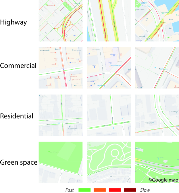
Taking cognizance of the relation between built environment and traffic congestion, in this paper, we are interested in the question ”Could we learn the travel delay from the urban layout images?” To this end, we present an end-to-end multi-task deep learning model, named Deep Image to Time (DeepI2T), to estimate the travel time of a path with the representation of layout images of the traversed grid sequence. Our main contributions are summarized as follows.

• We propose an end-to-end multi-task deep learning approach for travel time estimation by integrating the trajectory data with morphological layout images. To the best of our knowledge, this is the first time to introduce the fine-scale layout images in transportation.

• DeepI2T learns the travel delay during the whole paths and sub-paths from the gridding images, without the use of road networks, hence without map-matching.

• We combine the layout images in grids with driving direction of each vehicle. Heterogeneous traffic conditions in one single grid could be represented distinctively.

• DeepI2T could work for both path-ware and path-blind trip query in the testing stage. A neighboring trips solution is designed to tackle the path-blind query.

• We showcase DeepI2T with massive trajectory data in two cities. The performance is competitive with several state-of-the-art baselines.

2 Related Work

According to the information provided by the trip query in the testing phase, these path-based (a.k.a. trajectory-based) approaches fall into two categories, path-aware and path-blind.

Path-aware query provides the specific routing path of the trip to the estimation model. Wang et al. estimated the travel time of each road segment using tensor-based spatial-temporal model, which could handle the roads not traversed by any trajectory Wang et al. (2014). Similarly, Woodard et al. proposed to model the congestion levels on each individual segment using historical trajectory data Woodard et al. (2017). In Wang et al. (2018b), the authors formulated the travel time estimation to regression problem and proposed wide-deep-recurrent model feeding with multiple features, including the spatial, temporal, traffic, and personalized features. In these works, for modeling the traffic features on individual road segments, map-matching is a must in the primary stage and the queried trip must provide the taking route to the model (a.k.a., a sequence of road segments).

Thanks to the powerful representation ability of deep neural networks, recent works attempted to directly learn the travel time from trajectory data, without the time-consuming map-matching. Zhang et al. first mapped the GPS locations to grids and designed a model to estimate travel time by combining the spatial and temporal embedding with some auxiliary features, including the driving states, short-term and long-term traffic states in grids Zhang et al. (2018). Wang et al. designed an end-to-end framework to learn the spatial and temporal dependencies from the raw GPS sequence Wang et al. (2018a). During the testing phase, the path of the queries trip is provided as a sequence of GPS locations in a route. As this method is trained on the raw GPS coordinates, its performance is sensitive to the quality of training data and difference between training and testing data.

Path-blind query only provides the origin and destination locations and departure time to the estimation model. It’s also named as Origin-Destination (OD) travel time estimation and is universal in urban planning for the evaluation of reachability to facilities. In contrast with path-ware, path-blind query faces with great challenge due to the uncertain route and travel distance. Li et at. built a spatial and temporal graph on the map to learn the prior knowledge from the traces and designed a multi-task framework to learn the path information between origin and destination Li et al. (2018). This work models the road network as an undirected graph, which ignores the divergence of traffic states in different directions. Although not dealing with the trajectory data, Wang et al. proposed a simple baseline for the path-blind travel time estimation using only the origin and destination information in the training sets Wang et al. (2016). The idea is to find the neighboring trips for a queries trip and simply scaling their historical travel times. This method can not perform stably when less neighboring trips are available in training sets.

3 Preliminary

Driving Trajectory.

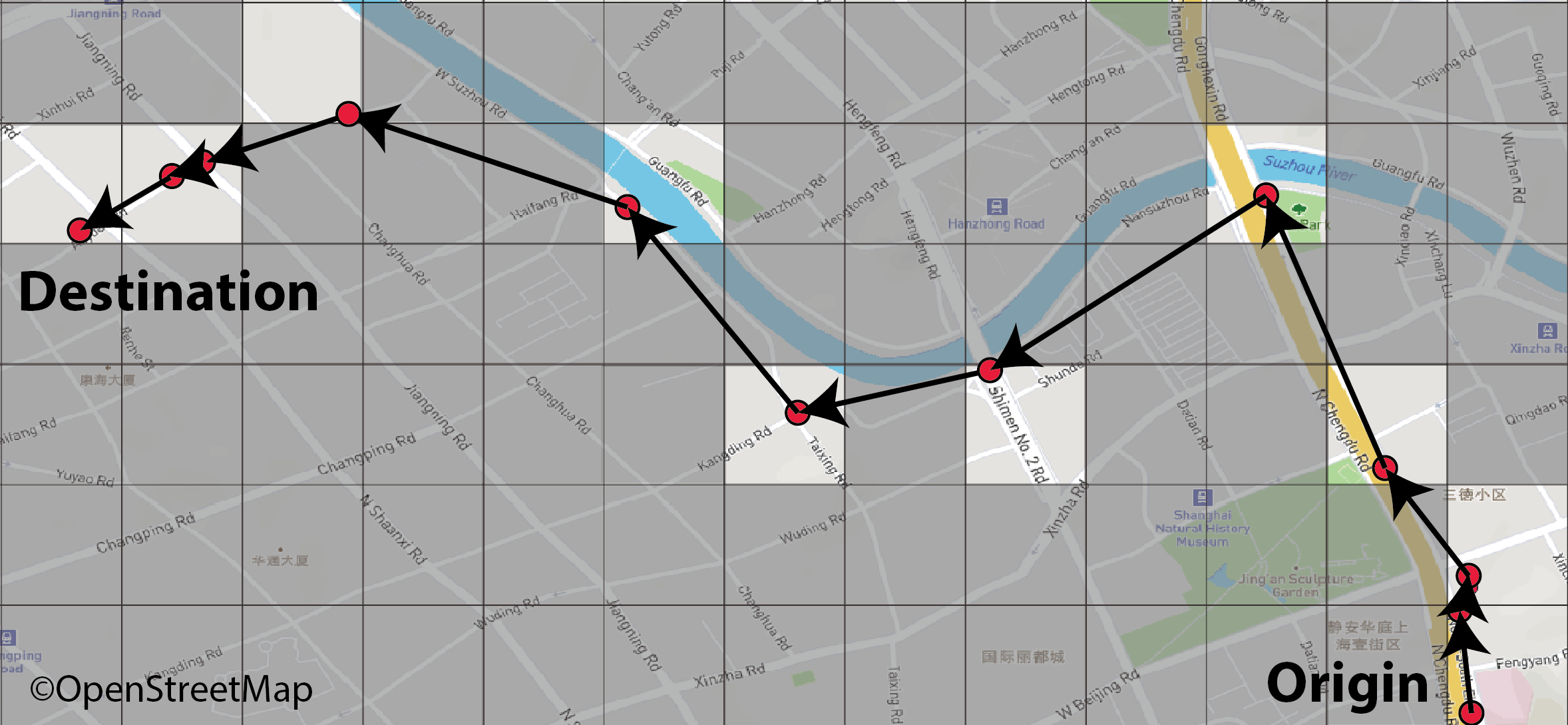
The trajectory of a driving trip, $P$, is composed of a sequence of geographical locations $\{Lon,Lat\}$ with timestamps. Each trip is associated with a vehicle ID. Therefore, a trip with $N$ footprints can be formulated as, $P=\{F_{1},F_{2},...,F_{N}\}$, where the $i$th footprint $F_{i}=(t_{i},Lon_{i},Lat_{i})$. The travel time of the path $T_{P}=t_{N}-t_{1}$. The travel distance of the trip equals to the accumulation of great-circle distances between two consecutive footprints, that is, $D=\sum_{i=1}^{N-1}Dist((Lon_{i},Lat_{i})\rightarrow(Lon_{i+1},Lat_{i+1}))$. Figure 2 illustrates a path with 12 footprints from east to west.

Figure 2: Illustrations of a trajectory and traversed grids.

Morphological Layout Images.

The study region is first divided into a number of equal-sized grids. In each grid, we crawl the high-resolutional map from the publicly available map service, OpenStreetMap OpenStreetMap (2018), using the Leaflet API Leaflet (2018). In the morphological layout images, we can visually observe different build environments, i.e., river, park, bridge, expressway, main and secondary roads. As shown in Figure 2, each point in a path could be mapped to a grid image. In this way, the path $P$ could be presented using grid images, $P^{\prime}=\{(t_{1},g_{1}),(t_{2},g_{2}),...,(t_{N},g_{N})\}$, where $g_{i}$ denotes the traversed grid image at time $t_{i}$. Note that $g_{i}$ could be repeated as multiple points might present in one grid.

4 Model Description.

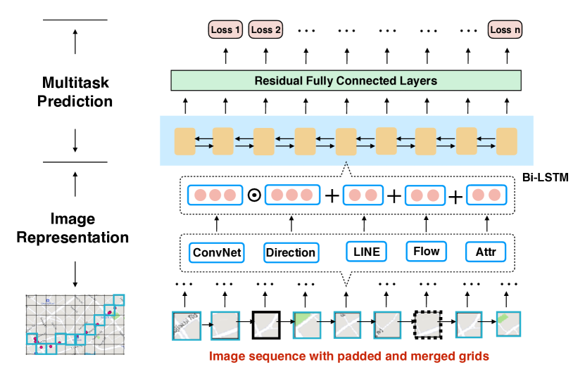
As shown in Figure 3, our proposed DeepI2T has two components: Image Representation and Multitask Prediction. The first component focuses on extracting feature patterns from morphological layout images using deep convolutional neural networks, while the second component aims at learning sequential dependency among the grids with supervision from multi-task MAPE loss.

Figure 3: Our proposed DeepI2T architecture. We merge GPS points if they share the same grid (bold frame) and pad new grids (dashed frame) if two continuous GPS points are not neighbors. $\odot$ is element-wise multiplication and $+$ is vector concatenation.

Figure 4: ConvNet architecture and direction embeddings.

4.1 Image Representation

For each grid image, we apply deep convolutional neural networks to recognize the patterns, which are twisted by direction embedding. We also consider topological information and traffic flow from all the grids, as well as some attribute information, including start time, driver ID and etc. Specifically, we have five modules: ConvNet, Direction, LINE, Flow and Attributes, which we illustrate each as follows:

ConvNet.

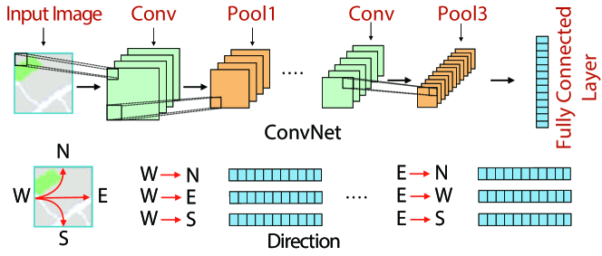
Deep convolutional neural networks Krizhevsky et al. (2012) show strong ability in capturing image patterns, e.g. arterial roads, intersections, commercial area and etc. In order to achieve this goal, we designed a 7-layer ConvNet (shown in Figure 4), containing 3 convolutional layers, 3 pooling layers, and one fully connected layer for final representation. The detailed parameters of each layer are shown in Table 1. Specifically, we conduct 2-D convolution as

$$y_{i^{l+1},j^{l+1},d^{l+1}}= \sum_{i=0}^{H}\sum_{j=0}^{W}\sum_{d^{l}=0}^{D^{l}}f_{i,j,d^{l},d^{l+1}}*x_{i^{l+1}+i,j^{l+1}+j,d^{l}}$$

$$+b_{i^{l+1},j^{l+1},d^{l+1}}$$ (1)

where $f_{i,j,d^{l},d}$ is an element from kernel vector $\bf{f}$ with size $(H,W,D^{l},D^{l+1})$, representing height $H$, width $W$, in channels $D^{l}$ and out channels $D^{l+1}$. $x_{i^{l+1}+i,j^{l+1}+j,j,d^{l}}$ refers to an element from $\bm{x^{l}}$, which is the input data at layer $l$ with size $(H^{l},W^{l},D^{l})$. The output $y_{i^{l+1},j^{l+1},d}$ is an element from $\bm{y^{l+1}}$ with size $(H^{l+1},W^{l+1},D^{l+1})$. The bias term $b_{i^{l+1},j^{l+1},d^{l+1}}$ is added into $y_{i^{l+1},j^{l+1},d^{l+1}}$. After convolution, we apply Relu function $Relu(x)=max(0,x)$ for non-linear mapping, and max pooling for down sampling. The last fully connected layer finally outputs 200-dimension vector.

	Type	Kernel size	Stride	Input size
Layer 1	Conv2D	$3*3$	$1$	$3*436*373$
Layer 2	Pooling	$2*2$	$2$	$8*436*373$
Layer 3	Conv2D	$3*3$	$1$	$8*218*187$
Layer 4	Pooling	$3*3$	$3$	$16*218*187$
Layer 5	Conv2D	$3*3$	$1$	$16*73*63$
Layer 6	Pooling	$3*3$	$3$	$8*73*63$
Layer 7	Full	$3*3$	$1$	$8*25*21$

Table 1: Parameter configurations of each layer in our ConvNet.

Direction.

We define 12 directions for each grid in Figure 4 and use lookup table $R^{12*200}$to map each direction into 200-dimension embedding, which will be updated during model training. In order to tweak the CNN image embedding, we conduct element-wise multiplication between direction embedding and ConvNet embedding, resulting in a final 200-dimension image representation.

LINE.

We construct grid network and apply network embedding to capture the spatial correlation between neighboring grids. Specifically, each grid is a node in a network and the neighborhood relationship is converted into edge connection, while the weight on each edge is the reciprocal of Manhattan distance between two grids. In order to simplify the network, we consider at most 5-hop neighbors, which means any two grids that are more than 5 hops away will be disconnected. The spatial locality is actually implied by the network structure, which is represented by LINE Tang et al. (2015) in our work. In addition, we use 100-dimension for this structure representation and keep updated during model training.

Flow.

The same region may have different traffic conditions as time changes, therefore we need time-varying representation for each grid. To this end, we average the number of vehicle per grid per hour. Each grid is associated with a flow vector with 24 elements, representing the change of traffic conditions every hour. Taking 100 vehicles as minimum unit, we have flow embedding as $R^{1000*50}$.

Attributes.

We consider three attribute information to improve the grid image representation: start time of the trip, vehicle ID and weather. In detail, we have three embedding lookup tables to represent each attribute: (i) we take one minute as minimum unit, given 7 days per week, we have start time embedding as $R^{10080*30}$; (ii) different drivers may have different driving habits, we encode the driver ID as $R^{25000*10}$; (iii) the weather condition is also critical for travel time estimation, we encode all kinds of weather into $R^{400*10}$.

Finally, we get 50-dimension attribute vector after concatenation. Combined with 200-dimension image representation, 100-dimension LINE representation and 50-dimension flow representation, we generate 400-dimension vector per grid.

4.2 Multitask Prediction

Following previous works Wang et al. (2018a); Zhang et al. (2018), we use Bi-LSTM Hochreiter and Schmidhuber (1997) to model sequential dependency and adopt residual connected layers for non-linear mapping. As for the prediction layer, we designed a different multitask structure, where each task is to estimate the travel time from origin grid to the current grid, to leverage the valuable information of sub-paths.

Multitask Loss Function.

Given a trip with L grids, $\{g_{1},g_{2},\ldots,g_{L}\}$, we consider not only the mean absolute percentage error (MAPE) of the whole path from $g_{1}$ to $g_{L}$, but also the MAPE of sub-paths from $g_{1}$ to $g_{l}$. To this end, the final loss $\mathcal{L}$ is defined as

where $T_{l}=t_{l}-t_{1}$ denotes the travel time from grid $g_{1}$ to $g_{l}$ and $\hat{T}_{l}$ denotes its estimation; $w_{l}$ is the predefined weight, $w_{l}=2l/(L^{2}+L-2)$, where $1<l\leq L$ and $\sum_{l=2}^{L}w_{l}=1$. In this way, we emphasize the longer sub-trips, to make sure model put more effort on whole trip estimation.

4.3 Travel Time Estimation

Path-aware Estimation.

Given a path-aware query, we map its path into grid sequence with driving directions. We then feed the grid sequence and the associated attribute information into the well-trained DeepI2T, which outputs whole travel time prediction.

Path-blind Estimation.

We design a neighboring strategy to tackle the path-blind query. Given a query with departure time, origin and destination locations, we first find the trips with the same origin and destination grids in the historical trips, namely neighboring trips. We predict the neighboring trips’ travel time at the same departure date and time as the queried trip. Finally, the travel time of queried trip is estimated by weighting the (estimated) travel time of neighboring trips with their $\ell_{1}$ distances.

where $N_{e}$ denotes the number of neighboring trips in the training set having the same origin and destination grids as, or in the neighboring grids of, the queried trip; $L_{test}$ and $L_{i}$ refer to the $\ell_{1}$ distances of the testing and neighboring trips, respectively; $\hat{T}_{test}$ and $\hat{T}_{i}$ refer to the estimated travel time of the testing and neighboring trips, respectively.

5 Experiments

5.1 Data Description

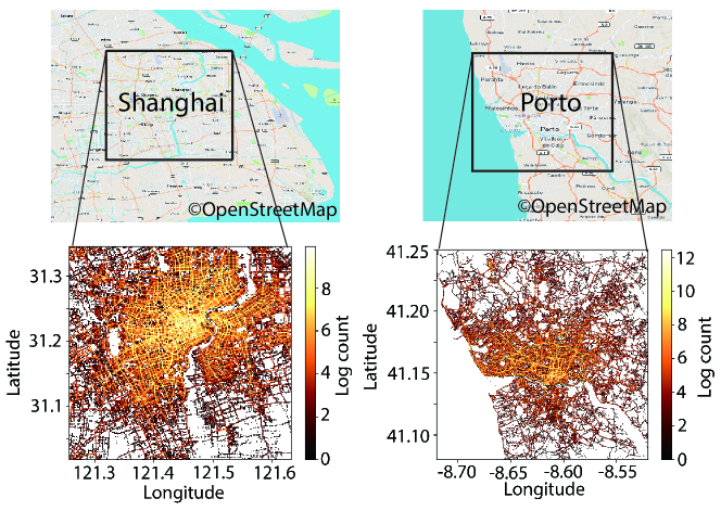
In the experiments, large-scale datasets in two cities from different countries are adopted to validate the proposed DeepI2T. The study area and the distribution of raw GPS data are presented in Figure 5. The statistical information of the datasets is shown in Table  2.

Shanghai Data.

Shanghai Data contains of the GPS trajectories of taxis from Apr. 1st to Jun. 15th in 2014, with sample interval ranges from 20s to 100s. We only keep the trips of taxis when they are transporting passengers. We select the data from Apr. 1st to May 31st for model training, and the remaining for testing.

Porto Data.

The dataset is collected from 442 taxis running in the city of Porto, Portugal, from 1st Jul. 2013 to 30th Jun. 2014, and is publicly available Taxi-Link (2018). The measurement interval of the track points is fixed at 15s in the raw data. We select the data during the first 9 months for model training, and the remaining for testing.

Figure 5: Study region and spatial distribution of GPS footprints in Shanghai in one week (left) and Porto in one year (right).

Dataset	Shanghai	Porto
area of study region	1479.7$km^{2}$	419.0$km^{2}$
# grids (W$\times$H)	200 $\times$ 175	100 $\times$ 85
size of grid	$\sim 200m$	$\sim 200m$
# vehicles	$15,000$	$442$
# trips per day	$170,000$	$3,530$
average sample rate	$55s$	$15s$
average travel time	$719s$	$749s$
travel time std	$469s$	$593s$
average travel distance	$4.53km$	$5.79km$
# days for training	61	273
# days for testing	15	90

Table 2: The statistical information of the datasets

5.2 Methods for Comparison

Linear regression (LR).

Given the geographical positions of the origin and destination, we train the relation between the $\ell_{1}$ distance and travel time using a linear regression model.

Neighbor average (AVG).

For each trip in the training data sets, the average speed is calculated with the travel time and the $\ell_{1}$ distance between the origin and destination. During the testing phase, we estimate the travel speed by simply averaging the historical speeds of its neighbors, i.e., trips between the same origin and destination grids.

Temporally weighted neighbors (TEMP).

Wang et al. proposed a simple baseline method to estimate trip travel time by scaling the average speeds of its neighboring trips Wang et al. (2016). The scaling factors are calculated by the temporal change of the average speeds of all trips in the city, i.e., relative temporal speed reference in Wang et al. (2016). Comparing with AVG method, TEMP inspects the variance in average speeds of historical trips by their departure hours.

Gradient Boosting Machine (GBM).

Gradient boosting decision tree models have been used in travel time prediction Zhang and Haghani (2015). Several attributes of trips are fed into GBM model, including the departure time, the day in a week, the geographical coordinates of the origin and destination, and the $\ell_{1}$ distance, etc. The model is implemented using LightGBM Ke et al. (2017), configured with 500 trees with 1,000 leaves.

DeepTTE.

It is a state-of-the-art end-to-end deep learning method for travel time estimation, learning the spatial and temporal dependencies of the raw GPS points in trajectories Wang et al. (2018a). We use the code shared by authors to test our two datasets. However, we find DeepTTE tends to overfit when fed with uniformly sampled GPS trajectories (i.e., Porto data has fixed sample rate). In such case, DeepTTE simply learns the travel time by counting the number of points in one trace and fails in the testing. To fix it, we feed DeepTTE with the centroids of the grids traversed by trips for both training and testing data, as same as DeepI2T.

GridLSTM.

It is a degeneration of DeepI2T by removing ConvNet and direction embedding. It learns the travel time with the spatial and temporal relation of grids in one trace.

5.3 Performance Evaluation

We utilize three metrics to evaluate the performance of reference models, mean absolute error (MAE), mean absolute percentage error (MAPE), and satisfaction rate (SR). SR is defined as the fraction of trips which estimation error rates are not more than $10\%$ and higher SR indicates better performance. The formulas of these metrics are given as follow.

where $T_{i}$ and $\hat{T}_{i}$ are the actual and estimated travel time of the $i$th trip in the $N$ testing trips.

In Table 3, we present the estimation errors of reference methods. The first group of methods (LR, AVG, GBM and TEMP) are designed for path-blind query and the second group of methods (DeepTTE and GridLSTM) are designed for path-aware query. The best performance is highlighted per metric per group. As we can see, DeepI2T performs best in both groups in terms of MAPE. Compared with GridLSTM, the introducing of image representation promotes the MAPE of path-aware queries by $10\%$ and $7\%$ in Shanghai and Porto, respectively. Regarding the path-blind queries, DeepI2T shows competitive performance with TEMP in Shanghai, but evidently better performance in Porto.

Method		Shanghai				Porto
		MAE (s)	MAPE (%)	SR (%)		MAE (s)	MAPE (%)	SR (%)
LR		186.5	27.64	23.87		287.9	49.02	17.20
AVG		158.9	22.30	29.35		235.86	30.43	24.65
GBM		144.3	22.55	30.45		238.17	37.83	22.97
TEMP Wang et al. (2016)		141.0	21.93	31.24		231.10	29.84	25.67
DeepTTE Wang et al. (2018a)		147.61	19.02	31.13		167.94	20.44	32.34
GridLSTM		117.12	16.98	37.00		139.55	18.10	38.45
DeepI2T (path-blind)		143.61	20.47	30.62		186.65	25.28	30.08
DeepI2T (path-aware)		105.43	15.20	42.23		128.26	17.08	38.97

Table 3: Overall performance comparison on Shanghai and Porto Data. Path-aware methods are highlighted in gray shadow.

Method		MAPEpeak (%)			SRpeak (%)
		AM	PM		AM	PM
LR		27.89	26.17		22.61	24.15
AVG		23.72	21.77		26.39	28.30
GBM		23.74	24.13		29.38	28.62
TEMP		23.03	23.45		30.23	29.44
DeepTTE		21.58	20.15		26.72	29.08
GridLSTM		18.95	17.95		33.40	34.62
DeepI2T (path-blind)		22.55	20.40		27.29	29.52
DeepI2T (path-aware)		16.89	15.75		37.28	41.37

Table 4: Peak hour performance comparison on Shanghai Data

We also summarize the MAPE and SR of each model during the morning (7:00-9:00) and evening (16:00-18:00) peak hours in Shanghai in Table 4. Comparing with the other two deep learning baselines, DeepI2T yields the best performance in terms of MAPE and SR on path-aware queries during both peaks. Especially during the evening peak, the SR of DeepI2T reaches $41.37\%$, while DeepTTE and GridLSTM only can achieve $29.08\%$ and $34.62\%$, respectively. That indicates DeepI2T could provide acceptable time estimation for a large fraction of trip queries during traffic congestion. The path-blind estimation also reaches competitive performance with the baselines during peak hours, except the SR during morning peak is weaker than TEMP.

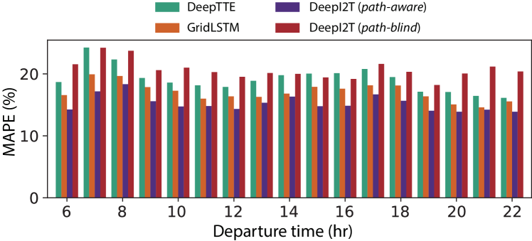
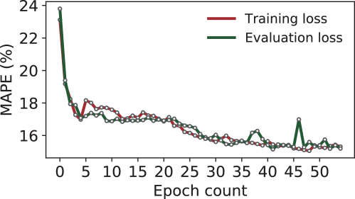
Further, we compare the performance of DeepTTE, GridLSTM and DeepI2T on Shanghai Data. Figure 6 presents the estimation error per hour. All models show relatively weak performance during the peak hours due to the traffic congestion. Even so, DeepI2T generates better estimation than compared models during all the day. In Figure 7, we compare the performance of these models per the actual travel time of queried trips. We find DeepTTE performs worse for longer trips, while the proposed DeepI2T has much stable performance for trips with varying travel time. In addition, we present the evolution of estimation error during the model training phase in Figure 8. Overall, the MAPE decays stably along with the training time. The closeness between training and evaluation curves reflects that DeepI2T efficiently prevent overfitting during model training.

Figure 6: Estimation error for trips with different departure time.

Figure 7: Estimation error for trips with different travel time. The right y-axis shows the distribution of testing trips.

Figure 8: Evolution of estimation error during model training.

It’s noteworthy that the performance of DeepTTE on our datasets is evidently weaker than the results in Wang et al. (2018a)in terms of MAPE. We argue the reasons are mainly in several aspects, (i) DeepTTE learns the dependency between two consecutive locations with their time gaps. It tends to fail when the sample rate of data is (nearly) constant; To fix this issue, we resample GPS points by using the centroids of grids. However, the time gap between two centroids may introduce some errors; (ii) DeepTTE is sensitive to the distance gap in the testing trip, which determines the similarity between testing and training data. How to select the best distance gap is not given in Wang et al. (2018a); (iii) The trip lengths in Wang et al. (2018a) are approximately twice of ours on average. Normally, for a shorter trip, the MAPE tends to be higher than longer trip even they have similar MAE. Another state-of-the-art model is DeepTravel Zhang et al. (2018), which we didn’t compare because the source code is not publicly available. We notice that the standard deviation of travel time for Porto Data in DeepTravel in Zhang et al. (2018) is much smaller than ours ($348s$ vs. $593s$), indicating the task in our work is more challenging.

6 Conclusions

This work explores the potential of learning travel delay from urban layout images for a specific task, travel time estimation. Our proposed DeepI2T model showed promising performance for both path-aware and path-blind scenarios on real-world datasets in Shanghai and Porto. Our attempt presents new opportunities of using publicly available morphological images to solve transportation problems.

References

- Albert et al. [2017] Adrian Albert, Jasleen Kaur, and Marta C Gonzalez. Using convolutional networks and satellite imagery to identify patterns in urban environments at a large scale. In Proceedings of the 23rd ACM SIGKDD International Conference on Knowledge Discovery and Data Mining, pages 1357–1366. ACM, 2017.
- Çolak et al. [2016] Serdar Çolak, Antonio Lima, and Marta C González. Understanding congested travel in urban areas. Nature Communications, 7:10793, 2016.
- Hochreiter and Schmidhuber [1997] Sepp Hochreiter and Jürgen Schmidhuber. Long short-term memory. Neural computation, 9(8):1735–1780, 1997.
- Ke et al. [2017] Guolin Ke, Qi Meng, Thomas Finley, Taifeng Wang, Wei Chen, Weidong Ma, Qiwei Ye, and Tie-Yan Liu. Lightgbm: A highly efficient gradient boosting decision tree. In Advances in Neural Information Processing Systems, pages 3146–3154, 2017.
- Krizhevsky et al. [2012] Alex Krizhevsky, Ilya Sutskever, and Geoffrey E Hinton. Imagenet classification with deep convolutional neural networks. In Advances in neural information processing systems, pages 1097–1105, 2012.
- Leaflet [2018] Leaflet. Leaflet - a JavaScript library for interactive maps. https://leafletjs.com, 2018. [Accessed Sep.-2018].
- Lee et al. [2017] Minjin Lee, Hugo Barbosa, Hyejin Youn, Petter Holme, and Gourab Ghoshal. Morphology of travel routes and the organization of cities. Nature Communications, 8(1):2229, 2017.
- Li et al. [2018] Yaguang Li, Kun Fu, Zheng Wang, Cyrus Shahabi, Jieping Ye, and Yan Liu. Multi-task representation learning for travel time estimation. In Proceedings of the 24th ACM SIGKDD International Conference on Knowledge Discovery and Data Mining, pages 1695–1704. ACM, 2018.
- Louf and Barthelemy [2013] Rémi Louf and Marc Barthelemy. Modeling the polycentric transition of cities. Physical Review Letters, 111(19):198702, 2013.
- Mori et al. [2015] Usue Mori, Alexander Mendiburu, Maite Álvarez, and Jose A Lozano. A review of travel time estimation and forecasting for advanced traveller information systems. Transportmetrica A: Transport Science, 11(2):119–157, 2015.
- OpenStreetMap [2018] OpenStreetMap. https://www.openstreetmap.org, 2018. [Accessed Sep.-2018].
- Tang et al. [2015] Jian Tang, Meng Qu, Mingzhe Wang, Ming Zhang, Jun Yan, and Qiaozhu Mei. Line: Large-scale information network embedding. In WWW. ACM, 2015.
- Taxi-Link [2018] Taxi-Link. Porto Taxi Dataset. http://www.geolink.pt/ecmlpkdd2015-challenge/dataset.html, 2018. [Accessed Oct.-2018].
- Tsekeris and Geroliminis [2013] Theodore Tsekeris and Nikolas Geroliminis. City size, network structure and traffic congestion. Journal of Urban Economics, 76:1–14, 2013.
- Wang et al. [2014] Yilun Wang, Yu Zheng, and Yexiang Xue. Travel time estimation of a path using sparse trajectories. In Proceedings of the 20th ACM SIGKDD International Conference on Knowledge Discovery and Data Mining, pages 25–34. ACM, 2014.
- Wang et al. [2016] Hongjian Wang, Yu-Hsuan Kuo, Daniel Kifer, and Zhenhui Li. A simple baseline for travel time estimation using large-scale trip data. In Proceedings of the 24th ACM SIGSPATIAL International Conference on Advances in Geographic Information Systems, page 61. ACM, 2016.
- Wang et al. [2018a] Dong Wang, Junbo Zhang, Wei Cao, Jian Li, and Yu Zheng. When will you arrive? estimating travel time based on deep neural networks. In Proceedings of the 32nd AAAI Conference on Artificial Intelligence, pages 2500–2507. AAAI, 2018.
- Wang et al. [2018b] Zheng Wang, Kun Fu, and Jieping Ye. Learning to estimate the travel time. In Proceedings of the 24th ACM SIGKDD International Conference on Knowledge Discovery and Data Mining, pages 858–866. ACM, 2018.
- Weiss et al. [2018] D. J. Weiss, A. Nelson, H. S. Gibson, W. Temperley, S. Peedell, A. Lieber, M. Hancher, E. Poyart, S. Belchior, N. Fullman, et al. A global map of travel time to cities to assess inequalities in accessibility in 2015. Nature, 553(7688):333, 2018.
- Woodard et al. [2017] Dawn Woodard, Galina Nogin, Paul Koch, David Racz, Moises Goldszmidt, and Eric Horvitz. Predicting travel time reliability using mobile phone gps data. Transportation Research Part C: Emerging Technologies, 75:30–44, 2017.
- Xu and González [2017] Yanyan Xu and Marta C González. Collective benefits in traffic during mega events via the use of information technologies. Journal of The Royal Society Interface, 14(129):20161041, 2017.
- Xu et al. [2018] Yanyan Xu, Serdar Çolak, Emre C Kara, Scott J Moura, and Marta C González. Planning for electric vehicle needs by coupling charging profiles with urban mobility. Nature Energy, 3:484–493, 2018.
- Xu et al. [2019] Yanyan Xu, Shan Jiang, Ruiqi Li, Jiang Zhang, Jinhua Zhao, Sofiane Abbar, and Marta C González. Unraveling environmental justice in ambient PM2.5 exposure in Beijing: A big data approach. Computers, Environment and Urban Systems, 75:12–21, 2019.
- Zhang and Haghani [2015] Yanru Zhang and Ali Haghani. A gradient boosting method to improve travel time prediction. Transportation Research Part C: Emerging Technologies, 58:308–324, 2015.
- Zhang et al. [2018] Hanyuan Zhang, Hao Wu, Weiwei Sun, and Baihua Zheng. DeepTravel: a neural network based travel time estimation model with auxiliary supervision. In Proceedings of the 27th International Joint Conference on Artificial Intelligence, pages 3655–3661. IJCAI, 2018.