corollarytheorem \aliascntresetthecorollary \newaliascntdefinitiontheorem \aliascntresetthedefinition \newaliascntproptheorem \aliascntresettheprop \newaliascntlemmatheorem \aliascntresetthelemma \newaliascntexampletheorem \aliascntresettheexample \newaliascntremarktheorem \aliascntresettheremark \newaliascntnotationtheorem \aliascntresetthenotation
Copula & Marginal Flows:
Disentangling the Marginal from its Joint
Abstract
Deep generative networks such as GANs and normalizing flows flourish in the context of high-dimensional tasks such as image generation. However, so far an exact modeling or extrapolation of distributional properties such as the tail asymptotics generated by a generative network is not available. In this paper we address this issue for the first time in the deep learning literature by making two novel contributions. First, we derive upper bounds for the tails that can be expressed by a generative network and demonstrate -space related properties. There we show specifically that in various situations an optimal generative network does not exist. Second, we introduce and propose copula and marginal generative flows (CM flows) which allow for an exact modeling of the tail and any prior assumption on the CDF up to an approximation of the uniform distribution. Our numerical results support the use of CM flows.
1 Introduction
Generative modeling is a major area in machine learning that studies the problem of estimating the distribution of a -valued random variable . One of the central areas of research in generative modeling is the model’s (universal) applicability to different domains, i.e. whether the distribution of can be expressed by the generative model. Generative networks, such as generative adversarial networks (GANs) [13] and normalizing flows [9, 23], comprise a relatively new class of unsupervised learning algorithms that are employed to learn the underlying distribution of by mapping an -valued independent and identically distributed (i.i.d.) random variable through a parameterized generator to the support of the targeted distribution . Due to their astonishing results in numerous scientific fields - in particular image generation [6, 20] - generative networks are generally considered to be able to model complex high-dimensional probability distributions that may lie on a manifold [2]. This lets generative networks appear to be universally applicable generative models. We claim that this impression is misleading.
In this paper we investigate to what extent this universal applicability is violated when dealing with distributions of random variables. Specifically we study the tail asymptotics generated by a generative network and the exact modeling of the tail. The right tail of is defined for and as
Similarly, the left tail is given by . The right tail function thus represents the probability that the random variable is greater than .
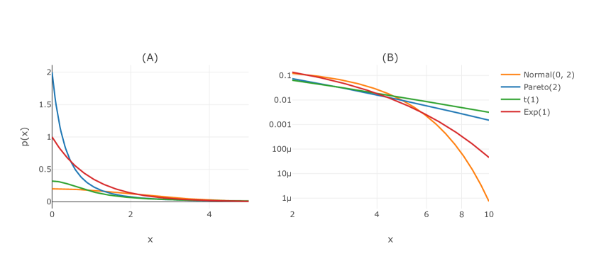
In various applications [11, 17, 22, 24] it is essential to find a generative network that satisfies
| (1) |
for all and , since the asymptotic behavior determines the propensity to generate extremal values (see Figure 1 for a comparison of the densities on the linear and logarithmic scale).111Although formally one should write we abbreviate our notation as used above.
A typical situation that appears in practice is that only a sample of is available and for and the statistician would like the generative network to fulfill a tail belief
| (2) |
which may be derived by applying methods from extreme value theory [7]. To the present moment no techniques exist in order to incorporate and model (1) or (2); thus questioning the universal applicability of generative networks to domains where an extrapolation is necessary. Although one might resort to the universal approximation theorem for MLPs [15] this is not applicable in practice as only a small proportion of the sample is found to be “in the tail”. Thus the tail cannot be learned and has to be extrapolated; whenever extrapolation is a central demand.
2 Main Results
In this paper we address the issue of modeling exact distributional properties in the sense of (1) and (2) for the first-time in the context of generative networks. Our main results can be split into two parts.
2.1 Tail Asymptotics of Generative Networks
In the first part we demonstrate that a generative network fulfilling (1) does not necessarily exist. In particular we prove the following statement:
Theorem 1.
Let be a parametrized generative network with Lipschitz constant with respect to the -norm222We define the -norm for the vector space as .. Furthermore, for set . Then the generated tail asymptotics satisfy for
The proof of Theorem 1 is provided in section 4. Theorem 1 gives rise to major implications such as the non-existence of an optimal generative network in various settings. Moreover, the result displays that the conception of choosing the noise prior is negligible is false.
In accordance to the derived tail bound the following -space333An -valued random variable is an element of the space if the expectation of with respect to some norm on is finite. related property will be proven:
Proposition \theprop.
Let and be a parametrized generative network. If is an element of , then .
The statement particularly demonstrates that a -th unbounded moment cannot be generated when inferring a noise prior where the -th moment is bounded. Finally, we conclude the section on tail bounds by observing that an exact modeling of the tails is not favored by utilizing generative networks.
2.2 Copula and Marginal Flows
In the second part we introduce and propose the use of copula and marginal generative flows (CM flows) in order to model exact tail beliefs whilst having a tractable log-likelihood. CM flows are a new model developed in this paper and are inspired by representing the joint distribution of as a copula plus its marginals, also known as a pair-copula construction (PCC) (cf. [1, 18]):
where is the density of a copula.
Following this decomposition CM flows are explicitly constructed by composing a copula flow with a marginal flow . The marginal flow approximates the inverse CDFs , whereas the copula flow approximates the generating function of . Thus, a CM flow is given by for and the used transformations are depicted in Figure 3. Although we restrict ourselves to introducing the bivariate CM flow, the proposed flow can be generalized by using Vine copulas [5, 18].
2.3 Structure
In section 4 we derive upper bounds for the tails generated by a generative network. Afterward, we introduce in section 5 CM flows in order to model exact tails. Numerical results that support the application of copula flows will be presented in section 6. Section 3 provides a literature overview and section 7 concludes this paper.
3 Related Work
PCCs were used in past works such as Copula Bayesian Networks (CBNs) [10]. CBNs marry Bayesian networks with a copula-based re-parametrization that allow for a high-dimensional representation of the multivariate targeted density. However, since CBNs are defined through a space of copula and marginal densities they can only express joint-distributions defined in within their parametric space. Despite the amount of research that was committed in defining new families of copulas that are unsymmetrical and parameterizable it is still an active area of research. With CM flows we try to learn and represent the copula by optimizing a copula flow instead of dedicating a (restricted) parametric class as in CBNs. Therefore, our approach has more flexibility, however, comes at the cost of needing to approximate uniform marginals arbitrarily well.
CM flows build up on the success of bijective neural networks by utilizing and modifying them. Therefore, our work relates in general to generative flows [8, 9, 16]. However, in this paper we discuss for the first time an exact modeling of distributional properties such as the tail of the targeted random variable.
4 Upper Tail Bounds for Generative Networks
In this section we derive an upper bound for the tail induced as well as a -space related property when feeding in the noise prior into a generative network. Prior to proving these results we introduce our setup.
4.1 Setup
We begin by defining basic but important concepts which we believe to be a subset of the general assumptions in deep learning literature. Roughly speaking, neural networks are constructed by composing affine transformations with activation functions (cf. Appendix B in Appendix B). The main property that these networks have in general is that they are Lipschitz continuous. This is done for a good reason: gradients become bounded. We therefore define a network the following way:
Definition \thedefinition (Network).
Let and be a real vector space. A function that is Lipschitz continuous is called a network. is called the parameter space. The space of networks mapping from to will be denoted by .
In the context of generative modeling we call a network a generative network when it is defined as mapping from the latent space to the data/target space for . Furthermore, a -valued random variable with i.i.d. components is called noise prior and will be denoted by throughout this section. The goal of generative modeling in the context of deep learning is to optimize the parameters of a generative network such that , is equal in distribution to . This motivates our next definition.
Definition \thedefinition (Set of Optimal Generative Networks).
Let be a noise prior and an -valued random variable. We denote by
| (3) |
where represents equality in distribution, the set of optimal generators.
Generative networks by definition can represent any affine transformation. In subsection 4.2 it will be useful to define the concept of affine lighter-tailedness in order to compare the tails that can be generated by a network with other tails.
Definition \thedefinition (Affinely Lighter-Tailed).
Let and be two -valued random variables. We call affinely lighter tailed than iff for any affine function
4.2 Results and Derivations
In what follows we demonstrate that the tail generated by a network when inducing a noise prior has order where is an affine transformation that depends on . Prior to proving our main result Theorem 1 we show in subsection 4.2 that the tail , where similarly has order as . A proof of the statement can be found in Appendix A.
Lemma \thelemma.
Let . Then for all we obtain
Next, we prove Theorem 1 by applying subsection 4.2 and utilizing Lipschitz continuity of networks.
Proof of Theorem 1.
First observe that due to the Lipschitz continuity of a generative network the following property holds for all and :
| (4) |
By applying (4) and resorting to subsection 4.2 we obtain for all
where is the first component of the random variable . From this bound the order is a direct consequence and we can conclude the statement. ∎
Theorem 1 has some immediate consequences. First, it shows that the tails of the distribution induced by the generator decay at least at the rate of an affine transformation of . Therefore, if is not affinely lighter-tailed than for some the set of optimal generative networks is empty:
Corollary \thecorollary.
Assume that for some the random variable is not affinely lighter-tailed than . Then .
The following two examples illustrate the effects of subsection 4.2 in two situations that are relevant both from a practical and theoretical perspective.
Example \theexample.
Assume is standard normally distributed and an -valued Laplace distributed random variable. Then by subsection 4.2 the set of optimal generative networks is empty.
Example \theexample.
Assume is uniformly distributed and a random variable with support . Then is bounded and again by subsection 4.2 we obtain .
Since the tail determines the probability mass allocated to extremal values it relates to the integrability of a random variable. We therefore arrive at subsection 2.1 which can be viewed as an -space related characterization of the distribution induced by . The result can be seen as another consequence of Theorem 1, but will be proven for simplicity by applying the binomial theorem.
Proof of subsection 2.1.
4.3 The Inability of Estimating and Adjusting the Tailedness
In order to estimate and consequently adjust the tail by exchanging the noise prior we would need besides the Lipschitz constant for all a “lower” Lipschitz constant which is defined for as
| (6) |
With (6) and Theorem 1 a lower and upper bound of could be obtained. However, since in general is not available we arrive at the result that the induced tail remains unknown and thus, the statistician unpleased.444We note that in simplified network constructions such as in a ReLU network the exact tail can be obtained for one-dimensional targeted random variables by using [3, Lemma 1] which shows that the domain of can be divided into a finite number of convex pieces on which is affine.
5 Copula and Marginal Flows: Model Definition
The previous section on tail bounds demonstrates that generative networks do not favor controlling the generated tail behavior. We now show how a tail belief can be incorporated by using a bivariate CM flow that is defined for as the composition of a parametrized marginal and a copula flow
The bivariate marginal flow is represented by two DDSFs (cf. [16] or Appendix B), whereas the bivariate copula flow by a 2-dimensional Real NVP [9]. Although only the bivariate case is introduced we remark that CM flows can be generalized to higher dimensions by following a Vine copula and leave this as future work. Throughout this section we assume that is -valued and are invertible.
5.1 Marginal Flows: Exact Modeling of the Tail
In what follows we construct univariate marginal flows for the -valued random variable and then define the vector-valued extension for . Beforehand let us specify the concept of tail beliefs.
Definition \thedefinition (Tail Belief).
Let and set . Furthermore, let be an -valued random variable and a known CDF. We call the tuple tail belief when we assume that
Thus, when incorporating a tail belief into a generative network we are interested in finding a mapping for that satisfies
| (7) |
In order to satisfy (7) we propose the following construction.
Definition \thedefinition (Univariate Marginal Flow).
Let and . Furthermore, let be a DDSF (cf. Appendix B) and a scaled version of which is defined as
We call a function defined as
| (8) |
a univariate marginal flow.
Properties
By construction a parametrized univariate marginal flow defines a bijection and satisfies the tail objective (7). Furthermore, the construction can be generalized in order to incorporate any prior knowledge of on a union of compact intervals. While defines an optimal map on , the flow approximates the inverse CDF on and therefore only needs to be trained on the interval .
Bivariate Marginal Flows
Generalizing univariate marginal flows to bivariate (or multivariate) marginal flows is simple. For this we assume that for we have a tail belief . Then for each we can define an univariate marginal flow and construct the multivariate marginal flow which is defined for as
5.2 Copula Flows: Modeling the Joint Distribution
Bivariate marginal flows were constructed to approximate the inverse CDFs . We now define bivariate copula flows in order to approximate the generating function of
whilst having a tractable log-likelihood.
Definition \thedefinition (Bivariate Copula Flow).
Let be a Real NVP (cf. [9]) and an invertible CDF. A function defined as
where and are applied component-wise, is called copula flow.
Properties
Bivariate copula flows are bijective, since they are compositions of bijective functions. Furthermore, by applying the CDF after the generative flow, the output becomes -valued. In our implementation we use , where is the sigmoid activation. The copula flow’s objective is to optimize the parameters such that for the random variable closely approximates .
As a special case bivariate copula flows can be parametrized such that only one variable is transformed whereas the other stays identical
| (9) |
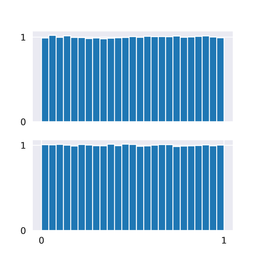
ensuring that the marginal distribution of the second component is uniform and thus the modeling of exact tails. We refer to (9) as a constrained bivariate copula flow.
6 Numerical Results
Due to the positive results of DDSFs [16] and thus the effectiveness of marginal flows we restrict ourselves to the evaluation of copula flows. Specifically, we evaluate the generative capabilities of copula flows on three different tasks, generating the Clayton, Frank and Gumbel copula. Before we report our results we introduce the following metrics and divergences used to compare the distributions.
6.1 Metrics and Divergences
The first performance measure we track is the Jensen-Shannon divergence (JSD) of the targeted copula and the approximation , which we denote by . Furthermore, to assess whether the marginal distributions generated by the copula flow are uniform we approximate via Monte Carlo for and the metric
where . Last, we also compute the maximum of each density estimator
6.2 Benchmarks
The results obtained by training a copula flow on the different theoretical benchmarks can be viewed in Table 1. In order to optimize the copula flow we used a batch size of 3E+03. The training of the copula flow was stopped after a breaking criterion was obtained, which we defined by setting thresholds for each of the metrics in Table 1. The metrics and were evaluated by using a batch size of 5E+05, the NLL with a batch size equal to the training batch size, and the Jensen-Shannon divergence was obtained by evaluating the theoretical and approximated density on a (equidistant) mesh-grid of size .555Due to numerical instabilities of the theoretical copula densities evaluations with nans were discarded.
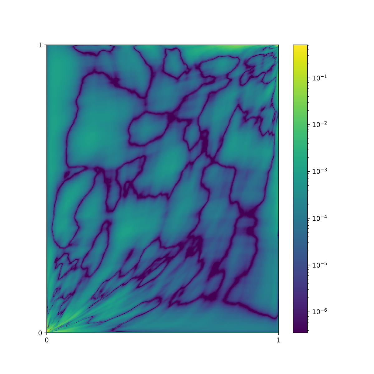
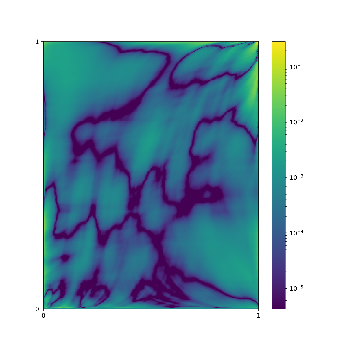
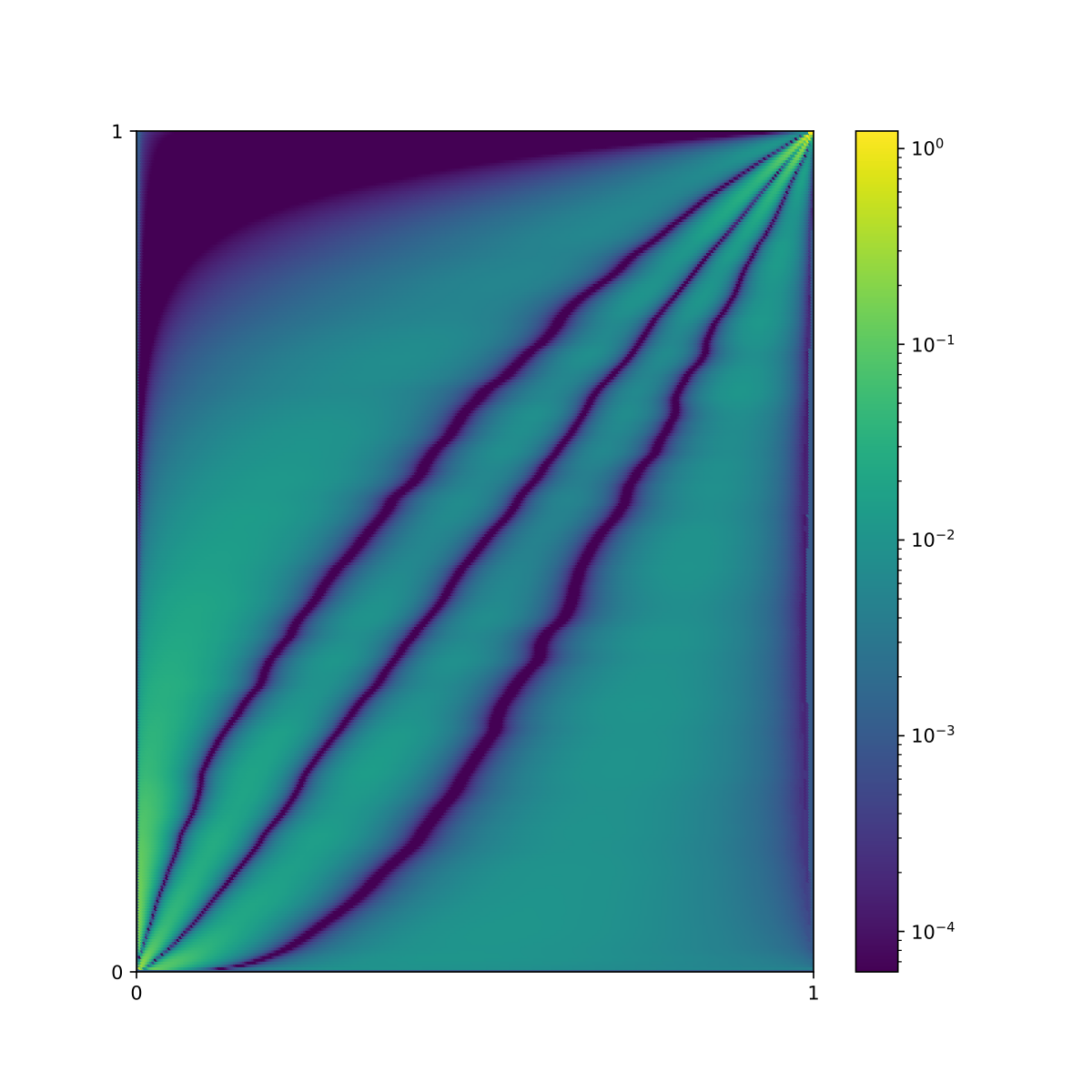
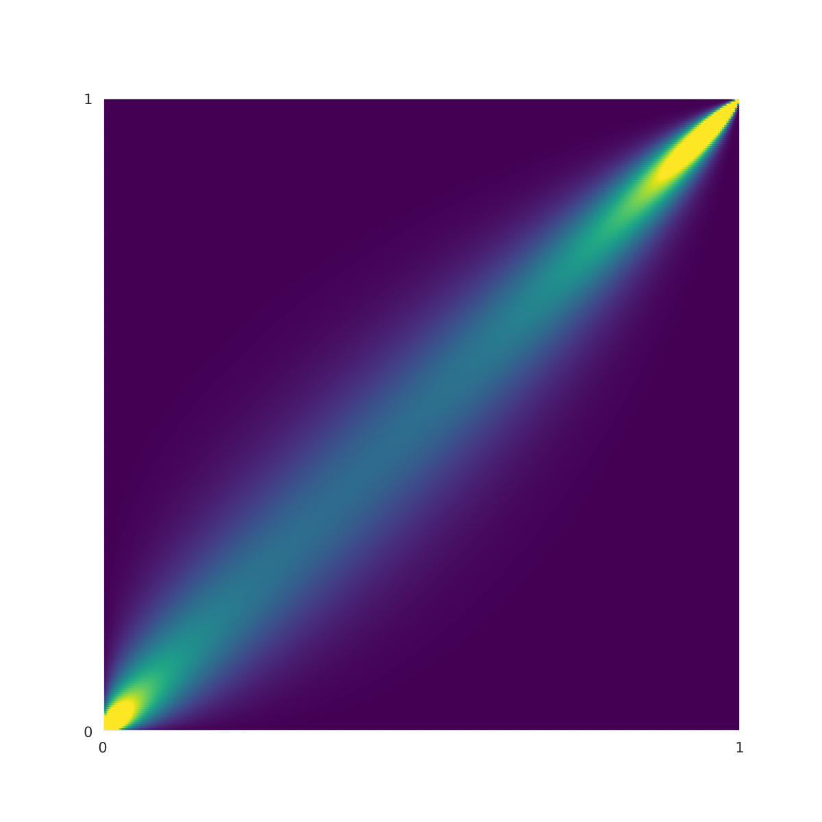
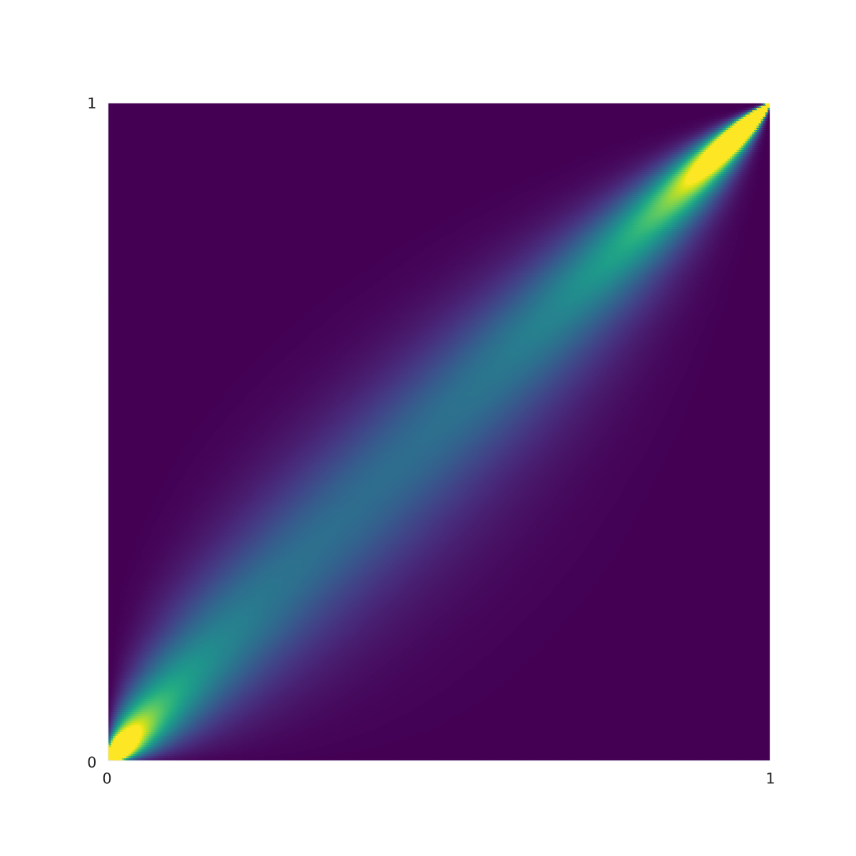
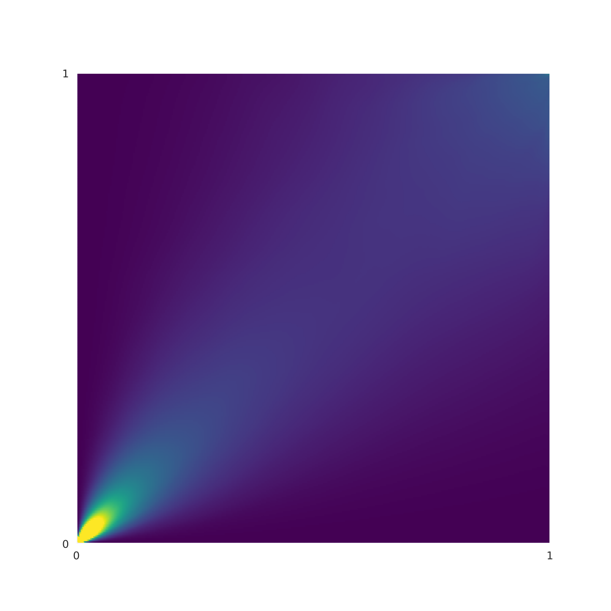
Figure 5 and Figure 5 illustrate the theoretical and approximated density on the Clayton and Frank copula benchmark. Figure 6 in Appendix A depicts the Clayton, Gumbel and Frank copula when evaluating the JSD pointwise on a mesh-grid of size . Lighter colors depict areas that were approximated not as well.



| Copula / Metrics | ||||||
|---|---|---|---|---|---|---|
| \clineB1-72.5 Clayton(2) | 2.40E-04 | 1.17E-04 | 1.27E-04 | 4.04E-02 | 5.06E-02 | -4.41E-01 |
| Frank(5) | 6.89E-04 | 1.64E-04 | 1.71E-04 | 4.98E-02 | 4.68E-02 | -2.56E-01 |
| Gumbel(5)* | 5.96E-03 | 1.18E-04 | 1.01E-04 | 3.44E-02 | 3.63E-02 | -1.22E+00 |
| \clineB1-72.5 |
7 Conclusion
In this paper we demonstrated that generative networks do not favor an exact modeling nor an estimation of the tail asymptotics. Since in various applications an exact modeling of the tail is of major importance we introduced and proposed CM flows. CM flows were explicitly constructed by using a marginal and copula flow which build up on the success of DDSFs and Real NVPs. The numerical results empirically demonstrated that bivariate copulas can be closely approximated by a copula flow and thus support the use of CM flows.
For CM flows to flourish we leave it as future work to correct the marginal distributions induced by a copula flow to be uniform. Once this is achieved, an exact modeling of the marginal distribution will be possible and tails can be modeled in unprecedented ways with deep generative flows.
References
- [1] Kjersti Aas, Claudia Czado, Arnoldo Frigessi and Henrik Bakken “Pair-Copula Constructions of Multiple Dependence” In Insurance: Mathematics and Economics 44, 2009, pp. 182–198
- [2] Martín Arjovsky and Léon Bottou “Towards Principled Methods for Training Generative Adversarial Networks” In CoRR abs/1701.04862, 2017 arXiv:1701.04862
- [3] Bolton Bailey and Matus J Telgarsky “Size-Noise Tradeoffs in Generative Networks” In Advances in Neural Information Processing Systems 31 Curran Associates, Inc., 2018, pp. 6490–6500
- [4] H. Bauer “Wahrscheinlichkeitstheorie”, De-Gruyter-Lehrbuch de Gruyter, 2002 URL: https://books.google.de/books?id=G87VCyJHsb0C
- [5] Tim Bedford and Roger Cooke “Vines - A new graphical model for dependent random variables” In Annals of Statistics 30, 1999
- [6] Andrew Brock, Jeff Donahue and Karen Simonyan “Large Scale GAN Training for High Fidelity Natural Image Synthesis” In CoRR abs/1809.11096, 2018 arXiv: http://arxiv.org/abs/1809.11096
- [7] Laurens De Haan and Ana Ferreira “Extreme value theory: an introduction” Springer Science & Business Media, 2007
- [8] Laurent Dinh, David Krueger and Yoshua Bengio “NICE: Non-linear Independent Components Estimation” In 3rd International Conference on Learning Representations, ICLR 2015, San Diego, CA, USA, May 7-9, 2015, Workshop Track Proceedings, 2015 URL: http://arxiv.org/abs/1410.8516
- [9] Laurent Dinh, Jascha Sohl-Dickstein and Samy Bengio “Density estimation using Real NVP” In CoRR abs/1605.08803, 2016 arXiv: http://arxiv.org/abs/1605.08803
- [10] Gal Elidan “Copula Bayesian Networks” In Advances in Neural Information Processing Systems 23 Curran Associates, Inc., 2010, pp. 559–567 URL: http://papers.nips.cc/paper/3956-copula-bayesian-networks.pdf
- [11] Kolbjørn Engeland, Hege Hisdal and Arnoldo Frigessi “Practical Extreme Value Modelling of Hydrological Floods and Droughts: A Case Study” In Extremes 7, 2004, pp. 5–30
- [12] Ian J. Goodfellow et al. “Maxout Networks” In Proceedings of the 30th International Conference on International Conference on Machine Learning - Volume 28, ICML’13 Atlanta, GA, USA: JMLR.org, 2013, pp. III-1319–III-1327 URL: http://dl.acm.org/citation.cfm?id=3042817.3043084
- [13] Ian Goodfellow et al. “Generative Adversarial Nets” In Advances in Neural Information Processing Systems 27 Curran Associates, Inc., 2014, pp. 2672–2680
- [14] Kaiming He, Xiangyu Zhang, Shaoqing Ren and Jian Sun “Delving Deep into Rectifiers: Surpassing Human-Level Performance on ImageNet Classification” In Proceedings of the 2015 IEEE International Conference on Computer Vision (ICCV), ICCV ’15 Washington, DC, USA: IEEE Computer Society, 2015, pp. 1026–1034
- [15] Kurt Hornik “Approximation capabilities of multilayer feedforward networks” In Neural Networks 4.2, 1991, pp. 251–257 URL: http://www.sciencedirect.com/science/article/pii/089360809190009T
- [16] Chin-Wei Huang, David Krueger, Alexandre Lacoste and Aaron C. Courville “Neural Autoregressive Flows” In CoRR abs/1804.00779, 2018 arXiv: http://arxiv.org/abs/1804.00779
- [17] Ralf Korn, Elke Korn and Gerald Kroisandt “Monte Carlo Methods and Models in Finance and Insurance”, 2010
- [18] Nicole Krämer and Ulf Schepsmeier “Introduction to Vine Copulas” In Introduction to Vine Copulas (NIPS 2008 Workshop), Granada, Spain, 2011
- [19] Yann LeCun, Léon Bottou, Genevieve B. Orr and Klaus-Robert Müller “Efficient BackProp” In Neural Networks: Tricks of the Trade, This Book is an Outgrowth of a 1996 NIPS Workshop London, UK, UK: Springer-Verlag, 1998, pp. 9–50 URL: http://dl.acm.org/citation.cfm?id=645754.668382
- [20] Lars M. Mescheder “On the convergence properties of GAN training” In CoRR abs/1801.04406, 2018 arXiv: http://arxiv.org/abs/1801.04406
- [21] Vinod Nair and Geoffrey E. Hinton “Rectified Linear Units Improve Restricted Boltzmann Machines” In Proceedings of the 27th International Conference on International Conference on Machine Learning, ICML’10 Haifa, Israel: Omnipress, 2010, pp. 807–814 URL: http://dl.acm.org/citation.cfm?id=3104322.3104425
- [22] William Reed and Murray Jorgensen “The Double Pareto-Lognormal Distribution—A New Parametric Model for Size Distributions” In Communications in Statistics. Theory and Methods 8, 2004
- [23] Danilo Jimenez Rezende and Shakir Mohamed “Variational Inference with Normalizing Flows” In Proceedings of the 32Nd International Conference on International Conference on Machine Learning - Volume 37, ICML’15 Lille, France: JMLR.org, 2015, pp. 1530–1538 URL: http://dl.acm.org/citation.cfm?id=3045118.3045281
- [24] Hilary L. Seal “Survival Probabilities Based on Pareto Claim Distributions” In ASTIN Bulletin 11.1 Cambridge University Press, 1980, pp. 61–71
Appendix A Proofs
Proof of subsection 4.2.
∎
Proof of subsection 4.2.
Since is not affinely lighter tailed than it can be shown that for any there exists an affine function such that is not affinely lighter tailed than , where is the function from Theorem 1, implying
Then by Theorem 1 we obtain that for any
which implies that the set of optimal generative networks is empty. ∎
Appendix B Basic Definitions
Definition \thedefinition (Activation Function).
A function that is Lipschitz continuous, monotonic and satisfies is called activation function.
Remark \theremark.
Appendix B comprises a large class of functions found in literature [12, 14, 21, 19].
Definition \thedefinition (Deep Dense Sigmoidal Flow).
Let such that . Moreover, for let and two non-negative matrices for which their row-wise sum is equal to . Furthermore, let define an invertible CDF. A function
where is defined recursively for through
| (10) |
is called a deep dense sigmoidal flow.
Appendix C Additional Numerical Results
