capbtabboxtable[][\FBwidth]
Improving Detection of Credit Card Fraudulent Transactions using Generative Adversarial Networks
Abstract
In this study, we employ Generative Adversarial Networks as an oversampling method to generate artificial data to assist on the classification of credit card fraudulent transactions. GANs is a generative model that based on the idea of game theory, in which a generator G and a discriminator D are trying to outsmart each other. The objective of the generator is to confuse the discriminator. The objective of the discriminator is to distinguish the instances coming from the generator and the instances coming from the original dataset. By training GANs on a set of credit card fraudulent transactions, we are able to improve the discriminatory power of classifiers. The experiment results show that the Wasserstein-GAN is more stable in training and produce more realistic fraudulent transactions than the other GANs. On the other hand, the conditional version of GANs in which labels are set by k-means clustering does not necessarily improve the non-conditional versions of GANs.
keywords:
generative adversarial networks; imbalanced learning; creditcard, fraudulent transactions1 Introduction
Credit cards are used as a crucial payment method in modern society, and more fraudulent transactions are increasingly produced in the overwhelming of credit card usages. Fraudulent transactions affect not only the banks and merchants but also the end users because even if they get reimbursement, they could eventually pay more for a higher fee of credit card services.
In this study, we employ Generative Adversarial Networks (GANs, Goodfellow et al. (2014)) as an oversampling method to generate artificial data to assist with the classification of credit card fraudulent transactions. GANs is a generative model based on the idea of game theory, in which a generator G and a discriminator D are trying to outsmart each other. The objective of the generator is to confuse the discriminator. The objective of the discriminator is to distinguish the instances coming from the generator and the instances coming from the original dataset. By training GANs on a set of fraudulent transactions and then generating fake fraud transactions to balance the dataset, we compare different oversampling methods on creditcard fraudulent detection.
2 Literature Review
On the distribution of classes, credit granting process and fraud detection are of the sources that produce the highest degree of imbalanced classes. Imbalance dataset (IDS) has almost observations which belong to majority class - good applications and the other belong to a small number of minority class - bad applications. To handle imbalanced dataset, random oversampling the minority class and undersampling the majority class are two common sampling methods. However, oversampling will easily be trapped into overfitting where as undersampling may discard useful data that leads to information loss He and Garcia (2009). As an improvement to random up sampling, Synthetic Minority Over-sampling Technique (SMOTE) Chawla et al. (2002) synthesizes artificial data in the minority class instead of replication. Random Over-Sampling Examples (ROSE) Menardi and Torelli (2014) generalizes the standard technique of oversampling with replacement the rare examples by allowing the generation of some clones of the observed data, without producing ties.
The most recent work of the application of GANs on creating artificial samples to balance the class in classification problems is Douzas and Bacao (2018), cGAN performance was evaluated on 71 datasets with different imbalance ratios, number of features and subclustering structures and compared to multiple oversampling methods, using Logistic Regression, Support Vector Machine, Nearest Neighbors, Decision Trees and Gradient Boosting Machine as classifiers. The results show that cGAN performs better compared to the other methods for a variety of classifiers, evaluation metrics and datasets with complex structure. The explanation for this improvement in performance relates to the ability of cGAN to recover the training data distribution, if given enough capacity and training time.
3 Methodology
In this section, we provide oversampling background followed by a summary of the GAN, cGAN, WGAN, and WCGAN frameworks following closely the notation in Goodfellow et al. (2014), Gauthier (2014), Arjovsky et al. (2017) and Gulrajani et al. (2017).
3.0.1 Oversampling
Popular oversampling methods including Random Oversampling (ROS), SMOTE, and ADASYN Haixiang et al. (2017) will be used. ROS balances data by randomly duplicating the minority samples. SMOTE selects K nearest neighbors, connects them and forms the synthetic samples. By adaptively changing the weights of the different minority samples to compensate for the skewed distributions, ADASYN uses a density distribution, as a criterion to automatically decide the number of synthetic samples that must be generated for each minority sample.
3.0.2 GAN and CGAN
The generative model , defined as where is the noise space and is the data space, aims to capture the real data distribution. The discriminator, defined as , estimates the probability that a sample came from the real data distribution rather than the data space generated by . These two models, which could be both multilayer perceptron, compete in a two-player minimax game with value function:
| (3.1) |
The value and are sampled from the real data distribution and noise distribution respectively. The GAN training procedure could be step(s) for and one optimizing step for by means of stochastic gradient descent (SGD).
Instead of minimizing the probability of generated samples being detected as fake, to prevent vanishing gradient, the optimization process of could focus on generating as real as possible the noise sample to confuse (non-saturating GANs).
| (3.2) |
The cGAN extends the GAN framework by adding an additional space from the real data as follow:
and
And the 3.0.2 changes as:
where:
. and
.
The training process of cGAN is almost similar with GAN. By feeding a minibatch of training examples and noise random samples , the logistic cost function for the gradient update of and is as follow:
| (3.3) |
| (3.4) |
3.1 WGAN and WCGAN
Arovsky et. al., 2017, uses Earth Mover (EM) distance to learn the probability distribution of real data. They propose Wasserstein-GAN (WGAN) to minimize EM distance and the WGAN shows that it could cure the training problem of GANs which requires carefully design of network structures and the balance in training of and . Specifically, the loss function on training WGAN is:
| (3.5) |
| (3.6) |
where is a 1-Lipschitz continuous function, parameterized by , that the “Discriminator” model need to learn. we could find the details mathematical claims in the original paper of authors.
3.2 Experimental Setup
We use credit card transactions data from Pozzolo et al. (2015), which includes a subset of online transactions and consists of 31 coded features. We have 492 frauds out of 284,807 transactions. The dataset is highly imbalanced with the positive class (frauds) accounts for just 0.172%. The random search is employed for tuning the hyperparameters of GANs frameworks, and the results are reported under 10-fold nested cross-validation (cv).
The data consists of 31 features: “time”,“amount”, “class” and 28 additional, anonymized features. The class feature is the label indicating whether a transaction is fraudulent or not, with 0 and 1 indicating normal and fraud transaction, respectively. All of the data is numeric and continuous (except the label). The data set has no missing values.
For a fast implementation of classification algorithm, we use XGBoost (Chen and Guestrin, 2016) with max depth equals 4 and area under the curve as an evaluation matric.
In this study, we employ GAN as an oversampling method to increase number of the minority class by using the trained, converged generator to create artificial fraud samples. All four GANs models are trained on the full fraud samples, the stopping criteria is defined by manually investigating the loss of both generator and discriminator. We use 10-fold cross validation to examine the quality of generated fraudulent transactions. Let and be the number of normal and fraudulent transactions of fold , respectively. The experiment procedure could be summarized as follows:
for in number of folds do:
1. separate data to training set: and test set: :
2. for number of training iterations do:
-
•
Generate artificial samples .
-
•
Train using both real samples and
-
•
Train combined model .
-
•
Log XGB predictive performance on classifying and real samples.
-
•
Find the iteration at which XGB performance is lowest.
3. Find the iteration at which XGB performance is lowest.
4. Generate artificial data such that .
5. Train and test XGB on the augmented training data and , respectively.
3.2.1 Performance Measurements
To compare seven sampling methods, we train one classifier, Logistic Regression (LR), on balanced data and examine its performance on a separate test set with Area under the ROC curve (AUC), Area under the PR curve (AUPRC), Recall, Precision, and F1-Score. We pay attention to the categorical prediction ability since transaction stagnation causes by misclassifying the normal transactions also threatens the customer relationships of the merchants or financial institutions.
4 Results
All four GANs models are trained on 80% fraud samples, the stopping criterion is defined by investigating the loss of both generator and discriminator, at which we use to generate artificial fraud data.
Table 1 show the hyperparameters of four GANs frameworks found by random search, it should be noted that we only search for learning rate, drop-out rate, and the number of notes in the 3-layer perceptrons. The network architectures are fixed with three layers and trained with mini-batch of 64 samples, Adam optimizer, and Leaky-Relu activation function ().
| Learning | Drop-Out | #Nodes | |
|---|---|---|---|
| Rate | Rate | ||
| GAN | 0.029 | 0.5 | 85 |
| CGAN | 0.036 | 0.4 | 46 |
| WGAN | 0.011 | 0.5 | 63 |
| WCGAN | 0.022 | 0.22 | 5 |
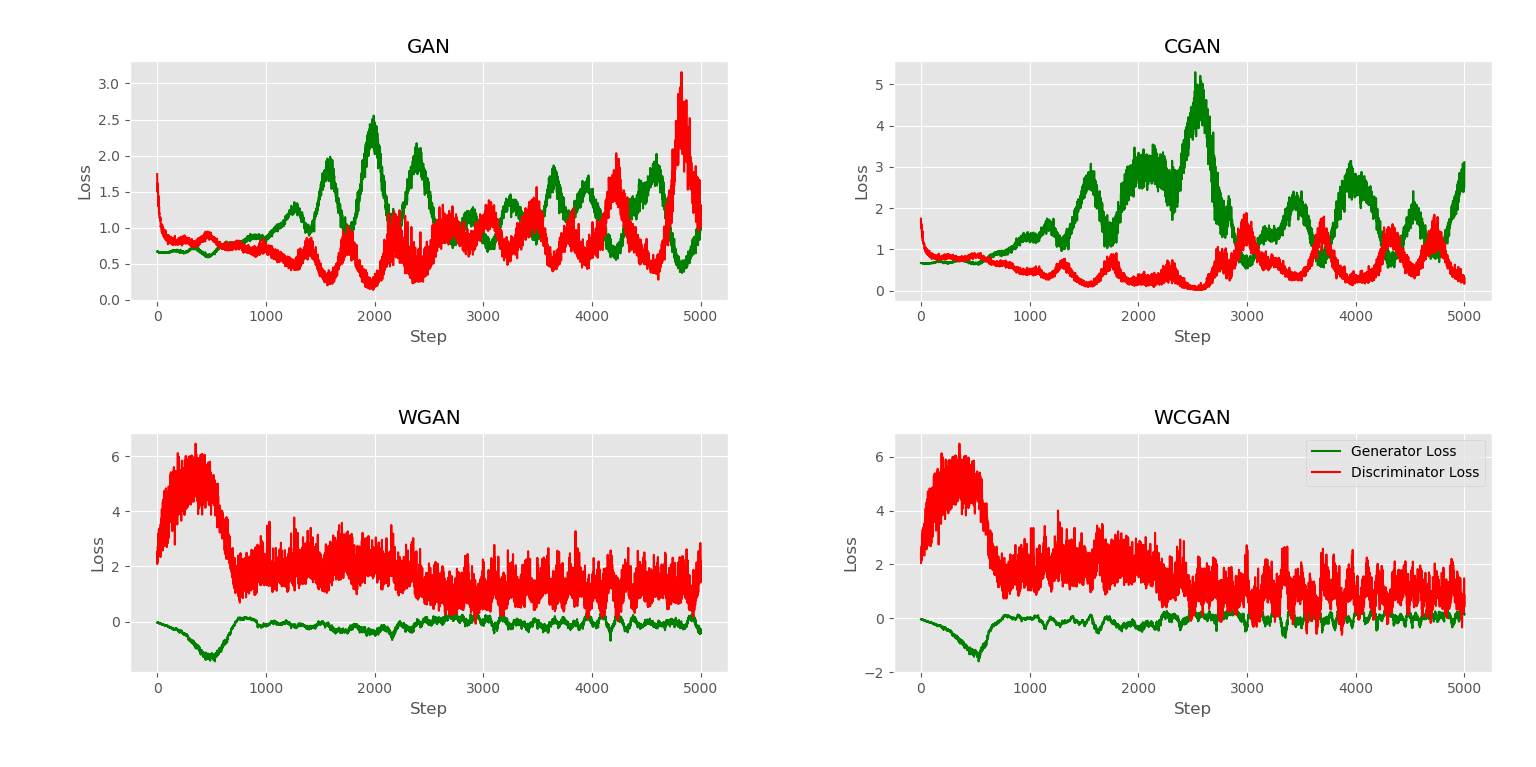
Figure 1 presents the loss of both D and G during the first epoch. While we observe the losses of WGAN variants are stable after 1000 iterations, vanilla GANs (GAN and CGAN) do not actually convert. Hence, we further check for the quality of generated data using Extreme Gradient Boosting Machine (XGB). The step at which we stop training GANs is the step that leads to the lowest accuracy of XGB on discriminating the real and the fake, generated fraud transactions.

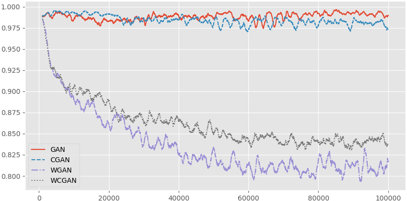
From our tests, it appears that our best architecture is the WGAN/WCGAN at the training iteration near 3000 or 5000 as shown in Figure 2,

at the latter step, WGAN/WCGAN achieved an xgboost accuracy of 86% on detecting fraudulent and generated data (ideally, accuracy would be 50%). We use all four architectures to generate new fraud data.
And to check how efficient the generated data help with detecting fraud credit card transaction, we use up to 80% of the non-fraudulent data and fraud data. Different amounts of real or generated fraud data are added to this training set, up to 80% of the fraud data. For the test set, we use the other 20% of the non-fraud cases and fraud cases. By adding generated data from both an untrained GANs and the best trained GANs to test if the generated data is any better than random noise.


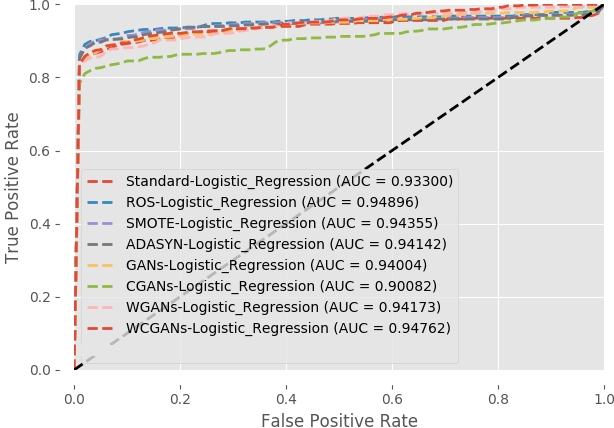
Figure 4 presents all ROC curves of seven balancing methods and compares them with none sampling setting. As credit card transactions are dominated by the normal transactions, we would focus on the far left-hand side of the ROC curves where ROS and ADASYN are better than the rest.

The cv performance of LR classifier are shown in Table 2 with five metrics under seven balancing methods. Bold values represent the best. The first row is LR prediction with no sampling and the Rank in the final column is the average rank across five metrics.
| AUC | AUPRC | Recall | Precison | F1-Score | Rank | |
|---|---|---|---|---|---|---|
| None | 0.933 | 0.745 | 0.581 | 0.908 | 0.680 | 3.8 |
| ROS | 0.949 | 0.750 | 0.882 | 0.067 | 0.123 | 3.2 |
| SMOTE | 0.944 | 0.750 | 0.876 | 0.062 | 0.113 | 4.4 |
| ADASYN | 0.941 | 0.730 | 0.901 | 0.018 | 0.035 | 5.2 |
| GAN | 0.940 | 0.637 | 0.502 | 0.777 | 0.501 | 5.6 |
| CGAN | 0.901 | 0.631 | 0.564 | 0.643 | 0.444 | 6.4 |
| WGAN | 0.942 | 0.723 | 0.803 | 0.500 | 0.583 | 4.2 |
| WCGAN | 0.948 | 0.717 | 0.642 | 0.852 | 0.710 | 3.2 |
In AUC, ROS comes first with WCGAN follows closely. Whereas in AUPRC, vanilla balancing methods including the none sampling setting are better than all four GANs frameworks. However, in term of quality and quantity of fraudulent detection, GANs frameworks produce more balancing values in Recall and Precision, which result in better F1-Score.
5 Conclusions
-
•
Potential application of simple GANs frameworks in enhancing the fraudulent detection in credit card transacions.
-
•
GANs are able to learn distributions in situations where the divergence minimization might predict they would fail Fedus et al. (2017).
-
•
Wasserstein-GAN is more stable in training and produce more realistic fraudulent transactions than the other GANs.
-
•
The conditional version of GANs in which labels are set by k-means clustering does not necessarily improve the non-conditional versions.
Acknowledgements
This research is supported by JAIST Off-Campus Research Grant and Doctoral Research Fellow Grant No. 238003. We thank Professor Gary Bolton for his comments when the earlier version of this paper was presented in the Game Theory Conference, Edinburgh, UK, March 2019. All errors retain our own.
References
- Arjovsky et al. (2017) Arjovsky, M., Chintala, S., and Bottou, L. (2017). Wasserstein GAN. arXiv:1701.07875 [cs, stat]. arXiv: 1701.07875.
- Chawla et al. (2002) Chawla, N. V., Bowyer, K. W., Hall, L. O., and Kegelmeyer, W. P. (2002). SMOTE: synthetic minority over-sampling technique. Journal of artificial intelligence research, 16:321–357.
- Chen and Guestrin (2016) Chen, T. and Guestrin, C. (2016). XGBoost: A Scalable Tree Boosting System. In Proceedings of the 22nd ACM SIGKDD International Conference on Knowledge Discovery and Data Mining - KDD ’16, pages 785–794, San Francisco, California, USA. ACM Press.
- Douzas and Bacao (2018) Douzas, G. and Bacao, F. (2018). Effective data generation for imbalanced learning using conditional generative adversarial networks. Expert Systems with Applications, 91:464–471.
- Fedus et al. (2017) Fedus, W., Rosca, M., Lakshminarayanan, B., Dai, A. M., Mohamed, S., and Goodfellow, I. (2017). Many Paths to Equilibrium: GANs Do Not Need to Decrease a Divergence At Every Step. arXiv:1710.08446 [cs, stat]. arXiv: 1710.08446.
- Gauthier (2014) Gauthier, J. (2014). Conditional generative adversarial nets for convolutional face generation. Class Project for Stanford CS231N: Convolutional Neural Networks for Visual Recognition, Winter semester.
- Goodfellow et al. (2014) Goodfellow, I., Pouget-Abadie, J., Mirza, M., Xu, B., Warde-Farley, D., Ozair, S., Courville, A., and Bengio, Y. (2014). Generative Adversarial Nets. In Ghahramani, Z., Welling, M., Cortes, C., Lawrence, N. D., and Weinberger, K. Q., editors, Advances in Neural Information Processing Systems 27, pages 2672–2680. Curran Associates, Inc.
- Gulrajani et al. (2017) Gulrajani, I., Ahmed, F., Arjovsky, M., Dumoulin, V., and Courville, A. (2017). Improved Training of Wasserstein GANs. arXiv:1704.00028 [cs, stat]. arXiv: 1704.00028.
- Haixiang et al. (2017) Haixiang, G., Yijing, L., Shang, J., Mingyun, G., Yuanyue, H., and Bing, G. (2017). Learning from class-imbalanced data: Review of methods and applications. Expert Systems with Applications, 73:220–239.
- He and Garcia (2009) He, H. and Garcia, E. A. (2009). Learning from Imbalanced Data. IEEE Transactions on Knowledge and Data Engineering, 21(9):1263–1284.
- Menardi and Torelli (2014) Menardi, G. and Torelli, N. (2014). Training and assessing classification rules with imbalanced data. Data Mining and Knowledge Discovery, 28(1):92–122.
- Pozzolo et al. (2015) Pozzolo, A. D., Caelen, O., Johnson, R. A., and Bontempi, G. (2015). Calibrating Probability with Undersampling for Unbalanced Classification. In 2015 IEEE Symposium Series on Computational Intelligence, pages 159–166.