Contextuality and noncontextuality measures and generalized Bell inequalities for cyclic systems

Abstract

Cyclic systems of dichotomous random variables have played a prominent role in contextuality research, describing such experimental paradigms as the Klyachko-Can-Binicioğlu-Shumovsky, Einstein-Podolsky-Rosen-Bell, and Leggett-Garg ones in physics, as well as conjoint binary choices in human decision making. Here, we understand contextuality within the framework of the Contextuality-by-Default (CbD) theory, based on the notion of probabilistic couplings satisfying certain constraints. CbD allows us to drop the commonly made assumption that systems of random variables are consistently connected (i.e., it allows for all possible forms of “disturbance” or “signaling” in them). Consistently connected systems constitute a special case in which CbD essentially reduces to the conventional understanding of contextuality. We present a theoretical analysis of the degree of contextuality in cyclic systems (if they are contextual) and the degree of noncontextuality in them (if they are not). By contrast, all previously proposed measures of contextuality are confined to consistently connected systems, and most of them cannot be extended to measures of noncontextuality. Our measures of (non)contextuality are defined by the $L_{1}$-distance between a point representing a cyclic system and the surface of the polytope representing all possible noncontextual cyclic systems with the same single-variable marginals. We completely characterize this polytope, as well as the polytope of all possible probabilistic couplings for cyclic systems with given single-variable marginals. We establish that, in relation to the maximally tight Bell-type CbD inequality for (generally, inconsistently connected) cyclic systems, the measure of contextuality is proportional to the absolute value of the difference between its two sides. For noncontextual cyclic systems, the measure of noncontextuality is shown to be proportional to the smaller of the same difference and the $L_{1}$-distance to the surface of the box circumscribing the noncontextuality polytope. These simple relations, however, do not generally hold beyond the class of cyclic systems, and noncontextuality of a system does not follow from noncontextuality of its cyclic subsystems.

I Introduction

A cyclic system of rank $n=2,3,\ldots$, is a system

$$\mathcal{R}=\left\{\left\{R_{i}^{i},R_{i\oplus 1}^{i}\right\}:i=1,\ldots,n\right\},$$ (1)

where $i\oplus 1=i+1$ for $i<n$, and $n\oplus 1=1$; $R_{j}^{i}$ denotes a Bernoulli ($0/1$) random variable measuring content $q_{j}$ in context $c_{i}$ ($j=i,i\oplus 1$). A content is any property that can be present or absent (e.g., spin of a half-spin particle in a given direction), a context here is defined by which two contents are measured together (simultaneously or in a specific order). A cyclic system of rank $n$ has $n$ contexts containing two jointly distributed random variables each, $\left\{R_{i}^{i},R_{i\oplus 1}^{i}\right\}$. Each of such pairs is referred to as a bunch (of random variables). The system also has $n$ connections $\left\{R_{i}^{i\ominus 1},R_{i}^{i}\right\}$ (where $i\ominus 1=i-1$ for $i>1$, and $1\ominus 1=n$), each of which contains two stochastically unrelated (i.e., possessing no joint distribution) random variables measuring the same content in two different contexts.

Cyclic systems have played a prominent role in contextuality studies (Araujoetal2013, ; KujDzhLar2015, ). The matrices below represent cyclic systems of rank 5 (describing, e.g., the Klyachko-Can-Binicioğlu-Shumovsky experiment (KCBS2008, ; Lapkiewicz2015, )), rank 4 (describing, e.g., Bell’s “Alice-Bob” experiments (Bell1964, ; Bell1966, ; Fine1982, ; CHSH1969, )), rank 3 (describing, e.g., the Leggett-Garg experiments (LeggGarg1985, ; Bacciagaluppi2015, ; KoflerBrukner2013, ; SuppesZanotti1981, )), and rank 2 (of primary interest outside quantum physics, e.g., describing the question-order experiment in human decision making (DzhZhaKuj2016, ; Wang, )).

$$\begin{array}[]{cc}\begin{array}[]{|c|c|c|c|c||c|}\hline\cr R_{1}^{1}&R_{2}^{1}&&&&c^{1}\\ \hline\cr&R_{2}^{2}&R_{3}^{2}&&&c^{2}\\ \hline\cr&&R_{3}^{3}&R_{4}^{3}&&c^{3}\\ \hline\cr&&&R_{4}^{4}&R_{5}^{4}&c^{4}\\ \hline\cr R_{1}^{5}&&&&R_{5}^{5}&c^{5}\\ \hline\cr\hline\cr q_{1}&q_{2}&q_{3}&q_{4}&q_{5}&\mathcal{R}_{5}\\ \hline\cr\end{array}&\begin{array}[]{|c|c|c|c||c|}\hline\cr R_{1}^{1}&R_{2}^{1}&&&c^{1}\\ \hline\cr&R_{2}^{2}&R_{3}^{2}&&c^{2}\\ \hline\cr&&R_{3}^{3}&R_{4}^{3}&c^{3}\\ \hline\cr R_{1}^{4}&&&R_{4}^{4}&c^{4}\\ \hline\cr\hline\cr q_{1}&q_{2}&q_{3}&q_{4}&\mathcal{R}_{4}\\ \hline\cr\end{array}\\ \\ \begin{array}[]{|c|c|c||c|}\hline\cr R_{1}^{1}&R_{2}^{1}&&c^{1}\\ \hline\cr&R_{2}^{2}&R_{3}^{2}&c^{2}\\ \hline\cr R_{1}^{3}&&R_{3}^{3}&c^{3}\\ \hline\cr\hline\cr q_{1}&q_{2}&q_{3}&\mathcal{R}_{3}\\ \hline\cr\end{array}&\begin{array}[]{|c|c||c|}\hline\cr R_{1}^{1}&R_{2}^{1}&c^{1}\\ \hline\cr R_{1}^{2}&R_{2}^{2}&c^{2}\\ \hline\cr\hline\cr q_{1}&q_{2}&\mathcal{R}_{2}\\ \hline\cr\end{array}\end{array}$$ (2)

A cyclic system is consistently connected (satisfies the “no-disturbance” or “no-signaling” condition) if $R_{i}^{i}$ and $R_{i}^{i\ominus 1}$ are identically distributed for $i=1,\ldots,n$. This assumption is commonly made in quantum physical applications. The present paper, however, is based on the Contextuality-by-Default (CbD) theory (DzhCerKuj2017, ; KujDzhMeasures, ; DzhKujFoundations2017, ), which is not predicated on this assumption, that is, the systems of random variables we consider are generally inconsistently connected. Cyclic systems have been intensively analyzed within the framework of CbD (Bacciagaluppi2015, ; DzhKujLar2015, ; DzhZhaKuj2016, ; KujDzhLar2015, ; KujDzhProof2016, ). In this paper they are studied in relation to the measures of contextuality and noncontextuality considered in Ref. (KujDzhMeasures, ).

The familiarity of the reader with CbD (e.g., Refs. (DzhCerKuj2017, ; KujDzhMeasures, )) for understanding this paper is not necessary, even if desirable. We recapitulate here all relevant definitions and results, although they are presented in the form specialized to cyclic systems rather than in complete generality, so the broader motivation behind the constructs may not always be apparent. In particular, we take it for granted in this paper that it is important not to be constrained by the confines of consistent connectedness (KujDzhLar2015, ; DzhKujLar2015, ). The simplest reason for this is that if a consistently connected system is contextual or noncontextual by one’s definition, then it is reasonable to require from this definition that the system’s contextuality status should not change under sufficiently small perturbations rendering it inconsistently connected. Another reason is that inconsistent connectedness is ubiquitous. Thus, in accordance with the quantum-mechanical laws, consistent connectedness does not generally hold for sequential measurements, e.g., for the Leggett-Garg system (KoflerBrukner2013, ; Bacciagaluppi2015, ). In other experimental paradigms it is often violated due to unavoidable or inadvertent design biases (Lapkiewicz2015, ). In all such cases, use of CbD to analyze data has proved to be useful (Malinowskietal., ; Ariasetal.2015, ; Crespietal.2017, ; Fluhmannetal2018, ; Zhanetal.2017, ; KujDzhLar2015, ; Bacciagaluppi2015, ). At the same time, all contextuality measures proposed outside CbD are confined to consistent connectedness (Grudkaetal2014, ; Kleinmanetal2011, ; AbramBarbMans2017, ; Brunneretal2014, ; AmaralCunhaCabello2015, ).

We also take for granted in this paper that it is desirable to seek principled and unified ways of measuring both contextuality and noncontextuality (KujDzhMeasures, ). Degree of contextuality has been related to such concepts as quantum advantage in computation and communication complexity (Bermejoetal2017, ; Howardetal.2014, ; Brukneretal.2004, ), and generally is viewed as a measure of nonclassicality of a system. Moreover, it is intrinsically interesting to compare different contextual systems in terms of which of them can be more easily rendered noncontextual by perturbing its random variables (see Ref. (Brunneretal2014, ) for an overview). Intrinsic interest in measures of noncontextuality can be justified similarly. It is too uninformative to simply view noncontextual systems as having zero contextuality: some of them would be easier than others to render contextual by perturbing their random variables. Remarkably, there seem to be no measures of noncontextuality proposed in the literature prior to Ref. (KujDzhMeasures, ), and most of the proposed measures of contextuality (e.g., the Contextual Fraction measure proposed in Ref. (AbramBarbMans2017, ) and generalized to inconsistently connected systems in Ref. (KujDzhMeasures, )) do not naturally extend to measures of noncontextuality. By “natural extension” we mean the extension to noncontextual systems using the same principles as in constructing a contextuality measure being extended.

Note that the term “degree of noncontextuality” in this paper always applies to noncontextual systems only, in the same way as “degree of contextuality” only applies to contextual systems. This is useful to mention because “degree of noncontextuality” has been used in the literature in a different meaning: as a measure complementary to the degree of contextuality in contextual systems. Thus, the Noncontextual Fraction measure in Ref. (AbramBarbMans2017, ) is unity minus Contextual Fraction measure. Both are defined for contextual systems, while noncontextual ones all have Noncontextual Fraction equal to unity.

Of the several measures of contextuality considered in Ref. (KujDzhMeasures, ) we focus here on two, labeled $\textnormal{CNT}_{1}$ and $\textnormal{CNT}_{2}$. The former is the oldest measure introduced within the framework of CbD (DzhKujLar2015, ; KujDzhLar2015, ; KujDzhProof2016, ), whereas $\textnormal{CNT}_{2}$ is the newest one, discussed in Ref. (KujDzhMeasures, ). A detailed description of these measures will have to wait until we have introduced the necessary definitions and results. In a nutshell, however, a cyclic system (with the distribution of each of the random variables $R_{j}^{i}$ being fixed) is represented in CbD by two vectors of product expectations, $\mathbf{p_{b}}$ and $\mathbf{p_{c}}$, conventionally referred to as vectors of “correlations.” (We will only use this term, strictly speaking, incorrect, in this informal introduction, due to its familiarity in the contextuality literature.) The subscripts $\mathbf{b}$ and $\mathbf{c}$ stand for the just-defined CbD terms “bunch” and “connection.” The vector $\mathbf{p_{b}}$ encodes the correlations within the bunches $\left\{R_{i}^{i},R_{i\oplus 1}^{i}\right\}$, $i=1,\ldots,n$. The vector $\mathbf{p_{c}}$ encodes the correlations imposed on the within-connection pairs $\left\{R_{i}^{i\ominus 1},R_{i}^{i}\right\}$, $i=1,\ldots,n$, defining thereby so-called couplings of the connections (recall that the connections themselves do not possess joint distributions). A cyclic system whose (non)contextuality we measure is represented by vectors $\mathbf{p_{b}^{*}},\mathbf{p_{c}^{*}}$, where $\mathbf{p_{b}^{*}}$ consists of the observed bunch correlations, and $\mathbf{p_{c}^{*}}$ consists of the correlations computed for the connections in a special way (the maximal couplings of the connections). In the case of $\textnormal{CNT}_{1}$, the $L_{1}$-distance is measured between $\mathbf{\mathbf{p_{c}^{*}}}$ and the feasibility polytope $\mathbb{P}_{\mathbf{c}}$ comprising all possible $\mathbf{p_{c}}$-vectors compatible with $\mathbf{p_{b}^{*}}$. In the case of $\textnormal{CNT}_{2}$, $L_{1}$-distance is computed between $\mathbf{p_{b}^{*}}$ and the noncontextuality polytope $\mathbb{P}_{\mathbf{b}}$ comprising all $\mathbf{p_{b}}$-vectors compatible with $\mathbf{p_{c}^{*}}$. The two measures therefore are, in a well-defined sense, mirror images of each other.

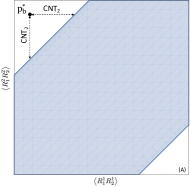
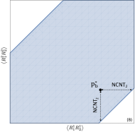
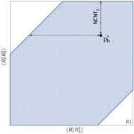
Figure 1: The relationship between a noncontextuality polytope $\mathbb{P}_{\mathbf{b}}$ (light-colored hexagon), the circumscribing box $\mathbb{R}_{\mathbf{b}}$ (rectangle), and a point $\mathbf{p_{b}^{*}}$ representing a system (small circle). The illustration uses cyclic systems of rank 2, shown as $\mathcal{R}_{2}$ in (2). The point $\mathbf{p_{b}^{*}}$ in (A) represents a contextual system, and its $L_{1}$-distance to the polytope is $\textnormal{CNT}_{2}$; it can be measured along any of the (here, two) coordinates. The point $\mathbf{p_{b}^{*}}$ in (B) represents a noncontextual system, and since its $L_{1}$-distance to an internal face of the polytope (here, edge of the hexagon) is smaller than that to the surface of $\mathbb{R}_{\mathbf{b}}$, this distance is $\textnormal{NCNT}_{2}$, and it can be measured along any single coordinate. The point $\mathbf{p_{b}^{*}}$ in (C) represents a noncontextual system which is $L_{1}$-closer to the surface of $\mathbb{R}_{\mathbf{b}}$, and this (also single-coordinate) distance from the surface is $\textnormal{NCNT}_{2}$.

In this paper, we provide a complete characterization of the noncontextuality polytope, and show that the $L_{1}$-distance between this polytope and the observed vector $\mathbf{p_{b}^{*}}$ is a single-coordinate distance, i.e. it can be computed along a single coordinate of $\mathbf{p_{b}}$. Moreover, when $\mathbf{p_{b}^{*}}$ is outside this polytope, this distance is the same along all coordinates of $\mathbf{p_{b}}$ (see Fig. 1A), and it is proportional to the amount of violation of the generalized Bell criterion derived in Ref. (KujDzhProof2016, ) for noncontextuality of (generally inconsistently connected) cyclic systems.(footnote2, ) In other words, if we schematically present the Bell criterion as stating that a system is noncontextual if and only if some expression $E$ does not exceed a constant $k$, then $\textnormal{CNT}_{2}$ is proportional to $E-k$ when this value is positive. Since precisely the same is true for $\textnormal{CNT}_{1}$ (KujDzhProof2016, ), with the same proportionality coefficient, we have

$$\textnormal{CNT}_{2}=\textnormal{CNT}_{1}.$$ (3)

To understand why this is the case, we characterize the polytope $\mathbb{P}$ of all possible vectors $\left(\mathbf{p_{b}},\mathbf{p_{c}}\right)$, and show that its $L_{1}$-distance from the vector $\left(\mathbf{p_{b}^{*}},\mathbf{p_{c}^{*}}\right)$ representing the observed contextual cyclic system has the same properties as above: it is a single-coordinate distance, the same along any of the coordinates of $\left(\mathbf{p_{b}},\mathbf{p_{c}}\right)$. The equality of the two measures follows from this immediately.

Despite the fact that $\textnormal{CNT}_{1}$ and $\textnormal{CNT}_{2}$ are “mirror images” of each other, only one of them, $\textnormal{CNT}_{2}$, was shown in Ref. (KujDzhMeasures, ) to be naturally extendable to a measure of the degree of noncontextuality in noncontextual systems, $\textnormal{NCNT}_{2}$. Geometrically, this measure is the $L_{1}$-distance between a point $\mathbf{p_{b}^{*}}$ inside the noncontextuality polytope $\mathbb{P}_{\mathbf{b}}$ and the polytope’s surface. It is, too, a single-coordinate distance (as is the case for any internal point of any convex region (Tuenter2006, )), but its properties are somewhat more complicated due to the structure of $\mathbb{P}_{\mathbf{b}}$. The polytope $\mathbb{P}_{\mathbf{b}}$ is circumscribed by an $n$-box $\mathbb{R}_{\mathbf{b}}$, so that some of the faces of $\mathbb{P}_{\mathbf{b}}$ lie within the box’s interior, while others lie within its surface. If the point $\mathbf{p_{b}^{*}}$ is $L_{1}$-closer to an internal face of $\mathbb{P}_{\mathbf{b}}$ than to the surface of the box, $\textnormal{NCNT}_{2}$ can be measured along any single coordinate of $\mathbf{p_{b}}$ (see Fig. 1B), and it is proportional to the amount of compliance of the system with the generalized Bell criteria of noncontextuality (KujDzhProof2016, ). In other words, in this case $\textnormal{NCNT}_{2}$ is proportional to $k-E$ if the criterion is written as $E\leq k$. However, $\textnormal{NCNT}_{2}$ becomes the $L_{1}$-distance between $\mathbf{p_{b}^{*}}$ and the surface of the box $\mathbb{R}_{\mathbf{b}}$ when this distance is smaller than that to any internal face of $\mathbb{P}_{\mathbf{b}}$ (Fig. 1C). In this case, $\textnormal{NCNT}_{2}$ is not related to the Bell inequalities.

One might wonder why we could not simply define the degree of contextuality by the amount of violation of the appropriate Bell criterion (and, by extension, define the degree of noncontextuality by the amount of compliance with it). Brunner and coauthors address this approach in Ref. (Brunneretal2014, ), where they discuss contextuality in the special form of nonlocality. They call this approach “a common choice for quantifying nonlocality,” and correctly point out that it is untenable, because there can be a potential infinity of the alternatives $E^{\prime}\leq k^{\prime}$ to $E\leq k$ such that the two inequalities are equivalent but $E-k$ and $E^{\prime}-k^{\prime}$ are grossly different. Our approach is to define contextuality and noncontextuality as certain distances in the space of points representing cyclic systems, and then to see how these distances are related to specific forms of the generalized Bell criteria of noncontextuality.

The choice of $L_{1}$-distances is natural and convenient when dealing with probabilities, because of their additivity. However, due to the special structure of the noncontextuality polytope, any $L_{p}$-distance ($p\geq 1$), including the Euclidean ($L_{2}$) and supremal ($L_{\infty}$) ones, are simply scaled versions of $L_{1}$:

$$L_{p}\equiv n^{\frac{1-p}{p}}L_{1},$$ (4)

where $n$ is the rank of the cyclic system. The consequences of replacing $L_{1}$-distances with other $L_{p}$-distances in our measures of contextuality and noncontextuality are discussed in Sec. VIII.

In the concluding section we consider the question of whether the regularities established in this paper for cyclic systems extend to noncyclic systems as well. We answer this question in the negative: in particular, $\textnormal{CNT}_{1}$ and $\textnormal{CNT}_{2}$ are not generally equal, nor is one of them any function of the other.

II Cyclic systems

In each context $i=1,\ldots,n$ of the cyclic system (1), the joint distribution of the bunch $\left\{R_{i}^{i},R_{i\oplus 1}^{i}\right\}$ is described by three numbers,

$$\begin{array}[]{c}\left\langle R_{i}^{i}\right\rangle=p_{i}^{i}=\Pr\left[R_{i}^{i}=1\right],\\ \left\langle R_{i\oplus 1}^{i}\right\rangle=p_{i\oplus 1}^{i}=\Pr\left[R_{i\oplus 1}^{i}=1\right],\\ \left\langle R_{i}^{i}R_{i\oplus 1}^{i}\right\rangle=p_{i,i\oplus 1}=\Pr\left[R_{i}^{i}=R_{i\oplus 1}^{i}=1\right].\end{array}$$ (5)

(One does not need a superscript for the product expectation because the context is uniquely determined by the two contents measured in this context.) For instance, a cyclic system of rank 4 has all bunch distributions in it described as shown in Fig. 2.

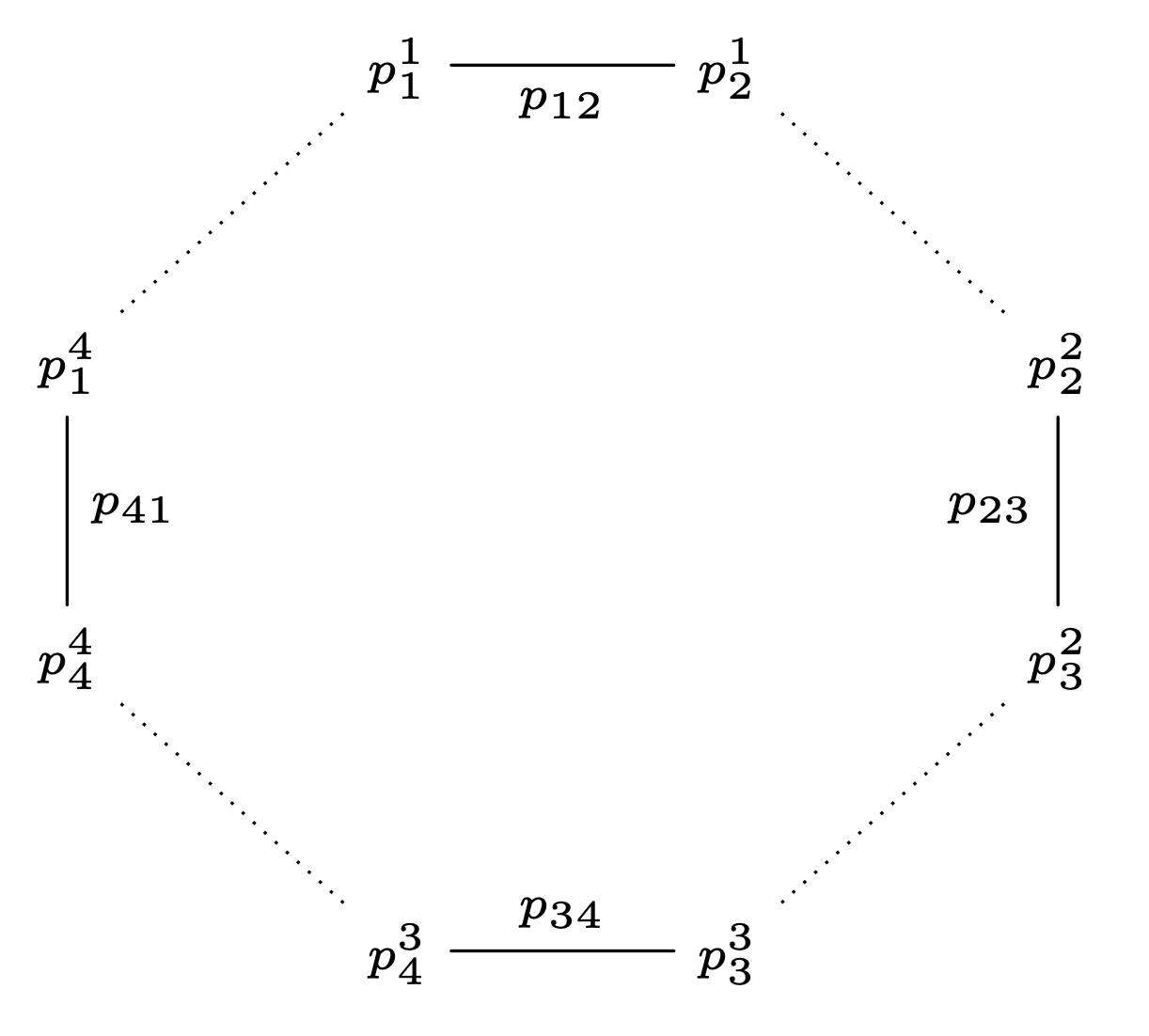
Figure 2: Diagram of all bunch distributions for a rank-4 cyclic system (e.g., the distribution in context $c_{1}$ is described by $p_{1}^{1}=\Pr\left[R_{1}^{1}=1\right]$, $p_{2}^{1}=\Pr\left[R_{2}^{1}=1\right]$, and $p_{12}=\Pr\left[R_{1}^{1}=R_{2}^{1}=1\right]$.)

A cyclic system therefore can be represented by two column vectors:

$$\mathbf{p_{l}}=\left(1,p_{1}^{1},p_{2}^{1}\ldots,p_{n}^{n},p_{1}^{n}\right)^{\intercal},$$ (6)

which is the vector of single-variable expectations preceded by $\left\langle\right\rangle=1$ (the index $\mathbf{l}$ stands for “low-level marginals”), and

$$\mathbf{p_{b}}=\left(p_{12},p_{23},\ldots,p_{n-1,n},p_{n1}\right)^{\intercal},$$ (7)

the vector of all bunch product expectations.

A coupling of a connection $\left\{R_{i}^{i},R_{i}^{i\ominus 1}\right\}$ is a pair of jointly distributed random variables $\left\{T_{i}^{i},T_{i}^{i\ominus 1}\right\}$ with the same 1-marginals:

$$\begin{array}[]{c}\left\langle T_{i}^{i}\right\rangle=\left\langle R_{i}^{i}\right\rangle=p_{i}^{i},\\ \left\langle T_{i}^{i\ominus 1}\right\rangle=\left\langle R_{i}^{i\ominus 1}\right\rangle=p_{i}^{i\ominus 1}.\end{array}$$ (8)

In other words, a coupling adds to each pair $p_{i}^{i},p_{i}^{i\ominus 1}$ describing the connection a product expectation

$$\left\langle T_{i}^{i}T_{i}^{i\ominus 1}\right\rangle=p^{i,i\ominus 1}=\Pr\left[T_{i}^{i}=T_{i}^{i\ominus 1}=1\right],$$ (9)

as it is shown in Fig. 3. This can generally be done in an infinity of ways, constrained only by

$$\max\left(0,p_{i}^{i}+p_{i}^{i\ominus 1}-1\right)\leq p^{i,i\ominus 1}\leq\min\left(p_{i}^{i},p_{i}^{i\ominus 1}\right).$$ (10)

If couplings are constructed for all connections, they are represented by a vector of connection product expectations,

$$\mathbf{p_{c}}=\left(p^{1n},p^{21},p^{32},\ldots,p^{n,n-1}\right)^{\intercal}.$$ (11)

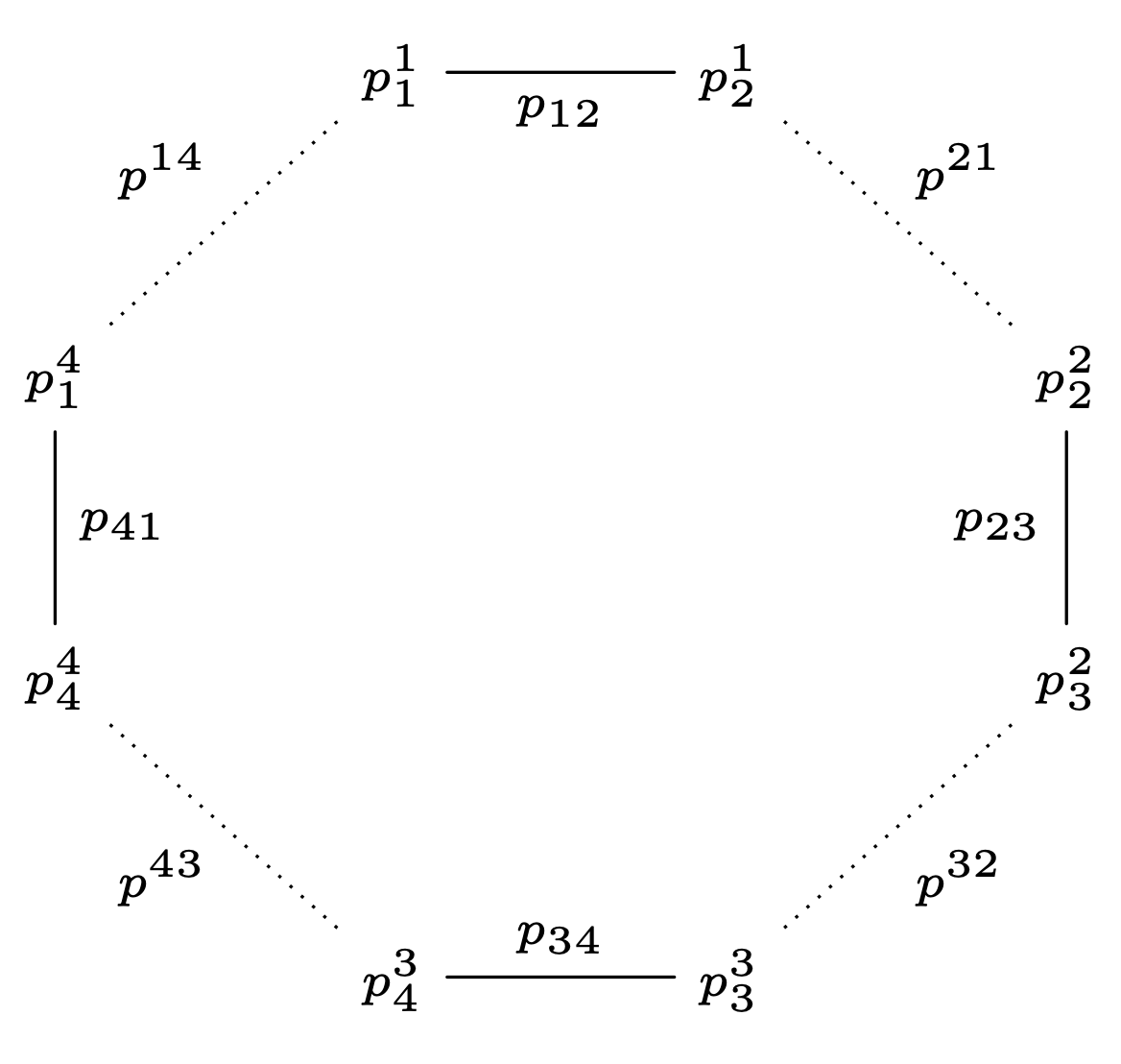
Figure 3: The same diagram as in Fig. 2, complemented with coupling distributions for the connections (e.g., for the coupling of the connection corresponding to $q_{1}$ the distribution is described by $p_{1}^{1}=\Pr\left[T_{1}^{1}=1\right]=\Pr\left[R_{1}^{1}=1\right]$, $p_{1}^{4}=\Pr\left[T_{1}^{4}=1\right]=\Pr\left[R_{1}^{4}=1\right]$, and $p^{14}=\Pr\left[T_{1}^{1}=T_{1}^{4}=1\right]$).

An (overall) coupling of the entire system $\mathcal{R}$ is a set

$$\mathcal{S}=\left\{S_{j}^{i}:j=i,i\oplus 1;i=1,\ldots,n\right\}$$ (12)

of jointly distributed random variables such that, for $i=1,\ldots,n$,

$$\begin{array}[]{c}\left\langle S_{i}^{i}\right\rangle=\left\langle R_{i}^{i}\right\rangle=p_{i}^{i},\\ \left\langle S_{i\oplus 1}^{i}\right\rangle=\left\langle R_{i\oplus 1}^{i}\right\rangle=p_{i\oplus 1}^{i},\\ \left\langle S_{i}^{i}S_{i\oplus 1}^{i}\right\rangle=\left\langle R_{i}^{i}R_{i\oplus 1}^{i}\right\rangle=p_{i,i\oplus 1}.\end{array}$$ (13)

In other words, a coupling $\mathcal{S}$ induces as its 1-marginals and 2-marginals the same vectors $\mathbf{p_{l}},\mathbf{p_{b}}$ as those representing $\mathcal{R}$. An overall coupling also induces couplings of all connections as its 2-marginals $\left(S_{i}^{i},S_{i}^{i\ominus 1}\right)$, which means that it induces a vector $\mathbf{p_{c}}$ of connection product expectations.

III (Non)contextuality

In the following it is convenient to speak of cyclic systems as represented by vectors

$$\mathbf{p}=\left(\begin{array}[]{c}\mathbf{p_{l}}\\ \mathbf{p_{b}}\\ \mathbf{p_{c}}\end{array}\right),$$ (14)

even though $\mathbf{p_{c}}$ is computed and added to a given system. Since this can be done in multiple ways, one and the same system is represented by multiple vectors $\mathbf{p}$.

If in a vector $\mathbf{p_{c}}$,

$$p^{i,i\ominus 1}=\min\left(p_{i}^{i},p_{i}^{i\ominus 1}\right),i=1,\ldots,n,$$ (15)

then the values of $p^{i,i\ominus 1}$ are maximal possible ones, and the couplings of the connections used to compute these product expectations are called maximal couplings. In particular, if the system is consistently connected, i.e.,

$$p_{i}^{i}=p_{i}^{i\ominus 1}=p_{i},i=1,\ldots,n,$$ (16)

then the joint and marginal probabilities in the maximal coupling are as shown,

$$\begin{array}[]{c||c|c||c}\textnormal{probability of}&T_{i}^{i}=1&T_{i}^{i}=0\\ \hline\cr\hline\cr T_{i}^{i\ominus 1}=1&p_{i}&0&p_{i}\\ \hline\cr T_{i}^{i\ominus 1}=0&0&1-p_{i}&1-p_{i}\\ \hline\cr\hline\cr&p_{i}&1-p_{i}\end{array}\>,$$ (17)

whence

$$\Pr\left[T_{i}^{i}\not=T_{i}^{i\ominus 1}\right]=0,i=1,\ldots,n.$$ (18)

In other words, in a consistently connected system the random variables in each connection are treated as if they were essentially the same random variable. In the general case, with $p_{i}^{i}$ and $p_{i}^{i\ominus 1}$ not necessarily equal, it is easy to show that

$$\Pr\left[T_{i}^{i}\not=T_{i}^{i\ominus 1}\right]=\left|p_{i}^{i}-p_{i}^{i\ominus 1}\right|,i=1,\ldots,n.$$ (19)

That is, the maximal coupling $\left\{T_{i}^{i},T_{i}^{i\ominus 1}\right\}$ of $\left\{R_{i}^{i},R_{i}^{i\ominus 1}\right\}$ provides a natural measure of difference between the two variables (in fact, it is the total variation distance between them). The intuitive meaning of contextuality can be presented in the form of the following counterfactual: if all the random variables in the system containing pairs $R_{i}^{i}$ and $R_{i}^{i\ominus 1}$ were jointly distributed, it would force some of these pairs (measuring “the same thing” in different contexts) to be more dissimilar than they are in isolation.

Let us agree that an observed, or target system $\mathcal{R}$ (one being investigated) is represented by the vector

$$\mathbf{p^{*}}=\left(\begin{array}[]{c}\mathbf{p_{l}^{*}}\\ \mathbf{p_{b}^{*}}\\ \mathbf{p_{c}^{*}}\end{array}\right),$$ (20)

where $\mathbf{p_{l}^{*}}$ and $\mathbf{p_{b}^{*}}$ are as they are observed, and $\mathbf{p_{c}^{*}}$ is the vector of the maximal connection product expectations.

Definition 1.

A target system $\mathcal{R}$ represented by vector $\left(\mathbf{p_{l}^{*}},\mathbf{p_{b}^{*}},\mathbf{p_{c}^{*}}\right)^{\intercal}$ is noncontextual if it has a coupling $\mathcal{S}$ that induces as its marginals the vector $\mathbf{p_{c}^{*}}$ (of maximal connection product expectations). If no such coupling exists, the system is contextual.

In other words, if a system is noncontextual it has an overall coupling that (by definition) satisfies (13), and also

$$\left\langle S_{i}^{i}S_{i}^{i\ominus 1}\right\rangle=p^{i,i\ominus 1}=\min\left(p_{i}^{i},p_{i}^{i\ominus 1}\right),i=1,\ldots,n.$$ (21)

In the case of consistent connectedness, CbD essentially reduces to the conventional contextuality analysis (see Refs. (DzhKujFoundations2017, ) and (Dzh2019, ) for logical ramifications of this reduction). As an example, for a consistently connected cyclic system of rank 3,

$$\begin{array}[]{|c|c|c||c|}\hline\cr R_{1}^{1}&R_{2}^{1}&&c^{1}\\ \hline\cr&R_{2}^{2}&R_{3}^{2}&c^{2}\\ \hline\cr R_{1}^{3}&&R_{3}^{3}&c^{3}\\ \hline\cr\hline\cr q_{1}&q_{2}&q_{3}&\mathcal{R}_{3}\\ \hline\cr\end{array},$$ (22)

if it is noncontextual, its coupling satisfying Definition 1, due to (18), can be presented as

$$\begin{array}[]{|c|c|c||c|}\hline\cr S_{1}&S_{2}&&c^{1}\\ \hline\cr&S_{2}&S_{3}&c^{2}\\ \hline\cr S_{1}&&S_{3}&c^{3}\\ \hline\cr\hline\cr q_{1}&q_{2}&q_{3}&\mathcal{S}_{3}\\ \hline\cr\end{array},$$ (23)

involving just three random variables recorded two at a time.

Let

$$\mathbf{M=\left(\begin{array}[]{c}\mathbf{M_{l}}\\ \mathbf{M_{b}}\\ \mathbf{M_{c}}\end{array}\right)}$$ (24)

be a Boolean (incidence) matrix with $0/1$ cells. The $2^{2n}$ columns of $\mathbf{M}$ are indexed by events

$$S_{1}^{1}=r_{1}^{1},S_{2}^{1}=r_{2}^{1},\ldots,S_{n}^{n}=r_{n}^{n},S_{1}^{n}=r_{1}^{n},$$ (25)

while its rows are indexed by the elements of $\mathbf{p}$ (with $\mathbf{M_{l}}$ corresponding to $\mathbf{p_{l}}$, $\mathbf{M_{b}}$ to $\mathbf{p_{b}}$, and $\mathbf{M_{c}}$ to $\mathbf{p_{c}}$). A cell $\left(l,m\right)$ of $\mathbf{M}$ is filled with 1 if the following is satisfied: for each random variable $S_{j}^{i}$ entering the expectation that indexes the $l$th row of $\mathbf{M}$, the value of $S_{j}^{i}$ in the event indexing the $m$th column of $\mathbf{M}$ is equal to 1. Otherwise the cell is filled with zero. For instance, if the $l$th row of $\mathbf{M}$ corresponds to the expectation $\left\langle S_{1}^{1}S_{1}^{2}\right\rangle$ in $\mathbf{p}$, we put 1 in the cell $\left(l,m\right)$ if both $r_{1}^{1}$ and $r_{1}^{2}$ in the event (25) corresponding to the $m$th column of $\mathbf{M}$ are 1; otherwise the cell is filled with zero.

Once $\mathbf{p^{*}}$and $\mathbf{M}$ are defined, one can reformulate the definition of (non)contextuality as follows.

Definition 2 (equivalent to Definition 1).

A target system $\mathcal{R}$ represented by vector $\mathbf{p^{*}=\left(\mathbf{p_{l}^{*}},\mathbf{p_{b}^{*}},\mathbf{p_{c}^{*}}\right)^{\intercal}}$ is noncontextual if and only if there is a vector $\mathbf{h}\geq 0$ (componentwise) such that

$$\mathbf{M}\mathbf{\mathbf{h}}=\mathbf{p^{*}}.$$ (26)

Otherwise the system is contextual.

It is easy to show that if such a vector $\mathbf{h}$ exists, then it can always be interpreted as the column-vector of probabilities

$$\Pr\left[S_{1}^{1}=r_{1}^{1},S_{2}^{1}=r_{2}^{1},\ldots,S_{n}^{n}=r_{n}^{n},S_{1}^{n}=r_{1}^{n}\right]$$

for some overall coupling $\mathcal{S}$ of a system, across all $2^{2n}$ combinations of $r_{j}^{i}=0/1$. In particular, the elements of $\mathbf{h}$ sum to 1, because the first row of $\mathbf{M}$ and the first element of $\mathbf{p^{*}}$ consist of 1’s only.

IV Relabeling from $0/1$ to $\pm 1$

For many aspects of cyclic systems it is more convenient to label the values of the random variables $\pm 1$ rather than consider them Bernoulli, $0/1$. This amounts to switching from $R_{j}^{i}$ variables to $A_{j}^{i}=2R_{j}^{i}-1$. In the case of the connection couplings (8), this means switching from $T_{j}^{i}$ to $U_{j}^{i}=2T_{j}^{i}-1$. A cyclic system $\mathcal{R}$ with Bernoulli variables will then be renamed into a cyclic system $\mathcal{A}$ with $\pm 1$-variables. We have, for $i=1,\ldots,n$,

$$\begin{array}[]{c}\left\langle A_{j}^{i}\right\rangle=e_{j}^{i}=2p_{j}^{i}-1,j=i,i\oplus 1,\\ \left\langle A_{i}^{i}A_{i\oplus 1}^{i}\right\rangle=e_{i,i\oplus 1}=4p_{i,i\oplus 1}-2p_{i}^{i}-2p_{i\oplus 1}^{i}+1,\\ \left\langle U_{i}^{i}U_{i}^{i\ominus 1}\right\rangle=e^{i,i\ominus 1}=4p^{i,i\ominus 1}-2p_{i}^{i}-2p_{i}^{i\ominus 1}+1,\end{array}$$ (27)

and this defines componentwise the transformation of the expectation vectors

$$\left(\begin{array}[]{c}\mathbf{e_{l}}\\ \mathbf{e_{b}}\\ \mathbf{e_{c}}\end{array}\right)=\phi\left(\begin{array}[]{c}\mathbf{p_{l}}\\ \mathbf{p_{b}}\\ \mathbf{p_{c}}\end{array}\right).$$ (28)

The relabeling in question is useful in the formulation of the Bell-type criterion of noncontextuality. Let us denote

$$s_{1}\left(\mathbf{e_{b}}\right)=\max_{\begin{array}[]{c}\lambda_{i}=\pm 1,i=1,\ldots,n\\ \prod_{i=1}^{n}\lambda_{i}=-1\end{array}}\sum\lambda_{i}e_{i,i\oplus 1},$$ (29)

$$\delta\left(\mathbf{e_{l}}\right)=\sum_{i=1}^{n}\left|e_{i}^{i}-e_{i}^{i\ominus 1}\right|.$$ (30)

and

$$\Delta\left(\mathbf{e_{l}}\right)=\min\left(n-2+\delta\left(\mathbf{e_{l}}\right),n\right).$$ (31)

Note that $\delta$ and $\Delta$ depend on $\mathbf{e_{l}}$, but since this vector is fixed, we may (and will henceforth) consider $\delta$ and $\Delta$ as constants (footnote3, ).

Theorem 3 (Kujala-Dzhafarov (KujDzhProof2016, )).

A cyclic system $\mathcal{A}$ represented by vector $\left(\mathbf{e_{l}^{*}},\mathbf{e_{b}^{*}},\mathbf{e_{c}^{*}}\right)^{\intercal}$ is noncontextual if and only if

$$s_{1}\left(\mathbf{e_{b}^{*}}\right)-\Delta\leq 0.$$ (32)

This result generalizes the criterion derived in Ref. (Araujoetal2013, ) for consistently connected cyclic systems (those with $\delta=0$).

V Measures of contextuality and a measure of noncontextuality

The idea of the two measures of contextuality considered in Ref. (KujDzhMeasures, ), $\textnormal{CNT}_{1}$ and $\textnormal{CNT}_{2}$, is as follows. First we think of the space of all $\mathbf{p}=\left(\mathbf{p_{l}},\mathbf{p_{b}},\mathbf{p_{c}}\right)^{\intercal}$ obtainable as $\mathbf{p}=\mathbf{Mh}$ with $\mathbf{h}\geq 0$. In this space, we fix the 1-marginals $\mathbf{p_{l}}$ at $\mathbf{p_{l}^{*}}$ (observed values), and define the polytope

$$\mathbb{P}=\left\{\mathbf{\left.\left(\begin{array}[]{c}\mathbf{p_{b}}\\ \mathbf{p_{c}}\end{array}\right)\right|}\exists\mathbf{h}\geq 0:\left(\begin{array}[]{c}\mathbf{p_{l}^{*}}\\ \mathbf{p_{b}}\\ \mathbf{p_{c}}\end{array}\right)=\left(\begin{array}[]{c}\mathbf{M_{l}}\\ \mathbf{M_{b}}\\ \mathbf{M_{c}}\end{array}\right)\mathbf{h}\right\}.$$ (33)

This polytope describes all possible couplings of all systems with low-marginals $\mathbf{p_{l}^{*}}$. Then we do one of the two: either we fix $\mathbf{M_{b}h}=\mathbf{p_{b}^{*}}$ and see how close $\mathbf{p_{c}=M_{c}h}$ can be made to $\mathbf{p_{c}^{*}}$ by changing $\mathbf{h}$; or we fix $\mathbf{M_{c}h}=\mathbf{p_{c}^{*}}$ and see how close $\mathbf{p_{b}=M_{b}h}$ can be made to $\mathbf{p_{b}^{*}}$. These two procedures define two polytopes that we use to define $\textnormal{CNT}_{1}$ and $\textnormal{CNT}_{2}$, respectively.

Definition 4.

If a system $\mathcal{R}$ represented by vector $\mathbf{p}^{*}$ is contextual,

$$\textnormal{CNT}_{1}=L_{1}\left(\mathbf{p_{c}^{*}},\mathbb{P}_{\mathbf{c}}\right)$$ (34)

the $L_{1}$-distance between $\mathbf{p_{c}^{*}}$ and the feasibility polytope

$$\mathbb{P}_{\mathbf{c}}=\left\{\left.\begin{array}[]{c}\\ \\ \end{array}\mathbf{p_{c}}\right|\exists\mathbf{h}\geq 0:\left(\begin{array}[]{c}\mathbf{p_{l}^{*}}\\ \mathbf{p_{b}^{*}}\\ \mathbf{p_{c}}\end{array}\right)=\left(\begin{array}[]{c}\mathbf{M_{l}}\\ \mathbf{M_{b}}\\ \mathbf{M_{c}}\end{array}\right)\mathbf{h}\right\}.$$ (35)

Written in extenso,

$$\textnormal{CNT}_{1}=\min_{\mathbf{p_{c}}\in\mathbb{P}_{\mathbf{c}}}\left\|\mathbf{p_{c}^{*}}-\mathbf{p_{c}}\right\|_{1}=\mathbf{1}\cdot\mathbf{p_{c}^{*}}-\max_{\mathbf{p_{c}}\in\mathbb{P}_{\mathbf{c}}}\left(\mathbf{1}\cdot\mathbf{p_{c}}\right).$$ (36)

Because $\mathbf{p_{l}}$ is fixed at $\mathbf{p_{l}^{*}}$, the transformation $\phi$ in (28) has the form $4p^{i,i\ominus 1}+\textnormal{const}$ for each component of $\mathbf{p_{c}}$, and we have

$$\left\|\mathbf{p_{c}^{*}}-\mathbf{p_{c}}\right\|_{1}=\frac{\left\|\mathbf{e_{c}^{*}}-\mathbf{e_{c}}\right\|_{1}}{4}.$$ (37)

This allows us to redefine the measure in the way more convenient for our purposes,

$$\textnormal{CNT}_{1}=\frac{1}{4}L_{1}\left(\mathbf{e_{c}^{*}},\mathbb{E}_{\mathbf{c}}\right),$$ (38)

where (pointwise)

$$\mathbb{E}_{\mathbf{c}}=\phi\left(\mathbb{P}_{\mathbf{c}}\right).$$ (39)

Definition 5.

If a system $\mathcal{R}$ represented by vector $\mathbf{p}^{*}$ is contextual,

$$\textnormal{CNT}_{2}=L_{1}\left(\mathbf{p_{b}^{*}},\mathbb{P}_{\mathbf{b}}\right),$$ (40)

the $L_{1}$-distance between $\mathbf{p_{b}^{*}}$ and the noncontextuality polytope

$$\mathbb{P}_{\mathbf{b}}=\left\{\left.\begin{array}[]{c}\\ \\ \end{array}\mathbf{p_{b}}\right|\exists\mathbf{h}\geq 0:\left(\begin{array}[]{c}\mathbf{p_{l}^{*}}\\ \mathbf{p_{b}}\\ \mathbf{p_{c}^{*}}\end{array}\right)=\left(\begin{array}[]{c}\mathbf{M_{l}}\\ \mathbf{M_{b}}\\ \mathbf{M_{c}}\end{array}\right)\mathbf{h}\right\}.$$ (41)

Here,

$$\textnormal{$\textnormal{CNT}_{2}$}=\min_{\mathbf{p_{b}}\in\mathbb{P}_{\mathbf{b}}}\left\|\mathbf{p_{b}^{*}}-\mathbf{p_{b}}\right\|_{1}.$$ (42)

For the same reason as above, the transformation $\phi$ in (28) has the form $4p_{i,i\oplus 1}+\textnormal{const}$ for each component of $\mathbf{p_{b}}$. We have therefore

$$\textnormal{CNT}_{2}=\frac{1}{4}L_{1}\left(\mathbf{e_{b}^{*}},\mathbb{E}_{\mathbf{b}}\right),$$ (43)

the $L_{1}$-distance between $\mathbf{e_{b}^{*}=\phi\left(p_{b}^{*}\right)}$ and the polytope

$$\mathbb{E}_{\mathbf{b}}=\phi\left(\mathbb{P}_{\mathbf{b}}\right).$$ (44)

For convenience, we will use the same term, “feasibility polytope,” for both $\mathbb{P}_{\mathbf{c}}$ and $\mathbb{E}_{\mathbf{c}}$. Analogously, both $\mathbb{P}_{\mathbf{b}}$ and $\mathbb{E}_{\mathbf{b}}$ can be referred to as “noncontextuality polytope.”

As for any two $\pm 1$-random variables, we have

$$\left|e_{i}^{i}+e_{i\oplus 1}^{i}\right|-1\leq e_{i,i\oplus 1}\leq 1-\left|e_{i}^{i}-e_{i\oplus 1}^{i}\right|,i=1,\ldots,n.$$ (45)

Therefore the convex polytope $\mathbb{E}_{\mathbf{b}}$ is circumscribed by the $n$-box

$$\mathbb{R_{\mathbf{b}}}=\prod_{i=1}^{n}\left[\left|e_{i}^{i}+e_{i\oplus 1}^{i}\right|-1,1-\left|e_{i}^{i}-e_{i\oplus 1}^{i}\right|\right].$$ (46)

We can analogously define the $n$-box circumscribing $\mathbb{E}_{c}$, but we do not need this notion.

The idea of the noncontextuality measure $\textnormal{NCNT}_{2}$ extending $\textnormal{CNT}_{2}$ to noncontextual systems is as follows.

Definition 6.

If a system $\mathcal{R}$ represented by vector $\mathbf{p}^{*}$ is noncontextual,

$$\textnormal{NCNT}_{2}=L_{1}\left(\mathbf{p_{b}^{*}},\partial\mathbb{P}_{\mathbf{b}}\right)=\frac{1}{4}L_{1}\left(\mathbf{e_{b}^{*}},\partial\mathbb{E}_{\mathbf{b}}\right),$$ (47)

the $L_{1}$ distance between $\mathbf{p_{b}^{*}}$ and the surface $\partial\mathbb{P}_{\mathbf{b}}$ of the noncontextuality polytope $\mathbb{P}_{\mathbf{b}}$.

Note that $\textnormal{CNT}_{2}$, too, could be defined as the distance from a point to $\partial\mathbb{P}_{\mathbf{b}}$, so the definition is the same for both $\textnormal{CNT}_{2}$ and $\textnormal{NCNT}_{2}$, only the position of the $\mathbf{p_{b}^{*}}$ changes from the outside to the inside of the polytope. In extenso,

$$\textnormal{$\textnormal{NCNT}_{2}$}=\frac{1}{4}\min_{\mathbf{e_{b}}\in\partial\mathbb{E}_{\mathbf{b}}}\left\|\mathbf{e_{b}^{*}}-\mathbf{e_{b}}\right\|_{1}=\frac{1}{4}\inf_{\mathbf{x}\in\mathbf{R}^{n}-\mathbb{E}_{\mathbf{b}}}\left\|\mathbf{e_{b}^{*}}-\mathbf{x}\right\|_{1},$$ (48)

where $\mathbf{R}$ is the set of reals. As shown in Ref. (KujDzhMeasures, ), no such extension to a noncontextuality measure exists for $\textnormal{CNT}_{1}$ (see Sec. IX for the argument by which this is established).

VI Additional terminology and conventions

To focus now on $\textnormal{CNT}_{2}$ and $\textnormal{NCNT}_{2}$, we need a few additional terms and conventions. We confine our consideration to the space of all possible points $\mathbf{e_{b}}$, which is the n-cube

$$\mathbb{C}_{\mathbf{b}}=\left[-1,1\right]^{n}.$$ (49)

Given an arbitrary $n$-box

$$\mathbb{X}=\prod_{i=1}^{n}\left[\min x_{i},\max x_{i}\right]\subseteq\mathbb{C}_{\mathbf{b}},$$ (50)

a vertex $V$ of $\mathbb{\mathbb{X}}$ is called odd if its coordinates contain an odd number of $\min x_{i}$’s; otherwise the vertex is even. A hyperplane is said to be pocket-forming at vertex $V$ if it cuts each of the $n$ edges emanating from $V$, i.e., if it intersects each of them between $V$ and the edge’s other end. The region within $\mathbb{\mathbb{X}}$ strictly above the pocket-forming hyperplane at $V$ is called a pocket at $V$. This pocket is said to be regular if the pocket-forming hyperplane cuts all $n$ edges emanating from $V$ at an equal distance from $V$. We apply this terminology to two special $n$-boxes: the $n$-box $\mathbb{R}_{\mathbf{b}}$ circumscribing the noncontextuality polytope (46), and the ambient n-cube $\mathbb{C}_{\mathbf{b}}$ itself.

We will assume in the following that no context in the system contains a deterministic variable. If such a context exists, the $n$-box $\mathbb{R}_{\mathbf{b}}$ is degenerate (has lower dimensionality than $n$), and

$$\mathbb{E}_{\mathbf{b}}=\mathbb{R_{\mathbf{b}}},$$

making the system trivially noncontextual. Indeed, assume, e.g., that $A_{1}^{1}$ is a deterministic variable. We know that any deterministic variable can be removed from a system without affecting its (non)contextuality (Dzh2017Nothing, ). The system therefore can be presented as a noncyclic chain

$$A_{2}^{1},A_{2}^{2},A_{3}^{2},\ldots,A_{n}^{n},A_{1}^{n}.$$

Whatever the joint distributions of adjacent pairs in such a chain, there is always a global joint distribution that agrees with these pairwise distributions as its marginals: for any assignment of values to the links of the chain, the coupling probability is obtained as the product of the chained conditional probabilities.

A cyclic system $\mathcal{A}$ is called a variant of a cyclic system $\mathcal{B}$ of the same rank if

$$\left\{A_{i}^{i},A_{i}^{i\ominus 1}\right\}=\pm 1\cdot\left\{B_{i}^{i},B_{i}^{i\ominus 1}\right\},$$ (51)

for $i=1,\ldots,n$.

Lemma 7 (Kujala-Dzhafarov (KujDzhProof2016, )).

All variants of a system have the same values of $s_{1}$$\left(\mathbf{e_{b}}\right)$ and $\left|e_{i}^{i}-e_{i}^{i\ominus 1}\right|$, $i=1,\ldots,n$ (hence also they have the same value of $\Delta$).

Lemma 8 (Kujala-Dzhafarov (KujDzhProof2016, )).

Among the $2^{n}$ variants of a cyclic system there is one, called canonical, in which (following a circular permutation of indices)

$$\left|e_{n1}\right|\leq e_{i,i+1},i=1,\ldots,n-1.$$ (52)

Clearly, a canonical variant of a system is a canonical variant of any variant of the system, including itself. In a canonical variant of a system,

$$s_{1}\left(\mathbf{e_{b}}\right)=\sum_{i=1}^{n-1}e_{i,i+1}-e_{n1}.$$ (53)

VII Properties of the noncontextuality polytope

In this section we present a series of lemmas establishing the remarkably simple structure of the noncontextuality polytope. The proofs of these results are relegated to the Appendix.

Lemma 9.

For each odd vertex $V=\left\{\lambda_{i}:i=1,\ldots,n\right\}$ of $\mathbb{C_{\mathbf{b}}}$, the inequality $\sum\lambda_{i}e_{i,i\oplus 1}>\Delta$ describes a regular pocket at $V$. The distance at which the hyperplane segment $\sum\lambda_{i}e_{i,i\oplus 1}=\Delta$ cuts each of the edges of the cube emanating from $V$ is $n-\Delta$. (See Fig. 4.)

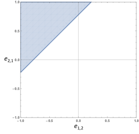
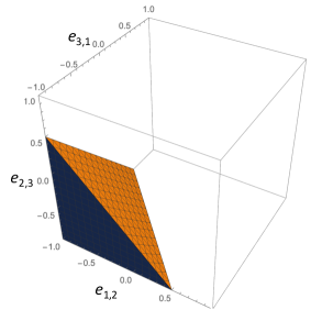
Figure 4: Illustration for Lemma 9, $n=2$ and $n=3$.

Lemma 10.

For a given $\Delta$, no two pockets $\sum\lambda_{i}e_{i,i\oplus 1}>\Delta$ and $\sum\lambda^{\prime}_{i}e_{i,i\oplus 1}>\Delta$ formed by the hyperplanes at different odd vertices of $\mathbb{C_{\mathbf{b}}}$ intersect. The pocket-forming hyperplanes at the odd vertices are also disjoint within $\mathbb{C}_{\mathbf{b}}$ unless $\Delta=n-2$. (See Figs. 5 and 6.)

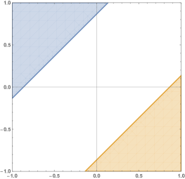
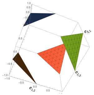
Figure 5: Illustration for Lemma 10, $n=2$ and $n=3$. The pocket-forming hyperplanes at different odd vertices of $\mathbb{C_{\mathbf{b}}}$ do not touch within $\mathbb{C}_{\mathbf{b}}$ when $\Delta>n-2$.

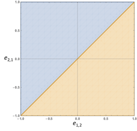
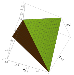
Figure 6: Illustration for Lemma 10 (continued), $n=2$ and $n=3$. When $\Delta=n-2$, the pocket-forming hyperplanes at different odd vertices of $\mathbb{C_{\mathbf{b}}}$ form an $n$-demicube, the convex hull of the $2^{n-1}$ even vertices of $\mathbb{C_{\mathbf{b}}}$.

Lemma 11.

If a point $\mathbf{x}$ is within the pocket formed at an odd vertex $V=\left\{\lambda_{i}:i=1,\ldots,n\right\}$ of $\mathbb{C}_{\mathbf{b}}$ by a hyperplane segment $\sum\lambda_{i}e_{i,i\oplus 1}=\Delta$, then

$$s_{1}\left(\mathbf{x}\right)=\sum\lambda_{i}x_{i,i\oplus 1}=\Delta_{\mathbf{x}}>\Delta,$$

and $s_{1}\left(\mathbf{x}\right)-\Delta$ is the distance between the points at which the two hyperplane segments $\sum\lambda_{i}e_{i,i\oplus 1}=\Delta_{\mathbf{x}}$ and $\sum\lambda_{i}e_{i,i\oplus 1}=\Delta$ cut any of the edges emanating from $V$. (See Fig. 7.)

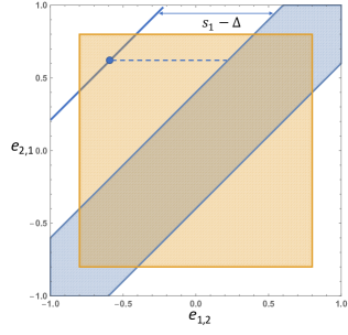
Figure 7: Illustration for Lemma 11, $n=2$, and for subsequent development. The hyperplane segment $\sum\lambda_{i}e_{i,i\oplus 1}=\Delta$ is shown as the left boundary of the extended noncontextuality polytope (here, hexagon) $\mathbb{N}_{\mathbf{b}}$. The smaller internal rectangle represents $\mathbb{R_{\mathbf{b}}}$.

The extended noncontextuality polytope $\mathbb{N_{\mathbf{b}}\subseteq\mathbb{C}_{\mathbf{b}}}$ is defined by $2^{n-1}$ half-space inequalities

$$\sum_{i=1}^{n}\lambda_{i}e_{i,i\oplus 1}\leq\Delta,i=1,\ldots,n,$$ (54)

where $n-2\leq\Delta\leq n$ and $\left\{\lambda:i=1,\ldots,n\right\}$ are odd vertices of $\mathbb{C}_{\mathbf{b}}$ . Therefore we can identify $\mathbb{N}_{\mathbf{b}}$ by the value of $\Delta$, and write $\mathbb{N}_{\mathbf{b}}=\mathbb{N}_{\mathbf{b}}\left(\Delta\right)$. (See Fig. 8.)

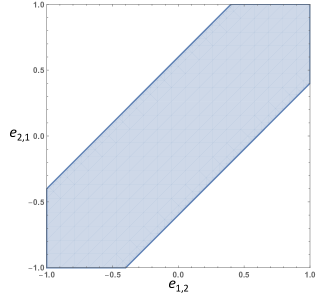
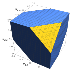
Figure 8: Examples of polytope $\mathbb{N}_{\mathbf{b}}$ within cube $\mathbb{C_{\mathbf{b}}},$ for $n=2$ and $n=3$.

Lemma 12.

If a point $\mathbf{x}$ is within the extended noncontextuality polytope $\mathbb{N}_{\mathbf{b}}\left(\Delta\right)$, then

$$s_{1}\left(\mathbf{x}\right)=\sum\lambda_{i}x_{i,i\oplus 1}=\Delta_{\mathbf{x}}\leq\Delta,$$

where $V=\left\{\lambda:i=1,\ldots,n\right\}$ is an odd vertex of $\mathbb{C}_{\mathbf{b}}$ (unique if $\Delta>n-2$) at which the hyperplane segment $\sum\lambda{}_{i}e_{i,i\oplus 1}=\Delta_{\mathbf{x}}$ forms a pocket. The difference $\Delta-\Delta_{\mathbf{x}}$ is the distance between the points at which the two hyperplanes cut any of the edges emanating from $V$. (See Fig. 9.)

The proof of Lemma 12 is obvious, in view of the previous results.

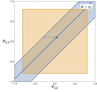
Figure 9: Illustration for Lemma 12, $n=2$. The polytope and the box $\mathbb{R_{\mathbf{b}}}$ are as in Fig. 7.

We know that $\mathbb{E}_{\mathbf{b}}$ is the intersection of $\mathbb{R_{\mathbf{b}}}$ and the polytope $\mathbb{N}_{\mathbf{b}}\left(\Delta\right)$. The following lemma stipulates an important property of this intersection.

Lemma 13.

All even vertices of $\mathbb{R_{\mathbf{b}}}$ are within $\mathbb{E}_{\mathbf{b}}$. (See Fig. 10.)

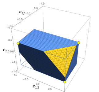
Figure 10: Illustration for Lemma 13, $n=2$ and $n=3$: even vertices are shown by small circles.

Corollary 14.

A point $\mathbf{x}$ represents a contextual system if and only if it belongs to a pocket formed by a pocket-forming hyperplane segment $\sum\lambda_{i}e_{i,i\oplus 1}=\Delta$ at an odd vertex $V=\left\{\lambda_{i}:i=1,\ldots,n\right\}$ of $\mathbb{R}_{\mathbf{b}}$. These pockets are regular and their number is $0\leq k\leq 2^{n-1}$. (See Fig. 11.)

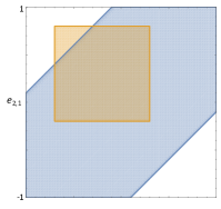
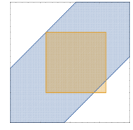
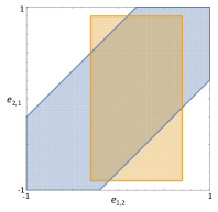
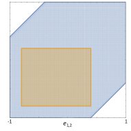
Figure 11: Illustration for Corollary 14, $n=2$. The number of regular pockets formed at odd vertices of box $\mathbb{R}_{\mathbf{b}}$ can be 1 (upper panels), 2 (left lower), or zero (right lower).

VIII Main theorems

The following two theorems now are simple corollaries of the previous results. Consider a noncontextuality polytope

$$\mathbb{E}_{\mathbf{b}}=\mathbb{R}_{\mathbf{b}}\cap\mathbb{N}_{\mathbf{b}}\left(\Delta\right).$$ (55)

Theorem 15.

The $L_{1}$-distance between $\mathbb{E}_{\mathbf{b}}$ and a point $\mathbf{e_{b}^{*}}$ representing a contextual system is a single-coordinate distance, equal to $s_{1}\left(\mathbf{e_{b}^{*}}\right)-\Delta$ for all coordinates. This is the value of 4$\cdot$$\textnormal{CNT}_{2}$. (See Fig. 12.)

Figure 12: Illustration for Theorem 15, $n=2$, a detailed analog of Fig. 1A.

It is easy to show that for any $p\geq 1$, the $\frac{1}{4}$ of the $L_{p}$-distance between $\mathbf{e_{b}^{*}}$ and $\mathbb{E}_{\mathbf{b}}$ (let us call it $\textnormal{CNT}_{2}^{\left(p\right)}$) is simply

$$\textnormal{CNT}_{2}^{\left(p\right)}=n^{\frac{1-p}{p}}\textnormal{CNT}_{2},$$ (56)

where $n$ is the rank of the cyclic system. This means that in the case of contextual cyclic systems $L_{1}$-distance can be, if one so wishes, replaced by any $L_{p}$-distance with no nontrivial changes in the theory. However, this may not be possible for noncyclic systems, where the faces of the noncontextuality polytope need not have the simple structure of $\mathbb{E}_{\mathbf{b}}$.

Let us define a new measure now, the $L_{1}$-distance between the box $\mathbb{R}_{\mathbf{b}}$ and a point $\mathbf{e_{b}}$ within the box:

$$m\left(\mathcal{\mathbf{\mathbf{e_{b}}}}\right)=\min_{i=1,\ldots,n}\left(\min\left(\begin{array}[]{c}e_{i,i\oplus 1}-\left|e_{i}+e_{i\oplus 1}\right|+1,\\ 1-\left|e_{i}^{i}-e_{i\oplus 1}^{i}\right|-e_{i,i\oplus 1}\end{array}\right)\right).$$ (57)

Theorem 16.

The $L_{1}$-distance between the surface of $\mathbb{E}_{\mathbf{b}}$ and a point $\mathbf{\mathbf{e_{b}^{*}}}$ representing a noncontextual system is a single-coordinate distance, equal to $\min\left(\Delta-s_{1}\left(\mathbf{\mathbf{\mathbf{e_{b}^{*}}}}\right),m\left(\mathbf{\mathbf{e_{b}^{*}}}\right)\right)$. This is the value of $4\cdot\textnormal{$\textnormal{NCNT}_{2}$}$. If this value equals $s_{1}\left(\mathbf{e^{*}}\right)-\Delta,$ it is the same for all coordinates. (See Fig. 13.)

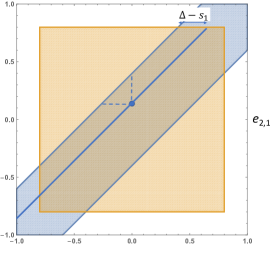
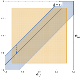
Figure 13: Illustration for Theorem 16, $n=2$, a detailed analog of Figs. 1B and 1C. Upper panel: the case $\Delta-s_{1}\left(\mathbf{\mathbf{\mathbf{e_{b}^{*}}}}\right)\leq m\left(\mathbf{\mathbf{e_{b}^{*}}}\right)$. Lower panel: the case $\Delta-s_{1}\left(\mathbf{e_{b}^{*}}\right)>m\left(\mathbf{e_{b}^{*}}\right)$.

By geometric considerations, $m\left(\mathcal{\mathbf{\mathbf{e_{b}}}}\right)$ is also an $L_{p}$-distance between $\mathbb{R}_{\mathbf{b}}$ and $\mathbf{\mathbf{\mathbf{e_{b}^{*}}}}$, for any $p\geq 1$. Because of this, using the same reasoning as in the case of $\textnormal{CNT}_{2}^{\left(p\right)}$, the $L_{p}$-distance from $\mathbf{\mathbf{\mathbf{e_{b}^{*}}}}$ to the surface of $\mathbb{E}_{\mathbf{b}}$ is

$$\textnormal{NCNT}_{2}^{\left(p\right)}=\frac{1}{4}\min\left(n^{\frac{1-p}{p}}\left(\Delta-s_{1}\left(\mathbf{\mathbf{\mathbf{e_{b}^{*}}}}\right)\right),m\left(\mathbf{\mathbf{e_{b}^{*}}}\right)\right).$$ (58)

As we see, unlike in the case of $\textnormal{CNT}_{2}^{\left(p\right)}$, this is not simply a scaled version of $\textnormal{NCNT}_{2}$, indicating that replacing the latter with $\textnormal{NCNT}_{2}^{\left(p\right)}$ is not inconsequential for the theory.

Figures 14 and 15 illustrate the dynamics of $\textnormal{CNT}_{2}$ and $\textnormal{NCNT}_{2}$ as point $\mathbf{\mathbf{\mathbf{e_{b}^{*}}}}$ moves along the diagonal connecting two opposite vertices of $\mathbb{R}_{\mathbf{b}}$ for cyclic systems of several ranks. To emphasize that $\textnormal{NCNT}_{2}$ is an extension of $\textnormal{CNT}_{2}$ (and vice versa), we plot $\textnormal{NCNT}_{2}$ with minus sign: as $\mathbf{\mathbf{\mathbf{e_{b}^{*}}}}$ moves closer to the surface of $\mathbb{E}_{\mathbf{b}}$, $\textnormal{CNT}_{2}$ decreases from a positive value to zero, the system becomes noncontextual, and as the point continues to move inside the polytope, the value of $-\textnormal{NCNT}_{2}$ proceeds to decrease continuously.

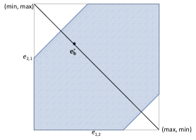
Figure 14: $\textnormal{CNT}_{2}$ (solid lines, positive values) and $-\textnormal{NCNT}_{2}$ (dotted or dashed lines, nonpositive values) as a function of the position of $\mathbf{\mathbf{e_{b}^{*}}}$ on the diagonal connecting two opposite vertices of $\mathbb{R}_{\mathbf{b}}$ for cyclic systems of ranks 2, 4, 6. The dashed lines show the cases $\Delta-s_{1}\left(\mathbf{\mathbf{\mathbf{e_{b}^{*}}}}\right)>m\left(\mathbf{\mathbf{e_{b}^{*}}}\right)$, when $\textnormal{$\textnormal{NCNT}_{2}$}=\frac{1}{4}m\left(\mathbf{\mathbf{e_{b}^{*}}}\right)$; the dotted lines show the case $\Delta-s_{1}\left(\mathbf{\mathbf{\mathbf{e_{b}^{*}}}}\right)\leq m\left(\mathbf{\mathbf{e_{b}^{*}}}\right)$, when $\textnormal{$\textnormal{NCNT}_{2}$}=\frac{1}{4}\left(\Delta-s_{1}\left(\mathbf{\mathbf{\mathbf{e_{b}^{*}}}}\right)\right)$. The lower set of graphs represents inconsistently connected systems, with $\left\langle A_{i}^{i}\right\rangle=-0.2,\left\langle A_{i}^{i\ominus 1}\right\rangle=0.1$, for $i=1,\ldots,n$. The upper graphs represent consistently connected systems, with the expectations of all random variables equal to zero. As indicated in the illustration on the top, for the even-ranked systems, it connects the vertex whose last coordinate is its single min-coordinate to the vertex whose last coordinate is its single max-coordinate.

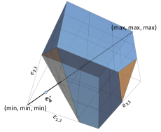
Figure 15: The same as Fig. 14, but for cyclic systems of ranks 3, 5, 7. As indicated in the illustration on the top, for the odd-ranked systems, the diagonal connects the vertex with all min-coordinates to the vertex with all max-coordinates.

IX Polytope of all possible couplings

We now need to gain insight into why $\textnormal{CNT}_{1}$ and $\textnormal{CNT}_{2}$ are the same for cyclic systems. Is it a peculiar coincidence? Does $\textnormal{CNT}_{1}$, if interpreted geometrically, have the same “nice” properties as $\textnormal{CNT}_{2}$? The answer to the first question turns out to be negative, and to second one affirmative.

In Sec. V we introduced in (33) the polytope $\mathbb{P}$ of all possible couplings for a system with the low-marginals $\mathbf{p_{l}^{*}}$. As in the cases of $\mathbb{P}_{\mathbf{b}}$ and $\mathbb{P}_{\mathbf{c}}$, we redefine this polytope in terms of $\pm 1$-variables,

$$\mathbb{E}=\phi\left(\mathbb{P}\right),$$ (59)

and use it to define a measure of contextuality

$$\textnormal{CNT}_{0}=L_{1}\left(\mathbf{\mathbf{\left(\begin{array}[]{c}\mathbf{p_{b}^{*}}\\ \mathbf{p_{c}^{*}}\end{array}\right)}},\mathbb{P}\right)=\frac{1}{4}L_{1}\left(\mathbf{\mathbf{\left(\begin{array}[]{c}\mathbf{e_{b}^{*}}\\ \mathbf{e_{c}^{*}}\end{array}\right)}},\mathbb{E}\right).$$ (60)

To investigate the properties of $\mathbb{E}$ and $\textnormal{CNT}_{0}$ we use the following result:

Theorem 17 (Kujala-Dzhafarov-Larsson (KujDzhLar2015, )).

A system represented by $\left(\mathbf{e_{b}^{*}},\mathbf{e_{c}^{*}}\right)^{\intercal}$ is noncontextual if and only if

$$s_{1}\left(\mathbf{e_{b}^{*}},\mathbf{e_{c}^{*}}\right)\leq 2n-2.$$

This can be understood as a special case of Theorem 3 if one uses the procedure of treating connections as if they were additional contexts, rendering thereby any system consistently connected (KujDzhMeasures, ; AmaralDuarteOliveira2018, ). Here and in the following we write $s_{1}\left(\mathbf{e_{b}^{*}},\mathbf{e_{c}^{*}}\right)$ instead of the more correct $s_{1}\left(\left(\mathbf{e_{b}^{*}},\mathbf{e_{c}^{*}}\right)^{\intercal}\right)$.

It is evident now that the entire development in Secs. VI and V can be repeated with $\mathbb{E}$ replacing $\mathbb{E}_{\mathbf{b}}$, except that the ambient cube $\mathbb{C}$, extended noncontextuality polytope $\mathbb{N}$, and the box $\mathbb{R}$ circumscribing $\mathbb{E}$ (replacing, respectively, $\mathbb{C}_{\mathbf{b}}$, $\mathbb{N}_{\mathbf{b}}$, and $\mathbb{R}_{\mathbf{b}}$) are $2n$-dimensional rather than $n$-dimensional, and the value of $\Delta$ that defines the polytope is $2n-2$. In particular, the shape of the polytope $\mathbb{N}$ is always a $2n$-demicube, the convex hull of the $2^{2n-1}$ even vertices of $\mathbb{C}$, similar to the $n$-demicubes shown in Fig. 6, except that the minimal meaningful number of dimensions has to be 4 (representing a cyclic system of rank 2). The following analog of Theorem 15 then holds.

Theorem 18.

The $L_{1}$-distance between $\mathbb{E}$ and a point $\mathbf{\left(\mathbf{\mathbf{e_{b}^{*}},\mathbf{e_{c}^{*}}}\right)^{\intercal}}$ representing a contextual system is a single-coordinate distance, equal to $s_{1}\left(\mathbf{\mathbf{\mathbf{e_{b}^{*}},\mathbf{e_{c}^{*}}}}\right)-\left(2n-2\right)$ for all coordinates. This is the value of $\textnormal{$\textnormal{CNT}_{0}$}\cdot 4$.

It is easy to see now that

$$\textnormal{$\textnormal{CNT}_{0}$}=\textnormal{$\textnormal{CNT}_{1}$}=\textnormal{$\textnormal{CNT}_{2}$}.$$ (61)

Indeed, the single-coordinate $L_{1}$-distance mentioned in the theorem can be taken along an $\mathbf{e_{b}}$-coordinate or along an $\mathbf{e_{c}}$-coordinate, and with all other coordinates being fixed at appropriate values, this will be a single-coordinate $L_{1}$-distance from, respectively, $\mathbb{E}_{\mathbf{b}}$ or $\mathbb{E}_{\mathbf{c}}$. Since we know that

$$\textnormal{$\textnormal{CNT}_{1}$}=\textnormal{$\textnormal{CNT}_{2}$}=\frac{1}{4}\left(s_{1}\left(\mathbf{\mathbf{e_{b}^{*}}}\right)-\Delta\right),$$ (62)

and that

$$\textnormal{$\textnormal{CNT}_{0}$}=\frac{1}{4}\left(s_{1}\left(\mathbf{\mathbf{\mathbf{e_{b}^{*}},\mathbf{e_{c}^{*}}}}\right)-\left(2n-2\right)\right),$$ (63)

we have an indirect proof that when $s_{1}\left(\mathbf{\mathbf{\mathbf{e_{b}^{*}},\mathbf{e_{c}^{*}}}}\right)>\left(2n-2\right)$ (i.e., the system is contextual),

$$s_{1}\left(\mathbf{\mathbf{e_{b}^{*}},\mathbf{e_{c}^{*}}}\right)=s_{1}\left(\mathbf{\mathbf{e_{b}^{*}}}\right)+n-\delta.$$ (64)

Note that $\textnormal{CNT}_{0}$, like $\textnormal{CNT}_{1}$ and unlike $\textnormal{CNT}_{2}$, cannot be naturally extended to a noncontextuality measure. Because $\mathbf{e_{c}^{*}}$ consists of the maximal possible values of $e^{i,i\oplus 1}$ ($i=1,\ldots,n$), any point $\mathbf{\left(\mathbf{\mathbf{e_{b}^{*}},\mathbf{e_{c}^{*}}}\right)^{\intercal}}$ representing a noncontextual system should lie on the surface of the polytope $\mathbb{E}$, yielding

$$s_{1}\left(\mathbf{\mathbf{\mathbf{e_{b}^{*}},\mathbf{e_{c}^{*}}}}\right)-\left(2n-2\right)=0.$$ (65)

The argument leading to this conclusion was presented in Ref. (KujDzhMeasures, ) for $\mathbb{E}_{\mathbf{c}}$. When applied to $\mathbb{E}$, it goes as follows: if $\mathbf{\mathbf{\mathbf{\left(\mathbf{\mathbf{e_{b}^{*}},\mathbf{e_{c}^{*}}}\right)^{\intercal}}}}$ were an interior point of $\mathbb{E}$, it would be surrounded by a $2n$-ball entirely within $\mathbb{E}$, and one would be able to increase any component of $\mathbf{e_{c}^{*}}$ while remaining within this ball, which is not possible. $\textnormal{CNT}_{2}$ remains the only one of the contextuality measures considered in the literature that can be naturally extended into a noncontextuality measure.

X Conclusion with a glimpse into noncyclic systems

Most of the regularities established in this paper do not generalize to noncyclic systems. In particular, $\textnormal{CNT}_{1}$ and $\textnormal{CNT}_{2}$ do not generally coincide, nor is one of them any function of the other (newnote, ). This can be seen in Fig. 16 that presents the values of $\textnormal{CNT}_{1}$ and $\textnormal{CNT}_{2}$ for several systems described by

$$\begin{array}[]{|c|c|c|c||c}\hline\cr R_{1}^{1}&R_{2}^{1}&&&c_{1}\\ \hline\cr&R_{2}^{2}&R_{3}^{2}&&c_{2}\\ \hline\cr&&R_{3}^{3}&R_{4}^{3}&c_{3}\\ \hline\cr R_{1}^{4}&&&R_{4}^{4}&c_{4}\\ \hline\cr R_{1}^{5}&R_{2}^{5}&R_{3}^{5}&R_{4}^{5}&c_{5}\\ \hline\cr\hline\cr q_{1}&q_{2}&q_{3}&q_{4}\end{array}\>.$$ (66)

Here, all $R_{i}^{k}$ are uniformly distributed random variables, and in each of the first four rows the two variables are always equal to each other. Different systems in Fig. 16 are obtained by varying the joint distribution of the four variables in context $c_{5}$. We see that there is no functional relation between $\textnormal{CNT}_{1}$ and $\textnormal{CNT}_{2}$: for either of the measures, there are pairs of systems with different values of this measure at a fixed value of the other.

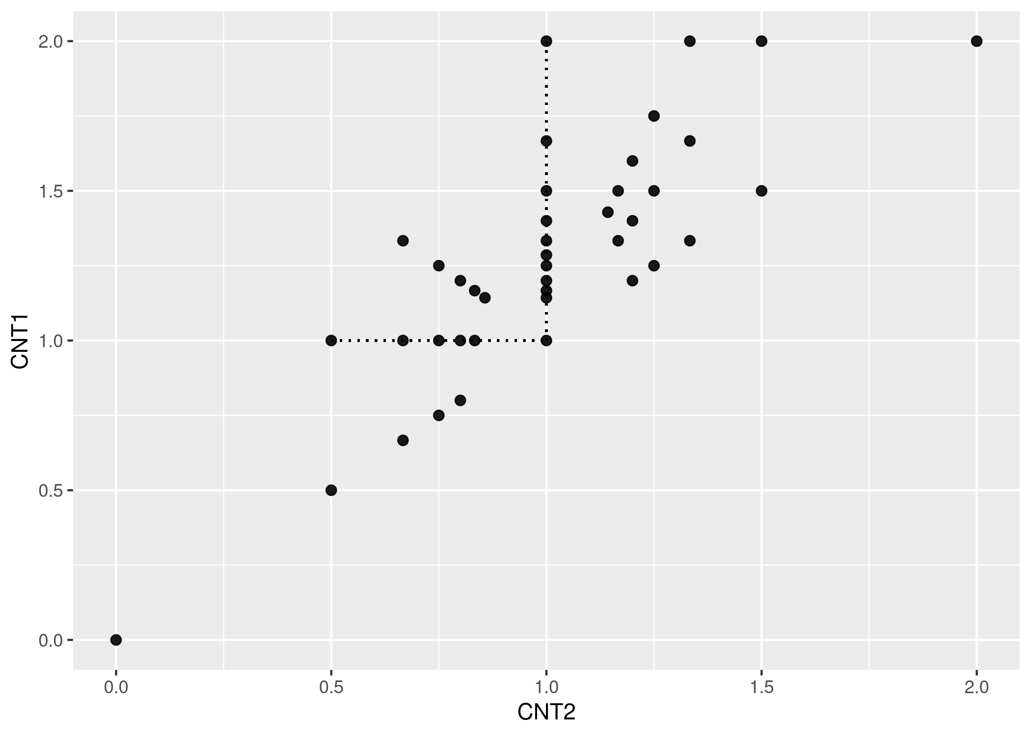
Figure 16: $\textnormal{CNT}_{1}$ vs $\textnormal{CNT}_{2}$ for system (66), with $\Pr\left[R_{j}^{i}=1\right]=1/2$ for all $i,j$ in the system. Each symbol corresponds to a specific choice of the joint distribution of $R_{1}^{5},R_{2}^{5},R_{3}^{5},R_{4}^{5}$, while keeping $R_{1}^{1}=R_{2}^{1}$, $R_{2}^{2}=R_{3}^{2}$, $R_{3}^{3}=R_{4}^{3}$, and $R_{4}^{4}=R_{1}^{4}$. Neither of $\textnormal{CNT}_{1}$ and $\textnormal{CNT}_{2}$ is a function of the other, as indicated by the horizontally and vertically aligned points.

It might be tempting to think that cyclic systems could help one in at least detecting if not measuring (non)contextuality of a system. Clearly, if a system contains a contextual cyclic subsystem, then it is contextual. This is not surprising, however, because this is true for any contextual subsystem, cyclic or not (DzhCerKuj2017, ; DzhKujFoundations2017, ). Could it be, one might wonder, that a system is always noncontextual if it does not contain a contextual cyclic subsystem? The answer is negative, as we see from the following counterexample. Let a system of dichotomous random variables be

$$\begin{array}[]{|c|c|c|c||c}\hline\cr R_{1}^{1}&R_{2}^{1}&R_{3}^{1}&&c_{1}\\ \hline\cr&R_{2}^{2}&R_{3}^{2}&R_{4}^{2}&c_{2}\\ \hline\cr R_{1}^{3}&&R_{3}^{3}&R_{4}^{3}&c_{3}\\ \hline\cr\hline\cr q_{1}&q_{2}&q_{3}&q_{4}\end{array},$$ (67)

with four contents measured in three contexts. Let the joint distributions of the three bunches be

$$\begin{array}[]{|c|c|c|c|}\hline\cr R_{1}^{1}&R_{2}^{1}&R_{3}^{1}&\\ \hline\cr-1&-1&+1&\nicefrac{{1}}{{4}}\\ \hline\cr-1&+1&-1&\nicefrac{{1}}{{4}}\\ \hline\cr+1&-1&-1&\nicefrac{{1}}{{4}}\\ \hline\cr+1&+1&+1&\nicefrac{{1}}{{4}}\\ \hline\cr\end{array},\;\begin{array}[]{|c|c|c|c|}\hline\cr R_{2}^{2}&R_{3}^{2}&R_{4}^{2}&\\ \hline\cr-1&-1&+1&\nicefrac{{1}}{{4}}\\ \hline\cr-1&+1&-1&\nicefrac{{1}}{{4}}\\ \hline\cr+1&-1&-1&\nicefrac{{1}}{{4}}\\ \hline\cr+1&+1&+1&\nicefrac{{1}}{{4}}\\ \hline\cr\end{array},\;\begin{array}[]{|c|c|c|c|}\hline\cr R_{1}^{3}&R_{3}^{3}&R_{4}^{3}&\\ \hline\cr+1&+1&-1&\nicefrac{{1}}{{4}}\\ \hline\cr+1&-1&+1&\nicefrac{{1}}{{4}}\\ \hline\cr-1&+1&+1&\nicefrac{{1}}{{4}}\\ \hline\cr-1&-1&-1&\nicefrac{{1}}{{4}}\\ \hline\cr\end{array}.$$ (68)

Here, the probabilities of the triples of values in each bunch are shown in the rightmost columns, with all remaining triples having probability zero. One can check that all random variables are distributed uniformly,

$$\Pr\left[R_{i}^{k}=-1\right]=\Pr\left[R_{i}^{k}=+1\right]=\frac{1}{2},$$ (69)

so the system is consistently connected. All pairs $\left(R_{i}^{k},R_{j}^{k}\right)$ are also uniformly distributed,

$$\begin{array}[]{|c|c|c|}\hline\cr R_{i}^{k}&R_{j}^{k}&\\ \hline\cr-1&-1&\nicefrac{{1}}{{4}}\\ \hline\cr-1&+1&\nicefrac{{1}}{{4}}\\ \hline\cr+1&-1&\nicefrac{{1}}{{4}}\\ \hline\cr+1&+1&\nicefrac{{1}}{{4}}\\ \hline\cr\end{array}.$$ (70)

This means that the system is strongly consistently connected: whenever a set of contents is measured in two contexts, their joint (here, pairwise) distributions coincide. Because the variables in each bunch are pairwise independent, any cyclic subsystem of this system is noncontextual. The entire system, however is contextual. Indeed, in the hypothetical coupling satisfying the definition of noncontextuality, if $\left(S_{1}^{1},S_{2}^{1},S_{3}^{1}\right)=\left(-1,-1,1\right)$, then $\left(S_{2}^{2},S_{3}^{2},S_{4}^{2}\right)$ can only be $\left(-1,1,-1\right)$, and $\left(S_{1}^{3},S_{3}^{3},S_{4}^{3}\right)$ can only be $\left(-1,1,1\right)$. The reason for this is that in this hypothetical coupling we should have $\left(S_{1}^{1},S_{3}^{1}\right)=\left(S_{1}^{3},S_{3}^{3}\right)$, and $\left(S_{2}^{1},S_{3}^{1}\right)=\left(S_{2}^{2},S_{3}^{2}\right)$. However it should also be true that $\left(S_{3}^{2},S_{4}^{2}\right)=\left(S_{3}^{3},S_{4}^{3}\right)$, and this is not the case in the above triples: $\left(S_{3}^{2},S_{4}^{2}\right)=\left(1,-1\right)$ while $\left(S_{3}^{3},S_{4}^{3}\right)=\left(1,1\right)$. This completes the counterexample.

To summarize, we know now that the regular way in which the noncontextuality polytope $\mathbb{P}_{\mathbf{b}}$ (or $\mathbb{E}_{\mathbf{b}}$) and the polytope of all possible couplings $\mathbb{P}$ (or $\mathbb{E}$) create pockets at the vertices of the circumscribing boxes makes $\textnormal{CNT}_{1}$ and $\textnormal{CNT}_{2}$ single-coordinate distances that are equal to each other. Both of them are proportional to the degree of violation of the generalized Bell criterion derived in Ref. (KujDzhProof2016, ), $s_{1}\left(\mathbf{e_{b}^{*}}\right)-\Delta$. We have known from Ref. (KujDzhMeasures, ), that $\textnormal{CNT}_{2}$, unlike $\textnormal{CNT}_{1}$, naturally extends to a measure of noncontextuality, $\textnormal{NCNT}_{2}$, and this can be taken as a reason for preferring $\textnormal{CNT}_{2}$ to $\textnormal{CNT}_{1}$. $\textnormal{NCNT}_{2}$ is a single-coordinate distance, and in the case of cyclic systems, the properties of the noncontextuality polytope make $\textnormal{NCNT}_{2}$ proportional, with the same proportionality coefficient as for $\textnormal{CNT}_{2}$ and $\textnormal{CNT}_{1}$, to the smaller of two quantities: the degree of compliance with the generalized Bell inequality, $\Delta-s_{1}\left(\mathbf{e_{b}^{*}}\right)$, and the distance $m\left(\mathbf{e_{b}^{*}}\right)$ of $\mathbf{e_{b}^{*}}$ from the surface of the circumscribing box $\mathbb{R}_{\mathbf{b}}$. We also know that none of these regularities extend beyond the class of cyclic systems, so the general theory of the relationship between the measures considered in this paper has much left to develop.

Appendix: Proofs of the formal statements

Proof of Lemma 9.

Verify that, for any $\Delta$, each of the $n$ points

$$\mathbf{x}_{k}=\left\{\lambda_{1},\ldots,\lambda_{k}\left(1-n+\Delta\right),\ldots,\lambda_{n}\right\},k=1,\ldots,n,$$

satisfies

$$\sum\lambda_{i}x_{i,i\oplus 1}=n-1+\lambda_{k}^{2}\left(1-n+\Delta\right)=\Delta,$$

whence so does the hyperplane passing through these points. Since $n-2\leq\Delta\leq n$, the distance $n-\Delta$ is between 0 and 2, so that the hyperplane does cut each of the edges joined at the vertex.

Proof of Lemma 10.

Two odd vertices have nonoverlapping sets of edges emanating from them, and each of the two hyperplanes cuts its own set. The only case when an axis from one set is cut at the same point as an axis from another set is when the cuts are at the ends of the emanating edges, and this means that $\Delta=n-2$.

Proof of Lemma 11.

We need to show that for any other odd vertex $V^{\prime}=\left\{\lambda^{\prime}_{i}:i=1,\ldots,n\right\}$ of $\mathbb{C}_{\mathbf{b}}$, $\sum\lambda^{\prime}x_{i,i\oplus 1}\leq\Delta_{\mathbf{x}}$. This is indeed the case because for any value $\Delta^{\prime}\geq n-2$, the hyperplane segment $\sum\lambda^{\prime}e_{i,i\oplus 1}=\Delta^{\prime}$ does not cut any of the edges emanating from vertex $V$, except, possibly, at their other ends (if $\Delta^{\prime}=n-2$). Consequently, $\sum\lambda^{\prime}x_{i,i\oplus 1}<n-2\leq\Delta<\Delta_{\mathbf{x}}$.

Proof of Lemma 13.

By induction. For $n=2$ we have to show that the even vertices $\left(1-\left|e_{1}^{1}-e_{2}^{1}\right|,1-\left|e_{1}^{2}-e_{2}^{2}\right|\right)$ and $\left(\left|e_{1}^{1}+e_{2}^{1}\right|-1,\left|e_{1}^{2}+e_{2}^{2}\right|-1\right)$ are within $\mathbb{E}_{\mathbf{b}}$. For the former vertex this means that

$$\left|\left(1-\left|e_{1}^{1}-e_{2}^{1}\right|\right)-\left(1-\left|e_{1}^{2}-e_{2}^{2}\right|\right)\right|\leq\left|e_{1}^{1}-e_{1}^{2}\right|+\left|e_{2}^{1}-e_{2}^{2}\right|.$$

Without loss of generality, let the left-hand side be $\left(1-\left|e_{1}^{1}-e_{2}^{1}\right|\right)-\left(1-\left|e_{1}^{2}-e_{2}^{2}\right|\right)$. The inequality then is equivalent to

$$\left|e_{1}^{2}-e_{2}^{2}\right|\leq\left|e_{1}^{2}-e_{1}^{1}\right|+\left|e_{1}^{1}-e_{2}^{1}\right|+\left|e_{2}^{1}-e_{2}^{2}\right|,$$

which is true by the triangle inequality. For the second even vertex we have to show that

$$\left|\left(\left|e_{1}^{1}+e_{2}^{1}\right|-1\right)-\left(\left|e_{1}^{2}+e_{2}^{2}\right|-1\right)\right|\leq\left|e_{1}^{1}-e_{1}^{2}\right|+\left|e_{2}^{1}-e_{2}^{2}\right|.$$

Again, without loss of generality, let the left-hand side be $\left(\left|e_{1}^{1}+e_{2}^{1}\right|-1\right)-\left(\left|e_{1}^{2}+e_{2}^{2}\right|-1\right)$.

(1) If $e_{1}^{1}+e_{2}^{1}\geq 0$, $e_{1}^{2}+e_{2}^{2}\geq 0$, the inequality acquires the form $\left(e_{1}^{1}-e_{1}^{2}\right)+\left(e_{2}^{1}-e_{2}^{2}\right)\leq\left|e_{1}^{1}-e_{1}^{2}\right|+\left|e_{2}^{1}-e_{2}^{2}\right|$, which is true.

(2) If $e_{1}^{1}+e_{2}^{1}<0$, $e_{1}^{2}+e_{2}^{2}<0$, the inequality acquires the form $\left(e_{1}^{2}-e_{1}^{1}\right)+\left(e_{2}^{2}-e_{2}^{1}\right)\leq\left|e_{1}^{1}-e_{1}^{2}\right|+\left|e_{2}^{1}-e_{2}^{2}\right|$, which is true.

(3) If $e_{1}^{1}+e_{2}^{1}\geq 0$, $e_{1}^{2}+e_{2}^{2}<0$, we have

$$\begin{array}[]{r}\left(e_{1}^{1}+e_{1}^{2}\right)+\left(e_{2}^{1}+e_{2}^{2}\right)=\left(e_{1}^{1}-e_{1}^{2}\right)+\left(e_{2}^{1}-e_{2}^{2}\right)+2\left(e_{1}^{2}+e_{2}^{2}\right)\\ \leq\left(e_{1}^{1}-e_{1}^{2}\right)+\left(e_{2}^{1}-e_{2}^{2}\right)\leq\left|e_{1}^{1}-e_{1}^{2}\right|+\left|e_{2}^{1}-e_{2}^{2}\right|,\end{array}$$

which is true. The fourth case is analogous.

Assume now that the statement of the theorem holds for all $2\leq k<n$. We have to show that

$$s_{1}\left(\mathbf{x}\right)\leq n-2+\delta^{\left(n\right)}$$

for any even vertex of $\mathbb{R}_{\mathbf{b}}$. Without changing the values of $s_{1}$ and any of the summands in $\delta^{\left(n\right)}$, we can put the inequality in the canonical form (Lemma 8),

$$\sum_{i=1}^{n-1}x_{i,i\oplus 1}-x_{n1}\leq n-2+\delta^{\left(n\right)}.$$

Consider two cases.

(Case 1) At least one of the coordinates $x_{i,i\oplus 1}$ ($i=1,\ldots,n-1$) is a max-coordinate. Let it be $x_{12}=1-\left|x_{1}^{1}-x_{2}^{1}\right|$. We can rewrite the inequality as

$$\begin{array}[]{r}\left(\sum_{i=2}^{n-1}x_{i,i\oplus 1}-x_{n1}\right)+1-\left|x_{1}^{1}-x_{2}^{1}\right|\leq\left(n-3+\delta^{\left(n-1\right)}\right)\\ +1+\left|x_{1}^{1}-x_{1}^{n}\right|+\left|x_{2}^{1}-x_{2}^{2}\right|-\left|x_{2}^{2}-x_{1}^{n}\right|\end{array}.$$

The value of $\sum_{i=2}^{n-1}x_{i,i\oplus 1}-x_{n1}$ is equal to the $s_{1}$ of some system of rank $n-1$, and since the vector $\left\{x_{23},\ldots,x_{n-1,n},x_{n1}\right\}$ contains an even number of min-coordinates,

$$\left(\sum_{i=2}^{n-1}x_{i,i\oplus 1}-x_{n1}\right)\leq n-3+\delta^{\left(n-1\right)}$$

holds by the induction hypothesis. At the same time, obviously,

$$1-\left|x_{1}^{1}-x_{2}^{1}\right|\leq 1+\left|x_{1}^{1}-x_{1}^{n}\right|+\left|x_{2}^{1}-x_{2}^{2}\right|-\left|x_{2}^{2}-x_{1}^{n}\right|,$$

and this establishes (*) for this case.

(Case 2) All coordinates $x_{i,i\oplus 1}$ ($i=1,\ldots,n-1$) are min-coordinates. Let us then replace two of them (which is possible since $n-1\geq 2$) with the corresponding max-coordinates — this will leave the number of the min-coordinates even. The left-hand side of (*) can only increase, but we can use the argument of the previous case to show that it is still less than the (unchanged) right-hand side of (*).

This completes the proof.

References

- (1) M. Araújo, M. T. Quintino, C. Budroni, M. T. Cunha, and A. Cabello, All noncontextuality inequalities for the n-cycle scenario, Phys. Rev. A 88, 022118 (2013).
- (2) J. V. Kujala, E. N. Dzhafarov, and J.-Å. Larsson, Necessary and sufficient conditions for extended noncontextuality in a broad class of quantum mechanical systems, Phys. Rev. Lett. 115, 150401 (2015).
- (3) A. A. Klyachko, M. A. Can, S. Binicioğlu, and A. S. Shumovsky, A simple test for hidden variables in spin-1 system, Phys. Rev. Lett. 101, 020403 (2008).
- (4) R. Lapkiewicz, P. Li, C. Schaeff, N. K. Langford, S. Ramelow, M. Wieśniak, and A. Zeilinger, Experimental non-classicality of an indivisible quantum system, Nature 474, 490 (2011).
- (5) J. Bell, On the Einstein-Podolsky-Rosen paradox, Phys. 1, 195 (1964).
- (6) J. Bell, On the problem of hidden variables in quantum mechanics, Rev. Modern Phys. 38, 447 (1966).
- (7) J. F. Clauser, M. A. Horne, A. Shimony, and R. A. Holt, Proposed experiment to test local hidden-variable theories, Phys. Rev. Lett. 23, 880 (1969).
- (8) A. Fine, Joint distributions, quantum correlations, and commuting observables, J. Math. Phys. 23, 1306 (1982).
- (9) G. Bacciagaluppi, Leggett-Garg inequalities, pilot waves and contextuality, Int. J. Quant. Found. 1, 1 (2015).
- (10) J. Kofler and C. Brukner, Condition for macroscopic realism beyond the Leggett-Garg inequalities, Phys. Rev. A 87, 052115 (2013).
- (11) A. J. Leggett and A. Garg, Quantum mechanics versus macroscopic realism: Is the flux there when nobody looks? Phys. Rev. Lett. 54, 857 (1985).
- (12) P. Suppes and M. Zanotti, When are probabilistic explanations possible? Synth. 48, 191 (1981).
- (13) E. N. Dzhafarov, R. Zhang, and J. V. Kujala, Is there contextuality in behavioral and social systems? Phil. Trans. Roy. Soc. A 374, 20150099 (2016).
- (14) Z. Wang, T. Solloway, R. M. Shiffrin, and J. R. Busemeyer, Context effects produced by question orders reveal quantum nature of human judgments, Proc. Natl. Acad. Sci. 111, 9431 (2014).
- (15) E. N. Dzhafarov, V. H. Cervantes, and J. V. Kujala, Contextuality in canonical systems of random variables, Phil. Trans. Roy. Soc. A 375, 20160389 (2017).
- (16) E. N. Dzhafarov and J. V. Kujala, Probabilistic foundations of contextuality, Fortsch. Phys. - Prog. Phys. 65, 1600040 (1-11) (2017).
- (17) J. V. Kujala and E. N. Dzhafarov, Measures of contextuality and noncontextuality, Phil. Trans. Roy. Soc. A 377, 20190149 (2019).
- (18) E. N. Dzhafarov, J. V. Kujala, and J.-Å. Larsson, Contextuality in three types of quantum-mechanical systems, Found. Phys. 45, 762 (2015).
- (19) J. V. Kujala and E. N. Dzhafarov, Proof of a conjecture on contextuality in cyclic systems with binary variables, Found. Phys. 46, 282 (2016).
- (20) M. Malinowski, C. Zhang, F. M. Leupold, J. Alonso, J. P. Home, and A. Cabello, A, Probing the limits of correlations in an indivisible quantum system, arXiv:1712.06494v2 (2018).
- (21) M. Arias, G. Canas, E. S. Gomez, J. B. Barra, G. B. Xavier, G. Lima, V. D’Ambrosio, F. Baccari, F. Sciarrino, and A. Cabello, Testing noncontextuality inequalities that are building blocks of quantum correlations, Phys. Rev. A 92, 032126 (2015)
- (22) A. Crespi, M. Bentivegna, I. Pitsios, D. Rusc, D. Poderini, G. Carvacho, V. D’Ambrosio, A. Cabello, F. Sciarrino, and R., Osellame, Single-photon quantum contextuality on a chip, ACS Photonics 4, 2807-2812. (2017).
- (23) C. Flühmann, V. Negnevitsky, M. Marinelli, and J. P. Home, Sequential modular position and momentum measurements of a trapped ion mechanical oscillator, Phys. Rev. X 8, 021001 (2018).
- (24) X. Zhan, P. Kurzyński, D. Kaszlikowski, K. Wang, Z. Bian, Y. Zhang, and P. Xue, Experimental detection of information deficit in a photonic contextuality scenario, Phys. Rev. Lett. 119, 220403 (2017).
- (25) S. Abramsky, R. S. Barbosa, and S. Mansfield, The contextual fraction as a measure of contextuality, Phys. Rev. Lett. 119, 050504 (2017).
- (26) N. Brunner, D. Cavalcanti, S. Pironio, V. Scarani, and S. Wehner, Bell nonlocality, Rev. Mod. Phys. 86, 419 (2014).
- (27) B. Amaral, M. T. Cunha, and A. Cabello, Quantum theory allows for absolute maximal contextuality, Phys. Rev. A 92, 062125 (2015).
- (28) A. Grudka, K. Horodecki, M. Horodecki, P. Horodecki, R. Horodecki, P. Joshi, W. Kłobus, and A. Wójcik, Quantifying Contextuality, Phys. Rev. Lett. 112, 120401 (2014).
- (29) M. Kleinmann, O. Gühne, J.́R. Portillo, J.-Å. Larsson, and A. Cabello, Memory cost of quantum contextuality, New J. Phys. 13, 113011 (2011).
- (30) J. Bermejo-Vega, N. Delfosse, D. E. Browne, C. Okay, and R. Raussendorf, Contextuality as a resource for models of quantum computation with qubits, Phys. Rev. Lett. 119, 120505 (2017).
- (31) M. Howard, J. Wallman, V. Veitch, and J. Emerson, Contextuality supplies the ‘magic’ for quantum computation, Nature 510, 351–355 (2014).
- (32) C. Brukner, M. Zukowski, J.-W. Pan, and A. Zeilinger, Bell’s inequalities and quantum communication complexity, Phys. Rev. Lett. 92, 127901 (2004).
- (33) As Ref. (KujDzhProof2016, ) plays an important role in the present paper (see Theorem 3 and Lemmas 7-8), we should mention that we have noticed two unfortunate typos in the introduction to that paper (in Eq. 7 and Sec. 1.4). They are corrected in the arXiv’ed version of the paper, arXiv:1503.02181, and on the authors’ websites.
- (34) H. J. H. Tuenter, Minimum L1-distance projection onto the boundary of a convex set: Simple characterization, J. Optim. Theor. Appl., 112, 441 (2002).
- (35) E. N. Dzhafarov, On joint distributions, counterfactual values, and hidden variables in understanding contextuality, Phil. Trans. Roy. Soc. A 377, 20190144 (2019).
- (36) In all our previous publications was simply . However, at any cyclic system of rank is noncontextual. This will become apparent in Sec. VII: at the noncontextuality polytope fills the entire hypercube of possible values of , and a further increase in does not change this.
- (37) E. N. Dzhafarov, Replacing nothing with something special: Contextuality-by-Default and dummy measurements, in Quantum Foundations, Probability and Information. (Springer, Berlin, 2017), pp 39-44.
- (38) B. Amaral, C. Duarte, and R. I. Oliveira, Necessary conditions for extended noncontextuality in general sets of random variables, J. Math. Phys. 59, 072202 (2018).
- (39) The rest of this paragraph and Fig. 16 are modified with respect to the published version in accordance with Erratum: Contextuality and noncontextuality measures and generalized Bell inequalities for cyclic systems [Phys. Rev. A 101, 042119 (2020)], published in Phys. Rev. A.