∎
University of Geneva,
66 Bd Carl-Vogt, 1205 Geneva, Switzerland
Tel.: +41-22-379 06 25
Fax: +41-22-379 07 44
22email: maura.brunetti@unige.ch 33institutetext: J. Kasparian 44institutetext: Institute for Environmental Sciences and Group of Applied Physics,
University of Geneva,
66 Bd Carl-Vogt, 1205 Geneva, Switzerland
55institutetext: C. Vérard 66institutetext: Section of Earth and Environmental Sciences,
University of Geneva,
13 Rue des Maraîchers, 1205 Geneva, Switzerland
Co-existing climate attractors in a coupled aquaplanet
Abstract
The first step in exploring the properties of dynamical systems like the Earth climate is to identify the different phase space regions where the trajectories asymptotically evolve, called ‘attractors’. In a given system, multiple attractors can co-exist under the effect of the same forcing. At the boundaries of their basins of attraction, small changes produce large effects. Therefore, they are key regions for understanding the system response to perturbations. Here we prove the existence of up to five attractors in a simplified climate system where the planet is entirely covered by the ocean (aquaplanet). These attractors range from a snowball to a hot state without sea ice, and their exact number depends on the details of the coupled atmosphere–ocean–sea ice configuration. We characterise each attractor by describing the associated climate feedbacks, by using the principal component analysis, and by measuring quantities borrowed from the study of dynamical systems, namely instantaneous dimension and persistence.
Keywords:
Coupled aquaplanet Attractors GCM complexity1 Introduction
The Earth climate is an out-of-equilibrium system (Gallavotti, 2006) that, under the effect of a inhomogeneous distribution of solar radiation at its boundary, evolves toward statistically stationary states (Saltzman, 1983; Lucarini et al, 2014). Even neglecting possible additional non-steady forcing (for example of anthropic origin), nonlinear interactions between the main components of the climate system, i. e. atmosphere, ocean, cryosphere, biosphere, make its study highly difficult. To address the complexity of the climate, modellers have historically developed a hierarchy of models with increasing level of comprehensiveness, ranging from energy balance models to the most realistic general circulation models (Held, 2005; Jeevanjee et al, 2017). Here we apply the MIT general circulation model (MITgcm) (Marshall et al, 1997a, b; Adcroft et al, 2004) to the numerical study of a coupled aquaplanet (Marshall et al, 2007), that is a system where the full coupling between atmosphere, ocean and sea ice is taken into account, but their motion is simplified by the absence of land, the planet being entirely covered by the ocean. In this way, even if the complexity of the system is reduced with respect to the real climate system, the main nonlinear interactions between its components are still taken into account.
Under the action of a constant external forcing and at fixed values of internal parameters, the solutions of a dynamical system are attracted toward stable regions of phase space, named attractors (Milnor, 1985). The attractor is the minimal invariant closed set that attracts an open set of initial conditions converging toward as time tends to infinity. The largest such is called basin of attraction (Strogatz, 1994, p. 324). Finding the attractors and their basin of attraction is the first step in the analysis of the unperturbed dynamics. At the basin boundaries, also denoted as unstable manifolds or edge/melancholia states (Lucarini and Bódai, 2017), the dynamics is highly nonlinear, small perturbations giving rise to abrupt and potentially irreversible changes that correspond to the passage from an attractor to the other. Such endogenous crises are generally called ‘tipping points’ in climate dynamics or ‘critical transitions’ in statistical physics. Examples of tipping elements in the present-day climate are the shut-down of the overturning circulation in the Atlantic ocean, the methane release from the melting of the permafrost or the dieback of the Amazon forest (Lenton et al, 2008).
Thus the attractors characterisation helps in predicting the system response to perturbations. A huge effort is presently under way to understand properties of attractors and tipping points (Bathiany et al, 2016), to develop early warning systems for detecting the approach to such thresholds (Dakos et al, 2008) and to clarify the nature of perturbations (internal variability and self-reinforcing feedbacks) or external forcing (for example of astronomical or anthropic origin) that could give rise to critical transitions (Rose et al, 2013). A treatment of noise-induced transitions is given in Lucarini and Bódai (2019).
Here we systematically search for attractors in an aquaplanet, that is the simplest configuration in coupled atmosphere-ocean-sea ice models. We show how the large-scale structure of the unperturbed system changes when we improve the physical description of the MITgcm used to run the simulations. Namely, we compare the more accurate model set-up where dissipated kinetic energy is re-injected within the system as thermal energy, and the bulk cloud albedo varies with latitude (setUp1), with the one where dissipated kinetic energy is lost and bulk cloud albedo is constant (setUp2). While previous studies identified two (Budyko, 1969; Sellers, 1969; Ghil, 1976; Lucarini et al, 2010; Abbot et al, 2011; Boschi et al, 2013), three (Ferreira et al, 2011; Lucarini and Bódai, 2017), or four co-existing attractors (Rose, 2015), we obtain up to five attractors that co-exist under the same external forcing, represented in our simulations by fixed values of solar irradiation and atmospheric CO2 content. This demonstrates that a simplified system such as a coupled aquaplanet is sufficiently rich to produce a complex dynamical structure.
Each attractor is associated to a different climate, ranging from snowball conditions (Kirschvink, 1992) to a hot state where the sea ice completely disappears. We characterise each climate by describing ocean overturning circulation, heat transport, cloud cover and surface air temperature distribution, and by estimating a list of averaged global quantities and energy budget components to reveal the dominant nonlinear feedbacks at play in each attractor. We take advantage of some powerful tools borrowed from the theory of dynamical systems and statistics (Saltzman, 1983), such as instantaneous dimension and persistence (Lucarini et al, 2016; Faranda et al, 2017b, a), and principal component analysis, to further explore the dynamics of the attractors and differentiate them.
The paper is organised as follows: in Section 2 we present the MITgcm configurations and the techniques for testing the complexity of time series, in Section 3 we describe the results of simulations, and finally in Section 4 we discuss the results in the light of previous findings and we suggest further developments.
2 Methods
2.1 MITgcm
We use the MIT general circulation model (MITgcm, version c65q) (Marshall et al, 1997a, b; Adcroft et al, 2004) to simulate a coupled aquaplanet, i.e. a planet homogeneously covered by a 3000 m deep ocean. It offers a simpler system than the actual Earth configuration, as no continents perturb the ocean currents and the atmosphere circulation.
The MITgcm is a coupled atmosphere-ocean-sea ice model, where the same kernel is employed for representing atmosphere and ocean dynamics (Marshall et al, 2004) on a common cubed-sphere grid. The physics packages activated for the oceanic component are the Gent and McWilliams scheme (Gent and McWilliams, 1990), used to parameterise mesoscale eddies, and the KPP scheme (Large and Yeager, 2004) for accounting of vertical mixing processes in the ocean surface boundary layer and the interior. The thermodynamic properties of sea ice are implemented through the Winton model (Winton, 2000), while sea ice dynamics is neglected. Concerning the atmospheric component, the physics module called 5-layer SPEEDY (Molteni, 2003) comprises a four-band radiation scheme, boundary layer and moist convection schemes, resolved baroclinic eddies and diagnostic clouds. Orbital forcing is prescribed at present-day values and the atmospheric content is fixed to a constant value of 326 parts per million.
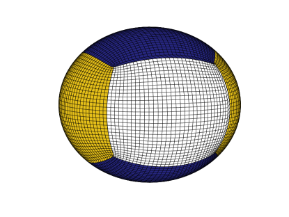
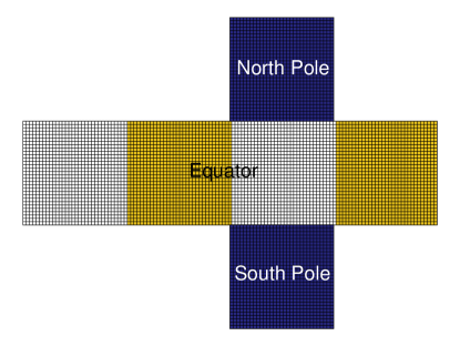
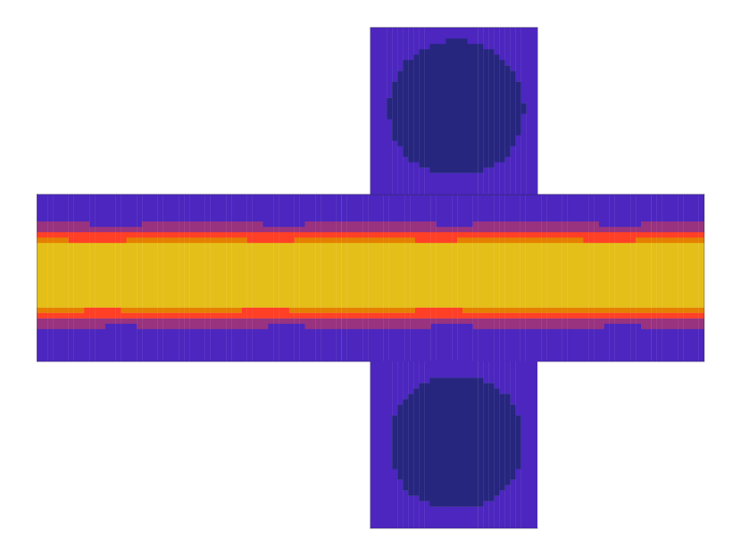
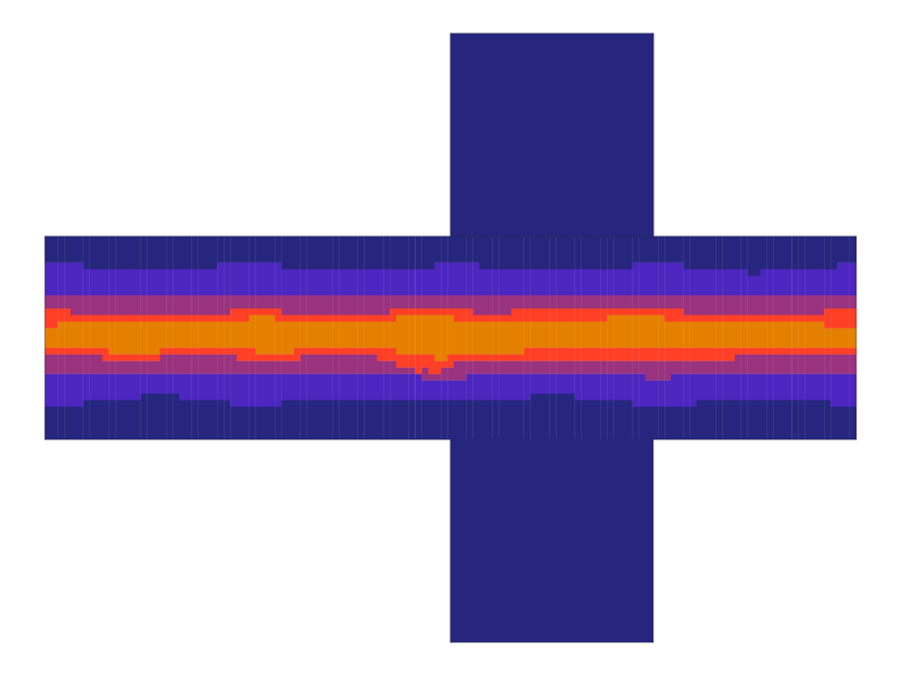
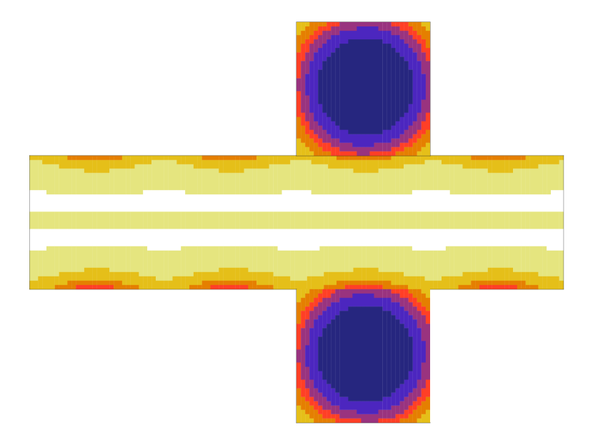
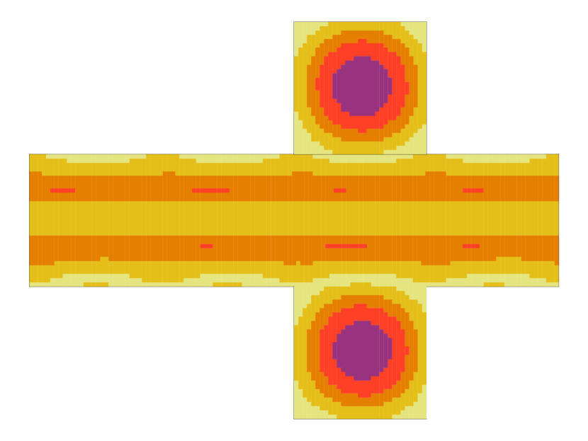
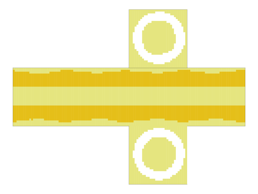
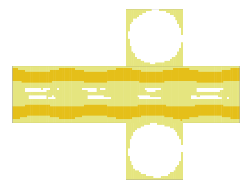
We consider a low resolution cubed-sphere (CS) grid (Fig. 1), where each face of the cube has 32 32 cells (CS32), giving a horizontal resolution of 2.8∘. The ocean grid has 15 vertical levels with different thickness, from 50 m near the surface to 690 m in the abyss, for a total depth of km. In this way, simulations over thousands years can be run in a reasonable amount of CPU time (namely, 100 yr in 1 day on a typical workstation).
Two different configurations are considered. In the first, more comprehensive set-up, denoted as setUp1, the bulk cloud albedo varies with latitude, like in version 40 of SPEEDY (Kucharski et al, 2006, 2013), where this modification has been implemented in order to correct a too strong high-latitude solar radiation flux. Furthermore, dissipated kinetic energy is re-injected within the system as thermal energy, allowing for an improved budget at Top-Of-Atmosphere (TOA) (Lucarini and Ragone, 2011; Lucarini and Pascale, 2014). This configuration is the same as that used for Run4 in Brunetti and Vérard (2018). In the second set-up, called setUp2, the bulk cloud albedo is constant, as implemented in the 5-layer SPEEDY (Molteni, 2003) and friction energy is lost, like in the configuration used for Run3 in Brunetti and Vérard (2018).
The values of input numerical parameters, such as vertical diffusivity within the ocean and snow/ice/ocean albedos, are the same as those used in Brunetti and Vérard (2018) and are listed in Table 1. Their choice minimises the drift in the global ocean temperature, and are within the observed range reported, for example, in Nguyen et al (2011). Afterwards, following the tuning procedure used by other groups (Gent et al, 2011; Tang et al, 2016), only the relative humidity threshold for low clouds (a parameter referred as in MITgcm atmospheric module) has been adjusted in such a way that, starting from an initial condition with average ocean temperature of 8.9∘C, the simulation ends up to a warm state. Then, all the simulations within a given set-up have been performed using the same value of , denoted by (namely, for setUp1 and for setUp2).
| Ocean albedo | 0.07 |
| Bulk cloud albedo | 0.38 |
| Max sea ice albedo | 0.64 |
| Min sea ice albedo | 0.20 |
| Cold snow albedo | 0.85 |
| Warm snow albedo | 0.70 |
| Old snow albedo | 0.53 |
| Vertical diffusivity [m2/s] | |
| Horizontal diffusivity [m2/s] | 0 |
2.2 Complexity assessment of time series
When a dynamical system is multistable, the solutions for a given value of internal parameters can be attracted to different regions in phase space, called attractors. The properties of such regions can be reconstructed from the time series of given observables. Several techniques exist for testing the complexity of time series (Tang et al, 2015). Here we consider two methods. The first is derived from nonlinear dynamics to describe attractor properties in phase space, namely instantaneous dimension and persistence (Lucarini et al, 2016; Faranda et al, 2017b, a). The second, the principal component analysis, is used in statistical studies and provides information on the spatial modes of variability of the climate dynamics on each attractor. We apply these techniques to the yearly averaged SAT series, at each horizontal grid point, after the transients die out and the state is stabilised on a given attractor. For each attractor, the length of the time series is at least 1500 yr.
2.2.1 Instantaneous dimension and persistence of trajectories
The mean dimension of the attractor is the number of degree of freedom sufficient to describe the dynamics when the system has settled down into the attractor. Considering the large number of degree of freedom, the so called embedding method (Grassberger and Procaccia, 1983) cannot be used. Rather, we rely on a more robust approach that allows to estimate the distribution of instantaneous dimensions of the attractor (Lucarini et al, 2016; Faranda et al, 2017b, a). The idea is to count the number of times a trajectory in phase space returns within a sphere centered on an arbitrary point on the attractor. Taking the logarithm of the distance between and all the other observations , and defining
| (1) |
the problem of finding the number of returns within the small sphere becomes equivalent to find the probability of exceeding a certain threshold associated to the quantile of the series . The theorem presented in Freitas et al (2010) and modified by Lucarini et al (2012) guarantees that in the case of large number of degrees of freedom such probability is the exponential member of the generalised Pareto distribution:
| (2) |
where is the location parameter and is the scale parameter, both depending on the chosen point . Interestingly, provides the dimension around , . The average over a sufficiently large sample of points gives the attractor dimension, . We have checked the stability of the results against changes in the quantile within the range , and we have used the Anderson-Darling test for testing the hypothesis that the extreme values of the distribution follow a generalised Pareto distribution.
One can further develop the analysis of the attractor by considering the extremal index , a parameter that measures the degree of clustering of extreme values in a stationary process (Smith and Weissman, 1994; Moloney et al, 2019). The extremal index can take values in the interval . It has been shown that it is related to the reciprocal of the mean cluster size of exceedances over a high threshold (Leadbetter, 1983), or equivalently to the reciprocal of the averaged residence time of trajectories in the vicinity of (Faranda et al, 2017b, a): low (respectively high) values of correspond to long (short) persistence of trajectories near . The value of is obtained through the estimator defined in Ferro and Segers (2003).
2.2.2 Principal component analysis
We sought for spatial modes in the dynamics of each attractor, by performing a principal component analysis (PCA) on the temporal series of yearly averaged SAT after the system was stabilised. The PCA was performed with Matlab’s function pca. The temporal series at each point are projected on the successive principal components. Their mapping defines spatial modes displaying regions that are spatially correlated, anti-correlated or independent at inter-decadal time scale.
3 Results
3.1 Characterisation of the climate in each attractor
Under the same forcing, represented by a mean annual incoming solar radiation at the top of the Earth’s atmosphere of 1368 W m-2 and a fixed level of atmospheric CO2 of 326 parts per million, the ensemble of considered initial conditions relaxes to different final statistically stationary states, i.e. attractors in the phase space. We have obtained five different attractors, respectively denoted as hot state, warm state, cold state, waterbelt and snowball in setUp2 and four attractors (the same as before except the hot one) in setUp1. This is remarkable because, to our knowledge, three (hot111The hot state is called ‘warm’ in Ferreira et al (2011); Rose (2015). We prefer to call ‘hot’ the attractor without ice cover and ‘warm’ the temperate state that is also obtained in energy balance models., cold state and snowball in Ferreira et al (2011)) and four attractors (the previous ones plus the waterbelt in Rose (2015)) had been obtained to date using MITgcm with lower resolution222The attractors in Ferreira et al (2011); Rose (2015) are obtained using CS24 ( cells per cube face), slightly different ice/snow albedos with respect to the ones used here and listed in Table 1, and a solar constant of W/m2. Vertical diffusivity and CO2 content are the same as here. Ocean and bulk cloud albedos, the parameter and the type of cloud albedo parameterisation are not specified nor if thermal energy has been re-inserted within the system. Ice thickness diffusion is included to mimic ice dynamics. We have verified that the waterbelt can be obtained in CS24 without ice thickness diffusion, while preliminary results show that the warm state is not stable in CS24 with the considered parameters., and only two (Budyko, 1969; Sellers, 1969; Ghil, 1976; Abbot et al, 2011; Lucarini et al, 2010; Boschi et al, 2013) or three attractors (Rose and Marshall, 2009; Lucarini and Bódai, 2017) using energy balance models or intermediate complexity models.
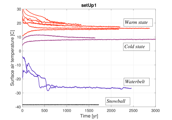
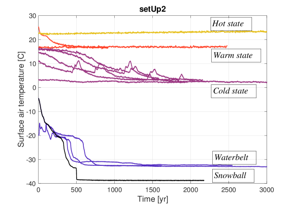
The initial conditions (ICs) are constructed in two ways. In the first, the ocean is initialised from a state of rest, without sea ice and with a homogeneous salinity at 35 psu; we take a zonal mean temperature given by , where is the number of vertical levels, is the vertical index, , and is the latitude; this IC has an average ocean temperature of 8.9∘C and is denoted by IC8.9; we homogeneously change the ocean temperature distribution by varying its mean value. In the second, we run simulations with different values of the parameter, so to obtain extremely cold or warm conditions starting from the same IC8.9; we thus use the final pickup files as ICs, this time with the value of that is used for all the simulations within a given set-up (see Section 2.1). These two methods allow us to construct an ensemble of different ICs that span initial global averages of surface air temperature (SAT) ranging from -40∘C to 35∘C.
Fig. 2 shows the time evolution of SAT and how different initial conditions converge toward the attractors. Note that not only the number, but also the position of the attractors depends on the considered set-up. In order to obtain the snowball state, where ice entirely covers the planet, and the waterbelt, where there is an equatorial oasis of open water, we have varied the maximal allowed thickness of sea ice in the range m (not all the attempts are shown in Fig. 2). Among all, only one single IC converged to the snowball attractor in setUp2, namely the one with m, all the others being attracted by the waterbelt state. This means that obtaining a snowball starting from non-snowball ICs is unlikely in the considered set-ups of MITgcm. Moreover, the dependence on may be a spurious effect of the absence of sea ice dynamics in our simulations. The waterbelt (Pierrehumbert et al, 2011)333Also called ‘slushball’, ‘soft’ snowball or Jormungand state (Abbot et al, 2011), depending on the mechanism that determines such state. and the snowball had already been shown to strongly depend on ocean (Poulsen et al, 2001) and sea ice dynamics (Lewis et al, 2007; Voigt and Abbot, 2012), sea ice/snow albedo parameterisations, cloud radiative forcing and ocean/atmosphere heat transports (Yang et al, 2012). In particular, we confirm that is harder to enter into the snowball state when sea ice dynamics is excluded as in our simulations (Lewis et al, 2007; Voigt and Abbot, 2012; Rose, 2015).
Some of the ICs ending up to the cold state in setUp2 (see Fig. 2, right panel, purple curves) show fast and transient increases in SAT. We have verified that such abrupt changes are related to the sudden reduction of sea ice in small parts of the polar regions, the SAT responding through the ice-albedo feedback on a short timescale of the order of some decades. Such abrupt changes are coupled to variations in salinity, as also discussed by Rose et al (2013) where they were shown to be related to the abrupt loss of salt stratification in the polar ocean. However, this internal variability is not sufficient to attract the solution to the warm state, and the solution finally evolves toward the cold attractor.
In Table 2 global mean values of SAT, ocean temperature, sea ice extent and corresponding latitude of sea ice boundary, calculated from the last 100 yr of simulations, are listed in order to illustrate their dependence on the chosen set-up (setUp1 in black, setUp2 in gray). The two main indicators of simulation quality discussed in Brunetti and Vérard (2018), namely the energy imbalance at Top-Of-Atmosphere (TOA) and at the ocean surface, are also listed in Table 2.
The former is an indicator of the limitations existing within a given climate model, at the level of both numerical implementation and physical parameterisations (Lucarini and Ragone, 2011; Lucarini and Pascale, 2014; Lembo et al, 2019). In our case it is in general larger in setUp2 than in setUp1, confirming that the latter configuration is more accurate than the former, since it properly includes friction heating444We have verified that the TOA imbalance does not depend on the considered cloud albedo parameterisation.. Note that the values of TOA imbalance in setUp2 are of the same order of magnitude of some IPCC climate models in the preindustrial scenario (see Fig. 2 in Lucarini and Ragone (2011)).
The ocean surface imbalance of radiation flux is related to the ocean temperature drift, , through (where kg m-3 is the sea water density, J(K kg)-1 is the specific heat capacity, and m is the ocean depth). We have verified that all our simulations have at the equilibrium. From the values in Table 2, it can be seen that in all the simulations the imbalance is indeed much smaller than the standard deviation.
| Attractor | Snowball | Waterbelt | Cold state | Warm state | Hot state |
| SAT [∘C] | — | ||||
| Ocean temperature [∘C] | — | ||||
| Sea ice extent [ km2] | 509.9 | — | |||
| 509.9 | 0 | ||||
| Latitude of sea ice boundary | 0 | 16 | 49 | 57 | — |
| 0 | 9 | 43 | 60 | 90 | |
| TOA budget [] | — | ||||
| Ocean surface budget | — | ||||
| [] |
Each attractor corresponds to a qualitatively different climate, which is the result of the competition among several nonlinear mechanisms and interactions between ocean, atmosphere and sea ice. Among them, the main feedbacks influencing the climate system include: (i) the positive ice-albedo feedback (ice is more reflective than water surfaces: the more incoming radiation, the more the ice melts, the more the surface warms); (ii) the negative Boltzmann radiative feedback (warmer surface emits more radiation back to space); (iii) the cloud feedback (more clouds reflect more short-wave radiation back to space, and at the same time more long-wave radiation back to the surface).
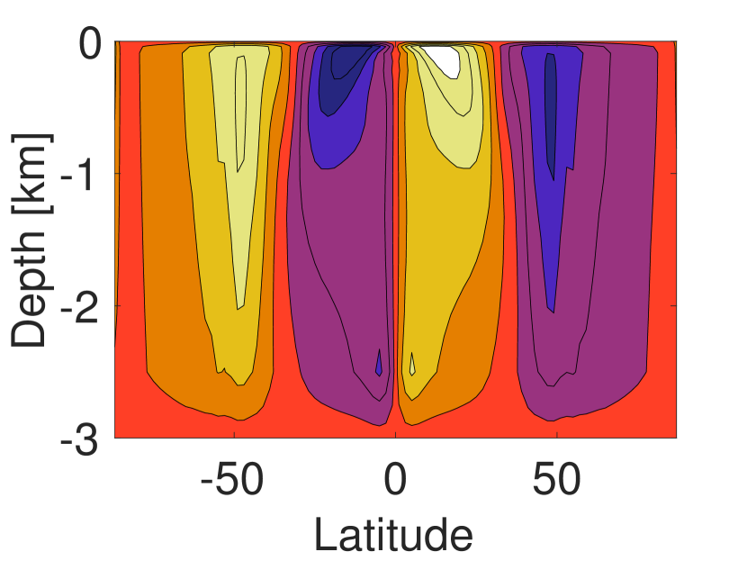
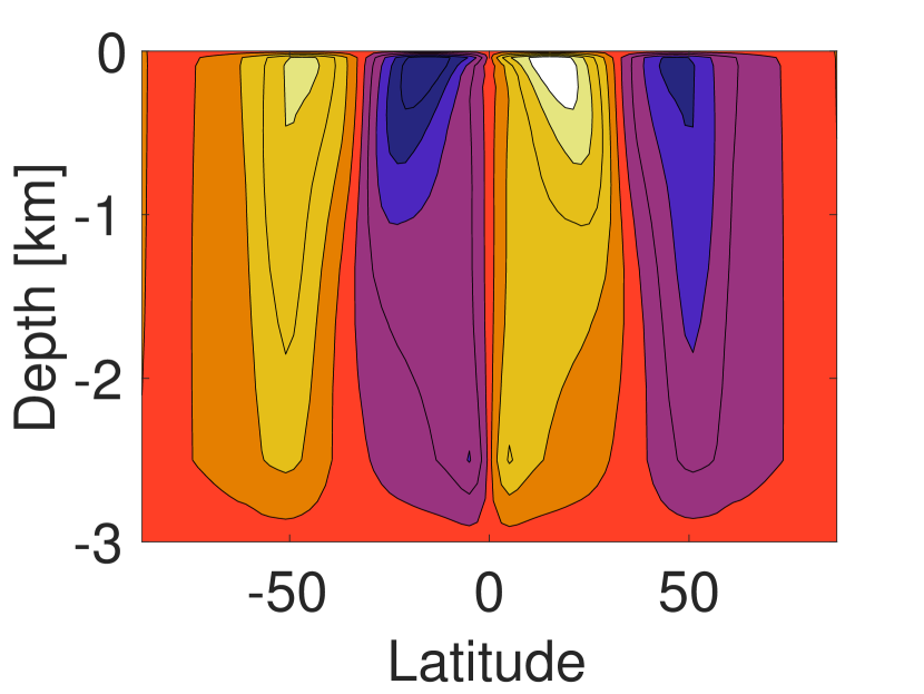
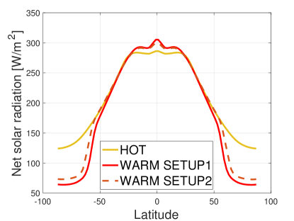
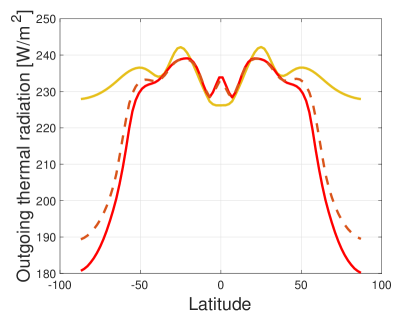
We compare the distribution of SAT (Figs. 3-4, first column), cloud fraction (second column), ocean overturning circulation (third column), heat transport and sea ice extent (fourth column) for each attractor in setUp1 (Fig. 3) and in setUp2 (Fig. 4). The components of the radiation budget at TOA, in the atmosphere and at the surface are listed in Table 3. In the snowball, where ice completely covers the ocean surface, the ice-albedo feedback dominates, since clouds are practically absent at all latitudes, the effective transmissivity of the atmosphere in the long-wave spectrum being very close to one, (see Table 3)555Note that the transmissivity is defined as the ratio between outgoing thermal radiation at TOA and upward thermal radiation at surface, see Table 3, and it is governed by the cloud feedback as well as clear-sky processes.. In the waterbelt, the sea ice boundary is found at latitudes of 16∘ in setUp1 (9∘ in setUp2), the free ocean surface absorbs more energy due to its lower albedo, and clouds form above the warmer equatorial region. In agreement with Rose (2015), the waterbelt implies that the ocean circulation is sufficiently organised so that heat can be emitted over a restricted range of latitudes where the ice is absent. Thus the waterbelt can be viewed as the result of the competition between the destabilising ice-albedo feedback over the ice-covered surface and the stabilising effects of the ocean circulation over the ice-free surface. In the cold state, where ice boundary reaches latitudes of in setUp1 (43∘ in setUp2), clouds start to play a more relevant role, also in the polar regions, the trasmissivity reaching an average value of (see Table 3). In the warm state, clouds are almost homogeneously distributed over all latitudes, and the competition is essentially between the Boltzmann and the cloud feedbacks, the transmissivity being , lower than the present-day transmissivity that is of the order of 0.6 (Wild et al, 2013). Finally, in the hot state cloud cover is high everywhere and the transmissivity reaches a very low value of , meaning that within this hot climate a large fraction of long-wave radiation remains trapped at the surface in particular because of the presence of clouds.
SAT [∘C] Cloud cover % Overturning circ. [Sv] Heat transport [PW]

Snowball
Waterbelt
Cold state
Warm state


SAT [∘C] Cloud cover % Overturning circ. [Sv] Heat transport [PW]


Snowball
Waterbelt
Cold state
Warm state
Hot state


| Attractor | Snowball | Waterbelt | Cold state | Warm state | Hot state |
|---|---|---|---|---|---|
| Solar radiation | |||||
| Reflected at TOA | 184.3 | 163.8 | 117.1 | 114.3 | — |
| 183.9 | 171.9 | 117.7 | 109.8 | 105.3 | |
| Absorbed by atmosphere | 112.0 | 110.5 | 101.5 | 97.2 | — |
| 112.3 | 112.2 | 104.8 | 95.3 | 86.9 | |
| Absorbed by surface | 45.7 | 67.7 | 123.4 | 130.5 | — |
| 45.8 | 57.9 | 119.5 | 136.9 | 149.8 | |
| Reflected at surface | 70.7 | 63.9 | 36.6 | 26.3 | — |
| 71.0 | 68.0 | 44.4 | 23.9 | 11.3 | |
| Thermal radiation | |||||
| Outgoing at TOA | 158.2 | 179.3 | 225.2 | 228.0 | — |
| 157.8 | 168.5 | 221.3 | 229.6 | 234.4 | |
| Up surface | 171.9 | 209.2 | 356.1 | 397.5 | — |
| 171.2 | 186.2 | 326.2 | 402.0 | 438.6 | |
| Down surface | 87.2 | 134.4 | 307.6 | 352.3 | — |
| 86.5 | 106.1 | 273.8 | 354.6 | 392.2 | |
| 0.92 | 0.86 | 0.63 | 0.57 | — | |
| 0.92 | 0.90 | 0.68 | 0.57 | 0.53 | |
| Sensible heat | 17.7 | 17.5 | 15.3 | 11.1 | — |
| 18.1 | 18.0 | 18.6 | 12.3 | 9.3 | |
| Latent heat | 14.0 | 39.3 | 96.2 | 100.5 | — |
| 14.0 | 27.8 | 92.9 | 101.1 | 105.4 |
![[Uncaptioned image]](/html/1907.03255/assets/x47.png)
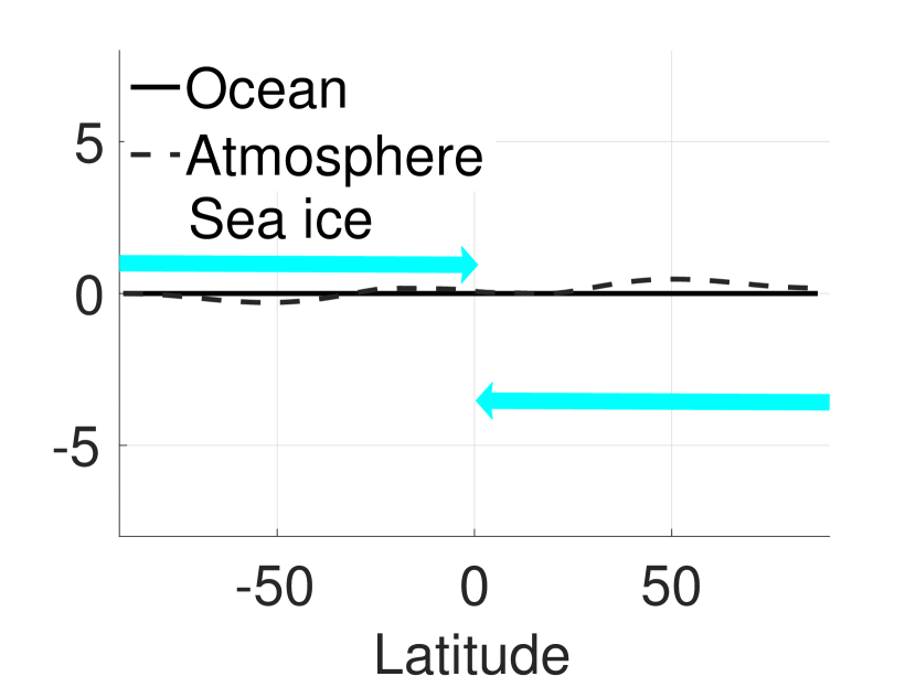
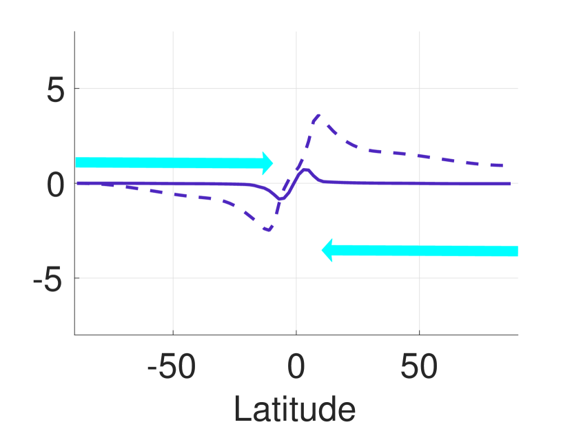
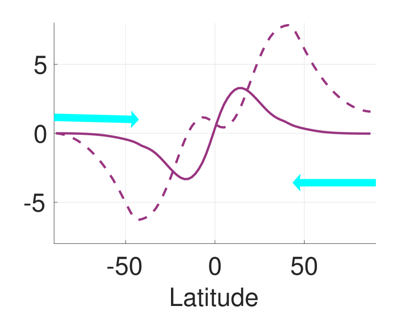
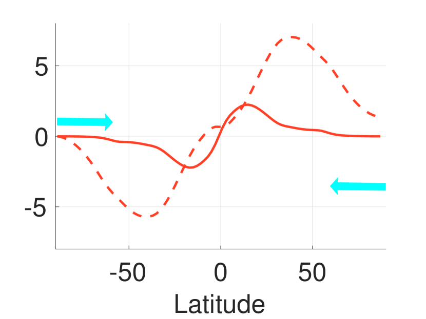
The ocean overturning circulation, shown in the third column of Figs. 3-4, is overall very weak in the snowball, except near the Equator, where a series of small and extremely intense cells develop. Since these cells are disconnected in latitude, the associated meridional heat transport turns out to be very weak (see first panel along the fourth column in Figs. 3-4). As the global SAT increases, the circulation within the ocean is organised in larger overturning cells, anti-symmetrical with respect to the Equator. Positive values correspond to clockwise circulation in Sv (1 Sv m3 s-1). Even if these overturning cells are still quite irregular in the waterbelt (much less in setUp1 than in setUp2), the ocean circulation turns out to be responsable of heat transport over a restricted range of latitudes where the ice is absent (see last column in Figs. 3-4), in qualitative agreement with Rose (2015). The overturning cells reach high intensity and extent in cold and warm states. In particular, the polar cells become slightly deeper and stronger in the cold state than in the warm one. In the hot state that occurs in setUp2, additional overturning cells can develop in the polar regions as they become ice-free (see last panel in the third column of Fig. 4).
The poleward heat transport is proportional to the strength of the circulation multiplied by the temperature gradient at the concerned latitudes, and it is dominated by the surface circulation (Boccaletti et al, 2005). Thus we see from the panels in the fourth column of Figs. 3-4 that the ocean heat transport is negligible in the snowball, where the overturning cells have small meridional extent and temperatures are quite homogeneous, while it reaches several petawatts (PW) when the surface circulation is well organised through the appearance of overturning cells that connect latitudes with large meridional temperature gradient. In particular, we observe that the peak of the ocean heat transport is of 3 PW in the cold state, larger than the corresponding value in the warm state. This can be explained by the larger meridional temperature gradient in the cold state, the intensity of the overturning cells in the tropical regions being very similar in the two attractors. The robust feature observed in Ferreira et al (2011) for the existence of the cold state, namely a meridional structure of the ocean heat transport with a shoulder at mid-latitudes, is also present in our cold attractor, as can be seen from the behaviour of the ocean heat transport near the sea ice boundary (see Figs. 3-4, fourth column, arrow and solid line in the panel corresponding to the cold state). In the warm state, such shoulder appears at higher latitudes, while in the hot state in setUp2 it disappears and heat can reach the North/South pole with a complete melting of sea ice.
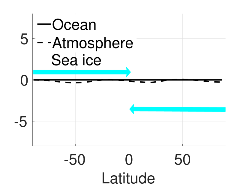
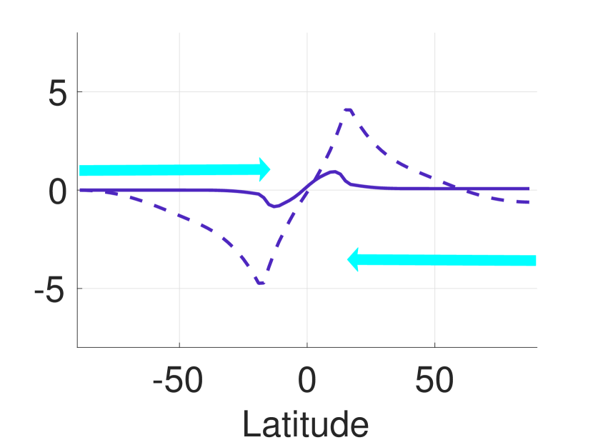
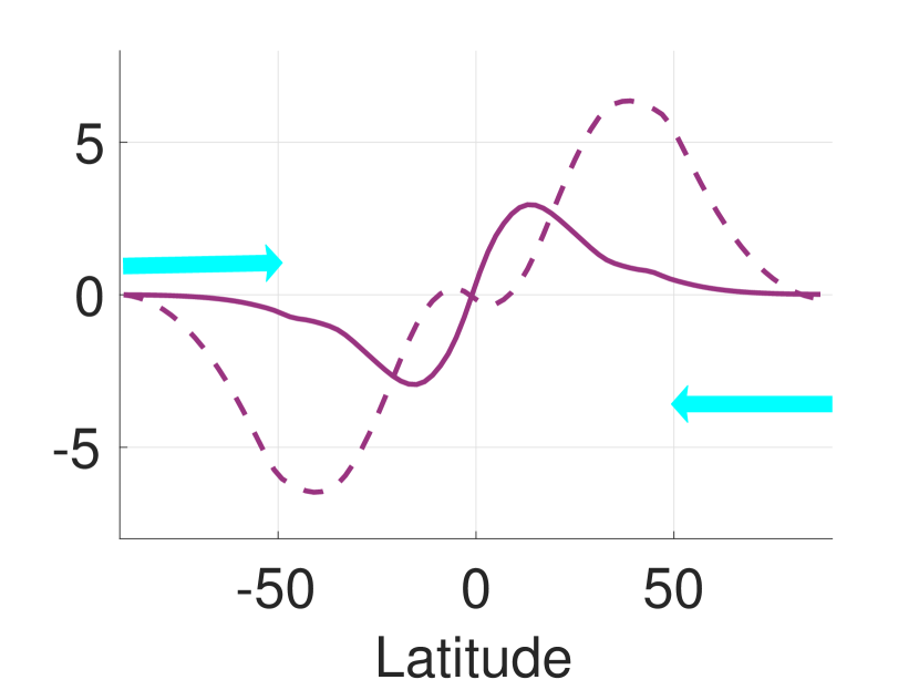
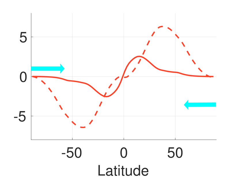
We have verified that the hot state is still present if we turn on the re-injection of dissipated kinetic energy, while keeping the cloud albedo constant in latitude. This shows that the appearance of the hot state depends on the cloud albedo parameterisation, in particular on cloud reflection properties (Donohoe and Battisti, 2012) and on the amount of solar radiation that is allowed to enter at high latitudes. In Fig. 5 the net solar radiation and the outgoing long-wave radiation at TOA are shown as a function of latitude for warm and hot states in both set-ups. We can see that the radiation at TOA for the hot state agrees with the one shown in Ferreira et al (2011). The zonal averages of both TOA thermal and solar radiation for the warm state differ at high latitudes in the two set-ups, showing that the main difference between the two considered parameterisations of cloud albedo occurs in the polar regions. We cannot exclude however that changing the solar constant or CO2 content would allow for the presence of the hot state also in setUp1.
We note that the atmospheric heat transport is very similar in cold, warm and hot states. Therefore, it does not play a relevant role in distinguishing between these attractors (see Figs. 3-4, fourth column, dashed line), in agreement with Caballero and Langen (2005); Boschi et al (2013) where it is shown that for sufficiently large mean global temperature and small meridional gradient the atmospheric heat transport stays constant. Values of atmospheric heat transport not returning to zero in the north polar region are the signature of a remaining energy imbalance at TOA, which we have not corrected to display the limitations within the considered set-up of the numerical model (Brunetti and Vérard, 2018). The TOA imbalance is larger in setUp2 than in setUp1 (compare also values in Table 2), confirming that the former is indeed a less accurate configuration for MITgcm.
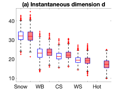
3.2 Complexity assessment of time series
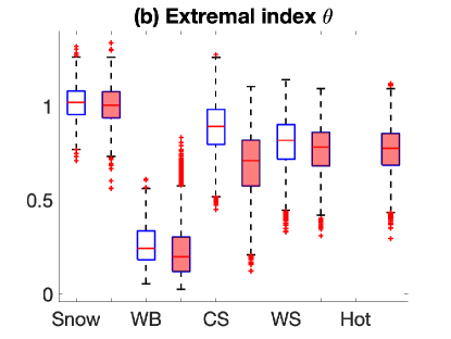
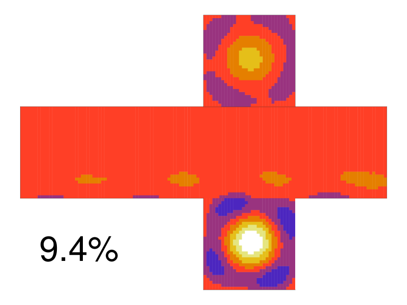
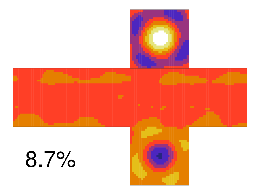
The attractors can be characterised by quantities widely used in the study of dynamical systems, namely the instantaneous dimension and the persistence (Lucarini et al, 2016; Faranda et al, 2017b, a). These quantities have been calculated from yearly averaged SAT time series, i. e., for each point on the horizontal cubed-sphere grid (see Fig. 1). The time series length is at least 1500 yr for each attractor. In Fig. 6-, we show the resulting box plots for all the attractors and both set-ups. The instantaneous dimension , that represents the minimal number of degrees of freedom able to describe the system, decreases from a value around 32 in both set-ups for the snowball, to a value around 18 for the hot state (Fig. 6). The extremal index is related to the inverse of trajectories persistence: low (respectively high) values of correspond to long (short) persistence of trajectories near a given point on the attractor. is in general near 0.8 in all the attractors, except in waterbelt where it is of the order of 0.2, and in snowball where it is close to 1 (see Fig. 6).
In order to understand the meaning of these dynamical measures, it is helpful to remember what happens in the Lorenz system (Lorenz, 1963). In such prototypical system the maxima of the instantaneous dimensions are found between the two wings, where the trajectories diverge the most and the instability is stronger (see Faranda et al (2017b) and Fig. A.1 in the Supplementary Information of that paper). The fact that stronger instabilities are associated to higher instantaneous dimensions is also supported by Schubert and Lucarini (2016); Faranda et al (2017a, b) where it is shown that higher meridional temperature gradients, associated to blocking events, give rise to higher values of Liapunov exponents and of instantaneous dimension, respectively.
The waterbelt state is characterised by strong meridional gradients localised at the ice edges, as can be seen in Figs. 3-4. This can explain the higher instantaneous dimension of this attractor with respect to the cold, warm and hot ones. On the contrary, since the snowball SAT is very uniform, as can be seen from Figs. 3-4, one would expect a low value of the instantaneous dimension. However, the fact that the extremal index is close to 1 in snowball means that clustering of exceedances is not occurring in snowball time series and that we are measuring irrelevant dynamical features that correspond to independently and identically distributed random fluctuations (Moloney et al, 2019) giving a high value of the instantaneous dimension. It is important to recall that the value of the dynamical estimator does not correspond to the true dimensionality of the system, since the convergence is very low, as discussed for example in Gálfi et al (2017). Rather, such estimators give useful informations when compared between each other in different attractors and provide an efficient way to obtain information on time series behavior.
The fact that the instantaneous dimension decreases from the waterbelt to the hot state, that is from a state with strong meridional temperature gradient to one where temperature distribution becomes more homogeneous, is in agreement with Shao (2017), based on the sample entropy method, and Lucarini and Bódai (2017); Faranda et al (2019) where it is shown that strong and localised temperature gradients are associated to low predictability.
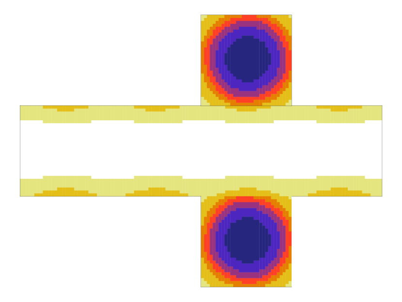
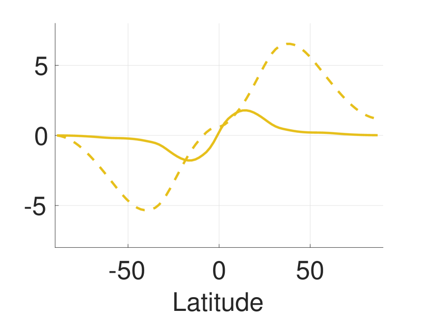
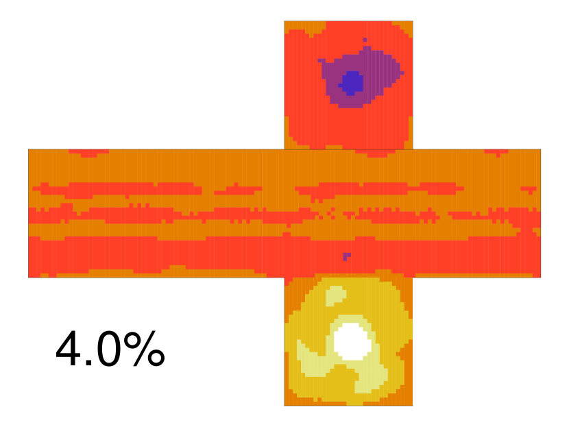
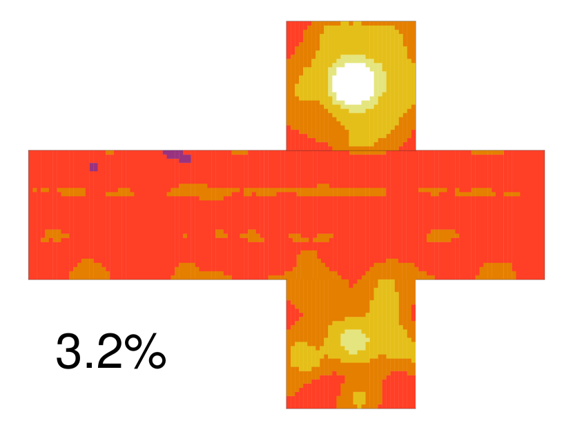
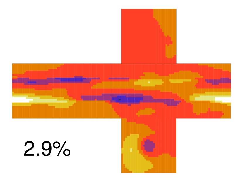
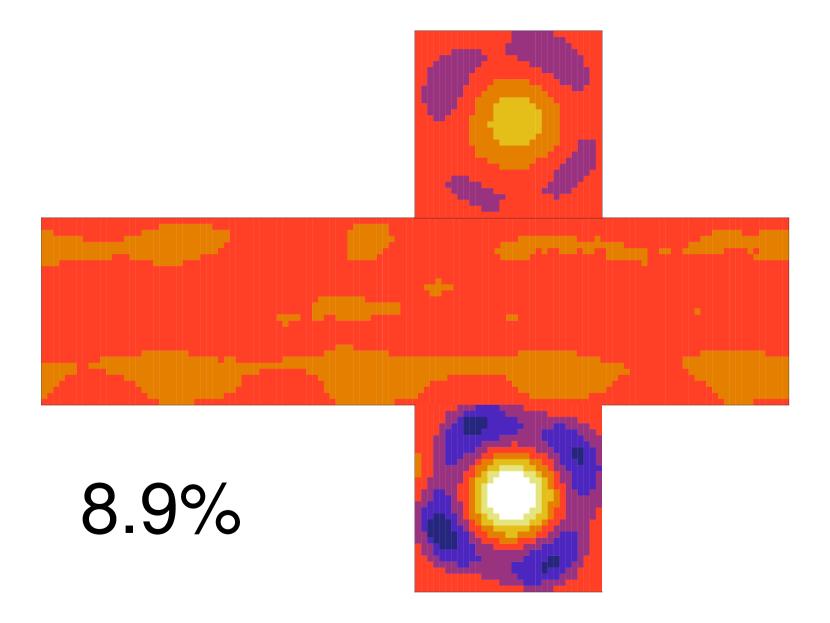
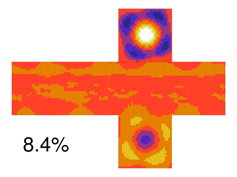
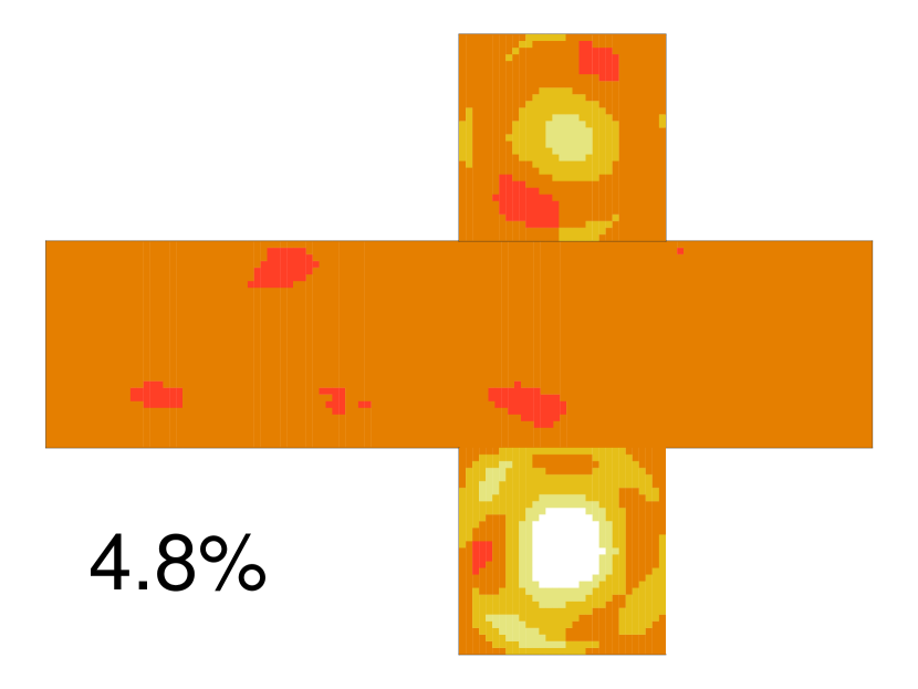
Finally, a principal component analysis evidenced the spatial structure of each attractor, providing hints about the main feedbacks at play in each of them. In particular, the principal components (PCs), or modes, assess the spatial regions where most of the variability takes place in each attractor and whether this variability is correlated between different regions.
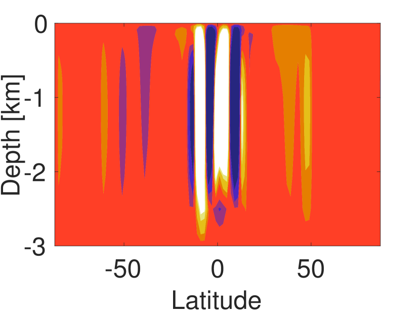
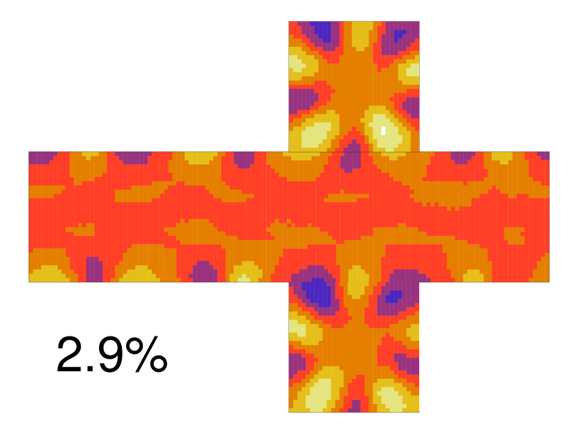
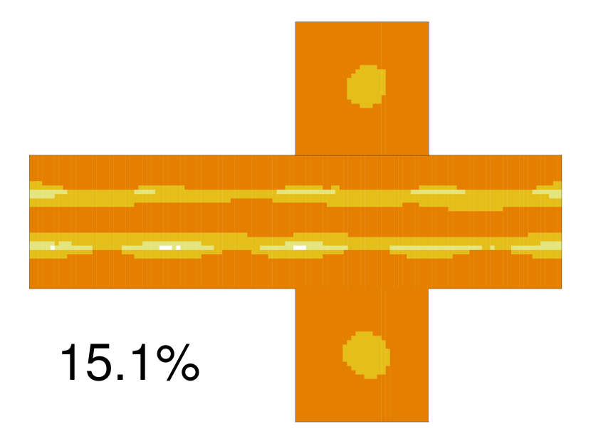
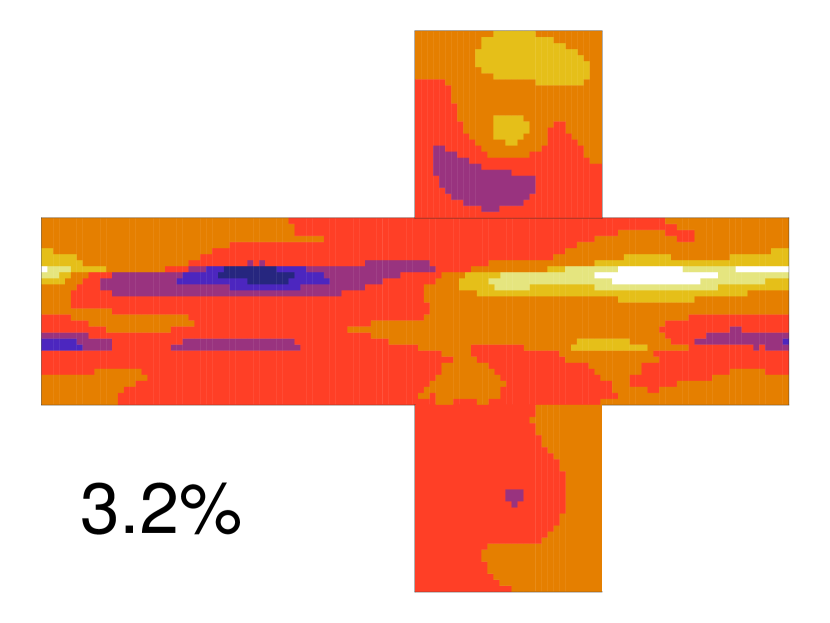
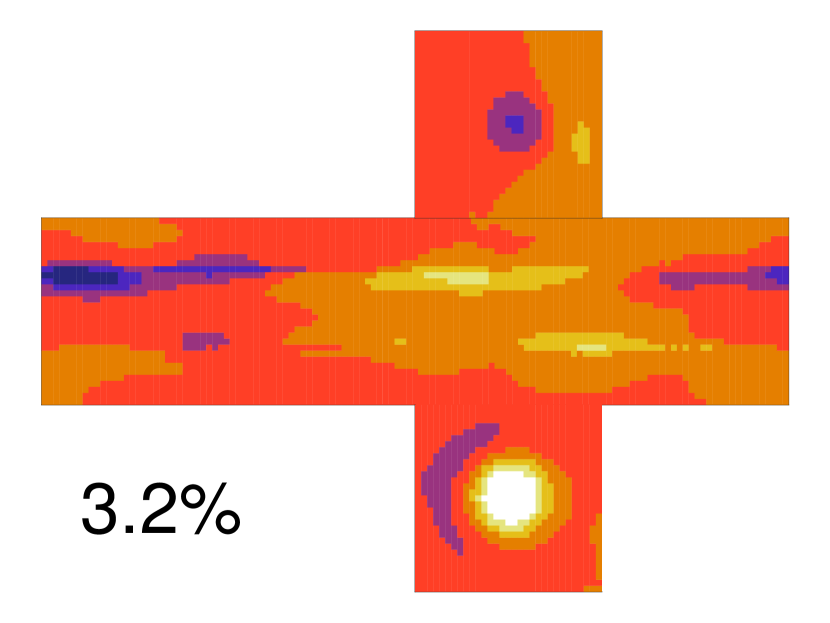
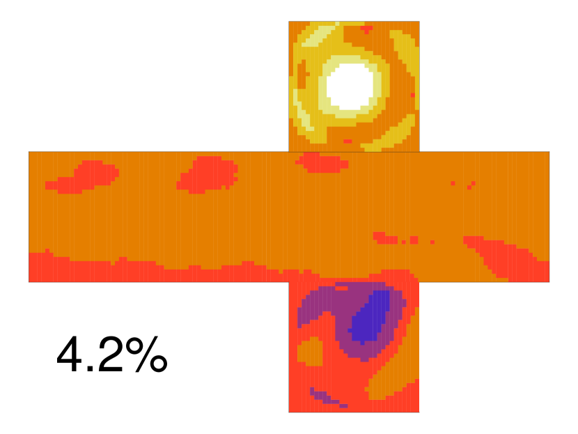
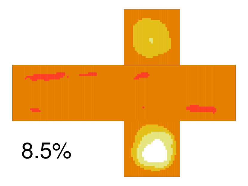
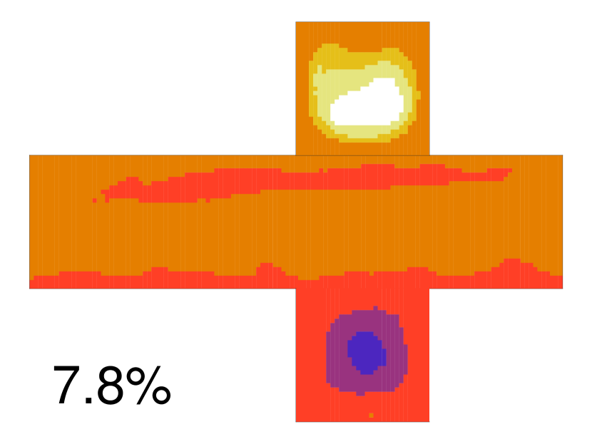
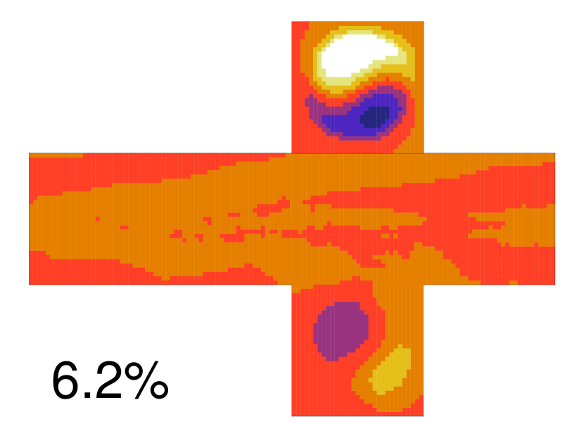
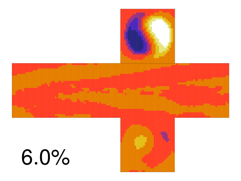
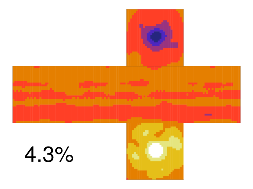
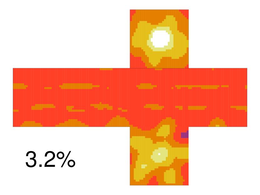
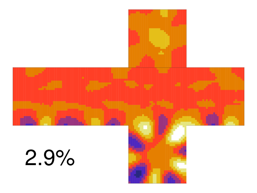
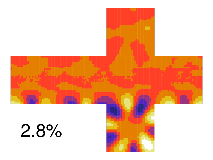
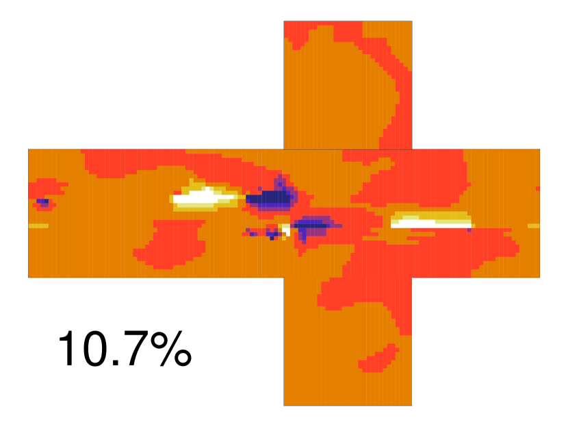
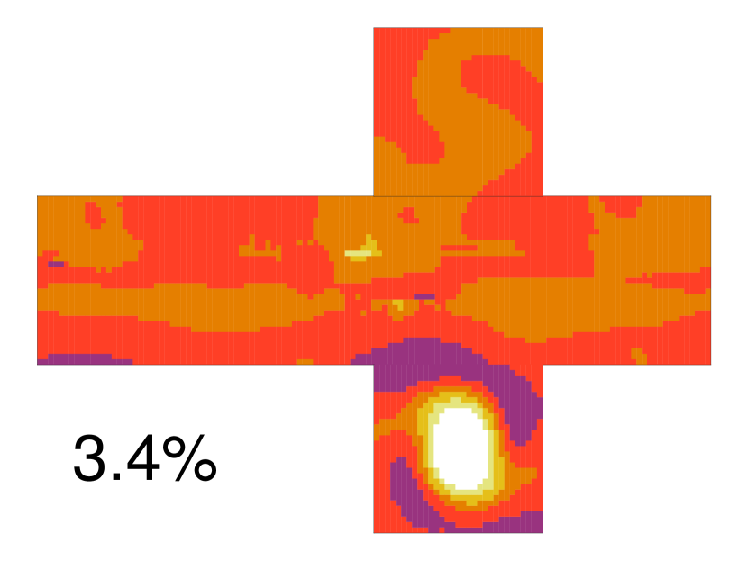
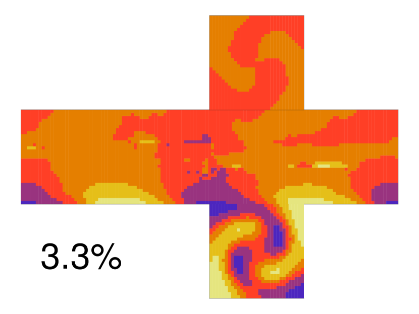
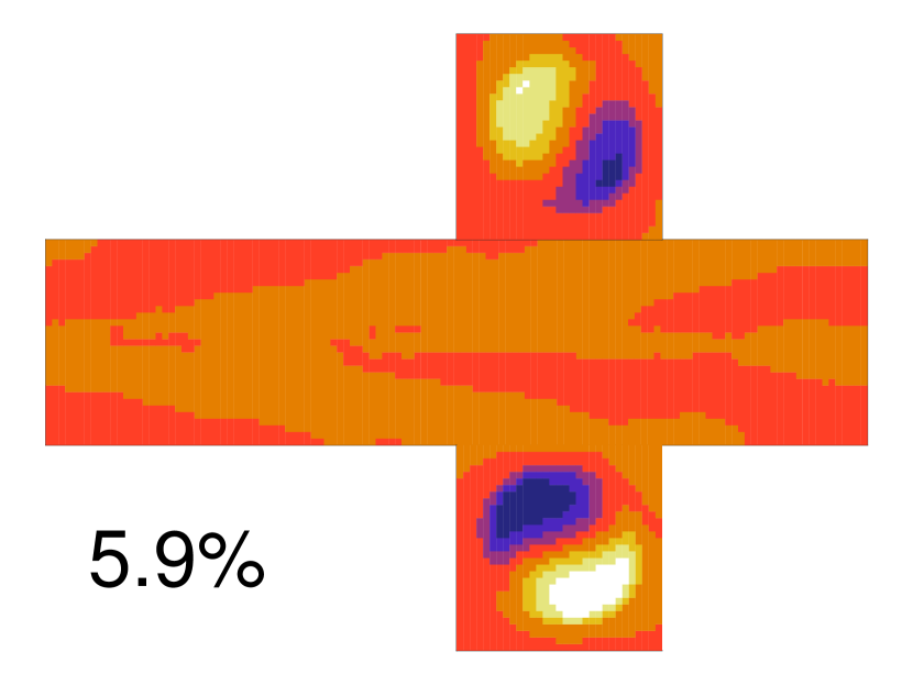
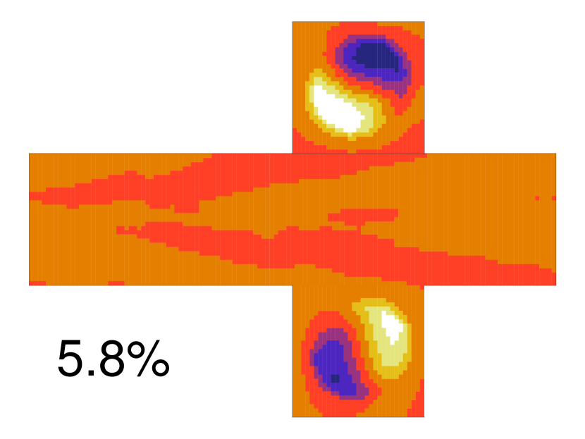
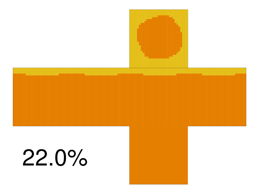
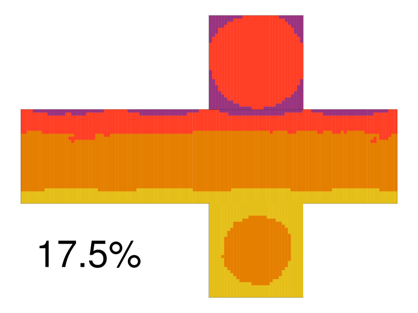
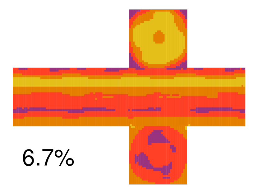
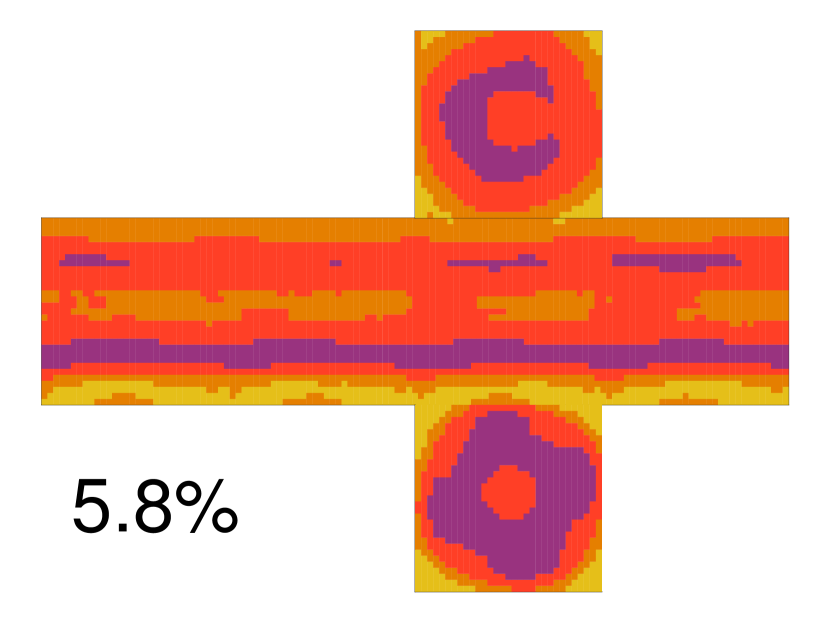
Fig. 7 displays the map of the four most important PCs for each attractor observed in setUp1.
-
•
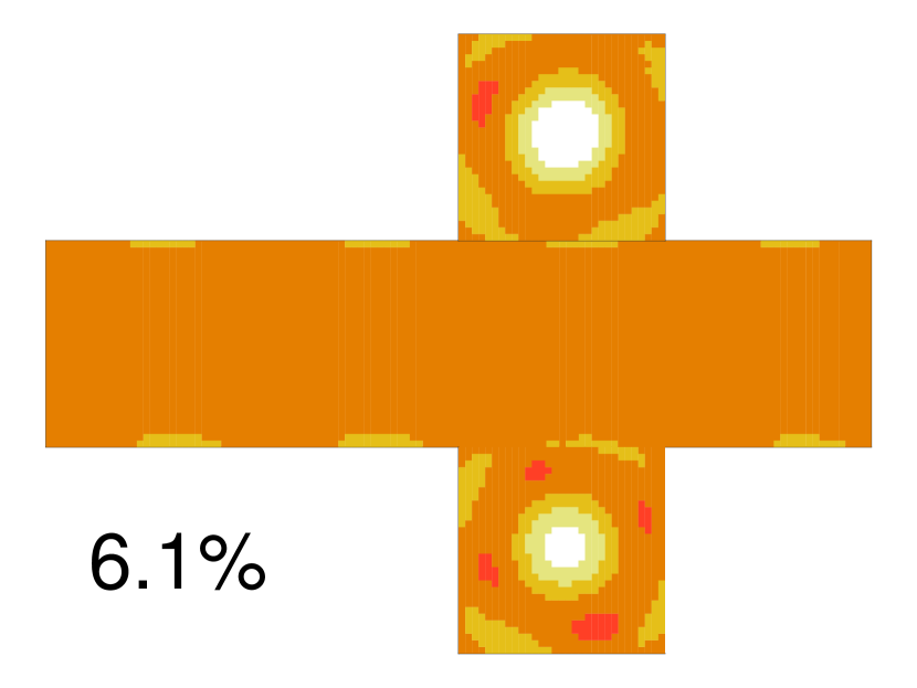
In the snowball, there are no modes describing more than 4% of the total variance, showing the lack of marked spatial dynamics in this regime and supporting the fact that the measure given by the instantaneous dimension is spurious, as discussed before and in agreement with Lucarini et al (2010); Lucarini and Bódai (2017). This is consistent with the very limited spatial heat transport, both in the ocean and in the atmosphere (Fig. 3, fourth column). However, the main feature (first two PCs) appears to be an opposition between the poles. The subsequent modes display rotating features in both polar regions.
-
•
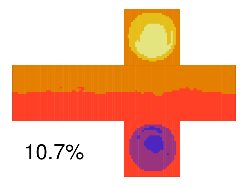
In the waterbelt, the four main modes display strong features around the tropics, evidencing that the dynamics occurs more at low latitudes, as opposed to the high-latitude dynamics of the cold and warm states. The first mode largely dominates the dynamics (15.1% of the variance, as compared to 3.2% for the second and third ones). Its main feature is a homogeneous positive sign indicating that the temperature variations are positively correlated across the whole Earth. The two rings around 16∘ latitude (close to the ice boundary, see Table 2) are more positive than the other regions, indicating wider temperature fluctuations consistent with the locally strong temperature gradient (see Fig. 3-4, first column), that also determines the high value of the instantaneous dimension. Therefore, the main driver of the inter-decadal variability in the waterbelt appears to be fluctuations of the sea ice edge (Rose, 2015).
-
•
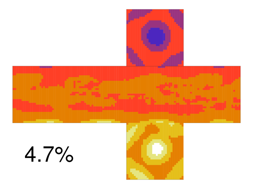
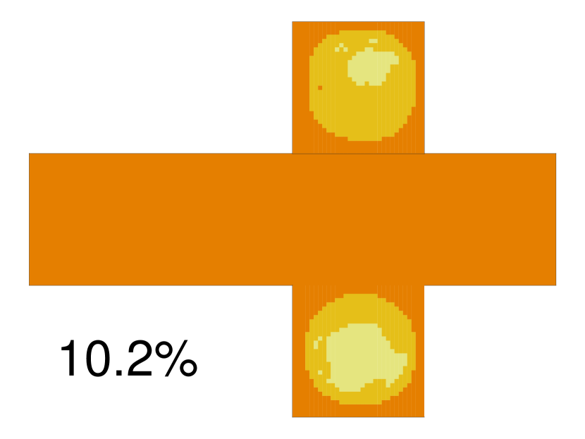
In the cold state, the dynamics displays more or less independent poles, with modes displaying pairwise symmetry: modes 1 and 2, and 3 and 4, each pair with similar explained variance. The first pair displays an opposition between a pole and its surrounding, around 65∘ latitude, as evidenced by the positive regions surrounded by a strongly negative ring. The pattern in the cloud cover shows a strong gradient at such latitudes (see Fig. 2, second column), suggesting an increasing relevance of the cloud albedo feedback in this attractor with respect to the ice albedo feedback, that is dominant in the previous attractors. This pair of modes also displays variability at midlatitudes that can be the signature for the modulation of the jet stream and the associated surface wind stress giving rise to the onset of oceanic and atmospheric annular modes, as discussed in Marshall et al (2007). The second pair of modes are weaker, and display two rings around the poles. They further contribute to this local dynamics in the subpolar region.
-
•
For the warm state, the first and second main modes have similar explained variance of the time series and correspond to temperature variations around the South (resp. North) pole, with a weak correlation in the first mode and anticorrelation in the second mode with the other pole. The four next modes point to independent dynamics in the polar regions, with a dominant vortical dynamics around the North pole for modes 3 and 4, and around the South pole for modes 5 and 6 (not shown).
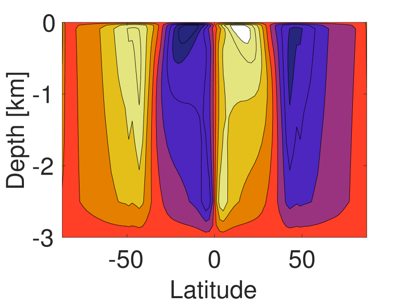
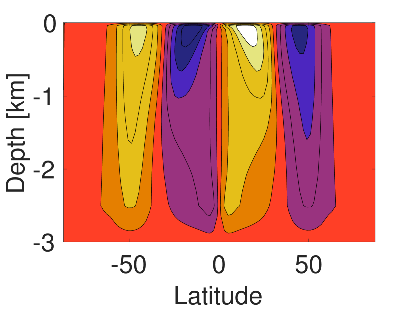
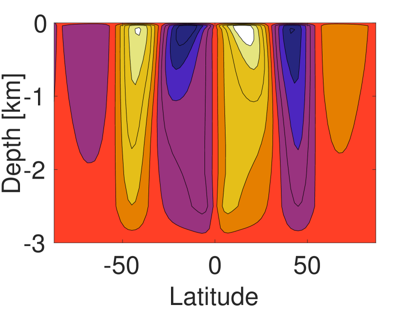
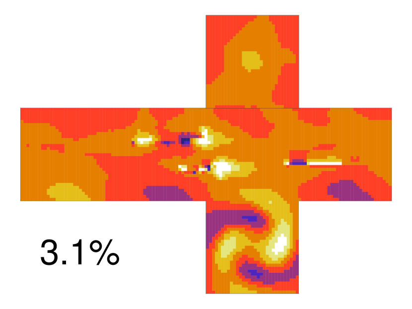
Switching off the latitude dependence of the bulk cloud albedo and the re-injection of dissipated kinematic energy (setUp2, Fig. 8) has very little influence on the PCA results for the snowball, with very little apparent structure, and for the cold state, with independent poles showing strong variability at high latitudes. The same similarity is observed in the warm state, where the inversion of the first two PCs is not relevant as these modes have equivalent weights. Furthermore, the rotating modes are also present in both set-ups. The PCs for the waterbelt are less similar in the two set-ups. However, like for setUp1, the first and widely dominating PC points to a strong dynamics in the tropical region at the edge of the sea ice cover, so that in both set-ups the fluctuations of the sea ice boundary turn out to be the main driver in this attractor. These similarities suggest that the additional processes considered in setUp1 and not in setUp2 have no qualitative influence on the dynamics of these attractors, although they affect their detailed quantitative properties.
Finally, the hot state is only observed in setUp2. It is characterised by weak fluctuations in the first mode, that represents 22% of the total variance, and by a high variability in the equatorial region in the subsequent modes, where the cloud cover is maximal (see Fig. 3, second column). This confirms the role of the cloud feedback in the dynamics of this attractor.
Mode 1
Mode 2
Mode 3
Mode 4

Snowball Waterbelt Cold state Warm state
Mode 1
Mode 2
Mode 3
Mode 4
Snowball Waterbelt Cold state Warm state Hot state
4 Discussion and conclusions
We have performed a systematic search of multiple-equilibria in an aquaplanet where the coupling between ocean, atmosphere and sea ice dynamics is simplified by the absence of continents. Similar attempts have been done in the past using a hierarchy of models of different complexity, ranging from energy balance models (Budyko, 1969; Sellers, 1969; Ghil, 1976; Abbot et al, 2011) and intermediate complexity models (Lucarini et al, 2010; Boschi et al, 2013; Lucarini and Bódai, 2017) to general circulation models (Ferreira et al, 2011; Rose, 2015). In these previous attempts, the model or the considered parameters range allowed for the presence of only a reduced number of attractors. To our knowledge, this is the first time that five attractors are obtained under the same external forcing, demonstrating that the unperturbed dynamics of general circulation models can be very complex. We have also shown in our simulations that by including a cloud albedo parameterisation that decreases the solar radiation in the polar regions, the number of attractors is reduced to four (the hot state disappears).
Each attractor is the result of the competition between different nonlinear mechanisms, in particular the ice-albedo feedback, the Boltzmann radiative feedback or the cloud feedback. Within the Solar system, several examples of astronomical objects can be found where one or the other nonlinear feedback dominates the global climate, even in the absence of multi-stability. In the CO2 atmosphere of Venus, a thick cloud layer with a maximum close to the tropical region induces a dominant cloud feedback as in the hot state, with surface temperatures as huge as 467∘C (Barstow et al, 2012). On Europa, one of the Jupiter moons, the surface is entirely covered by ice (Greenberg, 2002), like in the snowball, the final result of a dominant ice-albedo feedback. Exo-planets within our universe will likely provide other examples of extreme conditions and possible attractors in climate systems, enriching the number of possibilities.
The present work illustrates how complex is to construct the bifurcation diagram. Obtaining its full picture would require to systematically vary the external forcing by changing, for example, the inward solar radiation (Rose, 2015). Once the bifurcation diagram is obtained, one can start to investigate the response of the system to perturbations, especially relevant in the vicinity of tipping points. This will be investigated in forthcoming studies.
In the spirit of gradually increasing the complexity of the system (Jeevanjee et al, 2017), the same analysis may be repeated for configurations where the position of the continents plays a role in determining the number of attractors. First attempts with simplified continent distributions show the robustness of the attractors (Ferreira et al, 2011; Rose, 2015).
Different attractors have been recently proposed to co-exist in the Earth climate dynamics. Cold/hot states may correspond to glacial/interglacial cycles over the last three millions years (Ferreira et al, 2018). The shift between the two states may be triggered by internal variability, changes in internal feedbacks (for example variation of vegetation or ice cover) or in external forcing (such as Milankovitch cycles). The amplitude of the glacial/interglacial cycles is regular even if the incoming solar radiation is highly variable during glacial terminations (Petit et al, 1999), supporting the idea that such amplitude is connected to a property of the unperturbed dynamics. Similarly, beside the glacial/interglacial cycle, another cycle is proposed for the present-day climate that includes a hot state toward which the Earth System is approaching under the effect of global warming (Steffen et al, 2018). The discussion in Steffen et al (2018) is based on a qualitative analysis; here we have started to quantify the existence of such possible shift from a warm to a hot state starting from a simple aquaplanet configuration and we have shown that the appearance of the hot state strongly depends on the cloud parameterisation and on the amount of solar radiation entering in the polar regions.
A comprehensive understanding of attractors and their associated climates is key, in particular in the study of the geological past (i. e. Pohl et al (2014); Brunetti et al (2015); Ferreira et al (2018)). The study of the number and positions of climate attractors as defined herein can be applied to paleoclimate studies, in particular to geological periods where climatic shifts caused dramatic extinction events, like near the Permian-Triassic boundary. Adding the present analysis to the usual comparison with geological records of paleoclimate indicators, our confidence in retrieving the evolution of the climate of the Earth in deep past will be much enhanced.
Acknowledgements.
We acknowledge the financial support from the Swiss National Science Foundation (Sinergia Project CRSII5_180253). The computations were performed at University of Geneva on the Baobab and Climdal3 clusters. We are grateful to David Nagy, Carmelo E. Mileto and Enzo Putti-Garcia for running some of the simulations. We acknowledge an anonymous reviewer and Valerio Lucarini for helpful comments and suggestions. M. B. thanks Martin Beniston for inspiring discussions.References
- Abbot et al (2011) Abbot DS, Voigt A, Koll D (2011) The jormungand global climate state and implications for neoproterozoic glaciations. Journal of Geophysical Research 116:D18,103
- Adcroft et al (2004) Adcroft A, Campin JM, Hill C, Marshall J (2004) Implementation of an Atmosphere Ocean General Circulation Model on the Expanded Spherical Cube. Monthly Weather Review 132:2845, DOI 10.1175/MWR2823.1
- Barstow et al (2012) Barstow JK, Tsang CCC, Wilson CF, Irwin PGJ, Taylor FW, McGouldrick K, Drossart P, Piccioni G, Tellmann S (2012) Models of the global cloud structure on Venus derived from Venus Express observations. Icarus 217:542–560, DOI 10.1016/j.icarus.2011.05.018
- Bathiany et al (2016) Bathiany S, Dijkstra H, Crucifix M, Dakos V, Brovkin V, Williamson MS, Lenton TM, Scheffer M (2016) Beyond bifurcation: using complex models to understand and predict abrupt climate change. Dynamics and Statistics of the Climate System 1(1):dzw004, DOI 10.1093/climsys/dzw004, URL http://dx.doi.org/10.1093/climsys/dzw004
- Boccaletti et al (2005) Boccaletti G, Ferrari R, Adcroft A, Ferreira D, Marshall J (2005) The vertical structure of ocean heat transport. Geophysical Research Letters 32:L10603, DOI 10.1029/2005GL022474
- Boschi et al (2013) Boschi R, Lucarini V, Pascale S (2013) Bistability of the climate around the habitable zone: A thermodynamic investigation. Icarus 226:1724–1742, DOI 10.1016/j.icarus.2013.03.017, 1207.1254
- Brunetti and Vérard (2018) Brunetti M, Vérard C (2018) How to reduce long-term drift in present-day and deep-time simulations? Climate Dynamics 50:4425–4436, DOI 10.1007/s00382-017-3883-7, 1708.08380
- Brunetti et al (2015) Brunetti M, Vérard C, Baumgartner PO (2015) Modeling the Middle Jurassic ocean circulation. Journal of Palaeogeography 4:373–386
- Budyko (1969) Budyko MI (1969) The effect of solar radiation variations on the climate of the Earth. Tellus Series A 21:611–619, DOI 10.1111/j.2153-3490.1969.tb00466.x
- Caballero and Langen (2005) Caballero R, Langen PL (2005) The dynamic range of poleward energy transport in an atmospheric general circulation model. Geophysical Research Letters 32:L02705, DOI 10.1029/2004GL021581
- Dakos et al (2008) Dakos V, Scheffer M, van Nes EH, Brovkin V, Petoukhov V, Held H (2008) Slowing down as an early warning signal for abrupt climate change. Proceedings of the National Academy of Sciences 105(38):14308–14312, DOI 10.1073/pnas.0802430105, URL http://www.pnas.org/content/105/38/14308,
- Donohoe and Battisti (2012) Donohoe A, Battisti DS (2012) What Determines Meridional Heat Transport in Climate Models? Journal of Climate 25:3832–3850, DOI 10.1175/JCLI-D-11-00257.1
- Faranda et al (2017a) Faranda D, Messori G, Alvarez-Castro MC, Yiou P (2017a) Dynamical properties and extremes of Northern Hemisphere climate fields over the past 60 years. Nonlinear Processes in Geophysics 24:713–725, DOI 10.5194/npg-24-713-2017
- Faranda et al (2017b) Faranda D, Messori G, Yiou P (2017b) Dynamical proxies of North Atlantic predictability and extremes. Scientific Reports 7:41278, DOI 10.1038/srep41278
- Faranda et al (2019) Faranda D, Alvarez-Castro MC, Messori G, Rodrigues D, Yiou P (2019) The hammam effect or how a warm ocean enhances large scale atmospheric predictability. Nature Communications 10:1316, DOI 10.1038/s41467-019-09305-8
- Ferreira et al (2011) Ferreira D, Marshall J, Rose B (2011) Climate Determinism Revisited: Multiple Equilibria in a Complex Climate Model. Journal of Climate 24:992–1012, DOI 10.1175/2010JCLI3580.1
- Ferreira et al (2018) Ferreira D, Marshall J, Ito T, McGee D (2018) Linking glacial-interglacial states to multiple equilibria of climate. Geophysical Research Letters 45(17):9160–9170, DOI 10.1029/2018GL077019, URL https://agupubs.onlinelibrary.wiley.com/doi/abs/10.1029/2018GL077019
- Ferro and Segers (2003) Ferro CAT, Segers J (2003) Inference for clusters of extreme values. Journal Royal Statistical Society B 65:545–556, DOI 10.1111/1467-9868.00401
- Freitas et al (2010) Freitas ACM, Freitas JM, Todd M (2010) Hitting time statistics and extreme value theory. Probability Theory and Related Fields 147:675–710, DOI 10.1007/s00440-009-0221-y
- Gálfi et al (2017) Gálfi VM, Bódai T, Lucarini V (2017) Convergence of Extreme Value Statistics in a Two-Layer Quasi-Geostrophic Atmospheric Model. Complexity 2017:ID 5340,858, DOI 10.1155/2017/5340848
- Gallavotti (2006) Gallavotti G (2006) Stationary nonequilibrium statistical mechanics. Encyclopedia Math Phys 3:530–539
- Gent and McWilliams (1990) Gent PR, McWilliams JC (1990) Isopycnal Mixing in Ocean Circulation Models. Journal of Physical Oceanography 20:150–160
- Gent et al (2011) Gent PR, Danabasoglu G, Donner LJ, Holland MM, Hunke EC, Jayne SR, Lawrence DM, Neale RB, Rasch PJ, Vertenstein M, Worley PH, Yang ZL, Zhang M (2011) The Community Climate System Model Version 4. Journal of Climate 24:4973–4991, DOI 10.1175/2011JCLI4083.1
- Ghil (1976) Ghil M (1976) Climate Stability for a Sellers-Type Model. Journal of Atmospheric Sciences 33:3–20
- Grassberger and Procaccia (1983) Grassberger P, Procaccia I (1983) Characterization of strange attractors. Physical Review Letters 50:346–349, DOI 10.1103/PhysRevLett.50.346
- Greenberg (2002) Greenberg R (2002) Tides and the biosphere of europa: A liquid-water ocean beneath a thin crust of ice may offer several habitats for the evolution of life on one of jupiter’s moons. American Scientist 90(1):48–55, URL http://www.jstor.org/stable/27857596
- Held (2005) Held IM (2005) The gap between simulation and understanding in climate modeling. Bull Am Meteorological Soc 86:1609–1614, DOI 10.1175/BAMS-86-11-1609
- Jeevanjee et al (2017) Jeevanjee N, Hassanzadeh P, Hill S, Sheshadri A (2017) A perspective on climate model hierarchies. Journal of Advances in Modeling Earth Systems 9:1760–1771, DOI 10.1002/2017MS001038
- Kirschvink (1992) Kirschvink J (1992) Late Proterozoic Low-Latitude Global Glaciation: the Snowball Earth. In: The Proterozoic Biosphere: A Multidisciplinary Study, Cambridge University Press, New York, pp 51–52, URL https://authors.library.caltech.edu/36446/
- Kucharski et al (2006) Kucharski F, Molteni F, Bracco A (2006) Decadal interactions between the western tropical Pacific and the North Atlantic Oscillation. Climate Dynamics 26:79–91, DOI 10.1007/s00382-005-0085-5
- Kucharski et al (2013) Kucharski F, Molteni F, King MP, Farneti R, Kang IS, Feudale L (2013) On the need of intermediate complexity general circulation models: a speedy example. Bulletin of the American Meteorological Society 94(1):25–30, DOI 10.1175/BAMS-D-11-00238.1
- Large and Yeager (2004) Large WG, Yeager SG (2004) Diurnal to decadal global forcing for ocean and sea-ice models: the data sets and flux climatologies. NCAR Technical Note, NCAR, Boulder, CO
- Leadbetter (1983) Leadbetter MR (1983) Extremes and local dependence in stationary sequences. Z Wahrscheinlichkeitstheorie verw Gebiete 65:291–306, DOI 10.1007/BF00532484
- Lembo et al (2019) Lembo V, Lunkeit F, Lucarini V (2019) TheDiato (v1.0) - A new diagnostic tool for water, energy and entropy budgets in climate models. Geosci Model Dev Discuss URL https://doi.org/10.5194/gmd-2019-37
- Lenton et al (2008) Lenton TM, Held H, Kriegler E, Hall JW, Lucht W, Rahmstorf S, Schellnhuber HJ (2008) Tipping elements in the earth’s climate system. Proceedings of the National Academy of Sciences 105(6):1786–1793, DOI 10.1073/pnas.0705414105, URL http://www.pnas.org/content/105/6/1786, http://www.pnas.org/content/105/6/1786.full.pdf
- Lewis et al (2007) Lewis JP, Weaver AJ, Eby M (2007) Snowball versus slushball Earth: Dynamic versus nondynamic sea ice? Journal of Geophysical Research (Oceans) 112:C11014, DOI 10.1029/2006JC004037
- Lorenz (1963) Lorenz EN (1963) Deterministic Nonperiodic Flow. Journal of Atmospheric Sciences 20:130–148, DOI 10.1175/1520-0469(1963)020¡0130:DNF¿2.0.CO;2
- Lucarini and Bódai (2017) Lucarini V, Bódai T (2017) Edge states in the climate system: exploring global instabilities and critical transitions. Nonlinearity 30:R32, DOI 10.1088/1361-6544/aa6b11, 1605.03855
- Lucarini and Bódai (2019) Lucarini V, Bódai T (2019) Transitions across Melancholia States in a Climate Model: Reconciling the Deterministic and Stochastic Points of View. Physical Review Letters 122(15):158701, DOI 10.1103/PhysRevLett.122.158701, 1808.05098
- Lucarini and Pascale (2014) Lucarini V, Pascale S (2014) Entropy production and coarse graining of the climate fields in a general circulation model. Climate Dynamics 43:981–1000, DOI 10.1007/s00382-014-2052-5, 1304.3945
- Lucarini and Ragone (2011) Lucarini V, Ragone F (2011) Energetics of Climate Models: Net Energy Balance and Meridional Enthalpy Transport. Reviews of Geophysics 49:RG1001, DOI 10.1029/2009RG000323
- Lucarini et al (2010) Lucarini V, Fraedrich K, Lunkeit F (2010) Thermodynamic analysis of snowball Earth hysteresis experiment: Efficiency, entropy production and irreversibility. Quarterly Journal of the Royal Meteorological Society 136:2–11, DOI 10.1002/qj.543, 0905.3669
- Lucarini et al (2012) Lucarini V, Faranda D, Wouters J (2012) Universal Behaviour of Extreme Value Statistics for Selected Observables of Dynamical Systems. Journal of Statistical Physics 147:63–73, DOI 10.1007/s10955-012-0468-z, 1110.0176
- Lucarini et al (2014) Lucarini V, Blender R, Herbert C, Ragone F, Pascale S, Wouters J (2014) Mathematical and physical ideas for climate science. Reviews of Geophysics 52(4):809–859, DOI 10.1002/2013RG000446
- Lucarini et al (2016) Lucarini V, Faranda D, Freitas J, Holland M, Kuna T, Nicol M, Vaienti S (2016) Extremes and Recurrence in Dynamical Systems. Pure and Applied Mathematics: A Wiley Series of Texts, Monographs and Tracts, Wiley, URL https://books.google.ch/books?id=jRAiDAAAQBAJ
- Marshall et al (1997a) Marshall J, Adcroft A, Hill C, Perelman L, Heisey C (1997a) A finite-volume, incompressible Navier Stokes model for studies of the ocean on parallel computers. Journal of Geophysical Research 102:5753–5766, DOI 10.1029/96JC02775
- Marshall et al (1997b) Marshall J, Hill C, Perelman L, Adcroft A (1997b) Hydrostatic, quasi-hydrostatic, and nonhydrostatic ocean modeling. Journal of Geophysical Research 102:5733–5752, DOI 10.1029/96JC02776
- Marshall et al (2004) Marshall J, Adcroft A, Campin JM, Hill C (2004) Atmosphere-ocean modeling exploiting fluid isomorphisms. Monthly Weather Review 132:2882–2894
- Marshall et al (2007) Marshall J, Ferreira D, Campin JM, Enderton D (2007) Mean Climate and Variability of the Atmosphere and Ocean on an Aquaplanet. Journal of Atmospheric Sciences 64:4270, DOI 10.1175/2007JAS2226.1
- Milnor (1985) Milnor J (1985) On the concept of attractor. Communications in Mathematical Physics 99(2):177–195, DOI 10.1007/BF01212280
- Moloney et al (2019) Moloney NR, Faranda D, Sato Y (2019) An overview of the extremal index. Chaos 29(2):022101, DOI 10.1063/1.5079656
- Molteni (2003) Molteni F (2003) Atmospheric simulations using a GCM with simplified physical parametrizations. I: Model climatology and variability in multidecadal experiments. Climate Dynamics 20:175–191
- Nguyen et al (2011) Nguyen AT, Menemenlis D, Kwok R (2011) Arctic ice-ocean simulation with optimized model parameters: Approach and assessment. Journal of Geophysical Research (Oceans) 116:C04025, DOI 10.1029/2010JC006573
- Petit et al (1999) Petit JR, Jouzel J, Raynaud D, Barkov NI, Barnola JM, Basile I, Bender M, Chappellaz J, Davis M, Delaygue G, Delmotte M, Kotlyakov VM, Legrand M, Lipenkov VY, Lorius C, Pépin L, Ritz C, Saltzman E, Stievenard M (1999) Climate and atmospheric history of the past 420,000 years from the Vostok ice core, Antarctica. Nature 399:429–436, DOI 10.1038/20859
- Pierrehumbert et al (2011) Pierrehumbert R, Abbot D, Voigt A, Koll D (2011) Climate of the neoproterozoic. Annual Review of Earth and Planetary Sciences 39(1):417–460, DOI 10.1146/annurev-earth-040809-152447, URL https://doi.org/10.1146/annurev-earth-040809-152447
- Pohl et al (2014) Pohl A, Donnadieu Y, Le Hir G, Buoncristiani JF, Vennin E (2014) Effect of the Ordovician paleogeography on the (in)stability of the climate. Climate of the Past 10:2053–2066, DOI 10.5194/cp-10-2053-2014
- Poulsen et al (2001) Poulsen CJ, Pierrehumbert RT, Jacob RL (2001) Impact of ocean dynamics on the simulation of the neoproterozoic “snowball Earth”. Geophysical Research Letters 28:1575–1578, DOI 10.1029/2000GL012058
- Rose (2015) Rose BEJ (2015) Stable ‘WaterBelt’ climates controlled by tropical ocean heat transport: A nonlinear coupled climate mechanism of relevance to Snowball Eart. Journal of Geophysical Research: Atmospheres 120:1404–1423, DOI 10.1002/2014JD022659
- Rose and Marshall (2009) Rose BEJ, Marshall J (2009) Ocean Heat Transport, Sea Ice, and Multiple Climate States: Insights from Energy Balance Models. Journal of Atmospheric Sciences 66:2828, DOI 10.1175/2009JAS3039.1
- Rose et al (2013) Rose BEJ, Ferreira D, Marshall J (2013) The Role of Oceans and Sea Ice in Abrupt Transitions between Multiple Climate States. Journal of Climate 26:2862–2879, DOI 10.1175/JCLI-D-12-00175.1
- Saltzman (1983) Saltzman B (1983) Climatic Systems Analysis. Advances in Geophysics 25:173–233, DOI 10.1016/S0065-2687(08)60174-0
- Schubert and Lucarini (2016) Schubert S, Lucarini V (2016) Dynamical analysis of blocking events: spatial and temporal fluctuations of covariant Lyapunov vectors. Quarterly Journal of the Royal Meteorological Society 142:2143–2158, DOI 10.1002/qj.2808, 1508.04002
- Sellers (1969) Sellers WD (1969) A Global Climatic Model Based on the Energy Balance of the Earth-Atmosphere System. Journal of Applied Meteorology 8:392–400
- Shao (2017) Shao ZG (2017) Contrasting the complexity of the climate of the past 122,000 years and recent 2000 years. Scientific Report 7(4143):1–5, DOI 10.1038/s41598-017-04584-x
- Smith and Weissman (1994) Smith RL, Weissman I (1994) Estimating the extremal index. Journal Royal Statistical Society B 56(3):515–528
- Steffen et al (2018) Steffen W, Rockström J, Richardson K, Lenton TM, Folke C, Liverman D, Summerhayes CP, Barnosky AD, Cornell SE, Crucifix M, Donges JF, Fetzer I, Lade SJ, Scheffer M, Winkelmann R, Schellnhuber HJ (2018) Trajectories of the earth system in the anthropocene. Proceedings of the National Academy of Sciences 115(33):8252–8259, DOI 10.1073/pnas.1810141115, URL http://www.pnas.org/content/115/33/8252, http://www.pnas.org/content/115/33/8252.full.pdf
- Strogatz (1994) Strogatz SH (1994) Nonlinear dynamics and chaos, with applications to physics, biology, chemistry, and engineering. Westview Press
- Tang et al (2015) Tang L, Lv H, Yang F, Yu L (2015) Complexity testing techniques for time series data: A comprehensive literature review. Chaos Solitons and Fractals 81:117–135, DOI 10.1016/j.chaos.2015.09.002
- Tang et al (2016) Tang Y, Li L, Dong W, Wang B (2016) Reducing the climate shift in a new coupled model. Sci Bull 61:488–494, DOI 10.1007/s11434-016-1033-y
- Voigt and Abbot (2012) Voigt A, Abbot DS (2012) Sea-ice dynamics strongly promote snowball earth initiation and destabilize tropical sea-ice margins. Climate of the Past 8(6):2079–2092, DOI 10.5194/cp-8-2079-2012, URL https://www.clim-past.net/8/2079/2012/
- Wild et al (2013) Wild M, Folini D, Schär C, Loeb N, Dutton EG, König-Langlo G (2013) The global energy balance from a surface perspective. Climate Dynamics 40:3107–3134, DOI 10.1007/s00382-012-1569-8
- Winton (2000) Winton M (2000) A Reformulated Three-Layer Sea Ice Model. Journal of Atmospheric and Oceanic Technology 17:525–531
- Yang et al (2012) Yang J, Peltier WR, Hu Y (2012) The initiation of modern soft and hard Snowball Earth climates in CCSM4. Climate of the Past 8:907–918, DOI 10.5194/cp-8-907-2012