Device-Independent Quantum Private Query Protocol without the Assumption of Perfect Detectors

Abstract

The first device-independent quantum private query protocol (MRT17) which is proposed by Maitra et al. [Phys. Rev. A 95, 042344 (2017)] to enhance the security through the certification of the states and measurements. However, the MRT17 protocol works under an assumption of perfect detectors, which increases difficulty in the implementations. Therefore, it is crucial to investigate what would affect the security of this protocol if the detectors were imperfect. Meanwhile, Maitra et al. also pointed out that this problem remains open. In this paper, we analyze the security of MRT17 protocol when the detectors are imperfect and then find that this protocol is under attack in the aforementioned case. Furthermore, we propose device-independent QPQ protocol without the assumption of perfect detectors. Compared with MRT17 protocol, our protocol is more practical without relaxing the security in the device-independent framework.

I Introduction

Private information retrieval (PIR) 1 deals with the problem that an user (Alice) knows the address of an item from the database with $N$ items which is held by Bob and queries it secretly. In a PIR protocol, Alice gets correctly the item that she queried, whereas Bob does not know which item Alice has queried (i.e., the perfect user privacy). Furthermore, a symmetrically private information retrieval (SPIR) 2 has one more security requirement that Alice cannot get other items from the database except what she queried (i.e., the perfect database security). However, the task of SPIR cannot be realized ideally even in quantum cryptography 3 .

As a quantum protocol for dealing with SPIR problems, quantum private query (QPQ) relaxes the security requirements to some extent: i) Alice has nonzero probability to discover Bob’s attack if he attempts to learn the address of Alice’s queried item, which is referred to as cheat sensitivity. ii) Alice can gain a few more items than the perfect requirement where she only obtains the queried item.

In 2008, Giovannetti et al. 4 proposed the first cheat-sensitive QPQ protocol (GLM08), where the database was represented by a unitary operation (i.e., oracle operation) and it was performed on the query/test states at random, which were prepared by Alice. The query states were to obtain the retrieved item and the test states were to check potential attack from Bob. This protocol reduces exponentially the communication and computation complexity. Furthermore, the security of GLM08 protocol has been analyzed strictly 5 and a proof-of-principle experiment has been implemented 6 . Olejnik improved GLM08 protocol such that communication complexity was reduced further (O11)7 . These two protocols exhibit significant advantage in theory; but for large database dimension, these protocols are not practically implementable. To solve this problem, Jacobi et al. 8 proposed a QPQ protocol (J11) based on SARG04 quantum key distribution (QKD) protocol 9 , where this kind of protocols were called as QKD-based QPQ protocols. Compared with GLM08 and O11 protocols, J11 protocol can tolerate losses and be easily implemented to a database with large dimension. Subsequently, many QKD-based QPQ protocols 10 ; 11 ; 12 are proposed and their security either better users privacy or better database security even the perfect database security is studied 133 ; 13 ; 14 ; 144 . The development of QPQ protocols can be referred to 123 .

In the traditional QPQ protocol, Alice and Bob are required to trust their devices. If the states shared between them are not in the predetermined form, then Alice can always utilize some strategies which help her to elicit a few more items than what is suggested by the protocol. Thus, it is necessary for Bob to certify the states and measurements. With the advent of device-independent idea, the related cryptographic protocols do not rely on any assumptions about the states and measurements in their protocols. Zhao et al. 15 designed measurement device independence (MDI) QPQ protocol to certify the measurements (see Fig. 1). Later, Maitra, Paul and Roy proposed a device-independent (DI) QPQ protocol (MPR17) 16 to certify both states and measurements before proceeding to QPQ part (see Fig. 2).

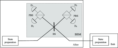
Figure 1: The framework of MDI QPQ. MDI indicates that measurement devices need not be characterized any more. The grey dotted box represents that Alice need not trust the Bell-state-measurement (BSM) device. BS and PBS represent the 50:50 beam splitter and polarization beam splitter, respectively.

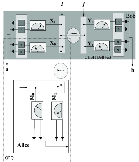
Figure 2: The framework of DI-QPQ. The grey box represents that Bob need not trust the device of states and measurements but certify the states and measurements via local CHSH Bell game. When the observed value violates the critical value of CHSH Bell game, QPQ part can be performed. Note that $\eta$ represents detection efficiency and assume $\eta=1$ in MRT17 protocol.

Obviously, MRT17 protocol enhances the security since the states and measurements need not be trusted but can be certified whether to be in a predetermined form. While, this protocol works under an assumption of perfect detectors (i.e., detectors with unit efficiency), which is hard to implement experimentally. If the assumption is relaxed, how will it affect the security of MRT17 protocol?

In this paper, we solve this problem and propose a DI-QPQ protocol without the assumption of perfect detectors. Firstly, we analyze security threat for MRT17 protocol under the case that the assumption is relaxed and the results show that this protocol is under attack in the above case. Secondly, we propose DI-QPQ protocols without the assumption of perfect detectors. Compared with MRT17 protocol, our protocol not only maintains the security in the DI framework but also is toward practical.

The remaining of the paper is as follows. The review of DI-QPQ protocol with an assumption of perfect detectors is given in Sect. II. DI-QPQ protocol without the assumption of perfect detectors is proposed and the security analysis is given in Sect. III. The conclusion is summarized in the last section.

II Review DI-QPQ protocol with the assumption of perfect detectors

The MRT17 protocol 16 is the first QPQ protocol in the DI framework. Our protocol is built on MRT 17 protocol. In this section, we revisit MRT17 (DI-QPQ) protocol 16 .

In the DI framework, the assumptions about states and measurements need not be made except for the basic ones. In the MRT17 protocol, the trustworthiness of Bob’s devices can be removed, and Bob utilizes a statistical method (known as CHSH Bell game) 17 to certify whether the shared states and measurements are in the predetermined forms between them.

Before introducing the details of MRT17 protocol, we give the relation between CHSH Bell test and CHSH Bell game.

In the standard CHSH Bell test,

1. $x_{i}\in\{0,1\}$ and $y_{i}\in\{0,1\}$ are chosen uniformly at random. $x_{i}=0(1)$ represents the measuring observables $\sigma_{z}(\sigma_{x})$; $y_{i}=0(1)$ represents the measuring observables $\frac{\sigma_{x}+\sigma_{z}}{\sqrt{2}}(\frac{\sigma_{z}-\sigma_{x}}{\sqrt{2}})$. The first and second particle of the entangled state can be measured, respectively. When the measurement result is $|0\rangle$ or $|+\rangle$ ($|1\rangle$ or $|-\rangle$), then $a_{i}=0(1)$. Similarly, the definition of $b_{i}$ has been given.

2. CHSH Bell correlation function is described as

   $$\begin{split}\hat{I}_{CHSH}&=E(X_{0}Y_{0})+E(X_{0}Y_{1})+E(X_{1}Y_{0})-E(X_{1}Y_{1}),\end{split}$$

   where

   $$E(X_{0}Y_{0})=\sum_{a_{i},b_{i}}(-1)^{a_{i}+b_{i}}p(a_{i},b_{i}|x_{i}=0,y_{i}=0),$$

   and others have similar definitions.

Now, if the shared state is $\frac{|00\rangle+|11\rangle}{\sqrt{2}}$, then $\hat{I}_{CHSH}=2\sqrt{2},$ which corresponds to the maximal violation in quantum theory.

In a general CHSH Bell test, the shared state is not the maximally entangled state but general entangled state and the measuring observables are $\{|\psi\rangle,|\psi^{\bot}\rangle\}$ for different four angles, where

$$\begin{split}&|\psi\rangle=\cos\frac{\psi}{2}|0\rangle+\sin\frac{\psi}{2}|1\rangle,\\ &|\psi^{\bot}\rangle=\sin\frac{\psi}{2}|0\rangle-\cos\frac{\psi}{2}|1\rangle.\\ \end{split}$$ (1)

thus $\hat{I}_{CHSH}\in(2,2\sqrt{2}]$ in quantum theory.

The CHSH Bell test is considered as a nonlocal game. Two players ($\mathfrak{P}_{1},\mathfrak{P}_{2}$) are viewed as cooperating with each other. A referee runs the game, and all communication is between the players and referee, while no communication directly between the players is permitted. The referee selects randomly $x_{i}y_{i}\in\{00,01,10,11\}$. Then, each player must answer a single bit ($a_{i}$ for $\mathfrak{P}_{1}$, $b_{i}$ for $\mathfrak{P}_{2}$). They win if $a_{i}+b_{i}=x_{i}\wedge y_{i}$. CHSH correlation function is characterized in the CHSH Bell test, while the average probability of success is described in the CHSH Bell game. The average probability of success$=\frac{1}{2}+\frac{\hat{I}_{CHSH}}{8},$ .

Next, we review the MRT17 protocol.

Firstly, the basic assumptions in the MRT17 protocol are listed 16 :

A

The additional information in Alice and Bob’s laboratories is not leaked.

B

Each use of device is independent of the previous uses.

C

All the detectors of Bob are perfect, i.e., unit efficiency.

The details of MRT17 protocol are introduced 16 .

1. Bob starts with $N$ entangled states which may be prepared by Alice.

2. Bob chooses some entangled states at random, which forms $\Gamma_{CHSH}$ for CHSH Bell test. $\Gamma_{CHSH}$ contains $\lceil\gamma N\rceil$ entangled states, where $0<\gamma<1$. The remained entangled states constitute $\Gamma_{QPQ}$ for QPQ protocol which contains $\lfloor(1-\gamma)N\rfloor$ entangled states.

3. For CHSH Bell game, $i\in\{1,...,\lceil\gamma N\rceil\}$,

   1. Bob chooses $x_{i}\in\{0,1\}$ and $y_{i}\in\{0,1\}$ uniformly at random.

   2. If $x_{i}=0(1)$, he measures the first particle of the entangled state in the basis $\{|0\rangle,|1\rangle\}(\{|+\rangle,|-\rangle\})$, then denote $a_{i}=0(1)$ when the measurement result is $|0\rangle$ or $|+\rangle$ ($|1\rangle$ or $|-\rangle$). In the same manner, if $y_{i}=0(1)$, he measures the second particle of the entangled state in the basis $\{|\psi_{1}\rangle,|\psi_{1}^{\bot}\rangle\}(\{|\psi_{2}\rangle,|\psi_{2}^{\bot}\rangle\})$, then denote $b_{i}=0(1)$ when the measurement result is $|\psi_{1}\rangle$ or $|\psi_{2}\rangle$ ($|\psi_{1}^{\bot}\rangle$ or $|\psi_{2}^{\bot}\rangle$), where

      $$\begin{split}&|\psi_{l}\rangle=\cos\frac{\psi_{l}}{2}|0\rangle+\sin\frac{\psi_{l}}{2}|1\rangle,\\ &|\psi_{l}^{\bot}\rangle=\sin\frac{\psi_{l}}{2}|0\rangle-\cos\frac{\psi_{l}}{2}|1\rangle\\ \end{split}$$ (2)

      for $l\in\{1,2\}$, $\psi_{1}\in(0,\frac{\pi}{2})$, $\psi_{2}\in(\frac{\pi}{2},\pi)$ and $\psi_{1}+\psi_{2}=\pi$.

   3. Statistical method 1: define $\mathcal{Y}_{i}$ be the observed result of the $i$th game for players, i.e.,

      $$\mathcal{Y}_{i}=\begin{cases}&1,\qquad\text{if}\quad a_{i}+b_{i}=x_{i}\wedge y_{i},\\ &0,\qquad\text{otherwise},\end{cases}$$ (3)

      and let $\mathcal{Y}$ be the average observed probability of success in the CHSH Bell game,

      $$\mathcal{Y}=\frac{1}{\lceil\gamma N\rceil}\sum_{i}\mathcal{Y}_{i}.$$ (4)

      If

      $$\mathcal{Y}<\bar{\mathcal{Y}},$$ (5)

      then Bob aborts the protocol, where $\bar{\mathcal{Y}}$ represents the average probability of success,

      $$\begin{split}\bar{\mathcal{Y}}=&\frac{1}{8}[\sin\theta(\sin\psi_{1}+\sin\psi_{2})+\cos\psi_{1}\\ &-\cos\psi_{2}]+\frac{1}{2}.\end{split}$$ (6)

      Otherwise, he proceeds to the following QPQ protocol 11 .

4. For QPQ part, the condition must be satisfied that the local CHSH Bell game at Bob’s end violates the above relation (5), thus the states shared between Alice and Bob are certified to be in their predetermined form, i.e.,

   $$\Psi_{BA}=\frac{1}{\sqrt{2}}(|0\rangle_{B}|\phi_{0}\rangle_{A}+|1\rangle_{B}|\phi_{1}\rangle_{A}),$$ (7)

   where

   $$|\phi_{0}\rangle_{A}=\cos\frac{\theta}{2}|0\rangle+\sin\frac{\theta}{2}|1\rangle,$$ (8)

   $$|\phi_{1}\rangle_{A}=\cos\frac{\theta}{2}|0\rangle-\sin\frac{\theta}{2}|1\rangle,$$ (9)

   for $\theta\in(0,\frac{\pi}{2})$.

   Next, Bob uses the remaining $\lfloor(1-\gamma)N\rfloor$ entangled pairs to proceed to QPQ steps.

   1. Bob sends a particle $A$ in each certified entangled pair (7) to Alice.

   2. Alice announces whether she has successfully received the particle or not. For un-received particle of Alice, Bob discards the corresponding particle.

   3. Then, Bob measures his particle in the basis $\{|0\rangle,|1\rangle\}$, Alice measures the corresponding particle in the basis $\{|\phi_{0}\rangle,|\phi_{0}^{\perp}\rangle\}$ or $\{|\phi_{1}\rangle,|\phi_{1}^{\perp}\rangle\}$. If Alice’s measurement outcome is $|\phi_{0}^{\perp}\rangle$ ( $|\phi_{1}^{\perp}\rangle$), she can conclude that the raw key bit at Bob’s end is 1 (0), and then the success probability that Alice gains a bit is showed in Table 1.

      Table 1: The success probability that Alice obtains a key.

      classical coding		0	1	1	0
      		$|\phi_{0}\rangle_{A}$	$|\phi_{0}^{\perp}\rangle_{A}$	$|\phi_{1}\rangle_{A}$	$|\phi_{1}^{\perp}\rangle_{A}$
      0	$\quad|0\rangle_{B}$	$\frac{1}{2}$	0	$\frac{1}{2}\cos^{2}\theta$	$\frac{1}{2}\sin^{2}\theta$
      1	$\quad|1\rangle_{B}$	$\frac{1}{2}\cos^{2}\theta$	$\frac{1}{2}\sin^{2}\theta$	$\frac{1}{2}$	0

   4. Alice’s measurements yield conclusive results and inconclusive ones. Both conclusive and inconclusive results are stored. Alice and Bob now share a raw key string (i.e., $K$). Bob knows the whole raw key string, whereas Alice generally knows the part of $K$, i,e., $\frac{\sin^{2}\theta}{2}|K|$, where $|K|$ represents the number of $K$.

   5. Alice and Bob postprocess $K$ so that Alice’s known key bits of $K$ are reduced to 1 bit.

   6. Bob encrypts his database so that Alice only obtains the item that she queried.

Different from traditional QPQ protocol, MRT17 protocol can certify whether the states and measurements to be in their predetermined forms. Thus, MRT17 protocol has an advantage of improving the security.

III DI-QPQ protocol without the assumption of perfect detectors

In this section, we discuss the security of MRT17 protocol when the assumption is relaxed. Then, we propose DI-QPQ protocol without the assumption of perfect detectors.

In general, the security analysis of QKD introduces an outside adversary (Eve) and investigates the effect of Eve’s attack, then rules out it. Different from QKD, each of the two parties may be an attacker for the counterpart in a QPQ protocol. Two cases are included in the security analysis: i) Alice tries to extract more information about the raw keys, or ii) Bob tries his best to learn the address of item that Alice queries.

III.1 The attack against MRT17 protocol if the detectors are imperfect

By considering a general attack scenario that Alice, as an adversary, tries to elicit more information from the raw keys, we discuss the security of MRT17 protocol with the assumption of perfect detectors via two statistical methods from CHSH Bell game/test, respectively. Furthermore, when the assumption is relaxed, we show that MRT17 protocol is under attack.

Suppose that Alice has ability to prepare the biased states such that the state is in the following form

$$\alpha|0\rangle_{B}|\phi_{0}\rangle_{A}+\beta|1\rangle_{B}|\phi_{1}\rangle_{A},$$ (10)

where

$$\begin{split}&\alpha=\sqrt{\frac{1}{2}+\epsilon},\qquad\beta=\sqrt{\frac{1}{2}-\epsilon},\\ &\epsilon\in(-\frac{1}{2},0)\cup(0,\frac{1}{2}),\end{split}$$ (11)

the difference between them lies in $\alpha,\beta$ compared with the predetermined state (7).

Firstly, we show that Alice’s attack does not work for MRT17 protocol with the assumption of perfect detector no matter which statistical method is from CHSH Bell game/test.

(1) the shared state in MRT17 protocol is certified in the way of nonlocal game.

After local CHSH Bell game, Bob gets

$$\begin{split}\mathcal{Y}&=\frac{1}{8}\sin\theta(\sin\psi_{1}+\sin\psi_{2})+\frac{\sqrt{\frac{1}{4}-\epsilon^{2}}}{4}(\cos\psi_{1}-\cos\psi_{2})\\ &\quad+\frac{1}{2},\end{split}$$ (12)

this value (12) cannot violate the condition (5) for an arbitrary value of $\epsilon$ (i.e., $\in(-\frac{1}{2},0)\cup(0,\frac{1}{2})$), and the proof is given Appendix A. According to the rules of MRT17 protocol, this protocol can be terminated. Obviously, Alice’s attack does not work for MRT17 protocol with the prefect detectors.

(2) the shared state in MRT17 protocol is certified in the way of CHSH Bell test. Statistical method of CHSH Bell test is in the following:

instead of steps (3)-(4), Statistical method 2: denote $I_{i}$ as the observed result in the $i$th experiment.

$$\begin{split}&I_{i}\\ &=\sum_{a_{i},b_{i},x_{i},y_{i}}(-1)^{a_{i}\oplus b_{i}\oplus x_{i}y_{i}}\frac{\chi(a_{i}=a,b_{i}=b,x_{i}=x,y_{i}=y)}{p(x_{i},y_{i})},\\ \end{split}$$ (13)

where

$$\chi(x)=\left\{\begin{array}[]{ll}1,&\hbox{$x$ is observed;}\\ 0,&\hbox{otherwise;}\end{array}\right.$$ (14)

$I_{CHSH}$ represents the observed value of CHSH Bell correlation function, i.e.,

$$I_{CHSH}=\frac{1}{\lceil\gamma N\rceil}\sum_{i=1}^{\lceil\gamma N\rceil}I_{i}.$$ (15)

When $N\rightarrow\infty$, $\hat{I}_{CHSH}$ can be represented as

$$\begin{split}\hat{I}_{CHSH}=&\frac{1}{\lceil\gamma N\rceil}\sum_{i=1}^{\lceil\gamma N\rceil}\sum_{a_{i},b_{i},x_{i},y_{i}}(-1)^{a_{i}+b_{i}+x_{i}y_{i}}\frac{\chi(a_{i}=a,}{}\\ &\quad\frac{b_{i}=b,x_{i}=x,y_{i}=y)}{p(x_{i},y_{i})}\\ =&\frac{1}{p(x_{i},y_{i})}\sum_{i=1}^{\lceil\gamma N\rceil}\sum_{a_{i},b_{i},x_{i},y_{i}}(-1)^{a_{i}+b_{i}+x_{i}y_{i}}\frac{\chi(a_{i}=a,}{}\\ &\quad\frac{b_{i}=b,x_{i}=x,y_{i}=y)}{\lceil\gamma N\rceil}\\ =&\frac{1}{p(x,y)}\sum_{a,b,x,y}(-1)^{a+b+xy}p(a,b,x,y)\\ =&\sum_{a,b,x,y}(-1)^{a+b+xy}p(a,b|x,y)\\ =&\sum_{a,b}(-1)^{a+b}[p(a,b|X_{0},Y_{0})+p(a,b|X_{0},Y_{1})+\\ &p(a,b|X_{1},Y_{0})-p(a,b|X_{1},Y_{1})\\ =&E(X_{0}Y_{0})+E(X_{0}Y_{1})+E(X_{1}Y_{0})-E(X_{1}Y_{1}).\end{split}$$ (16)

If

$$I_{CHSH}<\hat{I}_{CHSH},$$ (17)

where

$$\hat{I}_{CHSH}=\sin\theta(\sin\psi_{1}+\sin\psi_{2})+\cos{\psi_{1}-\cos{\psi_{2}}},$$ (18)

Bob aborts the protocol. Otherwise, Bob proceeds to the QPQ part. Note that the deduction of (18) can be referred to Appendix B.

Hence, based on the state (44) and statistical method 2, Bob gets

$$\begin{split}I_{CHSH}&=\sin\theta(\sin\psi_{1}+\sin\psi_{2})+2\sqrt{\frac{1}{4}-\epsilon^{2}}(\cos\psi_{1}\\ &\quad-\cos\psi_{2}).\end{split}$$ (19)

This value cannot violate the condition (17), the proof can be given in Appendix C.

To summarize, these two statistical methods can detect Alice’s attack that the states are not in the predetermined forms. These two statistical methods are equivalent.

Next, when the assumption is relaxed, we show that MRT17 protocol can be attacked successfully via Alice’s strategy that uses biased state (44).

We make use of statistical method 2 to catch the influence of the imperfect detectors. When the detection efficiency of Bob’s detectors is not limited to be unit, denoted as $\eta$, i.e.,

$$\eta=\min_{j,k}\{p(\Lambda_{X_{j}}),p(\Lambda_{Y_{k}})\}$$ (20)

where $\Lambda_{X_{j}}(\Lambda_{Y_{k}})$ represents the subensemble of nonempty outputs (i.e, $a(b)\in\{0,1\}$) when choosing measurement $X_{j}(Y_{k})$.

When the detectors are imperfect, the value of $I_{CHSH}$ with the biased state (44) is

$$\begin{split}I_{CHSH}&=\frac{8-2[\sin\theta(\sin\psi_{1}+\sin\psi_{2})+2\sqrt{\frac{1}{4}-\epsilon^{2}}}{\eta}\\ &\frac{(\cos\psi_{1}-\cos\psi_{2})]}{}+3[\sin\theta(\sin\psi_{1}+\sin\psi_{2})+\\ &2\sqrt{\frac{1}{4}-\epsilon^{2}}(\cos\psi_{1}-\cos\psi_{2})]-8.\end{split}$$ (21)

When $\eta$ and $\epsilon$ satisfy the following cases:

Case 1:

$$\begin{split}&\frac{2}{1+\sqrt{2}}<\eta<\frac{8-2A}{8-2A+B}<1,\\ &\epsilon\in(-\frac{1}{2},0)\cup(0,\frac{1}{2});\end{split}$$ (22)

Case 2:

$$\begin{split}&\frac{2}{1+\sqrt{2}}<\frac{8-2A}{8-2A+B}<\eta<\frac{8-2A-2B}{8-2A-2B},\\ &\epsilon\in(-\frac{\sqrt{(3\eta-2)^{2}B^{2}-C^{2}}}{2(3\eta-2)B},0)\cup(0,\frac{\sqrt{(3\eta-2)^{2}B^{2}-C^{2}}}{2(3\eta-2)B}),\end{split}$$ (23)

where

$$A=\sin\theta(\sin\psi_{1}+\sin\psi_{2}),$$ (24)

$$B=\cos\psi_{1}-\cos\psi_{2},$$ (25)

$$C=(8-2A+B)\eta-8+2A.$$ (26)

Eq.(21) violates the relation (17)(the proof is given in Appendix D), thus Bob proceeds to QPQ part. In the above cases, Alice successfully cheats Bob to make Bob believe that the states in his hand are in predetermined form which actually are not. In this way, the success probability of Alice’s guessing keys from the raw keys is $(\frac{1}{2}+2\epsilon^{2})\sin^{2}\theta$. Compared with $p=\frac{\sin^{2}\theta}{2}$, Alice successfully gets more information from Bob’s database without being caught. Therefore, when the detectors are not perfect, MRT17 protocol is insecure.

III.2 DI-QPQ protocol without the assumption of perfect detectors

According to the part A, we find that MRT17 protocol suffers an attack when the detectors are imperfect. How to design a DI-QPQ protocol without the assumption of perfect detectors becomes crucial. We rule out the influence of detector inefficiency and then propose DI-QPQ protocol without the assumption of perfect detectors. Our assumptions now are relaxed to the first two ones of MRT17 protocol. That is,

A

the additional information in Alice and Bob’s laboratories is no leaked.

B

each use of device is independent of the previous uses.

Denote the detection efficiency of Bob’s detectors as $\eta$. The procedures of DI-QPQ protocol without the assumption of perfect detectors are as follows:

1. Bob starts with $N$ entangled states which may be prepared by Alice.

2. Bob chooses some entangled states at random, which forms $\Gamma_{CHSH}$ for CHSH Bell test. $\Gamma_{CHSH}$ contains $\lceil\gamma N\rceil$ entangled states, where $0<\gamma<1$. The remained entangled states constitute $\Gamma_{QPQ}$ for QPQ protocol which contains $\lfloor(1-\gamma)N\rfloor$ entangled states.

3. For CHSH Bell test, $i\in\{1,...,\lceil\gamma N\rceil\}$,

   1. Bob chooses $x_{i}\in\{0,1\}$ and $y_{i}\in\{0,1\}$ uniformly at random.

   2. If $x_{i}=0(1)$, he measures the first particle of the entangled state in the basis $\{|0\rangle,|1\rangle\}(\{|+\rangle,|-\rangle\})$, then denotes $a_{i}=0(1)$ when the measurement result is $|0\rangle$ or $|+\rangle$ ($|1\rangle$ or $|-\rangle$). In the same manner, if $y_{i}=0(1)$, he measures the second particle of the entangled state in the basis $\{|\psi_{1}\rangle,|\psi_{1}^{\bot}\rangle\}(\{|\psi_{2}\rangle,|\psi_{2}^{\bot}\rangle\})$, then denotes $b_{i}=0(1)$ when the measurement result is $|\psi_{1}\rangle$ or $|\psi_{2}\rangle$ ($|\psi_{1}^{\bot}\rangle$ or $|\psi_{2}^{\bot}\rangle$), where

      $$\begin{split}&|\psi_{l}\rangle=\cos\frac{\psi_{l}}{2}|0\rangle+\sin\frac{\psi_{l}}{2}|1\rangle,\\ &|\psi_{l}^{\bot}\rangle=\sin\frac{\psi_{l}}{2}|0\rangle-\cos\frac{\psi_{l}}{2}|1\rangle\\ \end{split}$$ (27)

      for $l\in\{1,2\}$, $\psi_{1}\in(0,\frac{\pi}{2})$, $\psi_{2}\in(\frac{\pi}{2},\pi)$ and $\psi_{1}+\psi_{2}=\pi$.

   3. Statistical method 2:

      $$\begin{split}&I_{i}\\ &=\sum_{a_{i},b_{i},x_{i},y_{i}}(-1)^{a_{i}+b_{i}+x_{i}y_{i}}\frac{\chi(a_{i}=a,b_{i}=b,x_{i}=x,y_{i}=y)}{p(x_{i},y_{i})},\\ \end{split}$$ (28)

      where $I_{i}$ represents the observed result in the $i$th experiment.

      $$I_{CHSH}=\frac{1}{\lceil\gamma N\rceil}\sum_{i=1}^{\lceil\gamma N\rceil}I_{i},$$ (29)

      $I_{CHSH}$ represents the observed value of CHSH Bell correlation function.

   4. If

      $$I_{CHSH}<\bar{I}_{CHSH},$$ (30)

      where

      $$\begin{split}\bar{I}_{CHSH}&=-8+3[\sin\theta(\sin\psi_{1}+\sin\psi_{2})+\cos\psi_{1}-\cos\psi_{2}]\\ &\quad+\frac{8-2[\sin\theta(\sin\psi_{1}+\sin\psi_{2})+\cos\psi_{1}-\cos\psi_{2}]}{\eta},\end{split}$$ (31)

      $\bar{I}_{CHSH}$ represents the value of CHSH Bell correlation function.

   5. For QPQ part, the condition must be satisfied that the local CHSH Bell test at Bob’s end violates the above relation (30), thus the states shared between Alice and Bob are certified to be in their predetermined form, i.e.,

      $$\Psi_{BA}=\frac{1}{\sqrt{2}}(|0\rangle_{B}|\phi_{0}\rangle_{A}+|1\rangle_{B}|\phi_{1}\rangle_{A}),$$ (32)

      where

      $$|\phi_{0}\rangle_{A}=\cos\frac{\theta}{2}|0\rangle+\sin\frac{\theta}{2}|1\rangle,$$ (33)

      $$|\phi_{1}\rangle_{A}=\cos\frac{\theta}{2}|0\rangle-\sin\frac{\theta}{2}|1\rangle,$$ (34)

      for $\theta\in(0,\frac{\pi}{2})$.

      Next, Bob uses the remaining $\lfloor(1-\gamma)N\rfloor$ entangled pairs to proceed to QPQ steps which are the same as that of MRT17 protocol.

Note that the deduction of $\bar{I}_{CHSH}$ can be referred to Appendix E

In the following, we show the relation among $\theta$, detection efficiency ($\eta$) and the value of $\bar{I}_{CHSH}$ when $\psi_{1}=\pi/4,\psi_{2}=3\pi/4$ (see Fig. 3).

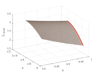
Figure 3: The relation among $\theta$, $\eta$ and the value of $\bar{I}_{CHSH}$ when $\psi_{1}=\pi/4,\psi_{2}=3\pi/4$. The red line represents the result of MRT17 protocol with assumption of perfect detectors.

From Fig. 3, the value of $\bar{I}_{CHSH}$ rules out the effect of detector inefficiency. When $I_{CHSH}=\bar{I}_{CHSH}$, the shared state is predetermined one; otherwise it is not. In particular, we show the relations between $\bar{I}_{CHSH}$ and $\theta$ when fixing the values of detection efficiency, i.e., $\eta=1,\ 0.83$, respectively.

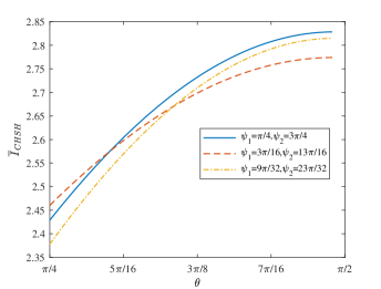
Figure 4: The relation between the value of $\bar{I}_{CHSH}$ and $\theta$ conditioned that $\eta=1$. The three lines represent these relations of different values of $(\psi_{1},\psi_{2})=(\pi/4,3\pi/4),(3\pi/16,13\pi/16)$ and $(9\pi/32,23\pi/32)$, respectively.

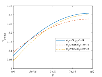
Figure 5: The relation between the value of $\bar{I}_{CHSH}$ and $\theta$ conditioned that $\eta=0.83$. The three lines represent these relations when $(\psi_{1},\psi_{2})=(\pi/4,3\pi/4),(3\pi/16,13\pi/16)$ and $(9\pi/32,23\pi/32)$, respectively.

III.3 Security Analysis

In this section, we analyze the security of our protocol.

Theorem 1

Suppose that there are $N$ pairs of entangled states in DI-QPQ protocol without the assumption of perfect detectors, these entangled states are divided randomly into two parts: $\Gamma_{CHSH}\subset\{1,\cdots,N\}$ of size $\lceil\gamma N\rceil$ with $0<\gamma<1$ and $\Gamma_{QPQ}=\{1,\cdots,N\}\backslash\Gamma_{CHSH}$.If

$$I_{CHSH}=\bar{I}_{CHSH}-\xi$$ (35)

is satisfied in the local CHSH Bell test, and then the relation (35) is still satisfied in the QPQ part with a negligible statistical deviation $v$, where $I_{CHSH}$ represents the observed value of CHSH Bell test, and $\bar{I}_{CHSH}$ represents the value of CHSH Bell test in predetermined states and measurements in our protocol.

$$\begin{split}\xi=\sqrt{\frac{1}{2\lceil\gamma N\rceil}\ln\frac{1}{\varepsilon_{CHSH}}},\\ v=\sqrt{\frac{(N-\lceil\gamma N\rceil+1)\lfloor(1-\gamma)N\rfloor^{2}\ln\frac{1}{\varepsilon_{QPQ}}}{2\lceil\gamma N\rceil N^{3}}},\end{split}$$ (36)

$\varepsilon_{CHSH}$ and $\varepsilon_{QPQ}$ are negligible small values.

proof: Different from the proof of MRT17 protocol, $I_{i}$ can be rewritten as

$$I_{i}=\begin{cases}\frac{(-1)^{a+b+xy}}{p(x,y)},&\text{if}\ (a_{i},b_{i},x_{i},y_{i})=(a,b,x,y)\ \text{is observed;}\\ 0,&\text{otherwise.}\\ \end{cases}\\$$ (37)

Then, $I_{CHSH}=\frac{1}{\lceil\gamma N\rceil}\sum_{i\in\Gamma_{CHSH}}I_{i}$ is called as the observed average value. The expected value of $I_{CHSH}$ is $\bar{I}_{CHSH}$.

Based on the Chernoff-Hoeffding bound 18 , we get

$$p(|I_{CHSH}-\bar{I}_{CHSH}|\geq\xi)\leq\exp(-2\xi^{2}\lceil\gamma N\rceil).$$ (38)

Let $\varepsilon_{CHSH}=\exp(-2\xi^{2}\lceil\gamma N\rceil)$, we get

$$\xi=\sqrt{\frac{1}{2\lceil\gamma N\rceil}\ln\frac{1}{\varepsilon_{CHSH}}}.$$ (39)

Further, denote $I^{\prime}_{CHSH}=\frac{1}{\lfloor(1-\gamma)N\rfloor}\sum_{i\in\Gamma_{QPQ}}I_{i}$ and $I=\frac{1}{N}\sum_{i\in\{1,...,N\}}I_{i}$, we have

$$p(|I_{CHSH}-I|\geq v)\leq\exp(\frac{-2v^{2}\lceil\gamma N\rceil N}{N-\lceil\gamma N\rceil+1}),$$ (40)

Due to $I=\frac{1}{N}\sum_{i\in\{1,...,N\}}I_{i}=\frac{\lceil\gamma N\rceil}{N}I_{CHSH}+\frac{\lfloor(1-\gamma)N\rfloor}{N}I^{\prime}_{CHSH}$, Eq. (40) can be rewritten as

$$\begin{split}&p(|I_{CHSH}-I|\geq v)\\ &=p(|I_{CHSH}-\frac{\lceil\gamma N\rceil}{N}I_{CHSH}-\frac{\lfloor(1-\gamma)N\rfloor}{N}I^{\prime}_{CHSH}|\geq v)\\ &=p(|\frac{\lfloor(1-\gamma)N\rfloor}{N}(I_{CHSH}-I^{\prime}_{CHSH})|\geq v)\\ &\leq\exp(\frac{-2v^{2}\lceil\gamma N\rceil N}{N-\lceil\gamma N\rceil+1}).\end{split}$$ (41)

Then, we have

$$p(|I_{CHSH}-I^{\prime}_{CHSH}|\geq\frac{N}{\lfloor(1-\gamma)N\rfloor}v)\leq\varepsilon_{QPQ},$$ (42)

Let $\varepsilon_{QPQ}=\exp(\frac{-2v^{2}\lceil\gamma N\rceil N^{3}}{(N-\lceil\gamma N\rceil+1)\lfloor(1-\gamma)N\rfloor^{2}})$, hence,

$$v=\sqrt{\frac{(N-\lceil\gamma N\rceil+1)\lfloor(1-\gamma)N\rfloor^{2}\ln\frac{1}{\varepsilon_{QPQ}}}{2\lceil\gamma N\rceil N^{3}}}.$$ (43)

$\sqcap$$\sqcup$

proposition 1

For DI-QPQ protocol without the assumption of perfect detectors, under the condition that the relation $I_{CHSH}<\bar{I}_{CHSH}$ is violated for the subset $\Gamma_{CHSH}$, Bob can proceed to the QPQ part for the remaining subset $\Gamma_{QPQ}$ securely when $N\rightarrow\infty$.

Note that $\Gamma_{CHSH}(\Gamma_{QPQ})$ represents the subset of entangled states that performs the local CHSH Bell test(QPQ part), $I_{CHSH}$ represents the observed value of CHSH Bell correlation function, and $\bar{I}_{CHSH}$ represents the value of CHSH Bell correlation function in predetermined states and measurements.

To sum up, on the basis of Theorem 1, when $N\rightarrow\infty$, the expression of $\xi$ tends to 0. This indicates that the certified states in the $\Gamma_{CHSH}$ are in the predetermined form. Furthermore, the states in the $\Gamma_{QPQ}$ can be certified, although the states in the $\Gamma_{QPQ}$ are not executed local CHSH Bell test. Associated with proposition 1, our protocol is secure.

IV Discussion and Conclusions

IV.1 Discussion

When the state shared Alice and Bob is $\epsilon$-close to the one given in Eq.(7), our protocol also works.

The state shared between them is descried as

$$\alpha|0\rangle_{B}|\phi_{0}\rangle_{A}+\beta|1\rangle_{B}|\phi_{1}\rangle_{A},$$ (44)

where

$$\begin{split}&\alpha=\sqrt{\frac{1}{2}+\epsilon},\qquad\beta=\sqrt{\frac{1}{2}-\epsilon},\\ &\epsilon\in(-\frac{1}{2},0)\cup(0,\frac{1}{2}),\end{split}$$ (45)

denoted as $\widetilde{\Psi}\rangle_{BA}$. When $\epsilon=0$, then $\widetilde{\Psi}\rangle_{BA}=\Psi\rangle_{BA}$.

If Alice and Bob agree to use $\widetilde{\Psi}\rangle_{BA}$ for performing our protocol, our protocol is unchanging except for the value $\bar{I}_{CHSH}$. the value $\bar{I}_{CHSH}$ is changed to

$$\begin{split}\bar{I}_{CHSH}=&\frac{8-2[\sin\theta(\sin\psi_{1}+\sin\psi_{2})+2\alpha\beta}{\eta}\\ &\frac{(\cos\psi_{1}-\cos\psi_{2})]}{}+3[\sin\theta(\sin\psi_{1}+\sin\psi_{2})+\\ &2\alpha\beta(\cos\psi_{1}-\cos\psi_{2})]-8.\end{split}$$ (46)

When completing this protocol, Bob knows that the number of Alice’s exacted keys is $(\frac{1}{2}+2\epsilon^{2})\sin^{2}\theta|K|$. Thus, Bob utilizes a suitable postprocessing such that Alice’s known key bits are reduced to 1 bit. Obviously, Alice does not obtain more items than the item that she queried. Further, this protocol is secure.

It is not hard to find that $\widetilde{\Psi}\rangle_{BA}$ is the same as the state in the adversary scenario in III.A. Compared with the case in adversary scenario, the difference lies in:

1)Alice and Bob agree to use $\widetilde{\Psi}\rangle_{BA}$ for carrying out DI-QPQ protocol;

2) Bob certifies whether the shared states are $\widetilde{\Psi}\rangle_{BA}$ or not;

3) Different from Eq.(6) and Eq.(18), the critical value (i.e., $\bar{I}_{CHSH}$) is changed;

4) Bob knows that the number of Alice’s known keys is not $\frac{\sin^{2}\theta}{2}|K|$ but $(\frac{1}{2}+2\epsilon^{2})\sin^{2}\theta|K|$, which helps to choose appropriate postprocessing.

IV.2 Conlusion

In this paper, we analyzed the security of MRT17 protocol when the detectors were imperfect and found this protocol was insecure in the above case. Furthermore, we proposed DI-QPQ protocol without the assumption of perfect detectors. Compared with MRT17 protocol, our protocol is towards practical and maintains the security in the DI framework.

But, some issues in DI-QPQ protocol are deserved to investigate in the future.

(1) Bell tests play an important role in the DI framework. While, Bell test encounters some loopholes such as free of choice loophole,detection loophole. We investigate or construct loophole-free Bell test to be adequate for DI-QPQ protocol.

(2) Novel DI-QPQ protocol which achieves better performance need be proposed. For example, a multi-bit block from the database in one query can be retrieved.

V Appendix

Appendix A: The result of Eq. (12) cannot violate the relation (5)

First, we give the deduction of Eq. (12) as follows.

$$\begin{split}&p(a_{i}\oplus b_{i}=x_{i}\wedge y_{i})\\ &=p_{X,Y}(0,0)[p(0,0|0,0)+p(1,1|0,0)]\\ &\quad+p_{X,Y}(0,1)[p(0,0|0,1)+p(1,1|0,1)]\\ &\quad+p_{X,Y}(1,0)[p(0,0|1,0)+p(1,1|1,0)]\\ &\quad+p_{X,Y}(1,1)[p(0,1|1,1)+p(1,0|1,1)]\\ &=\frac{1}{4}[\alpha^{2}\cos^{2}(\frac{\theta-\psi_{1}}{2})+\beta^{2}\sin^{2}(\frac{\theta+\psi_{1}}{2})]\\ &\quad+\frac{1}{4}[\alpha^{2}\cos^{2}(\frac{\theta-\psi_{2}}{2})+\beta^{2}\sin^{2}(\frac{\theta+\psi_{2}}{2})]\\ &\quad+\frac{1}{4}[(\frac{\alpha+\beta}{\sqrt{2}}\cos\frac{\psi_{1}}{2}\cos\frac{\theta}{2}+\frac{\alpha-\beta}{\sqrt{2}}\sin\frac{\psi_{1}}{2}\sin\frac{\theta}{2})^{2}\\ &\quad+(\frac{\alpha-\beta}{\sqrt{2}}\sin\frac{\psi_{1}}{2}\cos\frac{\theta}{2}-\frac{\alpha+\beta}{\sqrt{2}}\cos\frac{\psi_{1}}{2}\sin\frac{\theta}{2})^{2}]\\ &\quad+\frac{1}{4}[(\frac{\alpha+\beta}{\sqrt{2}}\sin\frac{\psi_{2}}{2}\cos\frac{\theta}{2}-\frac{\alpha-\beta}{\sqrt{2}}\cos\frac{\psi_{2}}{2}\sin\frac{\theta}{2})^{2}\\ &\quad+(\frac{\alpha-\beta}{\sqrt{2}}\cos\frac{\psi_{2}}{2}\cos\frac{\theta}{2}+\frac{\alpha+\beta}{\sqrt{2}}\sin\frac{\psi_{2}}{2}\sin\frac{\theta}{2})^{2}]\\ \end{split}$$ (47)

$$\begin{split}&=\frac{1}{8}\sin\theta(\sin\psi_{1}+\sin\psi_{2})+\frac{\sqrt{\frac{1}{4}-\epsilon^{2}}}{4}(\cos\psi_{1}-\cos\psi_{2})\\ &\quad+\frac{\cos\theta}{4}(\cos\psi_{1}+\cos\psi_{2})\epsilon+\frac{1}{2}\\ &=\frac{1}{8}\sin\theta(\sin\psi_{1}+\sin\psi_{2})+\frac{\sqrt{\frac{1}{4}-\epsilon^{2}}}{4}(\cos\psi_{1}-\cos\psi_{2})\\ &\quad+\frac{1}{2},\end{split}$$ (48)

where $p(0,0|0,0)=tr(|\Psi_{BA}\rangle\langle\Psi_{BA}||0\rangle\langle 0|\otimes|\psi_{1}\rangle\langle\psi_{1}|)$, other probabilities have similar operation method. The last equality holds since $\cos\psi_{1}+\cos\psi_{2}=0$.

Next, we prove that the above result cannot violate the relation (5). Denote the result of Eq. (12) as $f_{1}$, and let $\frac{1}{8}[\sin\theta(\sin\psi_{1}+\sin\psi_{2})+\cos\psi_{1}-\cos\psi_{2}]+\frac{1}{2}$ be $f_{0}$.

$$\begin{split}F(\epsilon)&=f_{1}-f_{0}\\ &=\frac{2\sqrt{\frac{1}{4}-\epsilon^{2}}-1}{8}(\cos\psi_{1}-\cos\psi_{2}).\end{split}$$ (49)

Via derivation of $F$ with respect to $\epsilon$, we get

$$F^{\prime}(\epsilon)=-\frac{1}{4}(\cos\psi_{1}-\cos\psi_{2})\frac{\epsilon}{\sqrt{\frac{1}{4}-\epsilon^{2}}}.$$ (50)

Case 1) when $\epsilon\in(0,\frac{1}{2})$, we get

$$\begin{split}&F^{\prime}(\epsilon)<0,\\ &F(0)=0.\end{split}$$ (51)

Case 2) when $\epsilon\in(-\frac{1}{2},0)$, we get

$$\begin{split}&F^{\prime}(\epsilon)>0,\\ &F(0)=0.\end{split}$$ (52)

Hence, when $\epsilon\in(-\frac{1}{2},0)\cup(0,\frac{1}{2})$, we get $F(\epsilon)<0$. That is, $f_{1}<f_{0}$. Therefore, Eq. (12) cannot violate the relation Eq. (5).     $\sqcap$$\sqcup$

Appendix B: the deduction of Eq. (18)

We deduce $E(X_{0}Y_{0})$, $E(X_{0}Y_{1})$, $E(X_{1}Y_{0})$ and $E(X_{1}Y_{1})$, respectively.

$$\begin{split}E(X_{0}Y_{0})&=\sum_{a,b\in\{0,1\}}(-1)^{ab}p(a,b|X_{0},Y_{0})\\ &=\sum_{a^{\prime},b^{\prime}\in\{1,-1\}}a^{\prime}b^{\prime}p(a^{\prime},b^{\prime}|X_{0},Y_{0})\\ &=p(1,1|X_{0},Y_{0})+p(-1,-1|X_{0},Y_{0})\\ &-p(-1,1|X_{0},Y_{0})-p(1,-1|X_{0},Y_{0})\\ &=\frac{1}{2}\cos^{2}(\frac{\theta-\psi_{1}}{2})+\frac{1}{2}\sin^{2}(\frac{\theta+\psi_{1}}{2})\\ &-\frac{1}{2}\sin^{2}(\frac{\theta-\psi_{1}}{2})-\frac{1}{2}\cos^{2}(\frac{\theta+\psi_{1}}{2})\\ &=\frac{1}{2}\cos(\theta-\psi_{1})-\frac{1}{2}\cos(\theta+\psi_{1})\\ &=\sin\theta\sin\psi_{1},\end{split}$$ (53)

where $p(1,1|X_{0},Y_{0})=tr(|\Psi_{BA}\rangle\langle\Psi_{BA}||0\rangle\langle 0|\otimes|\psi_{1}\rangle\langle\psi_{1}|)$, other probabilities have similar operation methods.

$$\begin{split}E(X_{0}Y_{1})&=\sum_{a^{\prime},b^{\prime}\in\{1,-1\}}a^{\prime}b^{\prime}p(a^{\prime},b^{\prime}|X_{0},Y_{1})\\ &=p(1,1|X_{0},Y_{1})+p(-1,-1|X_{0},Y_{1})\\ &-p(-1,1|X_{0},Y_{1})-p(1,-1|X_{0},Y_{1})\\ &=\frac{1}{2}\cos^{2}(\frac{\theta-\psi_{2}}{2})+\frac{1}{2}\sin^{2}(\frac{\theta+\psi_{2}}{2})\\ &-\frac{1}{2}\sin^{2}(\frac{\theta-\psi_{2}}{2})-\frac{1}{2}\cos^{2}(\frac{\theta+\psi_{2}}{2})\\ &=\frac{1}{2}\cos(\theta-\psi_{2})-\frac{1}{2}\cos(\theta+\psi_{2})\\ &=\sin\theta\sin\psi_{2},\end{split}$$ (54)

where $p(1,1|X_{0},Y_{1})=tr(|\Psi_{BA}\rangle\langle\Psi_{BA}||0\rangle\langle 0|\otimes|\psi_{2}\rangle\langle\psi_{2}|)$, other probabilities have similar operation methods.

$$\begin{split}E(X_{1}Y_{0})&=\sum_{a^{\prime},b^{\prime}\in\{1,-1\}}a^{\prime}b^{\prime}p(a^{\prime},b^{\prime}|X_{1},Y_{0})\\ &=p(1,1|X_{1},Y_{0})+p(-1,-1|X_{1},Y_{0})\\ &-p(-1,1|X_{1},Y_{0})-p(1,-1|X_{1},Y_{0})\\ &=\cos^{2}(\frac{\theta}{2})\cos^{2}(\frac{\psi_{1}}{2})+\sin^{2}(\frac{\theta}{2})\cos^{2}(\frac{\psi_{1}}{2})\\ &-\cos^{2}(\frac{\theta}{2})\sin^{2}(\frac{\psi_{1}}{2})-\sin^{2}(\frac{\theta}{2})\cos^{2}(\frac{\psi_{1}}{2})\\ &=\cos^{2}(\frac{\theta}{2})\cos(\psi_{1})+\sin^{2}(\frac{\theta}{2})\cos(\psi_{1})\\ &=\cos\psi_{1},\end{split}$$ (55)

where $p(1,1|X_{1},Y_{0})=tr(|\Psi_{BA}\rangle\langle\Psi_{BA}||+\rangle\langle+|\otimes|\psi_{1}\rangle\langle\psi_{1}|)$, other probabilities have similar operation methods.

$$\begin{split}E(X_{1}Y_{1})&=\sum_{a^{\prime},b^{\prime}\in\{1,-1\}}a^{\prime}b^{\prime}p(a^{\prime},b^{\prime}|X_{1},Y_{1})\\ &=p(1,1|X_{1},Y_{1})+p(-1,-1|X_{1},Y_{1})\\ &-p(-1,1|X_{1},Y_{1})-p(1,-1|X_{1},Y_{1})\\ &=\cos^{2}(\frac{\theta}{2})\cos^{2}(\frac{\psi_{2}}{2})+\sin^{2}(\frac{\theta}{2})\cos^{2}(\frac{\psi_{2}}{2})\\ &-\cos^{2}(\frac{\theta}{2})\sin^{2}(\frac{\psi_{2}}{2})-\sin^{2}(\frac{\theta}{2})\cos^{2}(\frac{\psi_{2}}{2})\\ &=\cos^{2}(\frac{\theta}{2})\cos(\psi_{1})+\sin^{2}(\frac{\theta}{2})\cos(\psi_{1})\\ &=\cos\psi_{2},\end{split}$$ (56)

where $p(1,1|X_{1},Y_{1})=tr(|\Psi_{BA}\rangle\langle\Psi_{BA}||+\rangle\langle+|\otimes|\psi_{2}\rangle\langle\psi_{2}|)$, other probabilities have similar operation methods.

Based on the above the results (53)-(56), we get

$$\begin{split}\hat{I}_{CHSH}&=E(X_{0}Y_{0})+E(X_{0}Y_{1})+E(X_{1}Y_{0})-E(X_{1}Y_{1})\\ &=\sin\theta(\sin\psi_{1}+\sin\psi_{2})+\cos\psi_{1}-\cos\psi_{2}.\end{split}$$ (57)

$\sqcap$$\sqcup$

Appendix C: Eq. (19) cannot violate the relation (17)

The deduction of (19) is similar to that of (18). Different from Eq. (18), the deduction of each probability term in Eq.(19) uses the state (44) instead of $|\Psi_{BA}\rangle$. Thus, we get

$$\begin{split}&E(X_{0}Y_{0})=\sin\theta\sin\psi_{1}+2\cos\theta\cos\psi_{1}\epsilon,\\ &E(X_{0}Y_{1})=\sin\theta\sin\psi_{2}+2\cos\theta\cos\psi_{2}\epsilon,\\ &E(X_{1}Y_{0})=2\sqrt{\frac{1}{4}-\epsilon^{2}}\cos\psi_{1},\\ &E(X_{1}Y_{1})=2\sqrt{\frac{1}{4}-\epsilon^{2}}\cos\psi_{2}.\\ \end{split}$$ (58)

Hence, we have

$$\begin{split}I_{CHSH}=&\sin\theta(\sin\psi_{1}+\sin\psi_{2})+2\cos\theta(\cos\psi_{1}+\cos\psi_{2})\epsilon\\ &+2\sqrt{\frac{1}{4}-\epsilon^{2}}(\cos\psi_{1}-\cos\psi_{2})\\ =&\sin\theta(\sin\psi_{1}+\sin\psi_{2})+2\sqrt{\frac{1}{4}-\epsilon^{2}}(\cos\psi_{1}-\cos\psi_{2}),\end{split}$$ (59)

the last equality holds since $\cos\psi_{1}+\cos\psi_{2}=0$.

Next, we prove that the above result cannot violate the relation (18). Denote the result of Eq. (19) as $g_{1}$, and let $\sin\theta(\sin\psi_{1}+\sin\psi_{2})+\cos\psi_{1}-\cos\psi_{2}$ be $g_{0}$.

$$\begin{split}F(\epsilon)&=g_{1}-g_{0}\\ &=(2\sqrt{\frac{1}{4}-\epsilon^{2}}-1)(\cos\psi_{1}-\cos\psi_{2}).\end{split}$$ (60)

Via derivation of $F$ with respect to $\epsilon$, we get

$$F^{\prime}(\epsilon)=-2(\cos\psi_{1}-\cos\psi_{2})\frac{\epsilon}{\sqrt{\frac{1}{4}-\epsilon^{2}}}.$$ (61)

Case 1) when $\epsilon\in(0,\frac{1}{2})$, we have

$$\begin{split}&F^{\prime}(\epsilon)<0,\\ &F(0)=0.\end{split}$$ (62)

Case 2) when $\epsilon\in(-\frac{1}{2},0)$, we have

$$\begin{split}&F^{\prime}(\epsilon)>0,\\ &F(0)=0.\end{split}$$ (63)

Hence, when $\epsilon\in(-\frac{1}{2},0)\cup(0,\frac{1}{2})$,we get $F(\epsilon)<0$. That is, $g_{1}<g_{0}$. In short, Eq. (19) cannot violate the relation Eq. (18).     $\sqcap$$\sqcup$

Appendix D: Eq. (21) violates the relation (17)

First, we deduce Eq. (21) in the following.

In the perfect detector scenario (i.e., $\eta=1$), when the state is in the form (44), Eq. (19) holds. When $\eta\neq 1$, Eq. (19) can be rewritten as

$$\begin{split}&E(X_{0}Y_{0}|\Lambda_{0})+E(X_{0}Y_{1}|\Lambda_{0})+E(X_{1}Y_{0}|\Lambda_{0})-E(X_{1}Y_{1}|\Lambda_{0})\\ &=\sin\theta(\sin\psi_{1}+\sin\psi_{2})+2\sqrt{\frac{1}{4}-\epsilon^{2}}(\cos\psi_{1}-\cos\psi_{2}),\end{split}$$ (64)

where $\Lambda_{0}=\Lambda_{X_{0}Y_{0}X_{1}Y_{1}}$ represents the ensemble that an arbitrary measurement pair gives the nonempty outcomes (i.e., $a^{\prime},b^{\prime}\in\{+1,-1\}$).

$E(X_{j}Y_{k}|\Lambda_{0})$ is inaccessible in the actual experiment, while $E(X_{j}Y_{k}|\Lambda_{X_{j}Y_{k}})$ is calculated easily in the above situation. So, in order to get the relation between $E(X_{j}Y_{k}|\Lambda_{0})$ and $E(X_{j}Y_{k}|\Lambda_{X_{j}Y_{k}})$, we define

$$\delta=\min_{(j,k)}p(\Lambda_{0}|\Lambda_{X_{j}Y_{k}}),$$ (65)

where $\min_{(j,k)}$ can be obtained by taking over all the measurement settings for $j,k\in\{0,1\}$.

The relation between $E(X_{j}Y_{k}|\Lambda_{X_{j}Y_{k}})$ and $E(X_{j}Y_{k}|\Lambda_{0})$ is given by

$$|E(X_{j}Y_{k}|\Lambda_{X_{j}Y_{k}})-\delta E(X_{j}Y_{k}|\Lambda_{0})|\leq 1-\delta$$ (66)

for $j,k\in\{0,1\}$.

proof Define $\overline{\Lambda_{0}}=\Lambda_{X_{j}Y_{k}}\setminus\Lambda_{0}$, which satisfies that

$$\begin{split}&\Lambda_{0}\cap\overline{\Lambda_{0}}=\emptyset,\\ &\Lambda_{0}\cup\overline{\Lambda_{0}}=\Lambda_{X_{j}Y_{k}}.\end{split}$$ (67)

Hence, we can get

$$\begin{split}&E(X_{j}Y_{k}|\Lambda_{X_{j}Y_{k}})=E(X_{j}Y_{k}|\overline{\Lambda_{0}}\cup\Lambda_{0})\\ =&p(\overline{\Lambda_{0}}|\Lambda_{X_{j}Y_{k}})E(X_{j}Y_{k}|\overline{\Lambda_{0}})+p(\Lambda_{0}|\Lambda_{X_{j}Y_{k}})E(X_{j}Y_{k}|\Lambda_{0}).\end{split}$$ (68)

Next, we have

$$\begin{split}&|E(X_{j}Y_{k}|\Lambda_{X_{j}Y_{k}})-\delta E(X_{j}Y_{k}|\Lambda_{0})|\\ =&|p(\overline{\Lambda_{0}}|\Lambda_{X_{j}Y_{k}})E(X_{j}Y_{k}|\overline{\Lambda_{0}})+p(\Lambda_{0}|\Lambda_{X_{j}Y_{k}})E(X_{j}Y_{k}|\Lambda_{0})\\ &-\delta E(X_{j}Y_{k}|\Lambda_{0})|\\ \leq&|p(\overline{\Lambda_{0}}|\Lambda_{X_{j}Y_{k}})E(X_{j}Y_{k}|\overline{\Lambda_{0}})|+|p(\Lambda_{0}|\Lambda_{X_{j}Y_{k}})E(X_{j}Y_{k}|\Lambda_{0})\\ &-\delta E(X_{j}Y_{k}|\Lambda_{0})|\\ \leq&p(\overline{\Lambda_{0}}|\Lambda_{X_{j}Y_{k}})E(|X_{j}Y_{k}||\overline{\Lambda_{0}})+(p(\Lambda_{0}|\Lambda_{X_{j}Y_{k}})-\delta)\\ &E(|X_{j}Y_{k}||\Lambda_{0})\\ \leq&1-\delta,\end{split}$$ (69)

where $E(|X_{j}Y_{k}|)=\sum_{a^{\prime},b^{\prime}}|a^{\prime}b^{\prime}|p(a^{\prime},b^{\prime}|X_{j},Y_{k})$. The first inequality holds based on $|x+y-z|\leq|x|+|y-z|$. The second inequality holds based on $|E(xy)|\leq E(|xy|)$. The last inequality holds on the basis of $E(|X_{j}Y_{k}||\overline{\Lambda_{0}})=1$ and $E(|X_{j}Y_{k}||\Lambda_{0})=1$ since $|a^{\prime}b^{\prime}|=1$ for $a^{\prime},b^{\prime}\in\{+1,-1\}$.     $\sqcap$$\sqcup$

Furthermore, in an actual experiment, we get

$$\begin{split}&I_{CHSH}\\ =&|E(X_{0}Y_{0}|\Lambda_{X_{0}Y_{0}})+E(X_{0}Y_{1}|\Lambda_{X_{0}Y_{1}})+E(X_{1}Y_{0}|\Lambda_{X_{1}Y_{0}})\\ &-E(X_{1}Y_{1}|\Lambda_{X_{1}Y_{1}})|\\ =&|E(X_{0}Y_{0}|\Lambda_{X_{0}Y_{0}})-\delta E(X_{0}Y_{0}|\Lambda_{0})+\delta E(X_{0}Y_{0}|\Lambda_{0})\\ +&E(X_{0}Y_{1}|\Lambda_{X_{0}Y_{1}})-\delta E(X_{0}Y_{1}|\Lambda_{0})+\delta E(X_{0}Y_{1}|\Lambda_{0})\\ +&E(X_{1}Y_{0}|\Lambda_{X_{1}Y_{0}})-\delta E(X_{1}Y_{0}|\Lambda_{0})+\delta E(X_{1}Y_{0}|\Lambda_{0})\\ -&(E(X_{1}Y_{1}|\Lambda_{X_{1}Y_{1}})+\delta E(X_{1}Y_{1}|\Lambda_{0})-\delta E(X_{1}Y_{1}|\Lambda_{0}))|.\end{split}$$ (70)

Via the property of the absolute value, Eq. (70) can be rewritten as

$$\begin{split}I_{CHSH}\leq&|E(X_{0}Y_{0}|\Lambda_{X_{0}Y_{0}})-\delta E(X_{0}Y_{0}|\Lambda_{0})|\\ &+|E(X_{0}Y_{1}|\Lambda_{X_{0}Y_{1}})-\delta E(X_{0}Y_{1}|\Lambda_{0})|\\ &+|E(X_{1}Y_{0}|\Lambda_{X_{1}Y_{0}})-\delta E(X_{1}Y_{0}|\Lambda_{0})|\\ &+|(E(X_{1}Y_{1}|\Lambda_{X_{1}Y_{1}})-\delta E(X_{1}Y_{1}|\Lambda_{0})|\\ &+\delta|E(X_{0}Y_{0}|\Lambda_{0})+E(X_{0}Y_{1}|\Lambda_{0})+E(X_{1}Y_{0}|\Lambda_{0})\\ &-E(X_{1}Y_{1}|\Lambda_{0})|.\\ \end{split}$$ (71)

By using Eq. (64) and Eq. (66), Eq. (71) can be deduced as

$$\begin{split}I_{CHSH}\leq&4(1-\delta)+[\sin\theta(\sin\psi_{1}+\sin\psi_{2})+2\sqrt{\frac{1}{4}-\epsilon^{2}}\\ &(\cos\psi_{1}-\cos\psi_{2})]\delta\\ =&4+[\sin\theta(\sin\psi_{1}+\sin\psi_{2})+2\sqrt{\frac{1}{4}-\epsilon^{2}}\\ &(\cos\psi_{1}-\cos\psi_{2})-4]\delta.\end{split}$$ (72)

Next, we give the relation between $\delta$ and detection efficiency $\eta$ as follow:

$$\delta\geq 3-\frac{2}{\eta}.$$ (73)

proof For $j^{\prime}\neq j$, $p(\Lambda_{X_{j^{\prime}}}|\Lambda_{X_{j}Y_{k}})$ is given by

$$\begin{split}&p(\Lambda_{X_{j^{\prime}}}|\Lambda_{X_{j}Y_{k}})=\frac{p(\Lambda_{X_{j^{\prime}}Y_{j}}|\Lambda_{Y_{k}})}{p(\Lambda_{X_{j}}|\Lambda_{Y_{k}})}\\ =&\frac{p(\Lambda_{X_{j^{\prime}}}|\Lambda_{B_{k}})+p(\Lambda_{X_{j}}|\Lambda_{Y_{k}})-p(\Lambda_{X_{j^{\prime}}}\cup\Lambda_{X_{j}}|\Lambda_{Y_{k}})}{p(\Lambda_{X_{j}}|\Lambda_{Y_{k}})}\\ \geq&\frac{2\eta-1}{\eta}.\end{split}$$ (74)

where we assume that the detection efficiency of each party is independent and constant rate, that is, $p(\Lambda_{X_{j^{\prime}}}|\Lambda_{Y_{k}})=p(\Lambda_{X_{j}}|\Lambda_{Y_{k}})=\eta$.

Furthermore, when $j^{\prime}\neq j$ and $k^{\prime}\neq k$, $p(\Lambda_{X_{j^{\prime}}Y_{k^{\prime}}}|\Lambda_{X_{j}Y_{k}})$ can be deduced by

$$\begin{split}p(\Lambda_{X_{j^{\prime}}Y_{k^{\prime}}}|\Lambda_{X_{j}Y_{k}})&=p(\Lambda_{X_{j^{\prime}}}|\Lambda_{X_{j}Y_{k}})+p(\Lambda_{Y_{k^{\prime}}}|\Lambda_{X_{j}Y_{k}})\\ &-p(\Lambda_{X_{j^{\prime}}}\cup\Lambda_{Y_{k^{\prime}}}|\Lambda_{X_{j}Y_{k}})\\ &\geq\frac{2\eta-1}{\eta}+\frac{2\eta-1}{\eta}-1\\ &=3-\frac{2}{\eta}.\end{split}$$ (75)

Finally, we calculate $\delta$. Without loss of generality, assume that $j=1,k=1$, $p(\Lambda_{0}|\Lambda_{X_{1}Y_{1}})$ can be represented as

$$\begin{split}&p(\Lambda_{0}|\Lambda_{X_{1}Y_{1}})=p(\Lambda_{X_{0}X_{1}Y_{0}Y_{1}}|\Lambda_{X_{1}Y_{1}})\\ =&p(\Lambda_{X_{0}Y_{0}}\cap\Lambda_{X_{1}Y_{1}}|\Lambda_{X_{1}Y_{1}})\\ =&p(\Lambda_{X_{0}Y_{0}}|\Lambda_{X_{1}Y_{1}})+p(\Lambda_{X_{1}Y_{1}}|\Lambda_{X_{1}Y_{1}})-p(\Lambda_{X_{0}Y_{0}}\cup\\ &\Lambda_{X_{1}Y_{1}}|\Lambda_{X_{1}Y_{1}})\\ \geq&p(\Lambda_{X_{0}Y_{0}}|\Lambda_{X_{1}Y_{1}})\\ \geq&3-\frac{2}{\eta},\end{split}$$ (76)

where the fifth line holds since $p(\Lambda_{X_{1}Y_{1}}|\Lambda_{X_{1}Y_{1}})=1,p(\Lambda_{X_{0}Y_{0}}\cup\Lambda_{X_{1}Y_{1}}|\Lambda_{X_{1}Y_{1}})\leq 1.$ The sixth line holds based on Eq. (75).

So, we get

$$\delta\geq 3-\frac{2}{\eta}.$$ (77)

$\sqcap$$\sqcup$

Input Eq. (73) into Eq. (72), we obtain

$$\begin{split}I_{CHSH}&\leq\frac{8-2[\sin\theta(\sin\psi_{1}+\sin\psi_{2})+2\sqrt{\frac{1}{4}-\epsilon^{2}}}{\eta}\\ &\quad\frac{(\cos\psi_{1}-\cos\psi_{2})]}{}-8+3[\sin\theta(\sin\psi_{1}+\sin\psi_{2})\\ &+2\sqrt{\frac{1}{4}-\epsilon^{2}}(\cos\psi_{1}-\cos\psi_{2})].\end{split}$$ (78)

Here, in order to demonstrate there exists an attack strategy, we only consider $I_{CHSH}=\frac{8-2[\sin\theta(\sin\psi_{1}+\sin\psi_{2})+2\sqrt{\frac{1}{4}-\epsilon^{2}}(\cos\psi_{1}-\cos\psi_{2})]}{\eta}-8+3[\sin\theta(\sin\psi_{1}+\sin\psi_{2})+2\sqrt{\frac{1}{4}-\epsilon^{2}}(\cos\psi_{1}-\cos\psi_{2})]$.

Next, we prove that the above value violates the relation (17) in some cases. Let

$$A=\sin\theta(\sin\psi_{1}+\sin\psi_{2}),$$ (79)

$$B=\cos\psi_{1}-\cos\psi_{2},$$ (80)

$$C=(8-2A+B)\eta-8+2A.$$ (81)

On the basis of 166 , the detection loophole of CHSH Bell test can be closed when $\eta>\frac{2}{1+\sqrt{2}}$.

(1) when $\eta<\frac{8-2A}{8-2A+B}$, we get

$$(8-2A+B)\eta-8+2A<0.$$ (82)

Now, when $\epsilon\in(-\frac{1}{2},0)\cup(0,\frac{1}{2})$, we get

$$2(3\eta-2)B\sqrt{\frac{1}{4}-\epsilon^{2}}>(8-2A+B)\eta-8+2A,$$ (83)

since $(3\eta-2)B\sqrt{\frac{1}{4}-\epsilon^{2}}>0$ and $(8-2A+B)\eta-8+2A<0$.

In the above case, we get

$$\begin{split}Eq.(\ref{e21})-Eq.(\ref{e5})&=\frac{2(3\eta-2)B\sqrt{\frac{1}{4}-\epsilon^{2}}-[(8-2A}{\eta}\\ &\frac{\quad+B)\eta+8-2A]}{}.\end{split}$$ (84)

On the basis of the relation (83), we know

$$Eq.(\ref{e21})-Eq.(\ref{e5})>0.$$ (85)

Hence, Eq. (21) can violate the relation Eq. (18) in the above case.

(2) when $\frac{8-2A}{8-2A+B}<\eta<\frac{8-2A-2B}{8-2A-2B}$, we get

$$(8-2A-B)\eta-8+2A>0,$$ (86)

$$(8-2A-2B)\eta<8-2A-2B.$$ (87)

Eq. (87) can be rewritten as $(3\eta-2)B-[(8-2A+B)\eta-8+2A]>0.$ That is, $(3\eta-2)B>C>0$.

Further, when $\epsilon\in(-\frac{\sqrt{(3\eta-2)^{2}B^{2}-C^{2}}}{2(3\eta-2)B},0)\cup(0,\frac{\sqrt{(3\eta-2)^{2}B^{2}-C^{2}}}{2(3\eta-2)B})$, we get

$$4(3\eta-2)^{2}B^{2}\epsilon^{2}<(3\eta-2)^{2}B^{2}-C^{2}.$$ (88)

So, we have

$$2(3\eta-2)B\sqrt{\frac{1}{4}-\epsilon^{2}}>C>0.$$ (89)

On the basis of the relation (89), we know

$$Eq.(\ref{e21})-Eq.(\ref{e5})>0.$$ (90)

Hence, Eq. (21) can violate the relation Eq. (17) in the above case.     $\sqcap$$\sqcup$

Appendix E: The deduction of Eq.(31)

In the perfect detector scenario ($\eta=1$), we can assert that Eq. (18) has self-tested the state and measurements in the predetermined forms. When $\eta$ is no larger than a certain value, Alice takes advantage of the detector inefficiency such that Bob still gets the result (18). In fact, the state and measurements are not in the predetermined form. Now, Alice can get more information about items without being discovered by Bob. In order to avoid this cheat strategy, more precisely, Eq. (18) can be rewritten as

$$\begin{split}&E(X_{0}Y_{0}|\Lambda_{0})+E(X_{0}Y_{1}|\Lambda_{0})+E(X_{1}Y_{0}|\Lambda_{0})-E(X_{1}Y_{1}|\Lambda_{0})\\ &=\sin\theta(\sin\psi_{1}+\sin\psi_{2})+\cos\psi_{1}-\cos\psi_{2},\end{split}$$ (91)

where $\Lambda_{0}=\Lambda_{X_{0}Y_{0}X_{1}Y_{1}}$ represents the ensemble that an arbitrary measurement pair gives the nonempty outcomes (i.e., $a^{\prime},b^{\prime}\in\{+1,-1\}$).

Next, the deduction of Eq. (31) is similar to that of Eq. (21). While, the difference between them lies in the relation (72). In the deduction of Eq. (31), $I_{CHSH}$ can be rewritten as

$$\begin{split}I_{CHSH}\leq&4(1-\delta)+[\sin\theta(\sin\psi_{1}+\sin\psi_{2})+\cos\psi_{1}-\cos\psi_{2}]\delta\\ =&4+[\sin\theta(\sin\psi_{1}+\sin\psi_{2})+\cos\psi_{1}-\cos\psi_{2}-4]\delta.\end{split}$$ (92)

Input Eq. (73) into Eq. (92), we obtain

$$\begin{split}I_{CHSH}&\leq\frac{8-2[\sin\theta(\sin\psi_{1}+\sin\psi_{2})+\cos\psi_{1}-\cos\psi_{2}]}{\eta}\\ &-8+3[\sin\theta(\sin\psi_{1}+\sin\psi_{2})+\cos\psi_{1}-\cos\psi_{2}].\end{split}$$ (93)

Hence, denote $\bar{I}_{CHSH}$ as $\frac{8-2[\sin\theta(\sin\psi_{1}+\sin\psi_{2})+\cos\psi_{1}-\cos\psi_{2}]}{\eta}$ $-8+3[\sin\theta(\sin\psi_{1}+\sin\psi_{2})+\cos\psi_{1}-\cos\psi_{2}]$.

$\sqcap$$\sqcup$

References

- (1) B. Chor, O. Goldreich, E. Kushilevitz, M. Sudan, J. ACM 45,965-981 (1998)
- (2) Y. Gertner, Y. Ishai, E. Kushilevitz, T. Malkin, J. Comput. Syst. Sci. 60, 592-629 (2000)
- (3) H. K. Lo, Phys. Rev. A 56, 1154-1162 (1997)
- (4) V. Giovannetti, S. Lloyd, L. Maccone, Phys. Rev. Lett. 100, 230502 (2008)
- (5) V. Giovannetti, S. Lloyd, L. Maccone, IEEE T. Inform. Theory 56, 3465-3477 (2010)
- (6) F. DeMartini, V. Giovannetti, S. Lloyd, L. Maccone, E. Nagali, L. Sansoni, F. Sciarrino, Phys. Rev. A 80,010302 (2009)
- (7) L. Olejnik, Phys. Rev. A 84, 022313 (2011)
- (8) M. Jakobi, C. Simon, N. Gisin, J. D. Bancal, C. Branciard, N. Walenta, H. Zbinden, Phys. Rev. A 80,022301(2009)
- (9) V. Scarani, A. Acín, G. Ribordy, N. Gisin, Phys. Rev. Lett. 92, 057901 (2004)
- (10) F. Gao, B. Liu, Q. Y. Wen, H. Chen, Opt. Express 20, 17411 (2012)
- (11) J. L. Zhang, F. Z. Guo, F. Gao, B. Liu, Q. Y. Wen, Phys. Rev. A 88, 022334 (2014)
- (12) Y. G. Yang, S. J. Sun, J. Tian, Quan. Inform. Procce. 13, 805-813 (2014)
- (13) F. Gao, B. Liu, W. Huang, and Q. Y. Wen, IEEE J. Sel. Top. Quant. 21,6600111 (2015).
- (14) P. Chan, I. X. Mo. Lucio-Martinezm , C. Simon, W. Tittel, Scientific Reports 4, 5233 (2014)
- (15) B. Liu, F. Gao, W. Huang, Q. Y. Wen, Science China Physics, Mechanics & Astronomy 58, 100301 (2015)
- (16) C. Y. Wei, X. Q. Cai, B. Liu, T. Y. Wang, and F. Gao, IEEE T. Comput. 67, 2 (2018).
- (17) F. Gao, S. J. Qin, W. Huang, Q.Y. Wen, Sci. China-Phys. Mech. Astron. 62, 70301 (2019).
- (18) L. Y. Zhao, Z. Q. Yin, W. Chen, Y. J. Qian, C. M. Zhang, G. C. Guo, Z. F. Han, Sci. Rep. 7, 39733 (2017)
- (19) A. Maitra, G. Paul, S. Roy, Phys. Rev. A 95, 042344 (2017)
- (20) C. C. W. Lim, C. Portmann, M. Tomamichel, R. Renner, and N. Gisin, Phys. Rev. X 3, 031006 (2013)
- (21) N. Brunner, D. Cavalcanti, S. Pironio, et al. Reviews of Modern Physics 86, 839 (2014)
- (22) J. -Å. Larsson, Phys. Rev. A 57, 3304 (1998)
- (23) W. Hoeffding, J. AM. Stat. Assoc. 58, 13 (2013)