Backward Reachability for Polynomial Systems on A Finite Horizon

Abstract

A method is presented to obtain an inner-approximation of the backward reachable set (BRS) of a given target tube, along with an admissible controller that maintains trajectories inside this tube. The proposed optimization algorithms are formulated as nonlinear optimization problems, which are decoupled into tractable subproblems and solved by an iterative algorithm using the polynomial S-procedure and sum-of-squares techniques. This framework is also extended to uncertain nonlinear systems with $\mathcal{L}_{2}$ disturbances and $\mathcal{L}_{\infty}$ parametric uncertainties. The effectiveness of the method is demonstrated on several nonlinear robotics and aircraft systems with control saturation.

1 Introduction

The backward reachable set (BRS) is the set of all initial conditions whose successors can be maintained safely inside a given time-varying state constraint set (“target tube”) using an admissible controller while satisfying control constraints. The BRS and the accompanying controller are of great importance for safety-critical systems. In this paper, we address the computation of an inner-approximation to the BRS and construction of an explicit feedback control action (as a state-feedback) on a finite-time horizon. We focus on problems with finite-time horizons, since in many practical settings, systems only undergo finite-time trajectories, such as robotic systems and space launch / re-entry vehicles.

Lyapunov-based methods for the finite-horizon BRS computation are pursued in [1], where reference tracking controllers are designed to maximize the size of the BRS for error states, and in [2], where the goal is to compute a reference tracking controller by minimizing the size of an invariant funnel of the tracking error. The computational approach put forth in [1] and [2] involves gridding in time, with S-procedure and sum-of-squares (SOS) techniques handling the state-space containments. In [3], gridding is used in both space and time.

A related computation that does not rely on gridding is considered in [4] and [5], where the BRS is outer-approximated by taking the complement of the initial set from which no trajectory is able to reach the target set for any admissible inputs. This yields an infinite-dimensional linear program, and a sequence of finite-dimensional convex problems, along with results that prove convergence (from outside) to the true BRS, as more computational resources are employed. Reference [4] proves that no suitable control action exists for initial conditions outside the BRS outer-approximation. In contrast, [5] modifies the formulation and produces explicit control laws which will be suitable for some of the points within the BRS outer-approximation. In addition, the obtained control laws will only approximately satisfy any given control constraints.

The main contributions of the current paper are: (1) to explicitly synthesize a control law and an associated BRS inner-approximation, (2) to accommodate various sources of uncertainty simultaneously, including $\mathcal{L}_{2}$ disturbances and $\mathcal{L}_{\infty}$ parametric uncertainties, (3) to present an iterative algorithm based on SDPs, with the guarantee that the certified inner-approximation to the BRS grows with each iteration. The results in this paper are complementary to those in [4], [5], because we provide inner-approximations in which every point is guaranteed to lie in the BRS, as well as an explicit controller. By also avoiding gridding of the time, state space or control space, we provide a formal guarantee that the trajectories starting inside the inner-approximation remain inside the target tube.

To enable these contributions, the paper introduces a class of dissipation inequalities with associated “reachability storage functions”, whose sub-level sets characterize the inner-approximations to the BRS. The polynomial S-procedure [6] and SOS for polynomial non-negativity are used, expressing the problem as a nonconvex optimization. The decision variables consist of a reachability storage function, a polynomial control law, and various S-procedure polynomial certificates. A tractable algorithm results, with further conservatism, by decoupling the original formulation into an iterative, two-way search between reachability storage functions and control laws, which are convex and quasiconvex problems, respectively. The use of dissipation inequalities also allows us to accommodate various forms of disturbances and model uncertainty.

Dissipation inequalities have also been applied to the related problem of region of attraction (ROA) estimation which, however, is an infinite-time horizon problem. Associated with an equilibrium point, the ROA is the largest invariant set such that all trajectories starting inside converge to the equilibrium as $t\rightarrow\infty$. The literature on ROA estimation includes methods to search for a Lyapunov certificate for both stability and invariance [7] [8] [9] [10] [11] and to synthesize a control law to expand the inner-approximation of the ROA [12].

The conference version [13] of this paper decomposes the control synthesis process into two steps: constructing storage functions first, and then computing control laws using the obtained storage functions through quadratic programs. The current paper presents a single-step design and accommodates control saturation, which is not addressed in [13]. In addition, [13] considers only a terminal target set, whereas this paper addresses a target tube. In a separate publication [14], we have studied forward reachable sets without control design.

2 NOTATION

$\mathbb{R}^{m\times n}$ and $\mathbb{S}^{n\times n}$ denote the set of $m$-by-$n$ real matrices and $n$-by-$n$ real, symmetric matrices. $\mathbb{R}^{m}$ is the set of $m\times 1$ vectors whose elements are in $\mathbb{R}$. $\mathcal{C}^{1}$ is the set of differentiable functions with continuous derivative. $\mathcal{L}_{2}^{m}$ is the space of $\mathbb{R}^{m}$-valued measureable functions $f:[0,\infty)\rightarrow\mathbb{R}^{m}$, with $\left\lVert f\right\rVert^{2}_{2}:=\int_{0}^{\infty}f(t)^{T}f(t)dt<\infty$. Define $\left\lVert r\right\rVert^{2}_{2,T}:=\int_{0}^{T}r^{T}(t)r(t)dt.$ Associated with $\mathcal{L}_{2}^{m}$ is the extended space $\mathcal{L}_{2e}^{m}$, consisting of functions whose truncation $f_{T}(t):=f(t)$ for $t\leq T$; $f_{T}(t):=0$ for $t>T$, is in $\mathcal{L}_{2}^{m}$ for all $T>0.$ For $\xi\in\mathbb{R}^{n}$, $\mathbb{R}[\xi]$ represents the set of polynomials in $\xi$ with real coefficients, and $\mathbb{R}^{m}[\xi]$ and $\mathbb{R}^{m\times p}[\xi]$ to denote all vector and matrix valued polynomial functions. The subset ${\color[rgb]{0,0,0}\Sigma[\xi]:=\left\{\pi=\sum_{i=1}^{M}\pi_{i}^{2}:M\geq 1,\pi_{i}\in\mathbb{R}[\xi]\right\}}$ of $\mathbb{R}[\xi]$ is the set of sum-of-squares (SOS) polynomials. For $\eta\in\mathbb{R}$, and continuous $r:\mathbb{R}^{n}\rightarrow\mathbb{R}$, $\Omega_{\eta}^{r}:=\{x\in\mathbb{R}^{n}:r(x)\leq\eta\}.$ For $\eta\in\mathbb{R}$, and continuous $r:\mathbb{R}\times\mathbb{R}^{n}\rightarrow\mathbb{R}$, define $\Omega_{t,\eta}^{r}:=\{x\in\mathbb{R}^{n}:r(t,x)\leq\eta\}$, a $t$-dependent set.

In several places, a relationship between an algebraic condition on some real variables and input/output/state properties of a dynamical system is claimed. We use the same symbol for a particular real variable in the algebraic statement as well as the corresponding signal in the dynamical system.

3 Reachability Storage Functions and Control Synthesis

Consider a time-varying, nonlinear system with affine dependence on the control input $u$:

$$\dot{x}(t)=f(t,x(t))+g(t,x(t))u(t),$$ (1)

with $x(t)\in\mathbb{R}^{n}$, $u(t)\in\mathbb{R}^{m}$, and mappings $f:\mathbb{R}\times\mathbb{R}^{n}\rightarrow\mathbb{R}^{n}$, $g:\mathbb{R}\times\mathbb{R}^{n}\rightarrow\mathbb{R}^{n\times m}$ continuous in $t$ and locally Lipschitz in $x$.

Denote $\phi(t;t_{0},x_{0},u)$ as the solution to the system (1) at time $t\ (t_{0}\leq t\leq T)$, from the initial condition $x_{0}$, under the control action $u(t)$. The function $r(t,x)$ is specified by the analyst, defining a target tube, $\Omega_{t,0}^{r}$. The target tube embodies time-varying state constraints, which are used to exclude unsafe regions, shape the trajectories $\phi$ and specify the desired set of states. The BRS is defined as a set of states: $\{\xi\in\mathbb{R}^{n}:\exists u(\cdot),\ s.t.\ \phi(t;t_{0},\xi,u)\in\Omega_{t,0}^{r},\forall t\in[t_{0},T]\}$.

In this paper, we consider an explicit time-varying, state-feedback control. Let $k:\mathbb{R}\times\mathbb{R}^{n}\rightarrow\mathbb{R}^{m}$ define a memoryless, time-varying state feedback control by $u(t)=k(t,x(t))$.

An inner-approximation to the BRS is characterized by the level sets of “reachability storage functions” $V$ satisfying the conditions in the following proposition.

Proposition 1.

Given system (1), initial time $t_{0}$, terminal time $T\geq t_{0}$, a function $r$ and associated target tube $\Omega_{t,0}^{r}$, and $\gamma\in\mathbb{R}$, if there exists a $\mathcal{C}^{1}$ function $V:\mathbb{R}\times\mathbb{R}^{n}\rightarrow\mathbb{R}$ and a control law $k:\mathbb{R}\times\mathbb{R}^{n}\rightarrow\mathbb{R}^{m}$ that is continuous in $t$ and locally Lipschitz in $x$, such that

$$\frac{\partial V}{\partial t}+\frac{\partial V}{\partial x}\left(f(t,x)+g(t,x)k(t,x)\right)\leq 0,\forall(t,x)\in[t_{0},T]\times\mathbb{R}^{n},\text{and}$$ (A.1)

$$\Omega^{V}_{t,\gamma}\subseteq\Omega_{t,0}^{r},\ \text{for all}\ t\in[t_{0},T],$$ (A.2)

then under the control law $k$, any trajectory of (1) with initial condition $x(t_{0})\in\Omega_{t_{0},\gamma}^{V}$, satisfies $\phi(t;t_{0},x(t_{0}),k)\in\Omega_{t,0}^{r}$, for all $t\in[t_{0},T]$, i.e. all the trajectories remain inside the target tube. Such a function $V$ is called a reachability storage function.

The set $\Omega_{t_{0},\gamma}^{V}$ is an inner-approximation of the BRS for the given target tube and the initial time, associated with the control law $k$. For simplicity, we will use $x(t)$ to represent the state trajectories $\phi(t;t_{0},x_{0},k)$ in the rest of the paper. Proposition 1 follows from a simple dissipation argument. Integrating constraint (A.1) from $t_{0}$ to $t$ yields $V(t,x(t))\leq V(t_{0},x(t_{0}))$. Thus it follows from $x(t_{0})\in\Omega_{t_{0},\gamma}^{V}$ that $V(t,x(t))\leq\gamma$. Assumption (A.2) then implies that $x(t)$ stays in the target tube for all $t\in[t_{0},T]$.

In some cases, the target tube might be defined only at the terminal time, i.e., the only constraint is $x(T)\in\Omega_{T,0}^{r}$, for all $x(t_{0})\in\Omega_{t_{0},\gamma}^{V}$. The set $\Omega_{T,0}^{r}$ is called the terminal target set, and it can be addressed by enforcing (A.2) to hold only for $t=T$, which is equivalent to

$$\Omega_{T,\gamma}^{V}\subseteq\Omega_{T,0}^{r}.$$ (A.3)

Here $\Omega_{t_{0},\gamma}^{V}$ is the inner-approximated BRS from the terminal target set $\Omega_{T,0}^{r}$. For simplicity, define $r_{T}(x):=r(T,x)$, and rewrite the terminal target set as $\Omega_{0}^{r_{T}}$.

3.1 Local Synthesis

Constraint (A.1) is conservative in that it holds throughout the state space, but the conclusion of Proposition 1 only applies to a subset, namely $\Omega_{t,\gamma}^{V}$. By restricting where (A.1) must hold, we obtain a less conservative local condition.

Theorem 1.

Given system (1), initial time $t_{0}$, terminal time $T\geq t_{0}$, a function $r$ and associated target tube $\Omega_{t,0}^{r}$, and $\gamma\in\mathbb{R}$, if there exists a $\mathcal{C}^{1}$ function $V:\mathbb{R}\times\mathbb{R}^{n}\rightarrow\mathbb{R}$, and a control law $k:\mathbb{R}\times\mathbb{R}^{n}\rightarrow\mathbb{R}^{m}$ that is continuous in $t$ and locally Lipschitz in $x$, such that for all $t\in[t_{0},T]$, the following two constraints hold,

$$\Omega_{t,\gamma}^{V}\subseteq\left\{x\in\mathbb{R}^{n}\middle|\frac{\partial V}{\partial t}+\frac{\partial V}{\partial x}(f(t,x)+g(t,x)k(t,x))\leq 0\right\},$$ (B.1)

$$\Omega^{V}_{t,\gamma}\subseteq\Omega_{t,0}^{r},$$ (B.2)

then under the control law $k$, any trajectory with initial condition $x(t_{0})\in\Omega_{t_{0},\gamma}^{V}$, satisfies $x(t)\in\Omega_{t,0}^{r}$ for all $t\in[t_{0},T]$.

Again, $\Omega_{t_{0},\gamma}^{V}$ is an inner-approximation of the BRS for the given target tube and the initial time, associated with the control law $k$. This theorem is a special case of Theorem 3 stated later, and hence the proof of Theorem 1 is omitted.

Remark 1.

If the same constant is added to $V$ and $\gamma$, the conditions (B.1) and (B.2) are unchanged. Hence $\gamma$ can be fixed to any specific value. However, $\gamma$ is retained here as it is exploited by Algorithm 1 introduced later in the paper.

Since a less conservative inner-approximation is preferable, the volume of $\Omega_{t_{0},\gamma}^{V}$ becomes the objective (to be maximized), resulting in an optimization problem, where $\gamma$ is either fixed or a decision variable.

High-level optimization problem 1.

($hi$-$opt_{1}$)

$$\sup_{V,k}\ \text{volume}(\Omega_{t_{0},\gamma}^{V})$$

$$s.t.\ (\ref{eq:B1})\ \text{and}\ (\ref{eq:B2})\ \text{hold for all}\ t\in[t_{0},T]$$

3.2 Modifications for Control Saturation

In practice, the magnitude of control inputs to any system cannot be arbitrarily large, so we introduce constraints on the magnitude of control $u$. Specifically, assume the set of control constraints is given as a time- and state-varying polytope:

$$\mathcal{U}(t,x):=\{u\in\mathbb{R}^{m}:A(t,x)u\leq b(t,x)\},$$

where $A(t,x)\in\mathbb{R}^{n_{p}\times m}[t,x]$ and $b(t,x)\in\mathbb{R}^{n_{p}}[t,x]$ are given matrix and vector valued polynomial functions, $n_{p}$ is the number of constraints on $u$, and the symbol “$\leq$” represents componentwise inequality. To take control saturation into account as in [12], we impose additional constraints for $V$ and $k$: for all $t\in[t_{0},T]$,

$$\Omega_{t,\gamma}^{V}\subseteq\{x\in\mathbb{R}^{n}:A(t,x)k(t,x)\leq b(t,x)\}.$$ (C.1)

This ensures while $x(t)$ lies in the funnel $\Omega_{t,\gamma}^{V}$, the control input $u$ derived from the control law $k$ remains within $\mathcal{U}(t,x)$.

Combining the high-level optimization problem $hi$-$opt_{\ref{highopt1}}$ and constraints (C.1) yields a synthesis optimization that accounts for actuator limits.

High-level optimization problem 2.

($hi$-$opt_{2}$)

$$\sup_{V,k}\ \text{volume}(\Omega_{t_{0},\gamma}^{V})$$

$$s.t.\ \Omega_{t,\gamma}^{V}\subseteq\bigg{\{}x\in\mathbb{R}^{n}\bigg{|}\frac{\partial V}{\partial t}+\frac{\partial V}{\partial x}(f(t,x)+g(t,x)k(t,x))\leq 0\bigg{\}},\ \forall\ t\in[t_{0},T],$$ (D.1)

$$\Omega_{t,\gamma}^{V}\subseteq\Omega_{t,0}^{r},\ \forall\ t\in[t_{0},T],$$ (D.2)

$$\Omega_{t,\gamma}^{V}\subseteq\{x\in\mathbb{R}^{n}:A(t,x)k(t,x)\leq b(t,x)\},\forall\ t\in[t_{0},T].$$ (D.3)

3.3 Reformulating as a Polynomial Optimization

As written, $hi$-$opt_{\ref{highopt1}}$ and $hi$-$opt_{\ref{highopt2}}$ involve many set containment constraints with a storage function and a control law as decision variables. The most common way of certifying set containments is the S-procedure, along with a method to check non-negativity. To check non-negativity, SOS relaxation is widely used when the functions are restricted to polynomials. Therefore, for practical computation, we restrict the system model, control law and storage function to be polynomials, i.e., $f\in\mathbb{R}^{n}[t,x],g\in\mathbb{R}^{n\times m}[t,x],k\in\mathbb{R}^{m}[t,x]$ and $V\in\mathbb{R}[t,x]$. Note that it is sometimes possible to represent nonlinear system equations with polynomials using combinations of change-of-variables, Taylor’s theorem and least squares regression. The error on the polynomial approximation can be handled by Theorem 3 and is illustrated in the example 5.4. Since the formulation involves finite horizon problems on $[t_{0},T]$, the function $h(t):=(t-t_{0})(T-t)$ is important in the S-procedure as it is nonnegative on this interval. With these ideas, we reformulate constraints (D.1) to (D.3) resulting in an optimization problem with bilinear SOS constraints and a non-convex objective function. The vector inequality in (D.3) represents many scalar inequalities. Denote row $i$ of $A$ by $A_{i}$ and element $i$ of $b$ as $b_{i}$.

Optimization problem 1.

($sosopt_{1}$) Fix $\epsilon>0$.

$$\sup_{V,k,s}\ \text{volume}(\Omega_{t_{0},\gamma}^{V})$$

$$s.t.\ s_{2}(t,x),s_{3}(t,x),(s_{4}(t,x)-\epsilon),s_{7}(t,x)\in\Sigma[t,x],$$

$$s_{i,5}(t,x),s_{i,6}(t,x)\in\Sigma[t,x],\forall i=1,...,n_{p},$$

$$k(t,x)\in\mathbb{R}^{m}[t,x],V(t,x)\in\mathbb{R}[t,x],$$ (E.1)

$$-\left(\frac{\partial V}{\partial t}+\frac{\partial V}{\partial x}(f(t,x)+g(t,x)k(t,x))\right)-s_{2}(t,x)h(t)+s_{3}(t,x)(V(t,x)-\gamma)\in\Sigma[t,x],$$ (E.2)

$$-s_{4}(t,x)r(t,x)+V(t,x)-\gamma-s_{7}(t,x)h(t)\in\Sigma[t,x],$$ (E.3)

$${\color[rgb]{0,0,0}b_{i}(t,x)-A_{i}(t,x)k(t,x)+s_{i,5}(t,x)(V(t,x)-\gamma)}{\color[rgb]{0,0,0}-s_{i,6}(t,x)h(t)\in\Sigma[t,x],\forall i=1,...,n_{p},}$$ (E.4)

where the positive number $\epsilon$ ensures that $s_{4}(t,x)$ is uniformly bounded away from 0. However the choice of $\epsilon$ does affect the optimization, with smaller values of $\epsilon$, theoretically less restrictive. Due to numerical issues, the value must be chosen with care. If $\epsilon$ is too small, numerical issues might arise, but large values cause conservatism. Therefore, trial and error in the selection of $\epsilon$ may be necessary.

If a target set rather than a target tube is considered, then instead of enforcing constraint (E.3), the corresponding SOS constraint for (A.3) is imposed

$$-s_{a}(x)r_{T}(x)+V(T,x)-\gamma\in\Sigma[x],$$ (E.5)

where $(s_{a}(x)-\epsilon)\in\Sigma[x]$.

In the constraints (E.2) and (E.4), there are three bilinear pairs involving decision variables $\left(k,\frac{\partial V}{\partial x}\right)$, $(s_{3},V)$, $(s_{i,5},V)$, rendering these constraints non-convex. To tackle the non-convex optimization problem, we decompose it into two subproblem, iteratively searching between the reachability storage function $V$ and multipliers / control laws $s,k$. In Algorithm 1, $\epsilon$ is still a fixed small positive number, but $\gamma$ becomes a scalar decision variable.

Algorithm 1 Iterative method

1:function $V^{0}$ such that constraints (E.2 - 4) are feasible by proper choice of $s,k,\gamma$.

2:($k$, $\gamma$, $V$) such that with the volume of $\Omega_{t_{0},\gamma}^{V}$ having been enlarged.

3:for $j=1:N_{iter}$ do

4:      $\boldsymbol{\gamma}$-step: decision variables $(s,k,\gamma)$. Maximize $\gamma$ subject to (E.2 - 4) using $V=V^{j-1}$. This yields ($s_{3}^{j},s_{i,5}^{j},k^{j}$) and optimal reward $\gamma^{j}$.

5:      $\boldsymbol{V}\textbf{-step}$: decision variables $(s_{1},s_{2},s_{4},s_{i,6},s_{7},V)$; Maximize the feasibility (analytic center described below) subject to (E.2 - 4) as well as $s_{1}(x)\in\Sigma[x],$ and

$$-(V(t_{0},x)-\gamma^{j})+s_{1}(x)(V^{j-1}(t_{0},x)-\gamma^{j})\in\Sigma[x],$$ (E.6)

using ($\gamma=\gamma^{j},s_{3}=s_{3}^{j},s_{i,5}=s_{i,5}^{j},k=k^{j}$). This yields $V^{j}$.

6:end for

Remark 2.

In the examples of Section 5, the target region is a neighborhood around an equilibrium point, and a linear state-feedback for the linearization about the equilibrium point was used to compute the initial iterate, $V^{0}$, [15] [16].

Remark 3.

The global optima in the $\gamma$-step can be computed by bisecting $\gamma$. Since only $(s_{3},\gamma)$ and $(s_{i,5},\gamma)$ enter bilinearly, and $\gamma$ is the objective function, the $\gamma$-step is a generalized SOS problem, which is proven in [17] to be quasiconvex.

Remark 4.

After the $\gamma$-step, many of the constraints are active. The subsequent $V$-step is formulated to return the decision variables at the analytic center of the feasible set [18] [19], pushing the newly computed storage function away from the constraints thus enabling further progress on the next $\gamma$ step.

Remark 5.

(E.6) enforces $\Omega_{t_{0},\gamma^{j}}^{V^{j-1}}\subseteq\Omega_{t_{0},\gamma^{j}}^{V^{j}}$, which ensures that the BRS inner-approximation computed by the $j$’th $V$-step at least contains the inner-approximation obtained by the $j$’th $\gamma$-step.

Theorem 2.

The BRS inner-approximation from the $(j+1)$’th $\gamma$-step contains the inner-approximation from the $j$’th $V$-step: $\Omega_{t_{0},\gamma^{j}}^{V^{j}}\subseteq\Omega_{t_{0},\gamma^{j+1}}^{V^{j}}$.

Proof.

The obtained decision variables $(s_{2}^{j},s_{4}^{j},s_{i,6}^{j},s_{7}^{j},V^{j})$ from the $j$’th $V$-step along with the fixed values (from the $j$’th $\gamma$-step) $(\gamma^{j},s_{3}^{j},s_{i,5}^{j},k^{j})$, are feasible for (E.2 - 4), and thus are feasible for the $(j+1)$’th $\gamma$-step. Since $\gamma^{j+1}$ is the optimal reward of the $(j+1)$’th $\gamma$-step, it gives $\gamma^{j+1}\geq\gamma^{j}$. ∎

From Remark 5 and Theorem 2 we can conclude that quality of the BRS inner-approximation will improve with each iteration.

Remark 6.

Coordinate-wise algorithms do not in general converge to the global optima. Thus although the subproblems in the $\gamma$-step and $V$-step at each iteration are solved exactly, the iterative algorithm does not necessarily yield the global optimal solution for the optimization $sosopt_{\ref{opt1}}$.

4 Incorporating System Uncertainties

Two different sources of uncertainty are addressed. Uncertainties with $\mathcal{L}_{2}$ bounds, denoted as $w$, are used to model external disturbances. Time-varying uncertainties with $\mathcal{L}_{\infty}$ bounds, denoted as $\delta$, are used to model uncertain parameters in the system. Thus the dynamical system is

$$\dot{x}(t)=f(t,x(t),w(t),\delta(t))+g(t,x(t),w(t),\delta(t))u(t),$$ (2)

with $w(t)\in\mathbb{R}^{n_{w}}$, $\delta(t)\in\mathbb{R}^{n_{\delta}}$, and polynomial vector field $f\in\mathbb{R}^{n}[t,x,w,\delta]$, $g\in\mathbb{R}^{n\times m}[t,x,w,\delta]$.

The assumptions on $\delta$ and $w$ are as follows. The parametric uncertainties $\delta(t)$ belong to the set $\Delta_{\overline{\delta}}:=\left\{\delta\in\mathbb{R}^{n_{\delta}}|\delta^{T}\delta\leq\overline{\delta}^{2}\right\}$. A non-decreasing polynomial function $q$ satisfying $q(t_{0})=0$, $q(T)=1$ describes how fast the energy of $w$ can be released. Specifically, disturbances $w$ satisfy $\int_{t_{0}}^{t}w(\tau)^{T}w(\tau)d\tau\leq R^{2}q(t),\forall t\in[t_{0},T]$. The quantities $\bar{\delta}$, $R$ and $q(\cdot)$ are assumed to be given.

Theorem 3.

Given system (2), initial time $t_{0}$, terminal time $T\geq t_{0}$, a function $r$ and associated target tube $\Omega_{t,0}^{r}$, bounds $\bar{\delta}$, $R$ and function $q(\cdot)$. If there exists a $\mathcal{C}^{1}$ function $V:\mathbb{R}\times\mathbb{R}^{n}\rightarrow\mathbb{R}$, and a control law $k:\mathbb{R}\times\mathbb{R}^{n}\times\mathbb{R}^{n_{w}}\times\mathbb{R}^{n_{\delta}}\rightarrow\mathbb{R}^{m}$, such that for all $(t,w,\delta)\in[t_{0},T]\times\mathbb{R}^{n_{w}}\times\Delta_{\overline{\delta}}$,

$$\Omega_{t,\gamma+R^{2}q(t)}^{V}\subseteq\bigg{\{}x\in\mathbb{R}^{n}\bigg{|}\frac{\partial V}{\partial t}+\frac{\partial V}{\partial x}(f(t,x,w,\delta)+g(t,x,w,\delta)k(t,x,w,\delta))\leq w^{T}w\bigg{\}}$$ (F.1)

and for all $\ t\in[t_{0},T]$,

$$\Omega^{V}_{t,\gamma+R^{2}q(t)}\subseteq\Omega_{t,0}^{r},$$ (F.2)

then for all $x(t_{0})\in\Omega_{t_{0},\gamma}^{V}$, $x(t)\in\Omega_{t,0}^{r}$, for all $t\in[t_{0},T]$, under the control law $k$.

Proof.

By assumption $x(t_{0})\in\Omega_{t_{0},\gamma}^{V}$, then we have $V(t_{0},x(t_{0}))\leq\gamma$. Integrating the dissipation inequality in (F.1), we have $V(t,x(t))\leq V(t_{0},x(t_{0}))+\int_{t_{0}}^{t}w(\tau)^{T}w(\tau)d\tau\leq\gamma+\int_{t_{0}}^{t}w(\tau)^{T}w(\tau)d\tau\leq\gamma+R^{2}q(t),\forall t\in[t_{0},T]$, and it follows from (F.2) that $x(t)\in\Omega_{t,0}^{r},\forall t\in[t_{0},T]$. ∎

Remark 7.

In Theorem 3, the control law is allowed to depend on $t,x,w,\delta$. Restricting the dependence of $k$ is straightforward, as the theorem remains true if $k$ depends on a subset of the variables $t,x,w,\delta$.

If $q$ is not known beforehand, meaning $w$ only satisfies $\int_{t_{0}}^{T}w(\tau)^{T}w(\tau)d\tau\leq R^{2}$, the constraints (F.1) and (F.2) need to be modified: for all $(t,w,\delta)\in[t_{0},T]\times\mathbb{R}^{n_{w}}\times\Delta_{\overline{\delta}}$,

$$\Omega_{t,\gamma+R^{2}}^{V}\subseteq\bigg{\{}x\in\mathbb{R}^{n}\bigg{|}\frac{\partial V}{\partial t}+\frac{\partial V}{\partial x}(f(t,x,w,\delta)+g(t,x,w,\delta)k(t,x,w,\delta))\leq w^{T}w\bigg{\}}$$

and for all $t\in[t_{0},T]$, $\Omega^{V}_{t,\gamma+R^{2}}\subseteq\Omega_{t,0}^{r}$.

Control saturation is again addressed by adding appropriate constraints. This culminates in a state-feedback synthesis BRS optimization that accounts for actuator limits, external disturbances, and parametric uncertainties,

High-level optimization problem 3.

($hi$-$opt_{3}$)

$$\sup_{V,k}\ \text{volume}(\Omega_{t_{0},\gamma}^{V})$$

$$s.t.\ \Omega_{t,\gamma+R^{2}q(t)}^{V}\subseteq\bigg{\{}x\in\mathbb{R}^{n}\bigg{|}\frac{\partial V}{\partial t}+\frac{\partial V}{\partial x}(f(t,x,w,\delta)+g(t,x,w,\delta)k(t,x,w,\delta))\leq w^{T}w\bigg{\}},$$

$$\quad\quad\quad\forall\ (t,w,\delta)\in[t_{0},T]\times\mathbb{R}^{n_{w}}\times\Delta_{\overline{\delta}},$$ (G.1)

$$\Omega_{t,\gamma+R^{2}q(t)}^{V}\subseteq\Omega_{t,0}^{r},\ \forall\ t\in[t_{0},T],$$ (G.2)

$${\color[rgb]{0,0,0}\Omega_{t,\gamma+R^{2}q(t)}^{V}\subseteq\left\{x\in\mathbb{R}^{n}\middle|A_{i}(t,x)k(t,x,w,\delta)\leq b_{i}(t,x)\right\},}\ \forall\ (t,w,\delta)\in[t_{0},T]\times\mathbb{R}^{n_{w}}\times\Delta_{\overline{\delta}},\forall i=1,...,n_{p}.$$ (G.3)

If, in addition to the $\mathcal{L}_{2}$ bound, $w$ satisfies an $\mathcal{L}_{\infty}$ constraint, $w(t)\in\Delta_{\overline{w}}:=\{w\in\mathbb{R}^{n_{w}}|w^{T}w\leq\overline{w}^{2}\}$, then constraints (G.1) (G.3) are only restricted to hold for all $(t,w,\delta)\in[t_{0},T]\times\Delta_{\overline{w}}\times\Delta_{\overline{\delta}}$.

Applying SOS relaxation and the S-procedure to $hi$-$opt_{\ref{highopt3}}$, yields the following optimization problem. Again, $\epsilon$ is a fixed small positive number.

Optimization problem 2.

($sosopt_{2}$)

$$\sup_{V,k,s}\ \text{volume}(\Omega_{t_{0},\gamma}^{V})$$

$$s.t.\ s_{l}(t,x,w,\delta)\in\Sigma[t,x,w,\delta],\forall l=2,3,8,9,$$

$$(s_{4}(t,x)-\epsilon),s_{7}(t,x)\in\Sigma[t,x],$$

$$s_{i,j}(t,x,w,\delta)\in\Sigma[t,x,w,\delta],\forall i=1,...,n_{p},\forall j=5,6,10,11,$$

$$k(t,x,w,\delta)\in\mathbb{R}^{m}[t,x,w,\delta],V(t,x)\in\mathbb{R}[t,x],$$ (H.1)

$$-\bigg{(}\frac{\partial V}{\partial t}+\frac{\partial V}{\partial x}(f(t,x,w,\delta)+g(t,x,w,\delta)k(t,x,w,\delta))-w^{T}w\bigg{)}+s_{3}(t,x,w,\delta)(V(t,x)-\gamma-R^{2}q(t))$$

$$\quad\quad-s_{2}(t,x,w,\delta)h(t)+s_{8}(t,x,w,\delta)(w^{T}w-\overline{w}^{2})+s_{9}(t,x,w,\delta)(\delta^{T}\delta-\overline{\delta}^{2})\in\Sigma[t,x,w,\delta],$$ (H.2)

$$-s_{4}(t,x)r(t,x)+V(t,x)-\gamma-R^{2}q(t)-s_{7}(t,x)h(t)\in\Sigma[t,x],$$ (H.3)

$${\color[rgb]{0,0,0}b_{i}(t,x)-A_{i}(t,x)k(t,x,w,\delta)+s_{i,11}(t,x,w,\delta)(w^{T}w-\overline{w}^{2})}{\color[rgb]{0,0,0}+s_{i,5}(t,x,w,\delta)(V(t,x)-\gamma-R^{2}q(t))}$$

$$\quad\quad{\color[rgb]{0,0,0}-s_{i,6}(t,x,w,\delta)h(t)+s_{i,10}(t,x,w,\delta)(\delta^{T}\delta-\overline{\delta}^{2})}{\color[rgb]{0,0,0}\in\Sigma[t,x,w,\delta],\forall i=1,...,n_{p}.}$$ (H.4)

By slightly modifying Algorithm 1, an iterative algorithm for $sosopt_{\ref{opt2}}$ is developed.

Remark 8.

As mentioned in Remark 7, the dependence of $k$ can be more restrictive and the multipliers simplify. For example, with $k(t,x)$, $s_{i,10}$ and $s_{i,11}$ can be eliminated and $s_{i,5}$ and $s_{i,6}$ only need to depend on $t$ and $x$. Example 5.3 illustrates this flexibility.

5 Examples

A workstation with a 2.7 [GHz] Intel Core i5 64 bit processor and 8[GB] of RAM was used for performing all computations in the following examples. The SOS optimization problem is formulated and translated into SDP using the sum-of-square module in SOSOPT [20] on MATLAB, and solved by the SDP solver MOSEK [21]. Table 1 shows the degree of various polynomials and the computation time.

Table 1: Computation times for each example

Examples / sections	Number of States	Degree of Dynamics	Degree of $V$	Degree of $s,k$	Computing Time [sec]
5.1	3	1	6	2	$7.2\times 10^{3}$
5.1.1	3	1	6	2	$8.7\times 10^{3}$
5.2	4	3	4	4	$1.3\times 10^{4}$
5.3: GTM without $w$	4	3	4	4	$1.1\times 10^{4}$
5.3: GTM with $w$, $k(t,x)$	4	3	4	4	$2.1\times 10^{4}$
5.3: GTM with $w$, $k(t,x,w)$	4	3	4	4	$4.8\times 10^{4}$
5.4	3	3	6	2	$7.2\times 10^{3}$

5.1 Dubin’s Car

Consider the Dubin’s car [22], a multi-input system: $\dot{a}=v\cos(\theta),\dot{b}=v\sin(\theta),\dot{\theta}=\omega,$ with states $a$: $x$ position (m), $b$: $y$ position (m), $\theta$: yaw angle (rad) and control inputs $\omega$: turning rate (rad/s), $v$: forward speed (m/s). By the change of variables, $x_{1}=\theta$, $x_{2}=a\cos(\theta)+b\sin(\theta)$, $x_{3}=-2(a\sin(\theta)-b\cos(\theta))+\theta x_{2}$, and $u_{1}=\omega$, $u_{2}=v-\omega(a\sin(\theta)-b\cos(\theta))$, it is transformed into polynomial dynamics [23]:

$$\dot{x}_{1}=u_{1},$$ (3)

$$\dot{x}_{2}=u_{2},$$

$$\dot{x}_{3}=x_{2}u_{1}-x_{1}u_{2}.$$

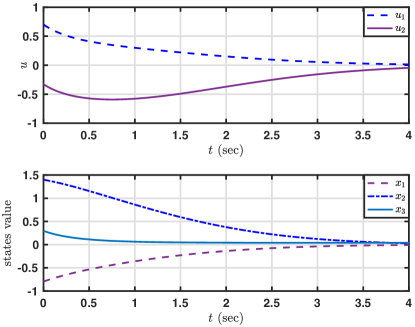
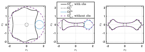
We take $[t_{0},T]=[0,4\ \text{sec}]$, $r_{T}(x)=x^{T}x-0.2^{2}$, $\epsilon=1\times 10^{-3}$, and impose bounds on control inputs $u_{1},u_{2}\in[-1,1]$. A closed-loop simulation with the resulting controller and initial condition $[-0.8,1.4,0.3]$ is shown in Figure 1. Figure 2 shows the slices of sets with $x_{3}=0$, $x_{2}=0$, and $x_{1}=0$, respectively. $\Omega_{t_{0},\gamma}^{V}$ is shown as the dashed curves and $\Omega_{0}^{r_{T}}$ is shown as the dash-dot curves.

Figure 1: Dubin’s car Simulations

5.1.1 Dubin’s Car with Obstacle

In addition to the terminal target set $\Omega_{0}^{r_{T}}$, suppose there is an unsafe region $\Omega_{0}^{obs}:=\{x\in\mathbb{R}^{3}|obs(x):=(x_{1}-1.5)^{2}+x_{2}^{2}+x_{3}^{2}-0.5^{2}\leq 0\}$. Thus the target tube is the intersection of the terminal target set $\Omega_{0}^{r_{T}}$ and the complement of $\Omega_{0}^{obs}$. Slices of the resulting $\Omega_{t_{0},\gamma}^{V}$ with the obstacle are shown as solid black curves in Figure 2.

Figure 2: Inner-approximated BRS for Dubin’s car example

5.2 Pendubot Example

Consider the following polynomial dynamics for a pendubot

$$\begin{bmatrix}\dot{x}_{1}\\ \dot{x}_{2}\\ \dot{x}_{3}\\ \dot{x}_{4}\end{bmatrix}=\begin{bmatrix}x_{2}\\ f_{2}(x_{1},x_{2},x_{3},x_{4})\\ x_{4}\\ f_{4}(x_{1},x_{2},x_{3},x_{4})\end{bmatrix}+\begin{bmatrix}0\\ g_{2}(x_{3})\\ 0\\ g_{4}(x_{3})\end{bmatrix}u,$$

with

$$f_{2} =-10.656x_{1}^{3}+11.531x_{1}^{2}x_{3}+7.885x_{1}x_{3}^{2}+0.797x_{2}^{2}x_{3}+0.841x_{2}x_{3}x_{4}+21.049x_{3}^{3}+$$

$$\quad\quad\quad 0.420x_{3}x_{4}^{2}+66.523x_{1}-24.511x_{3},$$

$$f_{4} =10.996x_{1}^{3}-48.915x_{1}^{2}x_{3}-6.404x_{1}x_{3}^{2}-2.396x_{2}^{2}x_{3}-1.594x_{2}x_{3}x_{4}-51.909x_{3}^{3}-$$

$$\quad\quad\quad 0.797x_{3}x_{4}^{2}-68.642x_{1}+103.978x_{3},$$

$$g_{2} =-10.096x_{3}^{2}+44.252,$$

$$g_{4} =37.802x_{3}^{2}-83.912,$$

which is obtained as a least-squares approximation of the full equations for $x_{1}\times x_{3}\in[-1,1]\times[-1,1]$.

Here $x_{1}$ and $x_{3}$ represent $\theta_{1}$ (rad) and $\theta_{2}$ (rad), which are angular positions of the first link and the second link (relative to the first link), respectively, and $x_{2}$ and $x_{4}$ are $\dot{\theta}_{1}$ (rad/s) and $\dot{\theta}_{2}$ (rad/s), which are corresponding angular velocities. Input $u$ (Nm) is the torque applied at the joint of first link and ground, but there is no torque applied at the joint of two links.

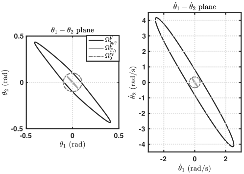
We take the time horizon $[0,4\ \text{sec}]$, $r_{T}(x)=x^{T}$ $diag(1/0.1^{2},$ $1/0.35^{2},$ $1/0.1^{2},$ $1/0.35^{2})x-1$, $\epsilon=1\times 10^{-4}$, and impose a bound on the control input $u\in[-1,1]$. Slices of sets shown on the left side of Figure 3 are plotted with $\dot{\theta}_{1}$ and $\dot{\theta}_{2}$ fixed at $0$. Slices of sets shown on the right side of Figure 3 are plotted with $\theta_{1}$ and $\theta_{2}$ fixed at $0$.

Figure 3: Inner-approximated BRS for the pendubot example

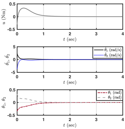
A simulation result with the initial condition [$-0.35$ rad; $2.6$ rad/s; $0.35$ rad; $-4$ rad/s], under the designed polynomial control law is shown in Figure 4.

Figure 4: Pendubot simulation results

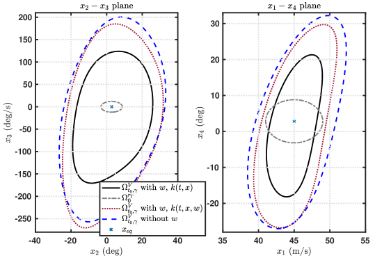
5.3 NASA’s Generic Transport Model (GTM) around straight and level flight condition with $\mathcal{L}_{2}$ Disturbance

The GTM is a remote-controlled 5.5% scale commercial aircraft [24]. From [25], its longitudinal dynamical model is

$$\dot{x}_{1}= \frac{1}{m}(-D-mg\sin(x_{4}-x_{2})+T_{x}\cos(x_{2})+T_{z}\sin(x_{2})),$$ (4)

$$\dot{x}_{2}= \frac{1}{mx_{1}}(-L+mg\cos(x_{4}-x_{2})-T_{x}\sin(x_{2})+T_{z}\cos(x_{2})+x_{3}),$$

$$\dot{x}_{3}= \frac{M+T_{m}}{I_{yy}},$$

$$\dot{x_{4}}= x_{3},$$

where $x_{1}$ to $x_{4}$ represent air speed (m/s), angle of attack (rad), pitch rate (rad/s) and pitch angle (rad), respectively. The control inputs are elevator deflection $u_{elev}$ (rad) and engine throttle $u_{th}$ (percent). The drag force $D$ (N), lift force $L$ (N), and aerodynamic pitching moment $M$ (N m) are given by $D=\bar{q}SC_{D}(x_{2},u_{elev},\hat{q})$, $L=\bar{q}SC_{L}(x_{2},u_{elev},\hat{q})$, and $M=\bar{q}S\bar{c}C_{m}(x_{2},u_{elev},\hat{q})$,where $\bar{q}:=\frac{1}{2}\rho x_{1}^{2}$ is the dynamic pressure (N/m²), $\hat{q}:=(\bar{c}/2x_{1})x_{3}$ is the normalized pitch rate (unitless), $S$ and $\bar{c}$ are the surface area and mean aerodynamic chord (both in m). $C_{D},C_{L},$ and $C_{m}$ are aerodynamic coefficients computed from look-up tables provided by NASA [26].

A 4-state, 2-input, degree-7 polynomial model is obtained in [26] by replacing all nonpolynomial terms in (4) with their polynomial approximations. The following straight and level trim-condition is computed for this model: $x_{1,t}=45$ m/s, $x_{2,t}=0.04924$ rad, $x_{3,t}=0$ rad/s, $x_{4,t}=0.04924$ rad, with $u_{elev,t}=0.04892$ rad, and $u_{th,t}=14.33\%$. A 4-state, degree-3, single-input polynomial longitudinal model is extracted from the 4-state, 2-input, degree-7 polynomial model by holding $u_{th}$ at its trim value, and retaining terms up to degree-3. This degree-3 polynomial model is used for the following synthesis.

The disturbance $w$ is the perturbation to the angle of attack caused by a change in wind direction, i.e. the force generated on the aircraft is due to wind coming at an angle $(x_{2}+w)$. Denote the nominal GTM system as $F(x,u):=f(x)+g(x)u$; then the disturbed system is given as

$$\dot{x} =F(x,u)+\frac{dF(x,u)}{dx_{2}}w$$

$$=f(x)+\frac{f(x)}{dx_{2}}w+(g(x)+\frac{dg(x)}{dx_{2}}w)u.$$ (5)

The disturbance $w$ is assumed to have both $\mathcal{L}_{2}$ and $\mathcal{L}_{\infty}$ bounds: $R:=0.1$ rad, $\int_{0}^{t}w^{T}(\tau)w(\tau)d\tau\leq R^{2}q(t):=R^{2}t^{2}/T^{2}$, for all $t\in[0,3\ \text{sec}]$ and $\left\lVert w(t)\right\rVert_{2}\leq\overline{w}:=0.141$ rad. Set the time horizon [$0,3$ sec], $\epsilon=1\times 10^{-4}$, the control constraint $u_{elev}\in[-10^{\circ},10^{\circ}]$, and $r_{T}(x)=(x-x_{eq})^{T}diag(1/4^{2},1/(\pi/30)^{2},1/(\pi/15)^{2},1/(\pi/30)^{2})(x-x_{eq})-1$, where the equilibrium point $x_{eq}:=[x_{1,t},x_{2,t},x_{3,t},x_{4,t}]^{T}$.

In this section, we inner-approximate the BRS for three cases: without disturbance $w$ and $k$ is a function of $t,x$; with disturbance $w$ and $k$ is allowed to be a function of $t,x,w$; with disturbance $w$ but $k$ is a function of only $t,x$. Curves shown on the left side of Figure 5 are slices of sets with $x_{1}=x_{1,t}$ and $x_{4}=x_{4,t}$; curves shown on the right side are slices of sets with $x_{2}=x_{2,t}$ and $x_{3}=x_{3,t}$. Notice that the volume of inner-approximations of BRS for the two cases with disturbance are smaller than without disturbance. Moreover, for the two cases with disturbance, the volume of inner-approximations for the case using $k(t,x)$ is smaller than the case using $k(t,x,w)$.

Figure 5: Inner-approximated BRS for GTM

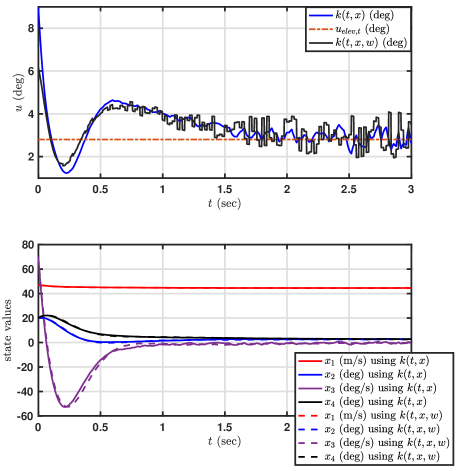
The simulation results of the polynomial model of GTM with the initial condition [$47$ m/s; $20$ rad; $70$ rad/s; $20$ rad] and a disturbance signal $w(t)=\frac{\sqrt{2t}R}{T}\eta(t)$, using both $k(t,x)$ and $k(t,x,w)$ are shown in Figure 6, where the value of $\eta(t)$ is updated by the number drawn from the uniform distribution on the interval $(-1,1)$ at 50 Hz, and holds at the updated value until the next update. As we can see in the figure, the trajectory for pitch rate $x_{3}$ with $k(t,x,w)$ reaches trim value faster than the one with $k(t,x)$, and the former is much smoother.

Figure 6: Simulations of GTM with disturbances $w$

5.4 Pursuer-evader Game

Consider the reach-avoid example from [3]. Assume that there are two players, the evader and the pursuer. Fix the evader at the origin and facing along the positive $x_{1}$ axis, so that the pursuer’s relative location and heading are described by

$$\begin{bmatrix}\dot{x}_{1}\\ \dot{x}_{2}\\ \dot{x}_{3}\end{bmatrix}=\begin{bmatrix}-v_{e}+v_{p}\cos(x_{3})+u_{e}x_{2}\\ v_{p}\sin(x_{3})-u_{e}x_{1}\\ u_{p}-u_{e}\end{bmatrix},$$ (6)

where $x_{1},x_{2},x_{3}$ represent relative $x,y$ positions and heading angle; $u_{e}$ and $u_{p}$ are angular velocity inputs from the evader and pursuer; $v_{e}$ and $v_{p}$ are velocities of the evader and pursuer.

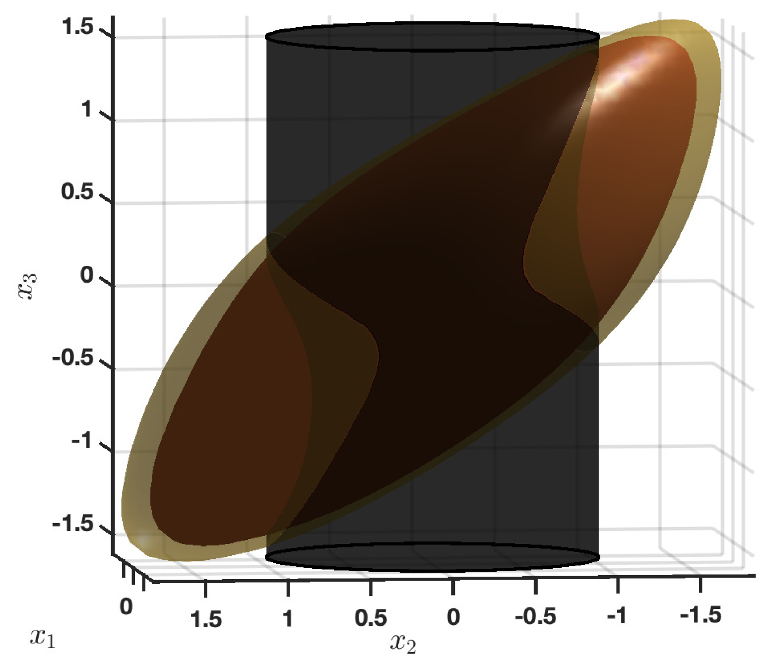
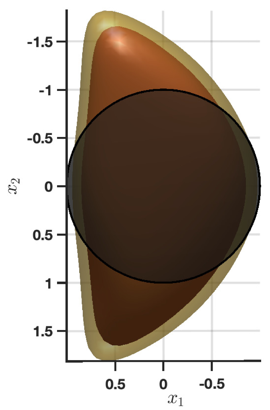
Set the time horizon $[0,2.6\ \text{sec}]$, and $r_{T}(x)=x^{T}x-1$. Velocities of two players are constant: $v_{e}=v_{p}=1$, control input is $u_{p}(t)\in[-1,1]$. The goal for the pursuer is to find a robust control law for $u_{p}$ and an inner-approximated BRS, so that no matter how the evader chooses its control input at each time instance, all the trajectories for system (6) from the inner-approximated BRS will always be driven to the target set $\Omega_{0}^{r_{T}}$. This reachability problem is posed as a dynamic game in [3], whereas in this paper, the control input $u_{e}$ from the evader is regarded as the uncertain parameter with a given $\mathcal{L}_{\infty}$ bound: $u_{e}(t)\in[-0.5,0.5]$. In this example, $\cos(x_{3})$ is approximated by $(-0.4298x_{3}^{2}+1)$, and $\sin(x_{3})$ is approximated by $(-0.1511x_{3}^{3}+x_{3})$, which are obtained by least square regression for $x_{3}\in[-\frac{\pi}{2},\frac{\pi}{2}]$. Polynomial dynamics of (6) can be obtained by replacing $\cos(x_{3})$ by $(-0.4298x_{3}^{2}+1+\delta_{\cos})$, where accounting for the error between $\cos(x_{3})$ and its polynomial approximation yields $\delta_{\cos}(t)\in[-0.05,0.05]$ for $x_{3}\in[-\frac{\pi}{2},\frac{\pi}{2}]$. The error between $\sin(x_{3})$ and its polynomial approximation is very small and it is neglected. Setting $\delta_{\cos}(t)=0$, neglects the $\cos(x_{3})$ error as well.

The results are computed for the two cases: $\delta_{\cos}(t)\in[-0.05,0.05]$ or $\delta_{\cos}(t)=0$. In Figure 7, computed inner-approximations are shown with solid red and translucent brown, respectively. The computed storage function of the former case is used as the initial iterate $V^{0}$ for the latter. The target set is shown with the transparent black cylinder. We can see that when $\delta_{\cos}(t)\in[-0.05,0.05]$, the BRS inner-approximation is smaller than when $\delta_{\cos}(t)=0$, but robust against the error resulting from polynomial modelling.

(a) 3D view

(b) Top view

Figure 7: Inner-approximated BRS for the pursuer-evader game

6 Conclusions

We proposed a method for synthesizing controllers for nonlinear systems with polynomial vector fields. The synthesis process yields a state-feedback control law, and a reachability storage function that characterizes an inner-approximation to the BRS for a given target tube. An iterative algorithm to construct them is derived based on SOS programming and the S-procedure. The synthesis framework is also extended to uncertain systems with $\mathcal{L}_{\infty}$ parametric uncertainties and $\mathcal{L}_{2}$ disturbances. This method is applied to several practical robotics and aircraft models. Currently, the computational complexity of our method limits it to systems of modest size, with fewer than ten state variables.

References

- [1] A. Majumdar, A. A. Ahmadi, and R. Tedrake, “Control design along trajectories with sums of squares programming,” in Proceedings of International Conference on Robotics and Automation, 2013, pp. 4054–4061.
- [2] A. Majumdar and R. Tedrake, “Funnel libraries for real-time robust feedback motion planning,” The International Journal of Robotics Research, vol. 36, no. 8, pp. 947–982, 2017.
- [3] I. M. Mitchell, A. M. Bayen, and C. J. Tomlin, “A time-dependent Hamilton–Jacobi formulation of reachable sets for continuous dynamic games,” IEEE Transactions on Automatic Control, vol. 50, pp. 947 – 957, 2005.
- [4] D. Henrion and M. Korda, “Convex computation of the region of attraction of polynomial control systems,” IEEE Transactions on Automatic Control, vol. 59, pp. 297–312, 2014.
- [5] A. Majumdar, R. Vasudevan, M. M. Tobenkin, and R. Tedrake, “Convex optimization of nonlinear feedback controllers via occupation measures,” The International Journal of Robotics Research, vol. 33, pp. 1209–1230, 2014.
- [6] P. Parrilo, “Structured semidefinite programs and semialgebraic geometry methods in robustness and optimization,” PhD thesis, California Institute of Technology, 2000.
- [7] U. Topcu, “Quantitative local analysis of nonlinear systems,” PhD thesis, University of California, Berkeley, 2008.
- [8] W. Tan and A. Packard, “Stability region analysis using polynomial and composite polynomial Lyapunov functions and sum-of-squares programming,” IEEE Transactions on Automatic Control, vol. 53, p. 565, 2008.
- [9] G. Chesi, A. Garulli, A. Tesi, and A. Vicino, “LMI-based computation of optimal quadratic Lyapunov functions for odd polynomial systems,” International Journal of Robust and Nonlinear Control, vol. 15, no. 1, pp. 35–49, 2005.
- [10] B. Tibken and Youping Fan, “Computing the domain of attraction for polynomial systems via BMI optimization method,” in 2006 American Control Conference, Minneapolis, MN, June 2006, pp. 117–122.
- [11] A. Iannelli, P. Seiler, and A. Marcos, “Region of attraction analysis with integral quadratic constraints,” submitted to Automatica.
- [12] Z. Jarvis-Wloszek, R. Feeley, W. Tan, K. Sun, and A. Packard, “Controls applications of sum of squares programming,” in Positive Polynomials in Control. Springer, Berlin, Heidelberg, 2005, vol. 312.
- [13] H. Yin, A. Packard, M. Arcak, and P. Seiler, “Finite horizon backward reachability analysis and control synthesis for uncertain nonlinear systems,” to appear in 2019 American Control Conference.
- [14] ——, “Reachability analysis using dissipation inequalities for nonlinear dynamical systems,” arXiv preprint, aug 2018, arXiv:1808.02585.
- [15] U. Topcu and A. Packard, “Linearized analysis versus optimization-based nonlinear analysis for nonlinear systems,” in Proceedings of 2009 American Control Conference, St. Louis, MO, USA, 2009.
- [16] E. Summers, A. Chakraborty, W. Tan, U. Topcu, P. Seiler, G. Balas, and A. Packard, “Quantitative local -gain and reachability analysis for nonlinear systems,” International Journal of Robust and Nonlinear Control, vol. 23, pp. 1115–1135, 2013.
- [17] P. Seiler and G. Balas, “Quasiconvex sum-of-squares programming,” in Proceedings of 49th IEEE Conference on Decision and Control, Atlanta, GA, USA, 2010, pp. 3337–3342.
- [18] S. Boyd and L. E. Ghaoui, “Method of centers for minimizing generalized eigenvalues,” Linear Algebra and its Applications, vol. 188-189, pp. 63–111, 1993.
- [19] S. Boyd and L. Vandenberghe, Convex Optimization. Cambridge University Press, 2004.
- [20] P. Seiler, “SOSOPT: A toolbox for polynomial optimization,” ArXiv e-prints, Aug 2013, arXiv:1308.1889.
- [21] MOSEK ApS, “The MOSEK optimization toolbox for MATLAB manual. Version 8.1.” 2017, http://docs.mosek.com/8.1/toolbox/index.html.
- [22] L. Dubins, “On curves of minimal length with a constraint on average curvature, and with prescribed initial and terminal positions and tangents,” American Journal of Mathematics, vol. 79, no. 3, pp. 497–516, 1957.
- [23] D. DeVon and T. Bretl, “Kinematic and dynamic control of a wheeled mobile robot,” in IEEE/RSJ International Conference on Intelligent Robots and Systems. IEEE, 2007, pp. 4065–4070.
- [24] A. M. Murch and J. V. Foster, “Recent NASA research on aerodynamic modeling of poststall and spin dynamics of large transport airplanes,” in In 45th AIAA Aerospace Sciences Meeting and Exhibit, Reno, Nevada, 2007.
- [25] B. L. Stevens and F. L. Lewis, Aircraft Control and Simulation. Hoboken, NJ: John Wiley & Sons, 1992.
- [26] A. Chakraborty, P. Seiler, and G. J. Balas, “Nonlinear region of attraction analysis for flight control verification and validation,” Control Engineering Practice, vol. 19, no. 4, pp. 335–345, 2011.