Convergence Analysis of a Collapsed Gibbs Sampler for Bayesian Vector Autoregressions

Abstract

We study the convergence properties of a collapsed Gibbs sampler for Bayesian vector autoregressions with predictors, or exogenous variables. The Markov chain generated by our algorithm is shown to be geometrically ergodic regardless of whether the number of observations in the underlying vector autoregression is small or large in comparison to the order and dimension of it. In a convergence complexity analysis, we also give conditions for when the geometric ergodicity is asymptotically stable as the number of observations tends to infinity. Specifically, the geometric convergence rate is shown to be bounded away from unity asymptotically, either almost surely or with probability tending to one, depending on what is assumed about the data generating process. This result is one of the first of its kind for practically relevant Markov chain Monte Carlo algorithms. Our convergence results hold under close to arbitrary model misspecification.

1 Introduction

Markov chain Monte Carlo (MCMC) is often used to explore the posterior distribution of a vector of parameters $\theta$ given data $\mathcal{D}$. To ensure the reliability of an analysis using MCMC it is essential to understand the convergence properties of the chain in use [6, 7, 9, 10, 20, 26, 48] and, accordingly, there are numerous articles establishing such properties for different MCMC algorithms [e.g. 1, 2, 13, 15, 17, 21, 32, 38, 46]. It has been common in this literature to treat the data $\mathcal{D}$ as fixed, or realized. Thus, the model for how the data are generated has typically been important only insofar as it determines the likelihood function based on an arbitrary realization—the stochastic properties of the data prescribed by that model have not been emphasized. This is natural since the target distribution, i.e. the posterior distribution, treats the data as fixed. On the other hand, due to the rapid growth of data available in applications, it is also desirable to understand how performance is affected as the number of observations increases. When this happens, the data are more naturally thought of as stochastic; each time the sample size increases by one, the additional observation is randomly generated. The study of how convergence properties of MCMC algorithms are affected by changes in the data is known as convergence complexity analysis [35] and it has attracted increasing attention recently [16, 32, 34, 49, 50].

Accounting for randomness in the data and letting the sample size grow leads to a more complicated analysis than when the data are fixed. In fact, to date, convergence complexity analysis has only been successfully carried out for a few, maybe even one [32], practically relevant MCMC algorithms, by which we mean MCMC algoritms for settings where one could not easily sample by less complicated methods. We study a MCMC algorithm for a fundamental model in time series analysis: a Bayesian vector autoregression with predictors (VARX). Briefly, the VARX we consider assumes that $Y_{t}\in\mathbb{R}^{r}$ and $X_{t}\in\mathbb{R}^{p}$ satisfy, for $t=1,\dots,n$,

$$Y_{t}=\sum_{i=1}^{q}\mathcal{A}_{i}^{\mathsf{T}}Y_{t-i}+\mathcal{B}^{\mathsf{T}}X_{t}+U_{t}$$ (1)

with $U_{1},\dots,U_{n}$ independent and multivariate normally distributed with mean zero and common covariance matrix $\Sigma\in\mathbb{S}^{r}_{++}$, the set of $r\times r$ symmetric and positive definite (SPD) matrices, $\mathcal{A}_{i}\in\mathbb{R}^{r\times r}$, $i=1,\dots,q$, and $\mathcal{B}\in\mathbb{R}^{p\times r}$. As we will see, the likelihood for the VARX is closely related to that of a multivariate linear regression and, consequently, our results apply also to that model. Moreover, (1) simplifies to a multivariate linear regression if $\mathcal{A}_{i}=0$ for all $i$. We focus on the VARX because it motivates our study and, in particular, our choice of priors. More details on the model specification, priors, and resulting posterior distributions are given in Section 2.

The target distribution of our algorithm is the posterior distribution of $\theta=(\mathcal{A}_{1},\dots,\mathcal{A}_{q},\mathcal{B},\Sigma)$ given $\mathcal{D}=\{(Y_{1},X_{1}),\dots,(Y_{n},X_{n})\}$. We will consider both fixed and growing data and refer to the two settings as the small-$n$ and large-$n$ setting, respectively. By $n$ being small we mean that it is fixed and possibly small in comparison to $r$ and $q$, but $n>p$ throughout. Many large VARs in the literature [3, 11, 24] are covered by this setting. By $n$ being large we mean that it is increasing and that the data are stochastic.

The algorithm we consider is a collapsed Gibbs sampler that simplifies to a commonly considered (non-collapsed) Gibbs sampler when there are no predictors in the model; that is, when $\mathcal{B}\equiv 0$ in (1). To discuss our results, we require some more notation. Let $F(\cdot|\mathcal{D})$ denote the VARX posterior distribution having density $f(\theta|\mathcal{D})$ with support on $\Theta\subseteq\mathbb{R}^{d}$ for some $d\geq 1$ and let $K^{h}$ ($K\equiv K^{1}$) be the $h$-step transition kernel for a Markov chain with state space $\Theta$, started at a point $\theta\in\Theta$. We assume throughout that all discussed Markov chains are irreducible, aperiodic, and Harris recurrent [31], and that sets on which measures are defined are equipped with their Borel $\sigma$-algebra. Our analysis is focused on convergence rates in total variation distance, by which we mean the rate at which $\|K^{h}(\theta,\cdot)-F(\cdot|\mathcal{D})\|_{TV}$ approaches zero as $h$ tends to infinity, where $\|\cdot\|_{TV}$ denotes the total variation norm. If this convergence happens at a geometric (or exponential) rate, meaning there exist a $\rho\in[0,1)$ and an $M:\Theta\to[0,\infty)$ such that for every $\theta\in\Theta$ and $h\in\{1,2,\dots\}$

$$\|K^{h}(\theta,\cdot)-F(\cdot|\mathcal{D})\|_{TV}\leq M(\theta)\rho^{h},$$ (2)

then the Markov chain, or the kernel $K$, is said to be geometrically ergodic. The geometric convergence rate $\rho^{\star}$ is the infimum of the set of $\rho\in[0,1]$ such that (2) holds [32]. Since all probability measures have unit total variation norm, $\rho^{\star}$ is always in $[0,1]$, and $K$ is geometrically ergodic if and only if $\rho^{\star}<1$. A substantial part of the literature on convergence of MCMC algorithms is centered around geometric ergodicity, for good reasons: under moment conditions, a central limit theorem (CLT) holds for functionals of geometrically ergodic Markov chains [5, 18] and the variance in the asymptotic distribution given by that CLT can be consistently estimated [8, 19, 47], allowing principled methods for ensuring reliability of the results [39, 48]. Our main result in the small-$n$ setting gives conditions that ensure $\rho^{\star}<1$ when the data are fixed and $K$ is the kernel corresponding to the algorithm we consider.

Notice that, although it is suppressed in the notation, $K$, $M$, $\rho$, and, hence, $\rho^{\star}$ typically depend on $\mathcal{D}$. In the large-$n$ setting, we are no longer considering a single dataset, but a sequence of datasets $\{\mathcal{D}_{n}\}:=\{\mathcal{D}_{1},\mathcal{D}_{2},\dots\}$, where $\mathcal{D}_{n}$ here denotes a dataset with $n$ observations. Consequently, for every $n$ there is a posterior distribution $F(\cdot|\mathcal{D}_{n})$ and a Markov chain with kernel $K_{n}$ that is used to explore it. To each kernel $K_{n}$ there also corresponds a geometric convergence rate $\rho^{\star}_{n}$. Since $\rho^{\star}_{n}$ depends on $\mathcal{D}_{n}$, the sequence $\{\rho^{\star}_{n}\}$ is now one of random variables, ignoring possible issues with measurability. If the convergence rate $\rho_{n}^{\star}$ tends to one in probability or almost surely as $n\to\infty$, we say that the convergence rate is unstable; in practice, we expect an algorithm that generates a chain with geometric convergence rate tending to one to be less reliable when applied to large datasets. Thus, we are interested in bounding $\{\rho^{\star}_{n}\}$ away from unity asymptotically, in either one of two senses: first, if there exists a sequence of random variables $\{\bar{\rho}_{n}\}$ such that $\rho^{\star}_{n}\leq\bar{\rho}_{n}$ for every $n$ and $\limsup_{n\to\infty}\bar{\rho}_{n}<1$ almost surely, then we say that $\{K_{n}\}$ is asymptotically geometrically ergodic almost surely, or the geometric ergodicity is asymptotically stable almost surely. Secondly, if instead of the upper limit being less than unity almost surely it holds that $\lim_{n\to\infty}\mathsf{P}(\bar{\rho}_{n}<1)=1$, then we say that $\{K_{n}\}$ is asymptotically geometrically ergodic in probability, or that the geometric ergodicity is asymptotically stable in probability. In the large-$n$ setting, we give conditions for asymptotically stable geometric ergodicity, in both of the two senses, of the Markov chain generated by our algorithm. An intuitive, albeit somewhat loose, interpretation of our main results is that the geometric ergodicity is asymptotically stable if the sample covariance matrix $n^{-1}\sum_{t=1}^{n}[Y_{t}^{\mathsf{T}},\dots,Y_{t-q}^{\mathsf{T}},X_{t}^{\mathsf{T}}][Y_{t}^{\mathsf{T}},\dots,Y_{t-q}^{\mathsf{T}},X_{t}^{\mathsf{T}}]^{\mathsf{T}}$ tends to some positive definite limit. In particular, as long as this holds, the geometric ergodicity of the Markov chain we study is asymptotically stable under arbitrary model misspecification. Our small- and large-$n$ results are complementary: the small-$n$ results establish geometric ergodicity for fixed $n$ but do not ensure asymptotic geometric ergodicity, while the laarge-$n$ results give asymptotic geometric ergodicity but do not imply geometric ergodicity for fixed $n$.

The rest of the paper is organized as follows. We begin in Section 2 by completing the specification of the model and priors. Because some of the priors may be improper we derive conditions which guarantee the posterior exists and is proper. In Section 3 we develop a collapsed Gibbs sampler for exploring the posterior. Conditions for geometric ergodicity for small $n$ are presented in Section 4 and conditions for asymptotically stable geometric ergodicity are given in Section 5. Some concluding remarks are given in Section 6.

2 Bayesian vector autoregression with predictors

Recall the definition of the VARX in (1). To complete the specification, we assume that the starting point $(Y_{-q+1},\dots,Y_{0})$ is non-stochastic and known and that the predictors are strongly exogenous. By the latter we mean that $\{X_{t}\}$ is independent of $\{U_{t}\}$ and has a distribution that does not depend on the model parameters. With these assumptions the following lemma is straightforward. Its proof is provided in Appendix B for completeness. Let $Y=[Y_{1},\dots,Y_{n}]^{\mathsf{T}}\in\mathbb{R}^{n\times r}$, $X=[X_{1},\dots,X_{n}]^{\mathsf{T}}\in\mathbb{R}^{n\times p}$, $Z_{t}=[Y_{t-1}^{\mathsf{T}},\dots,Y_{t-q}^{\mathsf{T}}]^{\mathsf{T}}\in\mathbb{R}^{qr}$, $t=1,\dots,n$, and $Z=[Z_{1},\dots,Z_{n}]^{\mathsf{T}}\in\mathbb{R}^{n\times qr}$. Let also $\mathcal{A}=[\mathcal{A}_{1}^{\mathsf{T}},\dots,\mathcal{A}_{q}^{\mathsf{T}}]^{\mathsf{T}}\in\mathbb{R}^{qr\times r}$ and $\alpha=\operatorname{vec}(\mathcal{A})$, where $\operatorname{vec}(\cdot)$ is the vectorization operator, stacking the columns of its matrix argument.

Lemma 2.1.

The joint density for $n$ observations in the VARX is $f(Y,X\mid\mathcal{A},\mathcal{B},\Sigma)=f(X)f(Y\mid X,\mathcal{A},\mathcal{B},\Sigma)$ with $f(Y\mid X,\mathcal{A},\mathcal{B},\Sigma)$ given by

$$\begin{split}(2\pi)^{-nr/2}|\Sigma|^{-n/2}\operatorname{etr}\left[-\frac{1}{2}\Sigma^{-1}(Y-Z\mathcal{A}-X\mathcal{B})^{\mathsf{T}}(Y-Z\mathcal{A}-X\mathcal{B})\right]\end{split},$$

where $\operatorname{etr}(\cdot)=\exp(\operatorname{tr}(\cdot))$.

For fixed data, $f(Y\mid X,\mathcal{A},\mathcal{B},\Sigma)$ is the same as for a multivariate linear regression with partitioned design matrix $[Z,X]\in\mathbb{R}^{n\times(qr+p)}$ and coefficient matrix $[\mathcal{A}^{\mathsf{T}},\mathcal{B}^{\mathsf{T}}]^{\mathsf{T}}$. However, our choice of priors is guided by the vector autoregression. Let $\mathbb{S}^{r}_{+}$ denote the set of $r\times r$ symmetric positive semi-definite (SPSD) matrices and, to define priors, let $m\in\mathbb{R}^{qr^{2}}$, $C\in\mathbb{S}^{qr^{2}}_{+}$, $D\in\mathbb{S}^{r}_{+}$, and $a\geq 0$ be hyperparameters. Our prior on $\theta=(\alpha,\mathcal{B},\Sigma)\in\Theta=\mathbb{R}^{qr^{2}}\times\mathbb{R}^{p\times r}\times\mathbb{S}^{r}_{++}$ is of the form $f(\theta)=f(\alpha)f(\mathcal{B})f(\Sigma)$, with

$$f(\alpha) \propto\exp\left(-\frac{1}{2}[\alpha-m]^{\mathsf{T}}C[\alpha-m]\right),$$

$$f(\mathcal{B}) \propto 1,$$

and

$$f(\Sigma)\propto|\Sigma|^{-a/2}\operatorname{etr}\left(-\frac{1}{2}D\Sigma^{-1}\right),$$

where $|\cdot|$ means the determinant when applied to matrices. The flat prior on $\mathcal{B}$ is standard in multivariate scale and location problems, including in particular the multivariate regression model. The priors on $\alpha$ and $\Sigma$ are common in macroeconomics [23] and the prior on $\Sigma$ includes the inverse Wishart ($D\in\mathbb{S}^{r}_{++},a>2r$) and Jeffreys prior ($D=0,a=r+1$) as special cases. In other work on similar models it is often assumed that $[Z,X]$ has full rank or that the prior for $[\mathcal{A}^{\mathsf{T}},\mathcal{B}^{\mathsf{T}}]^{\mathsf{T}}$ is proper [1, 2, 11, 13, 25, 44]. Treating $\mathcal{A}$ and $\mathcal{B}$ differently is appealing in the current setting: it adheres to the common practice of using flat priors for regression coefficients such as $\mathcal{B}$, while $m$ and $C$ can be chosen to reflect the fact that many commonly studied time series are known to be near non-stationary in the unit root sense. In particular, with economic and financial data it is often reasonable to expect the diagonal elements of $\mathcal{A}_{1}$ to be near one. For a more thorough discussion of popular priors in Bayesian VARs we refer the reader to Karlsson [23].

The following result gives two different sets of conditions that lead to a proper posterior. Though we focus on proper normal or flat priors for $\alpha$ in the rest of the paper, it may be relevant for other work to note that the proposition holds for any prior $f(\alpha)$ satisfying the conditions. For example, $f(\alpha)$ could be truncated to impose stability of the VARX, which if $q=1$ corresponds to a prior with support only on $\alpha$ for which the spectral norm of $\mathcal{A}$ is less than one [see e.g. 28, for definitions].

Proposition 2.2.

If either

1. $D\in\mathbb{S}^{r}_{++}$, $X$ has full column rank, $n+a>2r+p$, and $f(\alpha)$ is proper; or

2. $[Y,Z,X]\in\mathbb{R}^{n\times(r+qr+p)}$ has full column rank, $n+a>(2+q)r+p$, and $f(\alpha)$ is bounded,

then the posterior distribution is proper; if, in addition, $f(\alpha)\propto\exp(-[\alpha-m]^{\mathsf{T}}C[\alpha-m]/2)$, then with $S=n^{-1}(Y-Z\mathcal{A}-X\mathcal{B})^{\mathsf{T}}(Y-Z\mathcal{A}-X\mathcal{B})$, the posterior density is characterized by

$$f(\mathcal{A},\mathcal{B},\Sigma\mid Y,X)\propto|\Sigma|^{-\frac{n+a}{2}}\operatorname{etr}\left(-\frac{1}{2}\Sigma^{-1}[D+nS]-\frac{1}{2}(\alpha-m)^{\mathsf{T}}C(\alpha-m)\right).$$ (3)

Proof.

Appendix B. ∎

The first set of conditions is relevant to the small $n$-setting. It implies that if the prior on $\Sigma$ is a proper inverse Wishart density, so that $a>2r$ and $D\in\mathbb{S}^{r}_{++}$, then the posterior is proper if $f(\alpha)$ is proper and $X$ has full column rank. In particular, $r$ or $q$ can be arbitrarily large in comparison to $n$. Thus, this setting is compatible with large VARs [3, 11, 24]. The second set of conditions allows for the use of improper priors also on $\alpha$ and $\Sigma$ when $n$ is large in comparison to all of $p$, $q$, and $r$. The full column rank of $[Y,Z,X]$ is natural in large-$n$ settings. In practice, one expects it to hold unless the squares regression of $Y$ on $Z$ and $X$ gives residuals that are identically zero.

The literature on convergence properties of MCMC algorithms for Bayesian VAR(X)s is limited. An MCMC algorithm for a multivariate linear regression model has been proposed and its convergence rate in the small-$n$ setting studied [13]. By the preceding discussion, this includes the VARX as a special case, however, the (improper) prior used is $f(\theta)\propto|\Sigma|^{-a}$ which is not compatible with the large VARXs we allow for in the small-$n$ setting. A two-component ($\mathcal{A}$ and $\Sigma$) Gibbs sampler for Bayesian vector autoregressions without predictors has been proposed [22], but the analysis of it is simulation-based and as such does not provide any theoretical guarantees. Our results address this since, as we will discuss in more detail below, the algorithm we consider simplifies to this Gibbs sampler when there are no predictors.

3 A collapsed Gibbs sampler

If the precision matrix in the prior on $f(\alpha)$, $C$, is a matrix of zeros, then the VARX posterior is a normal-(inverse) Wishart for which MCMC is unnecessary. However, when $C\in\mathbb{S}^{qr^{2}}_{++}$ the posterior is analytically intractable and there are many potentially useful MCMC algorithms. For example, the full conditional distributions have familiar forms so it is straightforward to implement a three-component Gibbs sampler. Another sensible option is to group $\mathcal{A}$ and $\mathcal{B}$ and update them together. Here, we will instead make use of the particular structure the partitioned matrix $[Z,X]$ offers and devise a collapsed Gibbs sampler [27]; that is, a Gibbs sampler where some updates are not using full conditional distributions, but conditional distributions with one or more components integrated out. As we will see, the structure of the collapsed sampler, and in particular relations between the convergence rates of marginal chains and the full chain, is instrumental to our development. For a discussion more generally of how operator norms of collapsed and non-Collapsed Gibbs samplers compare we refer the reader to [27].

For the case where the precision matrix $C$ in the prior on $\alpha$ is positive definite and $\mathcal{B}\equiv 0$, so that the predictor matrix $X$ plays no role in the model, a two-component Gibbs sampler has been proposed [23]. We will show that the algorithm we study includes this Gibbs sampler as a special case, with minor modifications, and as a consequence our results apply almost verbatim to that sampler. A formal description of one iteration of the collapsed Gibbs sampler is given in Algorithm 1.

Algorithm 1 Collapsed Gibbs sampler

1:Input: Current value $(\alpha^{h},\mathcal{B}^{h},\Sigma^{h})$

2:Draw $\Sigma^{h+1}$ from the distribution of $\Sigma\mid\alpha^{h},Y,X$

3:Draw $\alpha^{h+1}$ from the distribution of $\alpha\mid\Sigma^{h+1},Y,X$

4:Draw $\mathcal{B}^{h+1}$ from the distribution of $\mathcal{B}\mid\alpha^{h+1},\Sigma^{h+1},Y,X$

5:Set $h=h+1$

We next give the conditional distributions necessary for its implementation. Let $\mathcal{M}(M,U,V)$ denote the matrix normal distribution with mean $M$ and scale matrices $U$ and $V$, that is, the distribution of a matrix whose vectorization is multivariate normal with mean $\operatorname{vec}(M)$ and covariance matrix $V\otimes U$, where $\otimes$ is the Kronecker product. Let also $\mathcal{W}^{-1}(U,c)$ denote the inverse Wishart distribution with scale matrix $U$ and $c$ degrees of freedom. For any real matrix $M$, define $P_{M}$ to be the projection onto its column space and $Q_{M}$ the projection onto the orthogonal complement of its column space. Finally, define $B=B(\Sigma)=C+\Sigma^{-1}\otimes Z^{\mathsf{T}}Q_{X}Z$ and $u=u(\Sigma)=B^{-1}[Cm+(\Sigma^{-1}\otimes Z^{\mathsf{T}}Q_{X})\operatorname{vec}(Q_{X}Y)]$.

Lemma 3.1.

If one of the two sets of conditions in Proposition 2.2 holds, then

$$\Sigma\mid\mathcal{A},Y,X\sim\mathcal{W}^{-1}\left(D+(Y-Z\mathcal{A})^{\mathsf{T}}Q_{X}(Y-Z\mathcal{A}),n+a-p-r-1\right),$$

$$\alpha\mid\Sigma,Y,X\sim\mathcal{N}(u,B^{-1})\text{, and }$$

$$\mathcal{B}\mid\mathcal{A},\Sigma,Y,X\sim\mathcal{M}\left([X^{\mathsf{T}}X]^{-1}X^{\mathsf{T}}(Y-Z\mathcal{A}),[X^{\mathsf{T}}X]^{-1},\Sigma\right).$$

Proof.

Appendix B. ∎

The collapsed Gibbs sampler in Algorithm 1 simulates a realization from a Markov chain having one-step transition kernel $K_{C}(\theta^{\prime},A)$ defined, for any measurable $A\subseteq\Theta=\mathbb{R}^{qr^{2}}\times\mathbb{R}^{p\times r}\times\mathbb{S}^{r}_{++}$, by

$$\iiint I_{A}(\alpha,\mathcal{B},\Sigma)f(\Sigma\mid\alpha^{\prime},Y,X)f(\alpha\mid\Sigma,Y,X)f(\mathcal{B}\mid\alpha,\Sigma,Y,X)\,\mathrm{d}\Sigma\,\mathrm{d}\alpha\,\mathrm{d}\mathcal{B},$$

where the subscript $C$ is short for collapsed. However, instead of working directly with $K_{C}$ we will use its structure to reduce the problem in a convenient way. Consider the sequence $\{(\alpha^{h},\Sigma^{h})\}$, $h=1,2,\dots$, obtained by ignoring the component for $\mathcal{B}$ in Algorithm 1. The sequence $\{(\alpha^{h},\Sigma^{h})\}$ is essentially generated by a two-component Gibbs sampler. More precisely, if $Q_{X}$ is replaced by the $n\times n$ identity $I_{n}$ in the conditional distributions of $\Sigma$ and $\alpha$ used in Algorithm 1, then the algorithm defined by steps 1, 2, 3, and 5 is a two-component Gibbs sampler exploring the posterior $f(\alpha,\Sigma\mid Y)$ for the model that takes $\mathcal{B}\equiv 0$ in (1). The transition kernel for $\{(\alpha^{h},\Sigma^{h})\}$ is, for any measurable $A\subseteq\mathbb{R}^{qr^{2}}\times\mathbb{S}^{r}_{++}$,

$$K_{G}((\alpha^{\prime},\Sigma^{\prime}),A)=\iint I_{A}(\alpha,\Sigma)f(\alpha\mid\Sigma,Y,X)f(\Sigma\mid\alpha^{\prime},Y,X)\,\mathrm{d}\alpha\,\mathrm{d}\Sigma.$$

A routine calculation shows that since $K_{G}$, by construction, has invariant distribution $F_{\mathcal{A},\Sigma}(\cdot\mid Y,X)$, then $K_{C}$ has the VARX posterior $F(\cdot|Y,X)$ as its invariant distribution.

The sequences $\{\alpha^{h}\}$ and $\{\Sigma^{h}\}$ are also Markov chains. The transition kernel for the $\{\alpha^{h}\}$ sequence is, for any measurable $A\subseteq\mathbb{R}^{qr^{2}}$,

$$K_{\mathcal{A}}(\alpha^{\prime},A)=\iint I_{A}(\alpha)f(\alpha\mid\Sigma,Y,X)f(\Sigma\mid\alpha^{\prime},Y,X)\,\mathrm{d}\Sigma\,\mathrm{d}\alpha.$$ (4)

The transition kernel, $K_{\Sigma}$, for the $\{\Sigma^{h}\}$ sequence is constructed similarly. The kernel $K_{\mathcal{A}}$ satisfies detailed balance with respect to the posterior marginal $F_{\mathcal{A}}(\cdot\mid Y,X)$ and similarly for $K_{\Sigma}$ and hence each has the respective posterior marginal as its invariant distribution. However, the kernels $K_{C}$ and $K_{G}$ do not satisfy detailed balance with respect to their invariant distributions.

In Sections 4 and 5 we will establish geometric ergodicity of $K_{C}$ and study its asymptotic stability, respectively. Our approach, which is motivated by the following lemma, will be to analyze $K_{\mathcal{A}}$ in place of $K_{C}$; the lemma says we can analyze either of $K_{G}$, $K_{\mathcal{A}}$ or $K_{\Sigma}$ in place of $K_{C}$ (see also [36]). The proof of the lemma uses only well known results about de-initializing Markov chains [37] and can be found in Appendix B.

Lemma 3.2.

For any $\theta=(\alpha,\mathcal{B},\Sigma)\in\Theta$, and $h\in\{1,2,\dots\}$,

$$\|K_{C}^{h}(\theta,\cdot)-F(\cdot|Y,X)\|_{TV} =\|K_{G}^{h}((\alpha,\Sigma),\cdot)-F_{\mathcal{A},\Sigma}(\cdot|Y,X)\|_{TV}$$

$$\leq\|K_{\mathcal{A}}^{h-1}(\alpha,\cdot)-F_{\mathcal{A}}(\cdot|Y,X)\|_{TV}$$

The primary tool we will use for investigating both geometric ergodicity and asymptotic stability is the following well known result [40, Theorem 12], which has been specialized to the current setting. Note that the kernel $K_{\mathcal{A}}$ acts to the left on measures, that is, for a measure $\nu$, we define

$$\nu K^{h}_{\mathcal{A}}(\cdot)=\int\nu(\mathrm{d}\alpha)K^{h}_{\mathcal{A}}(\alpha,\cdot).$$

Theorem 3.3.

Suppose $V:\mathbb{R}^{qr^{2}}\to[0,\infty)$ is such that for some $\lambda<1$ and some $L<\infty$

$$\int V(\alpha)K_{\mathcal{A}}(\alpha^{\prime},\mathrm{d}\alpha)\leq\lambda V(\alpha^{\prime})+L\hskip 14.22636pt\text{ for all }\alpha^{\prime}.$$ (5)

Also suppose there exists $\varepsilon>0$, a measure $R$, and some $T>2L/(1-\lambda)$ such that

$$K_{\mathcal{A}}(\alpha,\cdot)\geq\varepsilon R(\cdot)\hskip 14.22636pt\text{ for all }\alpha\in\{\alpha:V(\alpha)\leq T\}.$$ (6)

Then $K_{\mathcal{A}}$ is geometrically ergodic and, moreover, if

$$\bar{\rho}=(1-\varepsilon)^{c}\vee\left(\frac{1+2L+\lambda T}{1+T}\right)^{1-{c}}\left(1+2L+2\lambda T\right)^{c}\hskip 14.22636pt\text{ for }c\in(0,1),$$

then, for any initial distribution $\nu$,

$$\|\nu K^{h}_{\mathcal{A}}(\cdot)-F_{\mathcal{A}}(\cdot|Y,X)\|_{TV}\leq\left(2+\frac{L}{1-\lambda}+\int V(\alpha)\nu(\mathrm{d}\alpha)\right)\bar{\rho}^{h}.$$ (7)

It is common for the initial value to be chosen deterministically, in which case (7) suggests choosing a starting value to minimize $V$. Theorem 3.3 has been successfully employed to determine sufficient burn-in in the sense that the upper bound on the right-hand side of (7) is below some desired value [20, 21, 41], but, unfortunately, the upper bound is often so conservative as to be of little utility. However, our interest is twofold; it is easy to see that there is a $c\in(0,1)$ such that $\bar{\rho}<1$ and hence if $K_{\mathcal{A}}$ satisfies the conditions, then it is geometrically ergodic and, as developed and exploited in other recent research [32], the geometric convergence rate $\rho^{\star}$ is upper bounded by $\bar{\rho}$. Outside of toy examples, we know of no general state space Monte Carlo Markov chains for which $\rho^{\star}$ is known.

Consider the setting where the number of observations tends to infinity; that is, there is a sequence of data sets $\{\mathcal{D}_{n}\}$ and corresponding transition kernels $\{K_{\mathcal{A},n}\}$ with $n\to\infty$. If $\liminf_{n\to\infty}\bar{\rho}_{n}=1$ almost surely, then we say the drift (5) and minorization (6) are asymptotically unstable in the sense that, asymptotically, they provide no control over $\rho^{\star}_{n}$. On the other hand, because $\rho^{\star}_{n}\leq\bar{\rho}_{n}$ establishing that $\limsup_{n\to\infty}\bar{\rho}_{n}<1$ almost surely or that $\lim_{n\to\infty}\mathsf{P}(\bar{\rho}_{n}<1)=1$, leads to asymptotically stable geometric ergodicity as defined in the introduction.

Notice that $\bar{\rho}$ depends on the drift function $V$ through $\varepsilon$, $\lambda$, and $L$. Thus the choice of drift function which establishes geometric ergodicity for a fixed $n$ may not result in asymptotic stability as $n\to\infty$. Indeed, in Section 4 we use one $V$ to show that $K_{\mathcal{A}}$ is geometrically ergodic under weak conditions when $n$ is fixed, while in Section 5 a different drift function and slightly stronger conditions are needed to achieve asymptotically stable geometric ergodicity of $K_{\mathcal{A}}$.

4 Geometric ergodicity

In this section we consider the small-$n$ setting. That is, $n$ is fixed and the data $Y$ and $X$ observed, or realized, and hence treated as constant. Accordingly, we do not use a subscript for the sample size on the transition kernels. We next present some preliminary results that will lead to geometric ergodicity of $K_{\mathcal{A}}$, and hence $K_{G}$ and $K_{C}$.

We fix some notation before stating the next result. Let $\|\cdot\|$ denote the Euclidean norm when applied to vectors and the spectral (induced) norm when applied to matrices, $\|\cdot\|_{F}$ denotes the Frobenius norm for matrices, and superscript $+$ denotes the Moore–Penrose pseudo-inverse. Least squares estimators of $\mathcal{A}$ and $\alpha$ are denoted by $\hat{\mathcal{A}}=(Z^{\mathsf{T}}Q_{X}Z)^{+}Z^{\mathsf{T}}Q_{X}Y$ and $\hat{\alpha}=\operatorname{vec}(\hat{\mathcal{A}})$, respectively, and $y=\operatorname{vec}(Y)$.

Lemma 4.1.

Define $V:\mathbb{R}^{rq^{2}}\to[0,\infty)$ by $V(\alpha)=\|\alpha\|^{2}$. If $C\in\mathbb{S}^{qr^{2}}_{++}$ and at least one of the two sets of conditions in Proposition 2.2 holds, then for any $\lambda\geq 0$ and with

$$L=\left(\|C^{-1}\|\|Cm\|+\|C^{-1/2}\|\|C^{1/2}\hat{\alpha}\|\right)^{2}+\operatorname{tr}(C^{-1}),$$

the kernel $K_{\mathcal{A}}$ satisfies the drift condition

$$\int V(\alpha)K_{\mathcal{A}}(\alpha^{\prime},\mathrm{d}\alpha)\leq\lambda V(\alpha^{\prime})+L.$$

Proof.

Assume first $Q_{X}=I_{n}$; the general case is then recovered by replacing $Z$ and $Y$ by $Q_{X}Z$ and $Q_{X}Y$ everywhere. Using (4) and Fubini’s Theorem yields

$$\int\|\alpha\|^{2}K_{\mathcal{A}}(\alpha^{\prime},\mathrm{d}\alpha) =\iint\|\alpha\|^{2}f(\alpha\mid\Sigma,Y,X)f(\Sigma\mid\alpha^{\prime},Y,X)\,\mathrm{d}\Sigma\,\mathrm{d}\alpha$$

$$=\iint\|\alpha\|^{2}f(\alpha\mid\Sigma,Y,X)f(\Sigma\mid\alpha^{\prime},Y,X)\,\mathrm{d}\alpha\,\mathrm{d}\Sigma.$$

Lemma 3.1 and standard expressions for the moments of the multivariate normal distribution [42, Theorem 10.18] give for the inner integral that

$$\int\|\alpha\|^{2}f(\alpha\mid\Sigma,Y,X)\,\mathrm{d}\alpha=\|u\|^{2}+\operatorname{tr}(B^{-1}).$$

The triangle inequality gives $\|u\|\leq\|B^{-1}Cm\|+\|B^{-1}(\Sigma^{-1}\otimes Z^{\mathsf{T}})y\|$. We work separately on the last two summands. First, since $\Sigma^{-1}\otimes Z^{\mathsf{T}}Z$ is SPSD, we get by Lemma A.2 that

$$\|B^{-1}Cm\|\leq\|C^{-1}\|\|Cm\|.$$

Secondly,

$$\|B^{-1}(\Sigma^{-1}\otimes Z^{\mathsf{T}})y\|$$

$$=\|C^{-1/2}(I_{qr^{2}}+C^{-1/2}(\Sigma^{-1}\otimes Z^{\mathsf{T}}Z)C^{-1/2})^{-1}C^{-1/2}(\Sigma^{-1}\otimes Z^{\mathsf{T}})y\|$$

$$\leq\|C^{-1/2}\|\|(I_{qr^{2}}+C^{-1/2}(\Sigma^{-1}\otimes Z^{\mathsf{T}}Z)C^{-1/2})^{-1}C^{-1/2}(\Sigma^{-1}\otimes Z^{\mathsf{T}})y\|$$

Now by Lemma A.3, with $(\Sigma^{-1/2}\otimes I_{n})y$ and $(\Sigma^{-1/2}\otimes Z)C^{-1/2}$ taking the roles of what is there denoted $y$ and $X$, we have for any generalized inverse (denoted by superscript $g$) that

$$\|(I_{qr^{2}}+C^{-1/2}(\Sigma^{-1}\otimes Z^{\mathsf{T}}Z)C^{-1/2})^{-1}C^{-1/2}(\Sigma^{-1}\otimes Z^{\mathsf{T}})y\|$$

is upper bounded by

$$\|(C^{-1/2}(\Sigma^{-1}\otimes Z^{\mathsf{T}}Z)C^{-1/2})^{g}C^{-1/2}(\Sigma^{-1}\otimes Z^{\mathsf{T}})y\|.$$ (8)

Lemma A.4 says that $C^{1/2}(\Sigma^{-1}\otimes Z^{\mathsf{T}}Z)^{+}C^{1/2}$ is one such generalized inverse. Using that the Moore–Penrose pseudo-inverse distributes over the Kronecker product [30], the middle part of this generalized inverse can be written as $(\Sigma^{-1}\otimes Z^{\mathsf{T}}Z)^{+}=\Sigma\otimes(Z^{\mathsf{T}}Z)^{+}$. Thus, for this particular choice of generalized inverse (8) is equal to

$$\|C^{1/2}(\Sigma\otimes[Z^{\mathsf{T}}Z]^{+})(\Sigma^{-1}\otimes Z^{\mathsf{T}})y\|=\|C^{1/2}(I_{r}\otimes[Z^{\mathsf{T}}Z]^{+}Z^{\mathsf{T}})y\|.$$

Thus, using also that $\operatorname{tr}(B^{-1})\leq\operatorname{tr}(C^{-1})$ by Lemma A.2 since $\Sigma^{-1}\otimes Z^{\mathsf{T}}Z$ SPSD, $\|u\|^{2}+\operatorname{tr}(B^{-1})$ is less than

$$\left(\|C^{-1}\|\|Cm\|+\|C^{-1/2}\|\|C^{1/2}(I_{r}\otimes[Z^{\mathsf{T}}Z]^{+}Z^{\mathsf{T}})y\|\right)^{2}+\operatorname{tr}(C^{-1}).$$

Since the right-hand side does not depend on $\Sigma$, the proof is completed upon integrating both sides with respect to $f(\Sigma\mid\alpha^{\prime},Y)\,\mathrm{d}\Sigma$. ∎

Lemma 4.2.

If at least one of the two sets of conditions in Proposition 2.2 holds, then for any $T>0$ and $\alpha$ such that $\|\alpha\|^{2}\leq T$, there exists a probability measure $R$ and

$$\varepsilon=\frac{|D+Y^{\mathsf{T}}Q_{[Z,X]}Y|^{(n+a-p-r-1)/2}}{|D+I_{r}(\|Q_{X}Y\|+\|Q_{X}Z\|\sqrt{T})^{2}|^{(n+a-p-r-1)/2}}>0$$

such that

$$K_{\mathcal{A}}(\alpha,\cdot)\geq\varepsilon R(\cdot).$$

Proof.

We will prove that there exists a function $g:\mathbb{S}^{r}_{++}\to(0,\infty)$, depending on the data and hyperparameters, such that $\int g(\Sigma)\,\mathrm{d}\Sigma>0$ and $g(\Sigma)\leq f(\Sigma\mid\mathcal{A},Y)$ for every $\alpha$ such that $\|\alpha\|^{2}\leq T$, or, equivalently, $\|\mathcal{A}\|_{F}^{2}\leq T$. This suffices since if such a $g$ exists, then we may take $\varepsilon=\int g(\Sigma)\,\mathrm{d}\Sigma$ and define the distribution $R$ by, for any Borel set $A\subseteq\mathbb{R}^{qr^{2}}$,

$$R(A)=\frac{1}{\varepsilon}\iint I_{A}(\alpha)f(\alpha\mid\Sigma,Y)g(\Sigma)\,\mathrm{d}\alpha\,\mathrm{d}\Sigma.$$

Let $c=n+a-p-r-1$ and $E=Y-Z\mathcal{A}$ so that $f(\Sigma\mid\mathcal{A},Y)$ can be written

$$\frac{|D+E^{\mathsf{T}}Q_{X}E|^{c/2}}{2^{cr/2}\Gamma_{r}(c/2)}|\Sigma|^{-\frac{n+a-p}{2}}\operatorname{etr}\left(-\frac{1}{2}\Sigma^{-1}[D+E^{\mathsf{T}}Q_{X}E]\right).$$

To establish existence of a $g$ with the desired properties we will lower bound the first and third term in $f(\Sigma\mid\mathcal{A},Y)$ using two inequalities, namely

$$|D+E^{\mathsf{T}}Q_{X}E|\geq|D+Y^{\mathsf{T}}Q_{[Z,X]}Y|$$

and, for every $\mathcal{A}$ such that $\|\mathcal{A}\|_{F}^{2}\leq T$,

$$\operatorname{tr}\left[\Sigma^{-1}E^{\mathsf{T}}Q_{X}E\right]\leq\operatorname{tr}\left[\Sigma^{-1}\left(\|Q_{X}Y\|+\|Q_{X}Z\|\sqrt{T}\right)^{2}\right].$$

We prove the former inequality first. Since $E^{\mathsf{T}}Q_{[Z,X]}E=Y^{\mathsf{T}}Q_{[Z,X]}Y$, it suffices to prove that $|D+E^{\mathsf{T}}Q_{X}E|\geq|D+E^{\mathsf{T}}Q_{[Z,X]}E|$. For this, Lemma A.2.3 says it is enough to prove that $E^{\mathsf{T}}Q_{X}E-E^{\mathsf{T}}Q_{[Z,X]}E$ is SPSD. But the Frisch–Waugh–Lovell theorem [29, Section 2.4] says $E^{\mathsf{T}}Q_{[Z,X]}E=(Q_{X}E)^{\mathsf{T}}Q_{Q_{X}Z}(Q_{X}E)$, and therefore

$$E^{\mathsf{T}}Q_{X}E-E^{\mathsf{T}}Q_{[Z,X]}E =(Q_{X}E)^{\mathsf{T}}(I_{n}-Q_{Q_{X}Z})Q_{X}E$$

$$=[(I_{n}-Q_{Q_{X}Z})Q_{X}E]^{\mathsf{T}}[(I_{n}-Q_{Q_{X}Z})Q_{X}E],$$

which is clearly SPSD.

For the second inequality we get, using the triangle inequality, submultiplicativity, and that the Frobenius norm upper bounds the spectral norm,

$$\|E^{\mathsf{T}}Q_{X}E\| =\|(Q_{X}E)^{\mathsf{T}}Q_{X}E\|$$

$$\leq\|Q_{X}E\|^{2}$$

$$\leq(\|Q_{X}Y\|+\|Q_{X}Z\|\|\mathcal{A}\|)^{2}$$

$$\leq(\|Q_{X}Y\|+\|Q_{X}Z\|\|\mathcal{A}\|_{F})^{2}$$

$$\leq(\|Q_{X}Y\|+\|Q_{X}Z\|\sqrt{T})^{2}$$

$$=:c_{1}.$$

Since the spectral norm for SPSD matrices is the maximum eigenvalue, we have shown that $c_{1}I_{r}-E^{\mathsf{T}}Q_{X}E$ is SPSD. Thus, $\Sigma^{-1/2}(I_{r}c_{1}-E^{\mathsf{T}}Q_{X}E)\Sigma^{-1/2}$ is also SPSD and, hence,

$$\operatorname{tr}(\Sigma^{-1}E^{\mathsf{T}}Q_{X}E)=\operatorname{tr}(\Sigma^{-1/2}E^{\mathsf{T}}Q_{X}E\Sigma^{-1/2})\leq\operatorname{tr}(\Sigma^{-1}c_{1}),$$

which is what we wanted to show. We have thus established that $f(\Sigma\mid\mathcal{A},Y)$ is greater than

$$g(\Sigma):=\frac{|D+Y^{\mathsf{T}}Q_{[Z,X]}Y|^{c/2}}{2^{cr/2}\Gamma_{r}(c/2)}|\Sigma|^{-\frac{n+a-p}{2}}\operatorname{etr}\left(-\frac{1}{2}\Sigma^{-1}[D+I_{r}c_{1}]\right).$$

Finally, the stated expression for $\varepsilon=\int g(\Sigma)\,\mathrm{d}\Sigma$, and that it is indeed positive, follows from that under the first set of conditions in Proposition 2.2 $D$ is SPD, and under the second set of conditions $Y^{\mathsf{T}}Q_{[Z,X]}Y$ is SPD by Lemma A.1; in either case, both $D+Y^{\mathsf{T}}Q_{[Z,X]}Y$ and $D+I_{r}c_{1}$ are SPD and, consequently, $g$ is proportional to an inverse Wishart density with scale matrix $D+I_{r}c_{1}$ and $c$ degrees of freedom. ∎

We are ready for the main result of this section.

Theorem 4.3.

If $C\in\mathbb{S}^{qr^{2}}_{++}$ and at least one of the two sets of conditions in Proposition 2.2 holds, then the transition kernels $K_{C}$, $K_{G}$, and $K_{\mathcal{A}}$ are geometrically ergodic.

Proof.

By Lemma 3.2 it suffices to show it for $K_{\mathcal{A}}$. Lemma 4.1 establishes that a drift condition (5) holds for $K_{\mathcal{A}}$ with $V(\alpha)=\|\alpha\|^{2}$ and all $\lambda\in[0,1)$, while Lemma 4.2 establishes a minorization condition (6) for $K_{\mathcal{A}}$. The claim now follows immediately from Theorem 3.3. ∎

We note that, since $V(\alpha)$ is unbounded off compact sets and it is routine to show that $K_{\mathcal{A}}$ is weak Feller [31, p. 124], the theorem can in fact be proven without using Lemma 4.2 [31, Lemma 15.2.8]. However, with Lemma 4.2 we also get an explicit bound on the convergence rate, through Theorem 3.3, which will be useful in what follows.

5 Asymptotic stability

We consider asymptotically stable geometric ergodicity as $n\to\infty$. Motivated by Lemma 3.2, we focus on the sequence of kernels $\{K_{\mathcal{A},n}\}$, where $K_{\mathcal{A},n}$ is the kernel $K_{\mathcal{A}}$ with the dependence on the sample size $n$ made explicit; we continue to write $K_{\mathcal{A}}$ when $n$ is arbitrary but fixed. Similar notation applies to the kernels $K_{C}$ and $K_{G}$.

It is clear that as $n$ changes so do the data $Y$ and $X$. Treating $Y$ and $X$ as fixed is not appropriate unless we only want to discuss asymptotic properties holding pointwise, i.e. for particular, or all, paths of the stochastic process $\{(Y_{t},X_{t})\}$, which is unnecessarily restrictive. We assume that $(Y_{t},X_{t})$, $t=1,2,\dots$ are defined on a common probability space so the joint distribution of $Y$ and $X$ exists for every $n$, and we allow for model misspecification; that is, $\{Y_{t}\}$ and $\{X_{t}\}$ need not satisfy (1).

Recall that Theorem 3.3 is instrumental to our strategy: if $K_{\mathcal{A},n}$ satisfies Theorem 3.3 with some $V=V_{n}$, $\lambda=\lambda_{n}$, $L=L_{n}$, $\varepsilon=\varepsilon_{n}$, and $T=T_{n}$, then there exists a $\bar{\rho}_{n}<1$ that upper bounds $\rho^{\star}_{n}$. We focus on the properties of those $\bar{\rho}_{n}$, $n=1,2,\dots$, as $n$ tends to infinity. Throughout the section we assume that the priors, and in particular the hyperparameters, are the same for every $n$. The latter is not necessary and could be replaced by appropriate bounds on how the hyperparameters change with $n$; however, doing so complicates notation and does not lead to fundamental insights in our setting. For example, $C$ could be allowed to vary with $n$ as long as its eigenvalues are bounded away from zero and from above.

Clearly, the choice of drift function $V_{n}$ is important for the upper bound $\bar{\rho}_{n}$ one obtains. The drift function used for the small-$n$ regime is not well suited for the asymptotic analysis in this section. Essentially, problems occur if $\lambda_{n}\to 1$, $L_{n}\to\infty$, or $\varepsilon_{n}\to 0$ so that the corresponding upper bounds satisfy $\lim_{n\to\infty}\bar{\rho}_{n}=1$ almost surely [32, Proposition 2]. Consider Theorem 4.3. Since we can take $\lambda_{n}=0$ for all $n$, only $L_{n}$ or $\varepsilon_{n}$ can lead to problems. Because $L_{n}$ is essentially a quadratic in $\alpha$, it is clear that $L_{n}(Y,X)=O_{\mathsf{P}}(1)$ if and only if $\|\hat{\alpha}\|=O_{\mathsf{P}}(1)$, while we show in Appendix B.1 that $\varepsilon_{n}\to 0$ almost surely as $n\to\infty$ if

$$n\|Q_{X}Z\|^{2}/\|Q_{[Z,X]}Y\|^{2}\to\infty.$$

We expect this to occur in many relevant configurations. Indeed, we expect the order of $\|Q_{X}Z\|$ will often be at least that of $\|Q_{[X,Z]}Y\|$. To see why, consider the case without predictors and data generated according to the VARX. Then $\|Q_{[X,Z]}Y\|^{2}=\|Q_{Z}Y\|^{2}=n\gamma_{\max}(Y^{\mathsf{T}}Q_{Z}Y/n)$, where $\gamma_{\max}(\cdot)$ denotes the maximum eigenvalue, and $Y^{\mathsf{T}}Q_{Z}Y/n$ is the maximum likelihood estimator of $\Sigma$ which is known to be consistent, for example, if data are generated from a stable VAR with i.i.d. Gaussian innovations [28]. For such VARs it also holds that $Z^{\mathsf{T}}Z/n$ converges in probability to some SPD limit [28], and hence $\|Z\|^{2}=n\gamma_{\max}(Z^{\mathsf{T}}Z/n)=O_{\mathsf{P}}(n)$. Similar arguments can be made for any other data generating processes for which $Y^{\mathsf{T}}Q_{Z}Y/n$ and $Z^{\mathsf{T}}Z/n$ are suitably bounded in probability or almost surely as $n\to\infty$.

The intuition as to why the drift function that works in the small-$n$ regime is not suitable for convergence complexity analysis is that the drift function should be centered (minimized) at a point the chain in question can be expected to visit often [32]. The function defined by $V(\alpha)=\|\alpha\|^{2}$ is minimized when $\alpha=0$, but there is in general no reason to believe the $\alpha$-component of the chain will visit a neighborhood of the origin often. On the other hand, if the number of observations grows fast enough in comparison to other quantities and we suppose momentarily that the data are generated from the VARX, then we expect the marginal posterior density of $\mathcal{A}$ to concentrate around the true $\mathcal{A}$, i.e. the $\mathcal{A}$ according to which the data is generated. We also expect that for large $n$ the least squares and maximum likelihood estimator $\hat{\mathcal{A}}=(Z^{\mathsf{T}}Q_{X}Z)^{+}Z^{\mathsf{T}}Q_{X}Y$ is close to the true $\mathcal{A}$. Thus, intuitively, the $\alpha$-component of the chain should visit the vicinity of $\hat{\alpha}=\operatorname{vec}(\hat{\mathcal{A}})$ often. Formalizing and extending this intuition to cases where the model can be misspecified, so that no true $\mathcal{A}$ exists, leads to the main result of the section.

Let us re-define $V:\mathbb{R}^{qr^{2}}\to[0,\infty)$ by $V(\alpha)=\|Q_{X}Z\mathcal{A}-Q_{X}Z\hat{\mathcal{A}}\|_{F}^{2}=\|(I_{r}\otimes Q_{X}Z)(\alpha-\hat{\alpha})\|^{2}$. We will use the following lemma to verify the drift condition in (9) for all large enough $n$ almost surely or with probability tending to one. The probabilistic qualifications are needed because, in contrast to in the small $n$ setting, $V$ here depends on the data. Accordingly, the $\lambda$ given in the lemma depends on $\hat{\mathcal{A}}$ and, consequently, need not be less than one for a fixed $n$ or a particular sample.

Lemma 5.1.

If $[Z,X]$ has full column rank, $C\in\mathbb{S}^{qr^{2}}_{++}$, at one of the two sets of conditions in Proposition 2.2 holds,

$$\lambda=\frac{qr+\left(\|C\|^{1/2}\|\hat{\mathcal{A}}\|_{F}+\|C^{-1}\|^{1/2}\|Cm\|\right)^{2}}{n+a-2r-p-2},~{}~{}\text{and}~{}L=\lambda\operatorname{tr}(D)+\lambda\|Q_{[Z,X]}Y\|_{F}^{2},$$

then

$$\int V(\alpha)K_{\mathcal{A}}(\alpha^{\prime},\mathrm{d}\alpha)\leq\lambda V(\alpha^{\prime})+L.$$

Proof.

Suppose first that $Q_{X}=I_{n}$ and notice that $Z$ has full column rank, and hence $(Z^{\mathsf{T}}Z)^{-1}$ exists. Since $f(\alpha\mid\Sigma,Y,X)$ is a multivariate normal density, standard expressions for the moments of the multivariate normal distribution gives

$$\int V(\alpha,\Sigma)f(\alpha\mid\Sigma,Y,X)\,\mathrm{d}\alpha=\|(I_{r}\otimes Z)(u-\hat{\alpha})\|^{2}+\operatorname{tr}((I_{r}\otimes Z)B^{-1}(I_{r}\otimes Z)^{\mathsf{T}}).$$ (9)

For the second term we use cyclical invariance of the trace to write

$$\operatorname{tr}\left((I_{r}\otimes Z)B^{-1}(I_{r}\otimes Z)^{\mathsf{T}}\right)$$

$$=\operatorname{tr}\left[(I_{r}\otimes Z^{\mathsf{T}}Z)(C+\Sigma^{-1}\otimes Z^{\mathsf{T}}Z)^{-1}\right]$$

$$=\operatorname{tr}\left[(I_{r}\otimes Z^{\mathsf{T}}Z)^{1/2}(C+\Sigma^{-1}\otimes Z^{\mathsf{T}}Z)^{-1}(I_{r}\otimes Z^{\mathsf{T}}Z)^{1/2}\right].$$

Since $C$ and $\Sigma^{-1}\otimes Z^{\mathsf{T}}Z$ are both SPD, the last expression is in the form required by Lemma A.2, and hence

$$\operatorname{tr}\left((I_{r}\otimes Z)B^{-1}(I_{r}\otimes Z)^{\mathsf{T}}\right) \leq\operatorname{tr}\left[(I_{r}\otimes Z^{\mathsf{T}}Z)^{1/2}(\Sigma^{-1}\otimes Z^{\mathsf{T}}Z)^{-1}(I_{r}\otimes Z^{\mathsf{T}}Z)^{1/2}\right]$$

$$=\operatorname{tr}\left[\Sigma\otimes Z(Z^{\mathsf{T}}Z)^{-1}Z^{\mathsf{T}}\right]$$

$$=\operatorname{tr}(\Sigma)\operatorname{tr}[Z(Z^{\mathsf{T}}Z)^{-1}Z^{\mathsf{T}}]$$

$$=\operatorname{tr}(\Sigma)qr,$$

where the last line uses that the trace of a projection matrix is the dimension of the space onto which it is projecting. Focusing now on the first term on the right hand side in (9) we have, defining $H=\Sigma^{-1}\otimes Z^{\mathsf{T}}Z$ and using $\hat{\alpha}=H^{-1}(\Sigma^{-1}\otimes Z^{\mathsf{T}})y$, that

$$\|(I_{r}\otimes Z)(u-\hat{\alpha})\|=\|(I_{r}\otimes Z)(\hat{\alpha}-B^{-1}(Cm+[\Sigma^{-1}\otimes Z^{\mathsf{T}}]y))\|$$

is upper bounded by

$$\|(I_{r}\otimes Z)(H^{-1}-B^{-1})(\Sigma^{-1}\otimes Z^{\mathsf{T}})y\|+\|(I_{r}\otimes Z)B^{-1}Cm\|.$$ (10)

Moreover, since $B=C+H$ the Woodbury identity gives $H^{-1}-B^{-1}=H^{-1}(C^{-1}+H^{-1})^{-1}H^{-1}$ so that the first term in (10) can be upper bounded as follows:

$$\|(I_{r}\otimes Z)(H^{-1}-B^{-1})(\Sigma^{-1}\otimes Z^{\mathsf{T}})y\|$$

$$=\|(I_{r}\otimes Z)H^{-1}(H^{-1}+C^{-1})^{-1}H^{-1}(\Sigma^{-1}\otimes Z^{\mathsf{T}})y\|$$

$$=\|(I_{r}\otimes Z)H^{-1}(H^{-1}+C^{-1})^{-1}\hat{\alpha}\|$$

$$\leq\|(I_{r}\otimes Z)H^{-1/2}\|\|H^{-1/2}(H^{-1}+C^{-1})^{-1}\|\|\hat{\alpha}\|.$$

Here, the power $G^{t}$, $t\in\mathbb{R}$, for a SPD matrix $G$ is defined by taking the spectral decomposition $G=U_{G}\operatorname{diag}(\gamma_{\max}(G),\dots,\gamma_{\min}(G))U_{G}^{\mathsf{T}}$, where $\gamma_{\max}(\cdot)$ and $\gamma_{\min}(\cdot)$ denote the largest and smallest eigenvalues, respectively, and setting

$$G^{t}=U_{G}\operatorname{diag}(\gamma_{\max}^{t}(G),\dots,\gamma_{\min}^{t}(G))U_{G}^{\mathsf{T}}.$$

Now by standard properties of eigenvalues and eigenvectors of Kronecker products [14, Theorem 4.2.12] we get

$$\|(I_{r}\otimes Z)H^{-1/2}\|=\|\Sigma^{1/2}\otimes Z[Z^{\mathsf{T}}Z]^{-1/2}\|=\|\Sigma^{1/2}\|\|Z(Z^{\mathsf{T}}Z)^{-1/2}\|=\|\Sigma^{1/2}\|.$$

In addition, using Lemma A.2,

$$\|H^{-1/2}(H^{-1}+C^{-1})^{-1}\| =\gamma_{\max}^{1/2}\left((H^{-1}+C^{-1})^{-1}H^{-1}(H^{-1}+C^{-1})^{-1}\right)$$

$$\leq\gamma_{\max}^{1/2}\left((H^{-1}+C^{-1})^{-1}\right)$$

$$\leq\gamma_{\max}^{1/2}(C)$$

$$=\|C\|^{1/2}.$$

It remains to deal with the second term in (10). Using a similar technique as with the previous term, applying sub-multiplicativity and Lemma A.2 twice, we have

$$\|(I_{r}\otimes Z)B^{-1}Cm\|$$

$$=\|(\Sigma^{1/2}\otimes I_{n})(\Sigma^{-1/2}\otimes I_{n})(I_{r}\otimes Z)B^{-1}Cm\|$$

$$\leq\|\Sigma^{1/2}\|\|(\Sigma^{-1/2}\otimes Z)(C+\Sigma^{-1}\otimes Z^{\mathsf{T}}Z)^{-1}\|\|Cm\|$$

$$=\|\Sigma^{1/2}\|\gamma_{\max}^{1/2}\left([C+\Sigma^{-1}\otimes Z^{\mathsf{T}}Z]^{-1}[\Sigma^{-1}\otimes Z^{\mathsf{T}}Z][C+\Sigma^{-1}\otimes Z^{\mathsf{T}}Z]^{-1}\right)\|Cm\|$$

$$\leq\|\Sigma^{1/2}\|\gamma_{\max}^{1/2}([C+\Sigma^{-1}\otimes Z^{\mathsf{T}}Z]^{-1})\|Cm\|$$

$$\leq\|\Sigma^{1/2}\|\|C^{-1}\|^{1/2}\|Cm\|.$$

Putting things together we have shown that, for any $\Sigma$,

$$\|(I_{r}\otimes Z)(\hat{\alpha}-u)\|\leq\|\Sigma^{1/2}\|\left(\|C\|^{1/2}\|\hat{\alpha}\|+\|C^{-1}\|^{1/2}\|Cm\|\right),$$

and hence we get from (9)

$$\int V(\alpha)f(\alpha\mid\Sigma,Y,X)\,\mathrm{d}\alpha \leq\|\Sigma\|\left(\|C\|^{1/2}\|\hat{\alpha}\|+\|C^{-1}\|^{1/2}\|Cm\|\right)^{2}+qr\operatorname{tr}(\Sigma).$$

The proof for the case $Q_{X}=I_{n}$ is completed by upper bounding $\|\Sigma\|\leq\operatorname{tr}(\Sigma)$, integrating both sides with respect to $f(\Sigma\mid\alpha^{\prime},Y,X)\,\mathrm{d}\Sigma$, and noting that

$$\int\operatorname{tr}(\Sigma)f(\Sigma\mid\alpha^{\prime},Y,X)\,\mathrm{d}\Sigma$$

$$=\frac{1}{n+a-2r-p-2}\operatorname{tr}\left(D+(Y-Z\mathcal{A}^{\prime})^{\mathsf{T}}(Y-Z\mathcal{A}^{\prime})\right)$$

$$\leq\frac{1}{n+a-2r-p-2}\left(\operatorname{tr}(D)+\|Q_{Z}Y\|^{2}_{F}+\|Z\hat{\mathcal{A}}-Z\mathcal{A}^{\prime}\|_{F}^{2}\right),$$

where we have used that $(Y-Z\mathcal{A}^{\prime})^{\mathsf{T}}(Y-Z\mathcal{A}^{\prime})=(Y-Z\mathcal{A}^{\prime})^{\mathsf{T}}P_{Z}(Y-Z\mathcal{A}^{\prime})+(Y-Z\mathcal{A}^{\prime})^{\mathsf{T}}Q_{Z}(Y-Z\mathcal{A}^{\prime})$, and that $P_{Z}Y=Z\hat{\mathcal{A}}$. The general case is recovered by replacing $Z$ and $Y$ by $Q_{X}Z$ and $Q_{X}Y$, respectively, and invoking Lemma A.1. That $Z^{\mathsf{T}}Q_{X}Z$ is invertible also in the general case follows from the same lemma. ∎

Lemma 5.2.

If at least one of the two sets of conditions in Proposition 2.2 holds, then for any $T>0$ and $\alpha=\operatorname{vec}(\mathcal{A})$ such that $\|Q_{X}Z\hat{\mathcal{A}}-Q_{X}Z\mathcal{A}\|_{F}^{2}\leq T$, there exists a probability measure $R$ and

$$\varepsilon=\left(\frac{|D+Y^{\mathsf{T}}Q_{[Z,X]}Y|}{|D+Y^{\mathsf{T}}Q_{[Z,X]}Y+I_{r}T|}\right)^{(n+a-p-r-1)/2}>0$$

such that

$$K_{\mathcal{A}}(\alpha,\cdot)\geq\varepsilon R(\cdot).$$

Proof.

The proof idea is similar to that for Lemma 4.2. We prove that there exists a $g:\mathbb{S}^{r}_{++}\to[0,\infty)$, depending on the data and the hyperparameters, such that $\int g(\Sigma)\,\mathrm{d}\Sigma=\varepsilon>0$ and $g(\Sigma)\leq f(\Sigma\mid\mathcal{A},Y,X)$ for every $\mathcal{A}$ such that $\|Q_{X}Z\hat{\mathcal{A}}-Q_{X}Z\mathcal{A}\|_{F}^{2}\leq T$.

Assume first that $Q_{X}=I_{n}$ and let $c=n+a-r-p-1$ be the degrees of freedom in the full conditional distribution for $\Sigma$. Using that $(Y-Z\mathcal{A})^{\mathsf{T}}(Y-Z\mathcal{A})-(Y-Z\mathcal{A})^{\mathsf{T}}Q_{Z}(Y-Z\mathcal{A})$ is SPSD and that $Q_{Z}Z=0$, we get by Lemma A.2 that

$$|D+(Y-Z\mathcal{A})^{\mathsf{T}}(Y-Z\mathcal{A})|\geq|D+Y^{\mathsf{T}}Q_{Z}Y|.$$

Moreover, for any $\mathcal{A}$ such that $\|Z\hat{\mathcal{A}}-Z\mathcal{A}\|_{F}^{2}\leq T$,

$$\operatorname{tr}\left[\Sigma^{-1}(Y-Z\mathcal{A})^{\mathsf{T}}(Y-Z\mathcal{A})\right]$$

$$=\operatorname{tr}\left[\Sigma^{-1}Y^{\mathsf{T}}Q_{Z}Y+\Sigma^{-1}(Y-Z\mathcal{A})^{\mathsf{T}}P_{Z}(Y-Z\mathcal{A})\right]$$

$$=\operatorname{tr}\left[\Sigma^{-1}Y^{\mathsf{T}}Q_{Z}Y+\Sigma^{-1}(Z\hat{\mathcal{A}}-Z\mathcal{A})^{\mathsf{T}}(Z\hat{\mathcal{A}}-Z\mathcal{A})\right]$$

$$\leq\operatorname{tr}\left[\Sigma^{-1}Y^{\mathsf{T}}Q_{Z}Y+\Sigma^{-1}\|Z\hat{\mathcal{A}}-Z\mathcal{A}\|^{2}\right]$$

$$\leq\operatorname{tr}\left[\Sigma^{-1}Y^{\mathsf{T}}Q_{Z}Y+\Sigma^{-1}T\right],$$

where the first inequality follows from that $\|Z\hat{\mathcal{A}}-Z\mathcal{A}\|^{2}=\|(Z\hat{\mathcal{A}}-Z\mathcal{A})^{\mathsf{T}}(Z\hat{\mathcal{A}}-Z\mathcal{A})\|$ and that, therefore, $I_{r}\|Z\hat{\mathcal{A}}-Z\mathcal{A}\|^{2}-(Z\hat{\mathcal{A}}-Z\mathcal{A})^{\mathsf{T}}(Z\hat{\mathcal{A}}-Z\mathcal{A})$ is SPSD, and the second inequality follows from that the Frobenius norm upper bounds the spectral norm, so that $\|Z\hat{\mathcal{A}}-Z\mathcal{A}^{2}\|\leq\|Z\hat{\mathcal{A}}-Z\mathcal{A}\|_{F}^{2}\leq T$.

With the determinant and trace inequalities just established, we have that $f(\Sigma\mid\mathcal{A},Y,X)$ is, for any $\mathcal{A}$ satisfying the hypotheses, lower bounded by

$$g(\Sigma):=\frac{|D+Y^{\mathsf{T}}Q_{Z}Y|^{c/2}}{2^{cr/2}\Gamma_{r}(c/2)}|\Sigma|^{-\frac{n+a-p}{2}}\operatorname{etr}\left(-\frac{1}{2}\Sigma^{-1}[D+Y^{\mathsf{T}}Q_{Z}Y+I_{r}T]\right).$$

Noticing that $g$ so defined is proportional to an inverse Wishart density and using well known expression for its normalizing constant finishes the proof for the case where $Q_{X}=I_{n}$. The general case is recovered upon replacing $Z$ and $Y$ by $Q_{X}Z$ and $Q_{Z}Y$ everywhere and invoking Lemma A.1. ∎

We are ready to state the main result of the section. Recall, $\gamma_{\max}(\cdot)$ denotes the largest eigenvalue of its argument matrix; let $\gamma_{\min}(\cdot)$ denote the smallest.

Theorem 5.3.

If

1. $C\in\mathbb{S}^{qr^{2}}_{++}$,

2. there exists a constant $M>0$ such that, with $W=[Y,Z,X]\in\mathbb{R}^{n\times(r+qr+p)}$ and $S_{W}=W^{\mathsf{T}}W/n$, almost surely as $n\to\infty$,

   $$M^{-1}\leq\liminf_{n\to\infty}\gamma_{\min}(S_{W})\leq\limsup_{n\to\infty}\gamma_{\max}(S_{W})\leq M,$$

then $\{K_{C,n}\},\{K_{G,n}\}$, and $\{K_{\mathcal{A},n}\}$ are asymptotically geometrically ergodic almost surely.

Proof.

By Lemma 3.2, it is enough to prove that $\limsup_{n\to\infty}\bar{\rho}_{n}<1$ almost surely for the $\bar{\rho}_{n}$ corresponding to $K_{\mathcal{A},n}$. Inspecting the definition of $\bar{\rho}_{n}$ in Theorem 3.3 one sees that it suffices to show that Lemmas 5.1 and 5.2 apply and that the $\lambda=\lambda_{n}$, $L=L_{n}$, $T=T_{n}$, and $\varepsilon=\varepsilon_{n}$ they give almost surely satisfy, respectively: (i) $\limsup_{n\to\infty}\lambda_{n}<1$, (ii) $\limsup_{n\to\infty}L_{n}<\infty$, (iii) $\limsup_{n\to\infty}T_{n}<\infty$, and (iv) $\liminf_{n\to\infty}\varepsilon_{n}>0$. The prior $f(\alpha)$ is bounded since $C$ is positive definite by (a), and (b) implies $[Y,Z,X]$ has full column rank almost surely for all large enough $n$, so Lemma 5.1 applies for all large enough $n$ almost surely. Moreover, the Frisch–Waugh–Lovell theorem [29, Section 2.4] says $\hat{\mathcal{A}}$ is the upper $qr\times r$ block in the least squares coefficient estimate in the regression of $Y$ on $[Z,X]$, i.e. $([Z,X]^{\mathsf{T}}[Z,X])^{-1}[Z,X]^{\mathsf{T}}Y$. Hence, with probability tending to one,

$$\|\hat{\mathcal{A}}\|_{F} \leq\|([Z,X]^{\mathsf{T}}[Z,X])^{-1}[Z,X]^{\mathsf{T}}Y\|_{F}$$

$$\leq\sqrt{r}\|([Z,X]^{\mathsf{T}}[Z,X])^{-1}[Z,X]^{\mathsf{T}}\|\|Y\|$$

$$\leq\sqrt{r}M,$$

which follows from upper bounding the Frobenius norm by the spectral norm times $\sqrt{r}$ and using the Minimax Principle [4, Corollary III.1.2]; in particular, since $[Z,X]^{\mathsf{T}}[Z,X]/n$ and $Y^{\mathsf{T}}Y/n$ are the trailing and leading block of $S_{W}$, respectively, their eigenvalues must be bounded between the smallest and largest of $S_{W}$, and so also between $M^{-1}$ and $M$ almost surely as $n\to\infty$. Since we have shown $\|\hat{\mathcal{A}}\|_{F}=O(1)$, it follows that $\lambda_{n}=O(1/n)$, so (i) holds. That $\lambda_{n}=O(1/n)$ and $\|Q_{[X,Z]}Y\|_{F}^{2}=\operatorname{tr}(Y^{\mathsf{T}}Q_{[X,Z]}Y)\leq\sqrt{r}\|Y^{\mathsf{T}}Y\|\leq\sqrt{r}nM$ give $L_{n}=O(1)$, i.e. (ii) holds, and hence we can pick a sequence $T_{n}>2L_{n}(1-\lambda_{n})$, $n=1,2,\dots$, such that (iii) holds. For (iv), we have with $\tau_{j}$ denoting the $j$th eigenvalue of $D/n+Y^{\mathsf{T}}Q_{[X,Z]}Y/n$,

$$\varepsilon_{n}=\prod_{j=1}^{r}\left(\frac{\tau_{j}+T_{n}/n}{\tau_{j}}\right)^{-(n+a-p-r-1)/2}.$$

Now, we have picked $T_{n}$ so that $\bar{T}=\limsup_{n\to\infty}T_{n}<\infty$, and since $Y^{\mathsf{T}}Q_{[Z,X]}Y$ is the Schur complement of $[Z,X]^{\mathsf{T}}[Z,X]$ in $W^{\mathsf{T}}W$, its eigenvalues are bounded between $nM^{-1}$ and $nM$ almost surely as $n\to\infty$ [43, Theorem 5]. Thus, $\tau_{j}>M^{-1}/2$ (say) for all large enough $n$ almost surely, for every $j$. Thus, almost surely,

$$\liminf_{n\to\infty}\varepsilon_{n}\geq\lim_{n\to\infty}\left(\frac{M^{-1}/2+\bar{T}/n}{M^{-1}/2}\right)^{-r(n+a-p-r-1)/2}>0,$$

where the final inequality follows from that the fraction in parentheses is $1+(2^{-1}M^{-1}\bar{T})/n$ and that the exponent is of the same order as $n$; this finishes the proof. ∎

If assumption (b) is relaxed to holding with probability tending to one instead of almost surely, then the conclusion can be weakened accordingly to give the following corollary. We omit the proof since it is essentially the same as the proof of Theorem 5.3, arguing that the necessary conditions hold with probability tending to one.

Corollary 5.1.

If $C\in\mathbb{S}^{qr^{2}}_{++}$ and there exists an $M>0$ such that $M^{-1}\leq\gamma_{\min}(S_{W})\leq\gamma_{\max}(S_{W})\leq M$ with probability tending to one as $n\to\infty$, then $\{K_{C,n}\},\{K_{G,n}\}$, and $\{K_{\mathcal{A},n}\}$ are asymptotically geometrically ergodic in probability.

5.1 Example

We illustrate the behavior of $\lambda=\lambda_{n}$, $L=L_{n}$, and $\varepsilon=\varepsilon_{n}$ from Lemmas 5.1 and 5.2 in a stable VARX of order $q=1$; that is $\mathcal{A}=\mathcal{A}_{1}$ and $\|\mathcal{A}\|<1$ in (1). Stability makes some the arguments in this example easy to motivate formally, but we emphasize that it is not needed for the preceding results. We take $X_{t}=1$ for all $t$, $\mathcal{B}=1_{r}^{\mathsf{T}}$, $\Sigma=\sigma^{2}I_{r}$, and pick hyperparameters $C=I_{r^{2}}$, $m=0$, $D=0$, and $a=0$. We first examine $\lambda_{n}$, $L_{n}$, and $\varepsilon_{n}$ analytically and then illustrate those calculations using simulations.

In the present setting, the expressions for $\lambda_{n}$ and $L_{n}$ in Lemma 5.1 simplify to

$$\lambda_{n}=\frac{r+\|\hat{\mathcal{A}}\|_{F}^{2}}{n-2r-3}\quad\text{and}\quad L_{n}=\frac{r+\|\hat{\mathcal{A}}\|_{F}^{2}}{n-2r-3}\operatorname{tr}(Y^{\mathsf{T}}Q_{[Z,X]}Y).$$

Because the VARX is stable, $\hat{\mathcal{A}}$ and $Y^{\mathsf{T}}Q_{[Z,X]}Y/n$ are consistent for $\mathcal{A}$ and $\Sigma=\sigma^{2}I_{r}$, respectively, as $n\to\infty$ [28], which implies

$$\lambda_{n}=\frac{r+\|\mathcal{A}\|_{F}^{2}}{n-2r-3}+o_{\mathsf{P}}(n^{-1})$$

and

$$L_{n}=\frac{r+\|\mathcal{A}\|_{F}^{2}}{n-2r-3}\operatorname{tr}(n\Sigma)+o_{\mathsf{P}}(1)=r\sigma^{2}(r+\|\mathcal{A}\|_{F}^{2})+o_{\mathsf{P}}(1).$$

Clearly, $\lambda_{n}=O_{\mathsf{P}}(1/n)$ and $L_{n}=O_{\mathsf{P}}(1)$. To get some intuition for how $r$ affects $\lambda_{n}$ and $L_{n}$, let us ignore the stochastic terms that are of lower order when $n$ grows with $r$ fixed; that is, consider the approximations

$$\lambda_{n}\approx\tilde{\lambda}_{n}=\frac{r+\|\mathcal{A}\|_{F}^{2}}{n-2r-3}~{}~{}\text{and}~{}~{}L_{n}\approx\tilde{L}_{n}=r\sigma^{2}(r+\|\mathcal{A}\|_{F}^{2}).$$

Because $\|\mathcal{A}\|_{F}^{2}\leq r\|\mathcal{A}\|^{2}\leq r$, it holds that $\tilde{\lambda}_{n}<1$ for large enough $n$ even if $r$ grows, as long as $r=o(n)$. By contrast, $\tilde{L}_{n}$ is of order $r^{2}$ if $r$ grows, regardless of $n$. This suggests, at least informally, that $\lambda_{n}$ can stay below one if $r$ grows with $n$ but that $L_{n}$ may not be bounded in such settings.

To investigate how $\varepsilon_{n}$ behaves, note that we can take $T_{n}=\tilde{T}_{n}+o_{\mathsf{P}}(1)$ with $\tilde{T}_{n}=2\tilde{L}_{n}=2r\sigma^{2}(r+\|\mathcal{A}\|_{F}^{2})$ and have $T_{n}>2L_{n}/(1-\lambda_{n})$ with probability tending to one as $n$ grows with $r$ fixed. Thus, using that $Y^{\mathsf{T}}Q_{[Z,X]}Y/n\to\Sigma=\sigma^{2}I_{r}$ in probability and that the determinant is a continuous mapping,

$$\varepsilon_{n} =\left(\frac{|Y^{\mathsf{T}}Q_{[Z,X]}Y/n|}{|Y^{\mathsf{T}}Q_{[Z,X]}Y/n+I_{r}(\tilde{T}_{n}/n+o_{\mathsf{P}}(n^{-1}))|}\right)^{(n-r-2)/2}$$

$$=\left(\frac{\sigma^{2}}{\sigma^{2}+\tilde{T}_{n}/n}\right)^{r(n-r-2)/2}+o_{\mathsf{P}}(1)$$

$$=\exp[-r^{2}(r+\|\mathcal{A}\|_{F}^{2})]+o_{\mathsf{P}}(1).$$

Consider the approximation $\varepsilon_{n}\approx\tilde{\varepsilon}_{n}=\exp[-r^{2}(r+\|\mathcal{A}\|_{F}^{2})]$ and note, as argued previously, $\|\mathcal{A}\|_{F}^{2}\leq r$. Thus, if $r$ grows, then $\tilde{\varepsilon}_{n}$ is of the order $\exp(-r^{3})$, regardless of $n$, and therefore we do not expect $\varepsilon_{n}$ to behave well if $r$ grows with $n$.

To investigate the finite sample behavior, we generate one sample path from the VARX and compute $\lambda_{n}$, $L_{n}$, and $\varepsilon_{n}$ using the $n$ first observations in that sample path, for different values of $n$. We compare these quantities to the corresponding ones from Lemmas 4.1 and 4.2, that is, those that are obtained in the small-$n$ setting. For simplicity we also refer to the latter quantities as obtained using a non-centered drift function. Code producing the results is available at https://github.com/koekvall/gibbs-bvarx.

When generating data, we fix $r=10$ and $\sigma^{2}=1$, so $\Sigma=I_{10}$. We construct $\mathcal{A}$ by letting $U\in\mathbb{R}^{r\times r}$ have entries drawn independently from the uniform distribution on $[-1/2,1/2]$ and taking

$$\mathcal{A}=(U+U^{\mathsf{T}}+I_{r})/(\|U+U^{\mathsf{T}}+I_{r}\|+0.1),$$

which ensures $\|\mathcal{A}\|<1$.

The first plot in Figure 1 shows the $\lambda_{n}$ calculated using the centered drift function from the large-$n$ setting, is less than $1$ when $n$ is greater than 40 in our sample, but greater than one for smaller samples; this illustrates the fact that our large-$n$ results do not control the convergence rate in small (fixed) samples.

The second plot in Figure 1 shows the observed values of $L_{n}$, calculated using the centered drift function, appear to tend to their probability limit

$$r\sigma^{2}(r+\|\mathcal{A}\|_{F}^{2})\approx 10(10+2.6)=126,$$

where $\|\mathcal{A}\|_{F}^{2}\approx 2.6$ for the $\mathcal{A}$ used to generate our sample path. Figure 1 also shows the behavior of $\lambda_{n}$ and $L_{n}$ calculated using the centered drift function is, as $n$ changes, similar to that observed if $\hat{\mathcal{A}}$ and $Y^{\mathsf{T}}Q_{[Z,X]}Y/n$ are replaced by $\mathcal{A}$ and $\Sigma$. We have not plotted the $\lambda_{n}$ calculated using the non-centered drift-function since it can be identically zero. However, the $L_{n}$ obtained from that drift function is plotted and is smaller (better) than that for the centered drift function for every $n$ considered (second plot, Figure 1).

The first plot in Figure 2 indicates $\varepsilon_{n}$ calculated using the centered drift function decreases towards $\tilde{\varepsilon}_{n}\approx\exp[-100(10+2.6)]=\exp(-1260)$ as $n$ increases, and that there is decent agreement with the approximation obtained by replacing $\hat{\mathcal{A}}$ and $Y^{\mathsf{T}}Q_{[Z,X]}Y/n$ by $\mathcal{A}$ and $\Sigma$. In comparison to $\lambda_{n}$ and $L_{n}$, it seems a much larger $n$ is needed for $\varepsilon_{n}$ to get close to its probability limit. Note also that, unlike for $\lambda_{n}$ and $L_{n}$, larger values of $\varepsilon_{n}$ correspond to better convergence rate bounds.

The second plot in Figure 2 shows the $\varepsilon_{n}$ from Lemma 4.2, calculated using the non-centered drift function. That $\varepsilon_{n}$ appears to tend to zero at an exponential rate (linear for its logarithm). This rate is straightforward to verify analytically by noting that, in the expression for $\varepsilon_{n}$ in Lemma 4.2, the exponent is of order $n$ and what is inside the exponent tends in probability to a number between zero and one in the current setting. Hence, unlike the $\varepsilon_{n}$ from Lemma 5.2, it does not provide any control over the convergence rate asymptotically.

In summary, this example shows the drift parameters $\lambda_{n}$ and $L_{n}$ are typically smaller (better) for the non-centered drift function used in the small-$n$ setting, but the minorization parameter $\varepsilon_{n}$ obtained using that drift function tends to zero as $n$ tends to infinity.

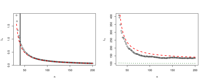
Figure 1: Drift parameters $\lambda$ and $L$ with data from a stable vector autoregression

NOTE: Circles correspond to observed $\lambda_{n}$ and $L_{n}$ calculated as in Lemma 5.1. Dashed lines are those $\lambda_{n}$ and $L_{n}$ but with $\hat{\mathcal{A}}$ and $Y^{\mathsf{T}}Q_{[Z,X]}Y/n$ replaced by $\mathcal{A}$ and $\Sigma$. The vertical line indicates $n=40$, the smallest $n$ for which $\lambda_{n}<1$. The dotted line is $L_{n}$ calculated as in Lemma 4.1; the $\lambda_{n}$ from that lemma is not shown because it can be taken to be $0$ for all $n$..

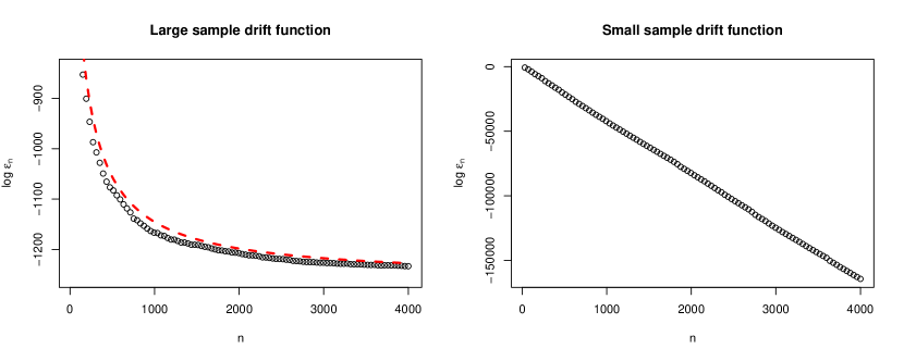
Figure 2: Minorization parameter $\varepsilon$ with data from a stable vector autoregression

NOTE: Circles correspond to observed $\log\varepsilon_{n}$, in the left plot calculated as in Lemma 5.2, with $T_{n}=2L_{n}(1-\lambda_{n})+10^{-6}$, and in the right plot as in Lemma 4.2 with $T_{n}=L_{n}+10^{-6}$. The dashed line is $\log\varepsilon_{n}$ with $\hat{\mathcal{A}}$ replaced by $\mathcal{A}$ and $Y^{\mathsf{T}}Q_{[Z,X]}Y/n$ replaced by $\Sigma$..

6 Discussion

Markov chain Monte Carlo is used in a wide range of problems, including but not limited to the Bayesian settings considered here. However, the theoretical properties of algorithms used by practitioners are not always well understood. We have focused on the case of Bayesian vector autoregressions with predictors. This is one of the most common models in time series, and in particular in the analysis and forecasting of macroeconomic time series. Moreover, due to similarities of the likelihoods of vector autoregressions and multivariate linear models, our results apply also to the latter. The Gibbs sampler has been suggested for exploring the posterior distribution of the parameters $\mathcal{A}$ and $\Sigma$ when there are no predictors [23], but there has been a lack of theoretical support. We have addressed this by proposing a collapsed Gibbs sampler that handles predictors and studying its convergence properties. Since our algorithm simplifies to the usual Gibbs sampler when there are no predictors, our results apply also in that setting.

We have proven that our algorithm generates a geometrically ergodic Markov chain under reasonable assumptions (Theorem 4.3). This result is applicable both in classical settings where the sample size is large (but fixed) in comparison to the number of parameters, and in large VARXs where the dimension of the process or the lag length is large in comparison to the number of observations. Though we have not emphasized it, this geometric ergodicity holds also if the model is misspecified. Indeed, once the data are fixed and the posterior specified, it is of no importance for the convergence rate how the data were actually generated, as long as they satisfy the conditions laid out in the relevant lemmas and theorem. Thus, with the algorithm we consider, characteristics of the posterior distribution can be reasonably estimated using principled approaches to ensuring the simulation results are trustworthy [7, 20, 48]. Our asymptotic analysis, or convergence complexity analysis, indicates our algorithm should perform well also in large samples; we have proven that, as the sample size tends to infinity, the geometric ergodicity of the sequence of transition kernels corresponding to our algorithm is asymptotically stable. This result is one of the first of its kind for practically relevant MCMC algorithms. As with our results for small samples, our asymptotic results hold under almost arbitrary model mispecification, as specified in Theorem 5.3.

Avenues for future research include convergence complexity analysis of cases where the dimension of the process or the lag length tends to infinity, either together with the sample size or for a fixed sample size. Our proof uses the intuition that the posterior concentrates near the least squares estimator, and it may be possible to formalize this intuition also in settings where $r$, $p$, or $q$ grows with $n$. However, it is likely that the drift function would need to be adjusted, perhaps by using a different norm: the Frobenius norm has convenient properties that we used in our proofs but is often less useful in high-dimensional settings [45]. If the sample size is fixed or grows slowly in comparison to other quantities, one would likely have to use a different drift function altogether or move to an approach that avoids the use of the minorization condition [33, 34].

Acknowledgements

The authors thank an Associate Editor, two reviewers, and Dootika Vats for suggestions and insightful comments that improved the paper. Ekvall gratefully acknowledges support by the FWF (Austrian Science Fund, https://www.fwf.ac.at/en/) [P30690-N35].

Appendix A Preliminaries

Lemma A.1.

If $X_{i}\in\mathbb{R}^{n\times m_{i}}$, $m_{i}\in\{1,2,\dots\}$, $i=1,2,3$, and $X=[X_{1},X_{2},X_{3}]$ $\in\mathbb{R}^{n\times(m_{1}+m_{2}+m_{3})}$ has full column rank, then with $\tilde{X}_{i}=Q_{X_{2}}X_{i}$, $i=1,2,3$,

1. $X_{1}^{\mathsf{T}}Q_{X_{2}}X_{1}$ is invertible,

2. $X_{1}^{\mathsf{T}}Q_{[X_{2},X_{3}]}X_{1}$ is invertible, and

3. $X_{1}^{\mathsf{T}}Q_{[X_{2},X_{3}]}X_{1}=\tilde{X}_{1}^{\mathsf{T}}Q_{\tilde{X}_{3}}\tilde{X}_{1}$.

Proof.

We start with 1. Suppose for contradiction that there exists $v\in\mathbb{R}^{m_{1}}\setminus\{0\}$ such that $X_{1}^{\mathsf{T}}Q_{X_{2}}X_{1}v=0$, which is equivalent to $Q_{X_{2}}X_{1}v=0$. This can happen either if $X_{1}v=0$, which contradicts the full column rank of $X$, or if $w=X_{1}v$ is a non-zero vector in the column space of $X_{1}$ that also lies in the column space of $X_{2}$, which again contradicts the full column rank of $X$. The proof for 2 is exactly the same as that of 1 but with $[X_{2},X_{3}]$ in place of $X_{2}$. Point 3 is an immediate consequence the Frisch–Waugh–Lovell theorem [29, Section 2.4], which says among other things that $Q_{\tilde{X}_{3}}\tilde{X_{1}}=Q_{[X_{2},X_{3}]}X_{1}$. ∎

Lemma A.2.

For any $A\in\mathbb{S}^{n}_{++}$, $B\in\mathbb{S}^{n}_{+}$, and invertible $C\in\mathbb{R}^{n\times n}$,

1. $\operatorname{tr}(C^{\mathsf{T}}[A+B]^{-1}C)\leq\operatorname{tr}(C^{\mathsf{T}}A^{-1}C)$,

2. $\|C^{\mathsf{T}}(A+B)^{-1}C\|\leq\|C^{\mathsf{T}}A^{-1}C\|$,

3. $|C^{\mathsf{T}}(A+B)C|\geq|C^{\mathsf{T}}AC|$, and

4. $|C^{\mathsf{T}}(A+B)^{-1}C|\leq|C^{\mathsf{T}}A^{-1}C|$.

Proof.

All claims can be reduced to the case where $C=I_{n}$ by either writing $C^{\mathsf{T}}(A+B)^{-1}C=(C^{-1}AC^{-\mathsf{T}}+C^{-1}BC^{-\mathsf{T}}])^{-1}$ and replacing $A$ and $B$ by $C^{-1}AC^{-\mathsf{T}}$ and $C^{-1}BC^{-\mathsf{T}}$, respectively, or by writing $C^{\mathsf{T}}(A+B)C=C^{\mathsf{T}}AC+C^{\mathsf{T}}BC$ and replacing $A$ and $B$ by $C^{\mathsf{T}}AC$ and $C^{\mathsf{T}}BC$, respectively. Assume thus that $C=I_{n}$. Since $A+B$ is SPD, the eigenvalues of $(A+B)^{-1}$ are the reciprocals of those of $A+B$. But, letting $\gamma_{i}(A)$ denote the $i$th eigenvalue in, say, decreasing order, Weyl’s inequalities [4, Corollary III.2.2] say $\gamma_{i}(A+B)\geq\gamma_{i}(A)+\gamma_{n}(B)=\gamma_{i}(A)+\gamma_{\min}(B)\geq\lambda_{i}(A)$, and hence $\operatorname{tr}([A+B]^{-1})=\sum_{i=1}^{n}1/\gamma_{i}(A+B)\leq\sum_{i=1}^{n}1/\gamma_{i}(A)=\operatorname{tr}(A^{-1})$, which proves the first claim. The remaining claims follow similarly since the spectral norm is the maximum eigenvalue for SPSD matrices and the determinant is the product of eigenvalues. ∎

Lemma A.3.

For any $X\in\mathbb{R}^{n\times p}$, $y\in\mathbb{R}^{n}$, and $c>0$,

$$\|(I_{p}c+X^{\mathsf{T}}X)^{-1}X^{\mathsf{T}}y\|\leq\|(X^{\mathsf{T}}X)^{g}X^{\mathsf{T}}y\|,$$

where superscript $g$ denotes an arbitrary generalized inverse.

Proof.

Consider the optimization problem of minimizing $g_{c}:\mathbb{R}^{p}\to[0,\infty)$ defined by

$$g_{c}(b):=\|y-Xb\|^{2}+c\|b\|^{2}.$$

If $c=0$, then any $b$ such that $X^{\mathsf{T}}Xb=X^{\mathsf{T}}y$ is a solution. Thus, for any generalized inverse, $b_{1}=(X^{\mathsf{T}}X)^{g}X^{\mathsf{T}}y$ solves the problem [12, Theorem 9.1.2]. On the other hand, if $c>0$ then since $Ic+X^{\mathsf{T}}X$ has full rank, the unique solution is $b_{2}=(cI+X^{\mathsf{T}}X)^{-1}X^{\mathsf{T}}y$. Now a contradiction arises if for some $c>0$, $\|b_{1}\|<\|b_{2}\|$, which finishes the proof. ∎

Lemma A.4.

For $A\in\mathbb{R}^{n\times n}$ and $B\in\mathbb{S}^{n}_{++}$, we have that $B^{-1}A^{g}B^{-1}$ is a generalized inverse of $BAB$, where superscript $g$ indicates a generalized inverse.

Proof.

We check the definition, namely that $BABB^{-1}A^{g}B^{-1}BAB=BAB$. Indeed, using that $AA^{g}A=A$, $BABB^{-1}A^{g}B^{-1}BAB=BAA^{g}AB=BAB$. ∎

Appendix B Main results

Proof Lemma 2.1.

Let us suppress conditioning on the parameters for simplicity. We have

$$f(Y,X) =f(X)f(Y\mid X)$$

$$=f(X)f(y_{1},\dots,y_{n}\mid X)$$

$$=f(X)f(y_{n}\mid y_{1},\dots,y_{n-1},X)f(y_{1},\dots,y_{n-1}\mid X)$$

$$=\ \vdots$$

$$=f(X)\prod_{t=1}^{n}f(y_{t}\mid y_{1},\dots,y_{t-1},X).$$

Consider an arbitrary term in the product. We have $Y_{t}=\mathcal{A}^{\mathsf{T}}Z_{t}+\mathcal{B}^{\mathsf{T}}X_{t}+U_{t}$. Since $Z_{t}$ is a function of $Y_{1},\dots,Y_{t-1}$, both $Z_{t}$ and $X_{t}$ are fixed when conditioning on $X$ and $Y_{1},\dots,Y_{t-1}$. Thus, the distribution of $Y_{t}\mid X,Y_{1},\dots,Y_{t-1}$ is determined by that of $U_{t}\mid X,Y_{1},\dots,Y_{t-1}$. But $Y_{1},\dots,Y_{t-1}$ are functions of $X_{1},\dots,X_{t-1}$ and $U_{1},\dots,U_{t-1}$, and $\{U_{t}\}$ is an i.i.d. sequence independent of $\{X_{t}\}$, and hence $X$. Thus, $U_{t}\mid X,Y_{1},\dots,Y_{t-1}\sim\mathcal{N}(0,\Sigma)$, and, consequently, $Y_{t}\mid X,Y_{1},\dots,Y_{t-1}\sim\mathcal{N}(\mathcal{A}^{\mathsf{T}}Z_{t}+\mathcal{B}^{\mathsf{T}}X_{t},\Sigma)$. Now the result follows by straightforward algebra and the fact that the distribution of $\{X_{t}\}$ does not depend on the model parameters. ∎

Proof Proposition 2.2.

Assuming the posterior is proper, the given expression for the density, up to scaling, follows from routine calculations. We prove the posterior is indeed proper under either of the two sets of conditions. Since

$$f(Y,X\mid\mathcal{A},\mathcal{B},\Sigma)=f(Y\mid\mathcal{A},\mathcal{B},\Sigma,X)f(X\mid\mathcal{A},\mathcal{B},\Sigma)=f(Y\mid\mathcal{A},\mathcal{B},\Sigma,X)f(X),$$

only the conditional density $f(Y\mid\mathcal{A},\mathcal{B},\Sigma,X)$ matters when deriving the posterior. Under either of the two sets of conditions, $X$ has full column rank so $X^{\mathsf{T}}X$ is invertible and we may define $H_{X}=(X^{\mathsf{T}}X)^{-1}X^{\mathsf{T}}$, $P_{X}=XH_{X}$, and $Q_{X}=I_{n}-P_{X}$. Let also $E=Y-Z\mathcal{A}$ and use $Q_{X}+P_{X}=I_{n}$ to write

$$f(Y\mid\mathcal{A},\mathcal{B},\Sigma,X)$$

$$\propto|\Sigma|^{-\frac{n}{2}}\operatorname{etr}\left(-\frac{1}{2}[X\mathcal{B}-E]^{\mathsf{T}}[X\mathcal{B}-E]\Sigma^{-1}\right)$$

$$=|\Sigma|^{-\frac{n}{2}}\operatorname{etr}\left(-\frac{1}{2}[X\mathcal{B}-E]^{\mathsf{T}}(Q_{X}+P_{X})[X\mathcal{B}-E]\Sigma^{-1}\right)$$

$$=|\Sigma|^{-\frac{n}{2}}\operatorname{etr}\left(-\frac{1}{2}E^{\mathsf{T}}Q_{X}E\Sigma^{-1}\right)\operatorname{etr}\left(-\frac{1}{2}[\mathcal{B}-H_{X}E]^{\mathsf{T}}X^{\mathsf{T}}X[\mathcal{B}-H_{X}E]\Sigma^{-1}\right).$$ (11)

The right-most term is a kernel of a matrix normal density for $\mathcal{B}$ with mean $H_{X}E$ and scale matrices $(X^{\mathsf{T}}X)^{-1}$ and $\Sigma$. Thus, integrating with respect to $\mathcal{B}$ gives,

$$\int f(Y\mid\mathcal{A},\mathcal{B},\Sigma,X)\,\mathrm{d}\mathcal{B} \propto|\Sigma|^{-\frac{n}{2}}\operatorname{etr}\left(-\frac{1}{2}E^{\mathsf{T}}Q_{X}E\Sigma^{-1}\right)(2\pi)^{rp/2}|X^{\mathsf{T}}X|^{-r}|\Sigma|^{p}$$

$$\propto|\Sigma|^{-\frac{n-p}{2}}\operatorname{etr}\left(-\frac{1}{2}E^{\mathsf{T}}Q_{X}E\Sigma^{-1}\right).$$

Thus, to show that $f(Y\mid\mathcal{A},\mathcal{B},\Sigma,X)f(\alpha)f(\Sigma)$ can be normalized to a proper posterior, we need only show that

$$\iint|\Sigma|^{-\frac{n-p}{2}}\operatorname{etr}\left(-\frac{1}{2}E^{\mathsf{T}}Q_{X}E\Sigma^{-1}\right)f(\alpha)f(\Sigma)\,\mathrm{d}\alpha\,\mathrm{d}\Sigma<\infty.$$ (12)

Let us consider the two sets of conditions separately, starting with the first. Since

$$\operatorname{tr}(E^{\mathsf{T}}Q_{X}E\Sigma^{-1})=\operatorname{tr}(\Sigma^{-1/2}E^{\mathsf{T}}Q_{X}E\Sigma^{-1/2})\geq 0,$$

we can upper bound the integrand in (12) by

$$|\Sigma|^{-\frac{n-p}{2}}f(\alpha)f(\Sigma)=|\Sigma|^{-\frac{n+a-p}{2}}\operatorname{etr}\left(-\frac{1}{2}\Sigma^{-1}D\right)f(\alpha),$$

which since we are assuming that $n-p+a-r-1>r-1$, i.e. that $n+a>2r+p$ and that $D$ is SPD, is the product of a proper inverse Wishart and a proper density for $\alpha$. This finishes the proof for the first set of conditions.

For the second set of conditions, notice that for (12) it suffices, since $D$ is SPSD, and hence $f(\Sigma)$ and $f(\alpha)$ both bounded, to show that

$$\iint|\Sigma|^{-\frac{n+a-p}{2}}\operatorname{etr}\left(-\frac{1}{2}E^{\mathsf{T}}Q_{X}E\Sigma^{-1}\right)\,\mathrm{d}\alpha\,\mathrm{d}\Sigma<\infty.$$

Let $\tilde{Y}=Q_{X}Y$ and $\tilde{Z}=Q_{X}Z$ so that $Q_{X}E=\tilde{Y}-\tilde{Z}\mathcal{A}$. Using the same decomposition as before we have for the last integrand

$$|\Sigma|^{-\frac{n+a-p}{2}}\operatorname{etr}\left(-\frac{1}{2}E^{\mathsf{T}}Q_{X}E\Sigma^{-1}\right)$$

$$=|\Sigma|^{-\frac{n+a-p-qr}{2}}\operatorname{etr}\left(-\frac{1}{2}\tilde{Y}^{\mathsf{T}}Q_{\tilde{Z}}\tilde{Y}\Sigma^{-1}\right)|\Sigma|^{-\frac{qr}{2}}$$

$$\quad\times\operatorname{etr}\left(-\frac{1}{2}[\mathcal{A}-H_{\tilde{Z}}\tilde{Y}]^{\mathsf{T}}\tilde{Z}^{\mathsf{T}}\tilde{Z}[\mathcal{A}-H_{\tilde{Z}}\tilde{Y}]\Sigma^{-1}\right).$$

Under the second set of assumptions, the last line is proportional to the product of an inverse Wishart density for $\Sigma$ with scale matrix $\tilde{Y}^{\mathsf{T}}Q_{\tilde{Z}}\tilde{Y}$ and $n+a-p-qr-r-1$ degrees of freedom and a matrix normal density for $\mathcal{A}$ with mean $H_{\tilde{Z}}\tilde{Y}$ and scale matrices $(\tilde{Z}^{\mathsf{T}}\tilde{Z})^{-1}$ and $\Sigma$, and hence integrable. The assumption that $[Y,X,Z]$ has full column ensures that, by Lemma A.1, $\tilde{Y}^{\mathsf{T}}Q_{\tilde{Z}}\tilde{Y}$ and $\tilde{Z}^{\mathsf{T}}\tilde{Z}$ are positive definite matrices. ∎

Proof of Lemma 3.1.

The full conditional distribution of $\mathcal{B}$ is immediate from dropping terms not depending on $\mathcal{B}$ in (B). Consider next the integrand in (12). The first term in the exponential is

$$\operatorname{tr}([Y-Z\mathcal{A}]^{\mathsf{T}}Q_{X}[Y-Z\mathcal{A}]\Sigma^{-1}) =\|Q_{X}(Y-Z\mathcal{A})\Sigma^{-1/2}\|_{F}^{2}$$

$$=\|(\Sigma^{-1/2}\otimes I_{n})(\operatorname{vec}(Q_{X}Y)-\operatorname{vec}(Q_{X}Z\mathcal{A}))\|^{2}$$

$$=\|(\Sigma^{-1/2}\otimes I_{n})(\operatorname{vec}(Q_{X}Y)-[I_{r}\otimes Q_{X}Z]\alpha)\|^{2}.$$

Thus, the log of the integrand is quadratic as a function of $\alpha$, with Hessian $-B=-\Sigma^{-1}\otimes Z^{\mathsf{T}}Q_{X}Z-C$ and gradient $-(\Sigma^{-1}\otimes Z^{\mathsf{T}}Q_{X})\operatorname{vec}(Q_{X}Y)-Cm$, which implies the desired distribution for $\alpha\mid\Sigma,Y$. Finally, the distribution of $\Sigma\mid\alpha,Y$ is immediate from dropping terms in the integrand in (12) not depending on $\Sigma$. ∎

Proof Lemma 3.2.

Assume $\alpha^{h},\mathcal{B}^{h},\Sigma^{h}$, $h=1,2,\dots$ are generated by the collapsed Gibbs sampler in Algorithm 1 started at some point $\theta^{0}\in\Theta$. The equality follows from showing that $\xi^{h}=(\alpha^{h},\Sigma^{h})$ and $\theta^{h}$ are co-de-initializing Markov chains [37, Corollary 1]. That they are both Markov chains is clear from the construction of the updates in Algorithm 1. That $\theta^{h}$ is de-initializing for $\xi^{h}$, i.e. that the distribution of $\xi^{h}\mid\theta^{h},\xi^{0}$ does not depend on $\xi^{0}$, is immediate from that $\xi^{h}$ is a function (coordinate projection) of $\theta^{h}$. The other direction, that $\xi^{h}$ is de-initializing for $\theta^{h}$, is by construction of the algorithm: since $\xi^{h}$ is a coordinate projection of $\theta^{h}$, the distribution of $\theta^{h}\mid\xi^{h},\theta^{0}$ is determined by that of $\mathcal{B}^{h}\mid\xi^{h},\theta^{0}$, and the distribution from which this value is drawn (line 4, Algorithm 1) does not depend on $\theta^{0}$. Similarly, notice that the distribution of $\xi^{h}\mid\xi^{h-1}$ is the same as $\xi^{h}\mid\alpha^{h-1}$ by construction of the algorithm. Thus, $\alpha^{h-1}$ is de-initializing for $\xi^{h}$ and the inequality follows [37, Theorem 1]. ∎

B.1 Inadequacy of Drift Function in Theorem 4.3

Proposition B.1.

For the $L=L_{n}(Y,X)$ defined in Lemma 4.1 it holds for some $c_{1}>0$ and $c_{2}>0$, depending on the hyperparameters but not the data, that

$$\|\hat{\alpha}\|_{F}^{2}\leq L_{n}(Y,X)\leq c_{1}\|\hat{\alpha}\|_{F}^{2}+c_{2},$$

and hence $L_{n}(Y,X)=O_{\mathsf{P}}(1)$ if and only if $\hat{\alpha}=O_{\mathsf{P}}(1)$.

Proof.

Since $C^{-1}$ is SPD, the term $\operatorname{tr}(C^{-1})$ is positive, and so dropping it and the term $\|C^{-1}\|\|Cm\|$ in the expression for $L_{n}(Y,X)$ gives

$$L_{n}(Y,X)>\|C^{-1/2}\|^{2}\|C^{1/2}\hat{\alpha}\|^{2}=\gamma_{\min}(C)^{-1}\|C^{1/2}\hat{\alpha}\|^{2}.$$

On the other hand, using that $(r_{1}+r_{2})^{2}\leq 2r_{1}^{2}+2r_{2}^{2}$ for any real numbers $r_{1}$ and $r_{2}$,

$$L_{n}(Y,X)\leq 2\|C^{-1}\|^{2}\|Cm\|^{2}+2\|C^{-1}\|\|C^{1/2}\hat{\alpha}\|^{2}+\operatorname{tr}(C^{-1}).$$

Now notice that $C-\gamma_{\min}(C)I_{qr^{2}}$ and $\gamma_{\max}(C)I_{qr^{2}}-C$ are both SPSD, and therefore

$$\gamma_{\min}(C)\|\hat{\alpha}\|^{2}\leq\hat{\alpha}^{\mathsf{T}}C\hat{\alpha}\leq\gamma_{\max}(C)\|\hat{\alpha}\|^{2}.$$

Thus, since $0<\gamma_{\min}(C)<\gamma_{\max}(C)<\infty$ and $\hat{\alpha}=\operatorname{vec}(\hat{\mathcal{A}})$, we are done. ∎

Proposition B.2.

If, almost surely as $n\to\infty$,

$$n\|Q_{X}Z\|^{2}/\|Q_{[Z,X]}Y\|^{2}\to\infty,$$

then the $\varepsilon=\varepsilon_{n}$ in Theorem 4.3 tends to zero almost surely as $n\to\infty$. In particular, $\varepsilon_{n}\to 0$ almost surely if $n^{-1}Y^{\mathsf{T}}Q_{[Z,X]}Y$ and $n^{-1}Z^{\mathsf{T}}Q_{X}Z$ have positive definite limits almost surely.

Proof.

Recall from Lemma 4.2 the definition of $\varepsilon=\varepsilon_{n}$, $c=n+a-p-r-1$, and $c_{1}=(\|Q_{X}Y\|+\|Q_{X}Z\|\sqrt{T})^{2}$. It suffices to show that $\zeta_{n}:=\varepsilon_{n}^{2n/c}\to 0$ almost surely since $2n/c\to 2$. We have

$$\zeta_{n}=\left[\frac{|D+Y^{\mathsf{T}}Q_{[Z,X]}Y|}{|D+I_{r}c_{1}|}\right]^{n}.$$

By Lemma A.2, $|D+Y^{\mathsf{T}}Q_{[Z,X]}Y|\leq|D+I_{r}\|Q_{[Z,X]}Y\|^{2}|$. Thus,

$$\zeta_{n}\leq\left[\frac{|D+I_{r}\|Q_{[Z,X]}Y\|^{2}|}{|D+I_{r}c_{1}|}\right]^{n}.$$

Now using that $c_{1}\geq\|Q_{X}Y\|^{2}+\|Q_{X}Z\|^{2}T$ and $\|Q_{X}Y\|\geq\|Q_{[Z,X]}Y\|$ in another application of Lemma A.2,

$$\zeta_{n}\leq\left[\frac{|D+I_{r}\|Q_{X}Y\|^{2}|}{|D+I_{r}\|Q_{X}Y\|^{2}+I_{r}\|Q_{X}Z\|^{2}T|}\right]^{n},$$

which can be written as a product of $r$ terms, the $j$th of which is

$$\left(1+\frac{d_{j}+T\|Q_{X}Z\|^{2}}{d_{j}+\|Q_{[Z,X]}Y\|^{2}}\right)^{-n},$$

where $d_{j}$ is the $j$th eigenvalue of $D$. Since $r$ is fixed, the product of $r$ terms tends to is zero if and only if one of the terms does, which happens unless $T\|Q_{X}Z\|^{2}/\|Q_{[Z,X]}Y\|^{2}=O(1/n)$ since $d_{j}$ is fixed. ∎

References

- [1] T. Abrahamsen and J. P. Hobert. Convergence analysis of block Gibbs samplers for Bayesian linear mixed models with . Bernoulli, 23:459–478, 2017.
- [2] G. Backlund and J. P. Hobert. A note on the convergence rate of MCMC for robust Bayesian multivariate linear regression with proper priors. Computational and Mathematical Methods, 2, 2020.
- [3] M. Bańbura, D. Giannone, and L. Reichlin. Large Bayesian vector autoregressions. Journal of Applied Econometrics, 25:71–92, 2009.
- [4] R. Bhatia. Matrix Analysis. Springer New York, 2012.
- [5] K. S. Chan and C. J. Geyer. Comment on “Markov chains for exploring posterior distributions”. The Annals of Statistics, 22:1747–1758, 1994.
- [6] C. R. Doss, J. M. Flegal, G. L. Jones, and R. C. Neath. Markov chain Monte Carlo estimation of quantiles. Electronic Journal of Statistics, 8:2448–2478, 2014.
- [7] J. M. Flegal, M. Haran, and G. L. Jones. Markov chain Monte Carlo: Can we trust the third significant figure? Statistical Science, 23:250–260, 2008.
- [8] J. M. Flegal and G. L. Jones. Batch means and spectral variance estimators in Markov chain Monte Carlo. The Annals of Statistics, 38:1034–1070, 2010.
- [9] J. M. Flegal and G. L. Jones. Implementing MCMC: Estimating with confidence. In S. Brooks, A. Gelman, X.-L. Meng, and G. L. Jones, editors, Handbook of Markov Chain Monte Carlo. Chapman & Hall, Boca Raton, 2011.
- [10] C. J. Geyer. Practical Markov chain Monte Carlo (with discussion). Statistical Science, 7:473–511, 1992.
- [11] S. Ghosh, K. Khare, and G. Michailidis. High-dimensional posterior consistency in Bayesian vector autoregressive models. Journal of the American Statistical Association, pages 1–14, 2018.
- [12] D. A. Harville. Matrix Algebra From a Statistician’s Perspective. Springer New York, 1997.
- [13] J. P. Hobert, Y. J. Jung, K. Khare, and Q. Qin. Convergence analysis of MCMC algorithms for Bayesian multivariate linear regression with non-Gaussian errors. Scandinavian Journal of Statistics, 2018.
- [14] R. A. Horn and C. R. Johnson. Topics in Matrix Analysis. Cambridge University Press, New York, 1991.
- [15] S. F. Jarner and E. Hansen. Geometric ergodicity of Metropolis algorithms. Stochastic Processes and Their Applications, 85:341–361, 2000.
- [16] J. E. Johndrow, A. Smith, N. Pillai, and D. B. Dunson. MCMC for imbalanced categorical data. Journal of the American Statistical Association, pages 1–10, 2018.
- [17] A. A. Johnson and G. L. Jones. Geometric ergodicity of random scan Gibbs samplers for hierarchical one-way random effects models. Journal of Multivariate Analysis, 140:325–342, 2015.
- [18] G. L. Jones. On the Markov chain central limit theorem. Probability Surveys, 1:299–320, 2004.
- [19] G. L. Jones, M. Haran, B. S. Caffo, and R. Neath. Fixed-width output analysis for Markov chain Monte Carlo. Journal of the American Statistical Association, 101:1537–1547, 2006.
- [20] G. L. Jones and J. P. Hobert. Honest exploration of intractable probability distributions via Markov chain Monte Carlo. Statistical Science, 16:312–334, 2001.
- [21] G. L. Jones and J. P. Hobert. Sufficient burn-in for Gibbs samplers for a hierarchical random effects model. The Annals of Statistics, 32:784–817, 2004.
- [22] K. R. Kadiyala and S. Karlsson. Numerical methods for estimation and inference in Bayesian VAR-models. Journal of Applied Econometrics, 12:99–132, 1997.
- [23] S. Karlsson. Forecasting with Bayesian vector autoregression. In Handbook of economic forecasting, pages 791–897. Elsevier, 2013.
- [24] G. M. Koop. Forecasting with medium and large Bayesian VARs. Journal of Applied Econometrics, 28:177–203, 2013.
- [25] D. Korobilis. Forecasting in vector autoregressions with many predictors. In Bayesian econometrics, pages 403–431. Emerald Group Publishing Limited, 2008.
- [26] K. Łatuszyński, B. Miasojedow, and W. Niemiro. Nonasymptotic bounds on the estimation error of MCMC algorithms. Bernoulli, 19:2033–2066, 2013.
- [27] J. S. Liu. The collapsed Gibbs sampler in Bayesian computations with applications to a gene regulation problem. Journal of the American Statistical Association, 89:958–966, 1994.
- [28] H. Lütkepohl. New Introduction to Multiple Time Series Analysis. Springer Berlin Heidelberg, 2005.
- [29] J. G. MacKinnon and R. Davidson. Econometric Theory and Methods. Oxford University Press, 2003-10-11, 2003.
- [30] J. R. Magnus and H. Neudecker. Matrix Differential Calculus With Applications in Statistics and Econometrics. Wiley John & Sons, 2002-07-11, 2002.
- [31] S. Meyn and R. L. Tweedie. Markov Chains and Stochastic Stability. Cambridge University Press, 2011.
- [32] Q. Qin and J. P. Hobert. Convergence complexity analysis of Albert and Chib’s algorithm for Bayesian probit regression. The Annals of Statistics, 47:2320–2347, 2019.
- [33] Q. Qin and J. P. Hobert. Geometric convergence bounds for Markov chains in Wasserstein distance based on generalized drift and contraction conditions. arXiv e-prints, page arXiv:1902.02964, 2019.
- [34] Q. Qin and J. P. Hobert. Wasserstein-based methods for convergence complexity analysis of MCMC with applications. arXiv e-prints, 2019.
- [35] B. Rajaratnam and D. Sparks. MCMC-Based inference in the era of big data: A fundamental analysis of the convergence complexity of high-dimensional chains. arXiv e-prints, page arXiv:1508.00947, 2015.
- [36] C. P. Robert. Convergence control methods for Markov chain Monte Carlo algorithms. Statistical Science, 10(3):231–253, 1995.
- [37] G. O. Roberts and J. S. Rosenthal. Markov chains and de-initializing processes. Scandinavian Journal of Statistics, 28:489–504, 2001.
- [38] G. O. Roberts and R. L. Tweedie. Geometric convergence and central limit theorems for multidimensional Hastings and Metropolis algorithms. Biometrika, 83:95–110, 1996.
- [39] N. Robertson, J. M. Flegal, D. Vats, and G. L. Jones. Assessing and visualizing simultaneous simulation error. Journal of Computational and Graphical Statistics (to appear), 2020.
- [40] J. S. Rosenthal. Minorization conditions and convergence rates for Markov chain Monte Carlo. Journal of the American Statistical Association, 90:558–566, 1995.
- [41] J. S. Rosenthal. Analysis of the Gibbs sampler for a model related to James–Stein estimators. Statistics and Computing, 6:269–275, 1996.
- [42] J. R. Schott. Matrix Analysis for Statistics. Wiley, Hoboken, New Jeresy, second edition, 2005.
- [43] R. L. Smith. Some interlacing properties of the Schur complement of a Hermitian matrix. Linear Algebra and its Applications, 177:137–144, 1992.
- [44] G. C. Tiao and A. Zellner. On the Bayesian estimation of multivariate regression. Journal of the Royal Statistical Society. Series B (Methodological), 26:277–285, 1964.
- [45] J. A. Tropp. An introduction to matrix concentration inequalities. Foundations and Trends in Machine Learning, 8(1-2):1–230, 2015.
- [46] D. Vats. Geometric ergodicity of Gibbs samplers in Bayesian penalized regression models. Electronic Journal of Statistics, 11:4033–4064, 2017.
- [47] D. Vats, J. M. Flegal, and G. L. Jones. Strong consistency of multivariate spectral variance estimators in Markov chain Monte Carlo. Bernoulli, 24:1860–1909, 2018.
- [48] D. Vats, J. M. Flegal, and G. L. Jones. Multivariate output analysis for Markov chain Monte Carlo. Biometrika, 106:321–337, 2019.
- [49] J. Yang and J. S. Rosenthal. Complexity results for MCMC derived from quantitative bounds. arXiv e-prints, 2019.
- [50] Y. Yang, M. J. Wainwright, and M. I. Jordan. On the computational complexity of high-dimensional Bayesian variable selection. The Annals of Statistics, 44:2497–2532, 2016.