Intrinsic Motivation Driven Intuitive Physics Learning using Deep Reinforcement Learning with Intrinsic Reward Normalization

Abstract

At an early age, human infants are able to learn and build a model of the world very quickly by constantly observing and interacting with objects around them. One of the most fundamental intuitions human infants acquire is intuitive physics. Human infants learn and develop these models, which later serve as prior knowledge for further learning. Inspired by such behaviors exhibited by human infants, we introduce a graphical physics network integrated with deep reinforcement learning. Specifically, we introduce an intrinsic reward normalization method that allows our agent to efficiently choose actions that can improve its intuitive physics model the most. Using a 3D physics engine, we show that our graphical physics network is able to infer object’s positions and velocities very effectively, and our deep reinforcement learning network encourages an agent to improve its model by making it continuously interact with objects only using intrinsic motivation. We experiment our model in both stationary and non-stationary state problems and show benefits of our approach in terms of the number of different actions the agent performs and the accuracy of agent’s intuition model.

1 Introduction

Various studies in human cognitive science have shown that humans rely extensively on prior knowledge when making decisions. Reinforcement learning agents require hundreds of hours of training to achieve human level performance in ATARI games, but human players only take couple hours to learn and play them at a competent level. This observation begs the question, what prior knowledge do humans have that accelerates their learning process? Recent works (Lake et al., 2017) suggest that there are two core ingredients which they call the ‘start-up software’: intuitive physics and intuitive psychology. These intuition models are present at a very early stage of human development and serve as core knowledge for future learning. But how do human infants build intuition models?

Figure 1: This diagram illustrates how an agent chooses an action based on loss incurred from its predictor which tries to mimic the behavior of an environment (or a subset of an environment). (1) After making an observation at time $t$, the agent’s actor module chooses an action. (2) The predictor module takes the action and the observation at time $t$ and makes a prediction; (3) the predictor module then compares its prediction to the observation from the environment at $t+1$ and (4) outputs a loss. (5) The loss value is converted into an intrinsic reward by the internal motivator module and is sent to the actor’s replay buffer to be stored for future training.

Imagine human infants in a room with toys lying around at a reachable distance. They are constantly grabbing, throwing and performing actions on objects; sometimes they observe the aftermath of their actions, but sometimes they lose interest and move on to a different object. The “child as scientist” view suggests that human infants are intrinsically motivated to conduct their own experiments, discover more information, and eventually learn to distinguish different objects and create richer internal representations of them (Lake et al., 2017). Furthermore, when human infants observe an outcome inconsistent with their expectation, they are often surprised which is apparent from their heightened attention (Baillargeon, 2007). The mismatch between expectation and actual outcome (also known as expectancy violations) have shown to encourage young children to conduct more experiments and seek more information (Stahl & Feigenson, 2015, 2017).

Inspired by such behaviors, in this paper, we explore intrinsically motivated intuition model learning that uses loss signals from an agent’s intuition model to encourage an agent to perform actions that will improve its intuition model (illustrated in Figure 1). Our contribution in this paper is twofold: (1) we propose a graphical physics network that can extract physical relations between objects and predict their physical behaviors in a 3D environment, and (2) we integrate the graphical physics network with the deep reinforcement learning network where we introduce the intrinsic reward normalization method that encourages the agent to efficiently explore actions and expedite the improvement of its intuition model. The results show that our actor network is able to perform a wide set of different actions and our prediction network is able to predict object’s change in velocity and position very accurately.

2 Approach

In this section, we explain representations of objects and their relations, followed by our internal motivator.

2.1 Representation

We represent a collection of objects as a graph where each node denotes an object and each edge represents a pairwise relation of objects. Due to its simple structure, we use sphere as our primary object throughout this paper. Given $N$ different objects, each object’s state, $s_{obj_{i}}$, consists of its features, $d_{obj_{i}}$, and its relations with other objects:

$$d_{obj_{i}} =[x,y,z,vx,vy,vz,r,m]\,,$$ (1)

$$r_{ij} =f_{r}(d_{obj_{i}},d_{obj_{j}})\,,$$ (2)

$$\mathbf{R}_{obj_{i}} =\begin{bmatrix}r_{i1}&r_{i2}&\cdots&r_{iN}\end{bmatrix}^{T}\,,$$ (3)

$$e_{obj_{i}} =\sum_{i\neq j,j\in[1,N]}r_{ij}\,,$$ (4)

$$s_{obj_{i}} =[d_{obj_{i}},e_{obj_{i}}]\,,$$ (5)

where $d_{obj_{i}}$ contains object’s Euclidean position $(x,y,z)$, Euclidean velocity $(vx,vy,vz)$, size $r$ and mass $m$. Some of these features are not readily available upon observation, and some works have addressed this issue by using convolutional neural networks (Lerer et al., 2016; Watters et al., 2017; Fragkiadaki et al., 2015); in this paper, we assume that these features are known for simplicity. To provide location invariance, we use an object-centric coordinate system, where the xy origin is the center of the sphere’s initial position and the z origin is the object’s initial distance to a surface (e.g. floor).

Relation Encoder

An object’s state also includes its pairwise relations to other objects. A relation from object $i$ to object $j$ is denoted as $r_{ij}$ and can be computed from the relation encoder, $f_{r}$, that takes two different object features, $d_{obj_{i}}$ and $d_{obj_{j}}$, and extracts their relation $r_{ij}$ (shown in Eq. (2)). Note that $r_{ij}$ is directional, and $r_{ij}\neq-r_{ji}$. Once all of object’s pairwise relations are extracted, they are stored in a matrix, $\mathbf{R}_{obj_{i}}$. The sum of all pairwise relations of an object yields $e_{obj_{i}}$, and when concatenated with the object feature $d_{obj_{i}}$, we get the state of the object $s_{obj_{i}}$.

An observation is a collection of every object’s state and its pairwise relations:

$$obs=[(s_{obj_{1}},\mathbf{R}_{obj_{1}}),(s_{obj_{2}},\mathbf{R}_{obj_{2}})),\cdots,(s_{obj_{n}},\mathbf{R}_{obj_{n}})]\,.$$

2.2 Object-based Attention

When an agent performs an action on an object, two things happen: (1) the object on which action was performed moves and (2) some other object (or objects) reacts to the moving object. Using the terms defined by (Chang et al., 2016), we call the first object focus object and the other object relation object. Given the focus object and the relation object, we associate agent’s action to the observation of both focus object and relation object. The agent’s job is to monitor the physical behaviors of both objects when selected action is performed and check whether its action elicited intended consequences.

2.3 Internal Motivator

ATARI games and other reinforcement learning tasks often have clear extrinsic rewards from the environment, and the objective of reinforcement learning is to maximize the extrinsic reward. In contrast, intuition model learning does not have any tangible reward from the external environment. For example, human infants are not extrinsically rewarded by the environment for predicting how objects move in the physical world.

In order to motivate our agent to continuously improve its model, we introduce an internal motivator module. Similar to the work of (Pathak et al., 2017), the loss value from an intuition model of an agent is converted into a reward by the internal motivator module $\phi$:

$$r_{t}^{intrinsic}=\phi(loss_{t})\,,$$ (6)

where $r_{t}^{intrinsic}$ is the intrinsic reward at time $t$, and $loss_{t}$ is loss from a prediction network at time $t$.While not having any extrinsic reward may result in ad hoc intrinsic reward conversion methods, we show that our model actually benefits from our simple, yet effective intrinsic reward normalization method. Note that while our method adopted to use the prediction error as the loss based on a prior work (Pathak et al., 2017; Burda et al., 2019), our approach mainly focuses on constructing an intuitive physics model, while the prior approaches are designed for the curiosity-driven exploration in a game environment.

Intrinsic Reward Normalization In conventional reinforcement learning problems, the goal of an agent is to maximize the total reward. To do so, it greedily picks an action with the greatest Q value. If that action does indeed maximize the overall reward, the Q value of that action will continue to increase until convergence. However, sometimes this could cause an agent to be stuck in a sub-optimal policy in which the agent is oblivious to other actions that could yield a greater total reward.

To ameliorate the problem of having a sub-optimal policy, the most commonly used method is a simple $\epsilon$-greedy method, which randomly chooses an action with $\epsilon$ probability. This is a simple solution, but resorts to randomly picking an action for exploration. An efficient way for exploration in stationary state setting with discrete actions is to use the upper confidence bound (UCB) action selection (Sutton & Barto, 1998):

$$a_{t}=\operatorname*{arg\,max}_{a}\Big{[}Q_{t}(a)+c\sqrt{\frac{\ln{t}}{N_{t}(a)}}\Big{]}\,,$$

where $Q_{t}(a)$ is the Q value of action $a$ at time $t$, $N_{t}(a)$ is the number of times action $a$ was chosen. However, this method has several shortcomings: (1) it is difficult to be used in non-stationary states since UCB does not take states into account, and (2) it can be more complex than $\epsilon$-greedy method since it needs to keep track of the number of actions taken. Notice that this heuristic assumes that Q value of some action $a$ at time $t$, or $Q_{t}(a)$, converges to some upper bound $\mathcal{U}\in\mathbb{R}$; i.e., $Q_{t}(a)\to\mathcal{U}^{-}$ as $t\to\infty$.

Intuitive physics learning is, however, slightly different from that of conventional reinforcement learning in that $\lim\limits_{t\to\infty}Q_{t}(a)=0$ $\ \forall a$. To show this, assuming that our intuition model improves in accuracy, it is equivalent to saying that loss is decreasing: $loss_{t}\to 0\text{ as }t\to\infty\,.$ Earlier, we defined our intrinsic reward $r^{intrinsic}_{t}=\phi(loss_{t})$ at Eq. (6). Since $loss_{t}\to 0$, we know that $r_{t}^{intrinsic}\to 0$ as long as $\phi$ is a continuous and increasing function. In both stationary and non-stationary state problems, if we train $Q_{t}(a)$ to be $r_{t}^{intrinsic}$, we can show that $\lim\limits_{t\to\infty}Q_{t}(a)=0$.

In order to capitalize on this property, we first normalize $\phi(loss_{t})$ by some upper bound $\mathcal{U}$ to get a normalized reward:

$$R^{intrinsic}_{t}=\frac{\phi(loss)}{\mathcal{U}}\,,$$ (7)

which restricts $R^{intrinsic}_{t}\in[0,1]$. Additionally, we normalize all $Q_{t}(a)$ by using the following equation, which is also known as the Boltzmann distribution of actions (Sutton & Barto, 1998):

$$\mathcal{Q}_{t}(a) =\Big{[}\frac{e^{Q_{t}(a)}}{\sum_{k=1}^{|A|}e^{Q_{t}(k)}}\Big{]}\,,$$ (8)

$$A_{t} =\operatorname*{arg\,max}_{a^{\prime}}\mathcal{Q}_{t}(a^{\prime})\,,$$ (9)

where $\mathcal{Q}_{t}(a)$ is the normalized Q value of action $a$ at time $t$, $|A|$ is the cardinality of the discrete action space, and $A_{t}$ is the action with the highest, normalized Q value.

Given $\mathcal{Q}_{t}(a)\in[0,1]$ and $R^{intrinsic}_{t}\in[0,1]$, as we train $\mathcal{Q}_{t}(a)$ with $R^{intrinsic}_{t}$ using gradient descent, this will naturally increase $Q_{t}(a)$ of actions that have not been taken according to our normalization step (Eq. (8)); i.e., $Q_{t}(a^{\prime})$ of $a^{\prime}$ actions that have been taken decreases and thus other actions that were not taken will have relatively bigger Q values.

Figure 2: This shows a detailed diagram of our overall approach shown in Fig. 1. (Bottom Right) For every pair of objects, we feed their features into our relation encoder to get relation $r_{ij}$ and object i’s state $s_{obj_{i}}$. (Top Left) Using the greedy method, for each object, we find the maximum Q value to get our focus object, relation object, and action. (Top Right) Once we have our focus object and relation object, we feed their states and all of their relations into our decoders to predict the change in position and change in velocity.

Compared to other methods such as UCB, our method has the benefit of not needing to explicitly keep track of the number of actions taken, and instead takes advantage of the decreasing behavior of loss values to encourage exploration. Moreover, because our method does not keep track of actions, it can be used in non-stationary state problems as well, which we show later in Sec. 5.

2.4 Replay Buffers

Our agent has two separate replay buffers: one to store object’s reward values to train the actor (actor replay buffer) and another to store the physical behaviors of objects to train the intuitive physics model (prediction replay buffer). For both networks, past experiences are sampled uniformly despite the fact that human brains are able to selectively retrieve past experiences from memory.

Despite uniform sampling, as our agent continuously experiments with objects, both replay buffers are more likely to contain experiences that the agent predicted with low accuracy. This is because our agent will greedily choose an action with the greatest Q value as shown in Eq. (9) and by design, action with the greatest Q value also has the greatest loss (equivalently low accuracy) by Eq. (7). Nonetheless, if the replay buffer is not big enough, this could let the agent overfit its intuitive physics model to experiences with high stochasticity. An ideal solution is to let agent curate its replay buffer content to find a set of experiences that can maximize the generalizability of the network. There are works that have addressed similar issues such as prioritized replay buffer (Schaul et al., 2015). However, we use uniform sampling in our work for its simplicity.

3 Network Models

Using deep neural networks, our agent network can be separated into three different sub-networks: relation encoders, deep Q network, and position & velocity decoders, illustrated in Fig. 2.

3.1 Deep Q Network

Inspired by the recent advances in deep reinforcement learning  (Mnih et al., 2015; Schulman et al., 2015, 2017; Silver et al., 2014), we use the object oriented  (Diuk et al., 2008) deep Q network to choose three things: (1) focus object, (2) relation object, and (3) action.

For each object, our deep Q network takes $\mathbf{R}_{obj_{i}}$ and $s_{obj_{i}}$ as input and computes $(N-1)\times|A|$ matrix, whose column represents action Q values and row represents $obj_{i}$’s relation object. Computing this for all objects, the final output of the network has a shape of $N\times(N-1)\times|A|$, which we call $\mathcal{Q}$, shown in the top left module

in Fig. 2. Our agent greedily finds focus object, relation object and action:

$$\textit{focus object, relation object, action}=\operatorname*{arg\,max}_{i,r,a}\mathcal{Q}_{i,r,a}\,,$$

where $i$ indicates the focus object index, $r$ is the relation object index, and $a$ denotes the action index.

Our deep Q network does not use a target network, and the actor replay buffer samples experiences of every object, instead of randomly sampling from all experiences uniformly. This is done to prevent an agent from interacting with only one object and from generalizing the behavior of one object to other objects.

With this setup, we set our stationary state target Q value, $y^{s}_{t}$, to be:

$$y^{s}_{t}=R^{t}_{intrinsic}\,,$$

and non-stationary state target Q value, $y^{ns}_{t}$, to be

$$y^{ns}_{t}=\begin{cases}R^{intrinsic}_{t}\hskip 19.91684pt\text{if reset occurs at t+1 }\\ \min(1,(R^{intrinsic}_{t}+\gamma\max_{a^{\prime}}Q_{a^{\prime}}(s_{obj_{i}}^{t+1})))\text{ o.w.}&\end{cases},$$ (10)

where $\gamma$ is a discount factor in $[0,1]$ and objects’ states reset when one of the objects goes out of bounds. We provide details of non-stationary state experiment and bounds in Sec. 4. For stationary state problems, since there is only single state, we only use $R^{intrinsic}_{t}$ to update our Q value. For non-stationary problems, we take the subsequent state into account and update the Q value with the sum of reward and discounted next state Q value. Note that our Q values and rewards reside in $[0,1]$ because of the reward normalization method; therefore, when the sum of reward and discounted next state reward exceeds 1, we clip the target value to 1.

3.2 Position & Velocity Decoders

The predicted position and velocity of each object is estimated by the predictor module which is placed inside a green box in Fig. 2).

An object’s state, $s_{obj_{i}}$ and all of its pairwise relations, $\mathbf{R}_{obj_{i}}$, are fed into both position and velocity decoders to predict the change in position and change in velocity of $obj_{i}$. For each pairwise relation, $r_{ij}$, we get an output $dpos_{i,r_{ij}}$ from the position decoder and $dvel_{i,r_{ij}}$ from the velocity decoder.

Once all relations are accounted for, the sum of all $dpos_{i,r_{ij}}$ and $dvel_{i,r_{ij}}$ are the final predicted change in position, $dpos_{obj_{i}}$, and predicted change in velocity, $dvel_{obj_{i}}$, of an object $i$:

$$dpos_{obj_{i}} =\sum_{i\neq j,j\in[1,N]}dpos_{obj_{i},r_{i,j}}\,,$$

$$dvel_{obj_{i}} =\sum_{i\neq j,j\in[1,N]}dvel_{obj_{i},r_{i,j}}\,,$$

We train both decoders and relation encoder with the sum of mean squared errors of positions and velocities:

$$loss=\sum_{k=\{i,r\}} ||dpos_{obj_{k}}-dpos^{\prime}_{obj_{k}}||_{2}$$

$$+||dvel_{obj_{k}}-dvel^{\prime}_{obj_{k}}||_{2}\,,$$

where $i$ is the focus object index and $r$ is the relation object index. $dpos^{\prime}_{obj_{k}}$ and $dvel^{\prime}_{obj_{k}}$ are the ground truth change in position and velocity of an object, and are readily available by the physics engine.

4 Experiment Setup

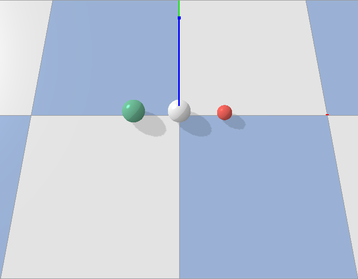
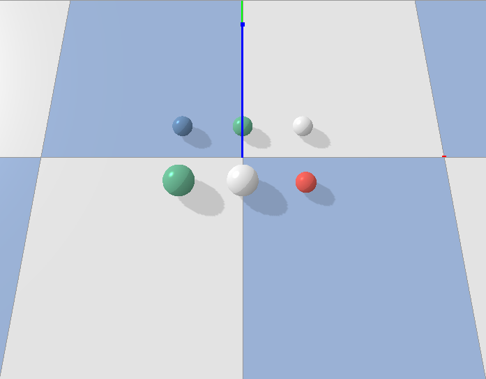
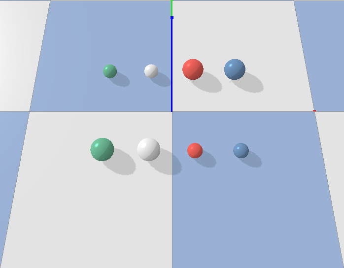
Objects In our experiment, we use spheres as primary objects due to its simple structure (i.e. we can represent an object with only one variable - radius). We use the center of the sphere as its xy position and its distance to a surface, i.e. floor, as z position. We used pybullet as our physics simulator with timestep of 1/240 seconds with 30 fps. As shown in Figure 3, we use three different scenes: 3-object, 6-object, and 8-object scenes. Objects are color coded so that each denotes different weight: red is 1kg, green is 0.75kg, blue is 0.5kg, and white is 0.25kg. Each object can have radius of 5cm or 7.5cm.

Figure 3: Experiments in three different scenes: 3-object, 6-object and 8-object scenes. Colors represent different weights where red is 1kg, green is 0.75kg, blue is 0.5kg and white is 0.25kg. The radius of each object can be either 5cm or 7.5cm. We experiment in two scenarios: stationary and non-stationary states.

Normalized Action Space We provide an agent with actions in three different directions: x, y and z. We experiment with a set of 27 actions ($x,y\in\{-1.0,0.0,1.0\}$ and $z\in\{0.0,0.75,1.0\}$), and a set of 75 actions ($x,y\in\{-1.0,-0.5,0.0,0.5,1.0\}$ and $z\in\{0.0,0.75,1.0\}$). An action chosen from the Q network is then multiplied by the max force, which we set to 400N.

Performance Metric Unlike conventional reinforcement learning problems, our problem does not contain any explicit reward that we can maximize on. For that reason, there is no clear way to measure the performance of our work. Outputs from both prediction network and deep Q network rely heavily on how many different actions the agent has performed. For instance, if an agent performs only one action, the prediction loss will converge to 0 very quickly, yet agent would have only learned to predict the outcome of one action. Therefore, we provide the following performance metrics to see how broadly our agent explores different actions and how accurately it predicts outcomes of its actions:

Table 1: Stationary state Action Coverage We record the number of interactions our agent takes to perform actions in three different scenes. Each scene was experimented with two or more trials with different random seeds. We stop training when interaction count exceeds 75000 interactions.

	#Actions per relation	Total # Actions	Action Coverage	Interaction Count
3-Object Scene	27	162	1.0	$770.38\pm 187.914$
	75	450	1.0	$2505.6\pm 401.968$
6-Object Scene	27	810	1.0	$7311.0\pm 2181.74$
	75	2250	1.0	$25958.67\pm 3609.25$
8-Object Scene	27	1512	1.0	$22836\pm 2225.0$
	75	4200	$0.8\pm 0.107$	$75000$

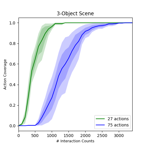
• Action Coverage We measure the percentage of actions covered by an agent. There are in total of $N\times(N-1)\times|A|$ many actions for all pairs of objects. We use a binary matrix, $M$, to keep track of actions taken. We say that we covered a single action when an agent performs that action on all object relation pairs for every focus object. In short, if $\prod_{i,r}M_{i,r,a_{k}}=1\text{ for some action $a_{k}$}$, then we say it covered the action $a_{k}$. Action coverage is then computed by $(\sum_{a}\prod_{i,r}M_{i,r,a})/|A|$. Action coverage value will tell us two things: (1) whether our predictor module is improving and (2) whether our agent is exploring efficiently. If the predictor module is not improving, the intrinsic reward associated with that action will not decrease, causing the agent to perform the same action repeatedly.

• Prediction Error Once an agent has tried all actions, we use prediction error to test whether agent’s predictor module improved.

For other hyperparameters, we set the upper bound $\mathcal{U}$ to be infinity and $\phi$ to be an identity function.

5 Experiments

In this section, we provide results of our experiments in stationary and non-stationary state problems.

5.1 Stationary State (Multi-armed Bandit Problem)

In stationary state, or multi-arm bandit problem, after an agent takes an action, we reset every object’s position back to its original state. The initial states of objects in different scenes are shown in Figure 3. We test with two different action sets and compare the number of interactions it takes for an agent to try out all actions. We also test generalizability of our agent’s prediction model to multiple objects.

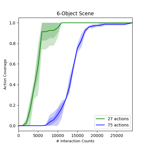
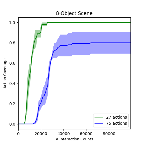
Action Coverage As shown in Table 1, our agent successfully tries all available actions in 3-object and 6-object scenes for both set of actions. Despite the huge number of actions, our agent is able to intrinsically motivate itself to perform hundreds and thousands of actions. While there is no clear way to tell our method is the fastest, we are not aware of any previous work that measures the number of actions covered by an agent, since conventional reinforcement learning problems do not require an agent to perform all actions. The fastest way to cover all actions is to keep track of all actions and their Q values in a table; however, this method has scalability issues and cannot be extended to non-stationary state problems.

As number of actions increases, it, however, takes longer for our agent to cover all actions. In fact, for 8-object scene, it fails to achieve full action coverage when presented with 75 different actions per object. One possible explanation of this is the replay buffer. Using a sampling batch size of 1024, the actor replay buffer uniformly samples 1024 past experiences for all objects. For 8-object scene with 75 actions, each object has 525 unique actions per all pairs of objects. Compared to other scenes, the probability of getting 525 unique action experiences from 1024 samples is a lot lower, especially when the actor replay buffer has uneven distribution of actions.

To make matters worse, our prediction replay buffer is limited in size. In our experiment, the prediction buffer of size $2.5e+6$ saturates before our agent can perform all actions.. It is apparent that our approach cannot scale to scenes with more objects and actions with the current implementation of both actor and prediction replay buffers. We leave the improvement of replay buffers to future work.

Figure 4: Action coverage results after 3 or more runs with different random seeds. (From left to right) Action coverage of our agent in 3-object, 6-object, and 8-object scene.

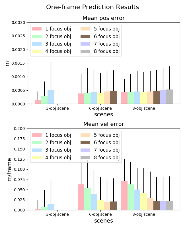
Prediction Error To test whether our agent’s intuitive physics model predicts object position and velocity correctly, we test it by computing the $L2$-norm between predicted and the actual position and velocity of object after one frame. Our agent’s prediction model errors are plotted in Figure 5. For all scenes, the position errors of one frame prediction are within 0.002m and the velocity errors are within 0.15m/s. These errors quite small, given the fact that the objects in our scene can change its position from 0 to 0.18465m per frame and velocity change ranges from 0 to 6.87219m/s per frame.

Our prediction error could be reduced further with other network architectures. In fact, there are many works that are trying to develop better network models for intuitive physics learning. However, the aim of our work is to show that the loss value from any intuitive physics network can be converted into an intrinsic reward to motivate an agent to explore different actions. Observations from different actions result in a diverse set of training data, which can make the intuitive physics network more general and robust.

In generalization tasks, we allow our agent to apply forces on multiple objects and see if it can predict the outcome after one frame. We generate 100 experiments by randomly selecting focus objects and actions. We let our agent to predict the next position and velocity of all objects in the scene, and we measure the mean error of all predictions. Video of our results can be found in supplementary video 1. The results show that our agent’s prediction network accurately predicts the physical behavior of colliding and non-colliding objects. Moreover, our agent’s intuition model is able to generalize to multiple moving objects very well even though the agent was only trained with an observation of a pair of objects (i.e.focus and relation object). Our qualitative results show that the agent’s prediction model is able to predict that collision causes a moving object to either deflect or stop, and causes idle objects to move. Additionally, despite not knowing about gravitational forces, it learns that objects fall when they are above a surface.

While there are other intuitive physics networks trained with supervised learning that can yield a higher accuracy, it is difficult for us to compare our results with theirs. The biggest reason is that supervised learning requires a well-defined set of training data a priori. In our work and reinforcement learning in general, data are collected by an agent, and those data are not identical to that of supervised learning, making it difficult to compare two different approaches in a fair setting. Additionally, the training process differs: supervised learning takes epoch based learning where it iterates over the same dataset multiple times until the network reaches a certain error rate on a validation set. In deep reinforcement learning, a small subset of data is randomly sampled from the replay buffer and is used to train the network on the fly.

5.2 Non-stationary State (Reinforcement Learning)

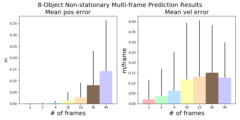
We extend our prediction model with deep Q network to non-stationary state problems where we do not reset the objects unless they go out of bounds. To increase the chance of collision, we provide 9 actions only on the $xy$ place (i.e. $x,y\in\{-1,0,1\}$). We arbitrarily set the bounds to be $3m\times 3m$ square. Since there are no walls to stop objects from going out of bounds, objects have a low probability of colliding with another object. In order to make them collide on every interaction, we generated 51 test cases in which every interaction causes a collision among objects. Our agent’s prediction model then predicts the object’s location after varying number of frames (i.e. 1,2,4,10,15,30,45 frames).

Prediction Error Prediction network’s errors are plotted in Figure 6. We see that when our agent predicts object locations after 1, 2, and 4 frames, the error is negligibly small. However, our agent is uncertain when predicting object location after 10 or more frames. This is because the error from each frame accumulates and causes objects to veer away from the actual path. Our qualitative results of non-stationary problem can be found in supplementary video 2. Similar to stationary state results, our agent’s prediction network accurately predicts an object’s general direction and their movements, despite having infinitely many states. The agent’s prediction network is able to predict whether an object will stop or deflect from its original trajectory when colliding with another object. Even if the agent’s prediction network fails to predict the correct position of a moving object, it still makes a physically plausible prediction.

Limitation We would like to point out that although our agent performed thousands of interactions, our agent still fails to learn that objects do not go through one another, as seen in our qualitative results. This is very noticeable when objects are moving fast. We conjecture that once our agent makes a wrong prediction, the predicted object overlaps with another object, causing our agent fails to predict subsequent positions and velocities. One plausible explanation is that it has never seen such objects overlap in its training data, hence fails to predict it accurately.

Figure 5: Mean position and velocity prediction errors after 1 frame with different number of focus objects in 3-object, 6-object, and 8-object scene.

6 Background

Figure 6: We test our intuition model in the non-stationary problem. Fewer prediction steps incur almost no error, while higher prediction steps, i.e. more than 4 frames, incur a high loss due to cumulative errors.

6.1 Deep Reinforcement Learning

Recent advances in deep reinforcement learning have achieved super-human performances on various ATARI games (Mnih et al., 2015) and robotic control problems (Schulman et al., 2015, 2017; Silver et al., 2014). While these approaches have achieved state-of-the-art performances on many tasks, they are often not easily transferable to other tasks because these networks are trained on individual tasks.

As opposed to model-free methods, model-based approaches create a model of an environment, which equips agents with the ability to predict and plan. Dyna-Q, proposed by (Sutton, 1990), integrated model-free with model-based learning so an agent can construct a model of an environment, react to the current state and plan actions by predicting future states. More recent work in model based reinforcement learning (Oh et al., 2017) proposed a value prediction network that learns a dynamic environment and predicts future values of abstract states conditioned on options.

6.2 Intrinsic Motivation and Curiosity

Early work by (Berlyne, 1966) showed that both animals and humans spend a substantial amount of time exploring that is driven by curiosity. Furthermore, Berlyne’s theory suggests that curiosity, or intrinsic motivation (Barto et al., 2004; Chentanez et al., 2005), is triggered by novelty and complexity.

The idea of integrating curiosity, and its counterpart boredom, with reinforcement learning was suggested by (Schmidhuber, 1991), and showed that intrinsic reward can be modeled to motivate agents to explore areas with high prediction errors (Schmidhuber, 2010). Using deep learning, (Pathak et al., 2017) proposed an intrinsic curiosity module that outputs a prediction error in the state feature space, which is used as an intrinsic reward signal. Our work adopted this approach of using the prediction error for our intrinsic reward.

6.3 Intuitive Physics

At an early age, human infants are equipped with a “starter pack” (Lake et al., 2017), which includes a sense of intuitive physics. For instance, when observing a moving ball, our intuitive physics can sense how fast the ball is going and how far the ball will go before it comes to a complete halt. This intuitive physics is present as a prior model and accelerates future learning processes. Works done by (Battaglia et al., 2013) and (Hamrick, 2011) show that humans have an internal physics model that can predict and influence their decision making process.

Recent works have focused on using deep learning to model the human’s intuitive physics model. (Lerer et al., 2016) used a 3D game engine to simulate towers of wooden blocks and introduced a novel network, PhysNet, that can predict whether a block tower will collapse and its trajectories. (Fragkiadaki et al., 2015) proposed a visual predictive model of physics where an agent is able to predict ball trajectories in billiards. Another work by (Chang et al., 2016) proposed a neural physics engine that uses an object based representation to predict the state of the focus object given a physical scenario. (Battaglia et al., 2016) presented an interaction network that combined structured models, simulation, and deep learning to extract relations among objects and predict complex physical systems. We extend the previous works by integrating deep reinforcement learning that intrinsically motivates our agent to improve its physics model.

7 Discussion

In this paper, we have proposed a graphical physics network integrated with deep Q learning and a simple, yet effective reward normalization method that motivates agents to explore actions that can improve its model. We have demonstrated that our agent does indeed explore most of its actions, and our graphical physics network is able to efficiently predict object’s position and velocity. We have experimented our network on both stationary and non-stationary problems in various scenes with spherical objects with varying masses and radii. Our hope is that these pre-trained intuition models can later be used as a prior knowledge for other goal oriented tasks such as ATARI games or video prediction.

References

- Baillargeon (2007) Baillargeon, R. The Acquisition of Physical Knowledge in Infancy: A Summary in Eight Lessons, chapter 3, pp. 47–83. Wiley-Blackwell, 2007. ISBN 9780470996652. doi: 10.1002/9780470996652.ch3.
- Barto et al. (2004) Barto, A. G., Singh, S., and Chentanez, N. Intrinsically motivated learning of hierarchical collections of skills. In Proceedings of International Conference on Developmental Learning (ICDL). MIT Press, Cambridge, MA, 2004.
- Battaglia et al. (2016) Battaglia, P., Pascanu, R., Lai, M., Rezende, D. J., and kavukcuoglu, K. Interaction networks for learning about objects, relations and physics. In Proceedings of the 30th International Conference on Neural Information Processing Systems, NIPS’16, pp. 4509–4517, USA, 2016. Curran Associates Inc. ISBN 978-1-5108-3881-9.
- Battaglia et al. (2013) Battaglia, P. W., Hamrick, J. B., and Tenenbaum, J. B. Simulation as an engine of physical scene understanding. Proceedings of the National Academy of Sciences, 110(45):18327–18332, 2013. ISSN 0027-8424. doi: 10.1073/pnas.1306572110.
- Berlyne (1966) Berlyne, D. E. Curiosity and exploration. Science, 153(3731):25–33, 1966. ISSN 0036-8075. doi: 10.1126/science.153.3731.25.
- Burda et al. (2019) Burda, Y., Edwards, H., Pathak, D., Storkey, A., Darrell, T., and Efros, A. A. Large-scale study of curiosity-driven learning. In ICLR, 2019.
- Chang et al. (2016) Chang, M. B., Ullman, T., Torralba, A., and Tenenbaum, J. B. A compositional object-based approach to learning physical dynamics. arXiv preprint arXiv:1612.00341, 2016.
- Chentanez et al. (2005) Chentanez, N., Barto, A. G., and Singh, S. P. Intrinsically motivated reinforcement learning. In Saul, L. K., Weiss, Y., and Bottou, L. (eds.), Advances in Neural Information Processing Systems 17, pp. 1281–1288. MIT Press, 2005.
- Diuk et al. (2008) Diuk, C., Cohen, A., and Littman, M. L. An object-oriented representation for efficient reinforcement learning. In Proceedings of the 25th International Conference on Machine Learning, ICML ’08, pp. 240–247, New York, NY, USA, 2008. ACM. ISBN 978-1-60558-205-4. doi: 10.1145/1390156.1390187.
- Fragkiadaki et al. (2015) Fragkiadaki, K., Agrawal, P., Levine, S., and Malik, J. Learning visual predictive models of physics for playing billiards. CoRR, abs/1511.07404, 2015. URL http://arxiv.org/abs/1511.07404.
- Hamrick (2011) Hamrick, J. Internal physics models guide probabilistic judgments about object dynamics. 01 2011.
- Lake et al. (2017) Lake, B. M., Ullman, T. D., Tenenbaum, J. B., and Gershman, S. J. Building machines that learn and think like people. Behavioral and Brain Sciences, 40:e253, 2017.
- Lerer et al. (2016) Lerer, A., Gross, S., and Fergus, R. Learning physical intuition of block towers by example. In Balcan, M. F. and Weinberger, K. Q. (eds.), Proceedings of The 33rd International Conference on Machine Learning, volume 48 of Proceedings of Machine Learning Research, pp. 430–438, New York, New York, USA, 20–22 Jun 2016. PMLR.
- Mnih et al. (2015) Mnih, V., Kavukcuoglu, K., Silver, D., Rusu, A. A., Veness, J., Bellemare, M. G., Graves, A., Riedmiller, M., Fidjeland, A. K., Ostrovski, G., Petersen, S., Beattie, C., Sadik, A., Antonoglou, I., King, H., Kumaran, D., Wierstra, D., Legg, S., and Hassabis, D. Human-level control through deep reinforcement learning. Nature, 518(7540):529–533, 02 2015.
- Oh et al. (2017) Oh, J., Singh, S., and Lee, H. Value prediction network. In Guyon, I., Luxburg, U. V., Bengio, S., Wallach, H., Fergus, R., Vishwanathan, S., and Garnett, R. (eds.), Advances in Neural Information Processing Systems 30. 2017.
- Pathak et al. (2017) Pathak, D., Agrawal, P., Efros, A. A., and Darrell, T. Curiosity-driven exploration by self-supervised prediction. In ICML, 2017.
- Schaul et al. (2015) Schaul, T., Quan, J., Antonoglou, I., and Silver, D. Prioritized experience replay. CoRR, abs/1511.05952, 2015.
- Schmidhuber (1991) Schmidhuber, J. A possibility for implementing curiosity and boredom in model-building neural controllers, 1991.
- Schmidhuber (2010) Schmidhuber, J. Formal theory of creativity, fun, and intrinsic motivation (1990–2010). IEEE Transactions on Autonomous Mental Development, 2(3):230–247, Sept 2010. ISSN 1943-0604. doi: 10.1109/TAMD.2010.2056368.
- Schulman et al. (2015) Schulman, J., Levine, S., Moritz, P., Jordan, M., and Abbeel, P. Trust region policy optimization. In Proceedings of the 32Nd International Conference on International Conference on Machine Learning - Volume 37, ICML’15, pp. 1889–1897. JMLR.org, 2015.
- Schulman et al. (2017) Schulman, J., Wolski, F., Dhariwal, P., Radford, A., and Klimov, O. Proximal policy optimization algorithms. CoRR, abs/1707.06347, 2017.
- Silver et al. (2014) Silver, D., Lever, G., Heess, N., Degris, T., Wierstra, D., and Riedmiller, M. Deterministic policy gradient algorithms. In Proceedings of the 31st International Conference on International Conference on Machine Learning - Volume 32, ICML’14, pp. I–387–I–395. JMLR.org, 2014.
- Stahl & Feigenson (2015) Stahl, A. E. and Feigenson, L. Observing the unexpected enhances infants’ learning and exploration. Science, 348(6230):91–94, 2015. ISSN 0036-8075. doi: 10.1126/science.aaa3799. URL http://science.sciencemag.org/content/348/6230/91.
- Stahl & Feigenson (2017) Stahl, A. E. and Feigenson, L. Expectancy violations promote learning in young children. Cognition, 163:1 – 14, 2017. ISSN 0010-0277. doi: https://doi.org/10.1016/j.cognition.2017.02.008. URL http://www.sciencedirect.com/science/article/pii/S0010027717300380.
- Sutton (1990) Sutton, R. S. Integrated architectures for learning, planning, and reacting based on approximating dynamic programming. In In Proceedings of the Seventh International Conference on Machine Learning, pp. 216–224. Morgan Kaufmann, 1990.
- Sutton & Barto (1998) Sutton, R. S. and Barto, A. G. Introduction to Reinforcement Learning. MIT Press, Cambridge, MA, USA, 1st edition, 1998. ISBN 0262193981.
- Watters et al. (2017) Watters, N., Zoran, D., Weber, T., Battaglia, P., Pascanu, R., and Tacchetti, A. Visual interaction networks: Learning a physics simulator from video. In Guyon, I., Luxburg, U. V., Bengio, S., Wallach, H., Fergus, R., Vishwanathan, S., and Garnett, R. (eds.), Advances in Neural Information Processing Systems 30, pp. 4539–4547. Curran Associates, Inc., 2017.