Path-integral dynamics of water using curvilinear centroids

Abstract

We develop a path-integral dynamics method for water that resembles centroid molecular dynamics (CMD), except that the centroids are averages of curvilinear, rather than cartesian, bead coordinates. The curvilinear coordinates are used explicitly only when computing the potential of mean force, the components of which are re-expressed in terms of cartesian ‘quasi-centroids’ (so-called because they are close to the cartesian centroids). Cartesian equations of motion are obtained by making small approximations to the quantum Boltzmann distribution. Simulations of the infrared spectra of various water models over 150–600 K show these approximations to be justified: for a two-dimensional OH-bond model, the quasi-centroid molecular dynamics (QCMD) spectra lie close to the exact quantum spectra, and almost on top of the Matsubara dynamics spectra; for gas-phase water, the QCMD spectra are close to the exact quantum spectra; for liquid water and ice (using the q-TIP4P/F surface), the QCMD spectra are close to the CMD spectra at 600 K, and line up with the results of thermostatted ring-polymer molecular dynamics and approximate quantum calculations at 300 and 150 K. The QCMD spectra show no sign of the CMD ‘curvature problem’ (of erroneous red shifts and broadening). In the liquid and ice simulations, the potential of mean force was evaluated on-the-fly by generalising an adiabatic CMD algorithm to curvilinear coordinates; the full limit of adiabatic separation needed to be taken, which made the QCMD calculations 8 times more expensive than partially adiabatic CMD at 300 K, and 32 times at 150 K (and the intensities may still not be converged at this temperature). The QCMD method is probably generalisable to many other systems, provided collective bead-coordinates can be identified that yield compact mean-field ring-polymer distributions.

I Introduction

A major challenge in molecular simulation is to include nuclear quantum effects in the dynamics of liquid water, ice, and related systems. One way to do this is to make local approximations around one water molecule, then to solve the Schrödinger equation in a reduced space.skinner2009 ; skinner2013 ; lmon1 ; lmon2 Another way, arguably more general, because it does not require a local approximation, is to use path-integrals to describe the quantum Boltzmann statistics exactly, and classical mechanics to approximate the dynamics. billjpc ; liubill ; liurev ; shig ; jens1 ; xantheas ; liuwat ; bonella ; vollume ; van1 ; van2 ; jerin1 ; jerin2 ; caov2 ; craig1 ; craig2 ; tfmiller1 ; annurev ; trpmd1 ; jorsca ; tim ; tom1 ; tom2 ; paes1 ; paes2 This type of approach assumes that real-time coherences mainly average out in condensed-phase systems, leaving most of the quantum effects in the statistics.

The oldest such ‘quantum statistics + classical dynamics’ approach is based on the classical Wigner, or LSC-IVR, approximation.billjpc ; liubill ; liurev ; shig ; jens1 This approach is powerful, and has been used to calculate infraredxantheas and recently Raman spectraliuwat for liquid water. However, LSC-IVR has the drawback that the classical trajectories do not conserve the quantum Boltzmann distribution, which has the effect of damping spectral lineshapes.

More recently, approaches such as centroid molecular dynamics (CMD)caov2 and (thermostatted) ring-polymer molecular dynamics ((T)RPMD)craig1 ; craig2 ; tfmiller1 ; annurev ; trpmd1 ; jorsca ; tim ; tom1 ; tom2 have been developed, which redress this problem by using trajectories that do conserve the quantum Boltzmann distribution. These approaches are very practical, since they can be run as extended classical MD simulations. But they also have drawbacks of their own.

The CMD method has proved to be useful for simulating water dynamics, most notably in recent calculations on the MB-pol ab initio water potential energy surface.paes1 ; paes2 The method works by generating classical trajectories on the free-energy surface obtained by mean-field averaging the quantum Boltzmann distribution around the centroids (centres-of-mass) of the ring-polymers (imaginary-time Feynman pathschanwol ; pariram ; ceperley ). However, CMD breaks down at low temperatures, when the mean-field ring-polymer distributions delocalise.trpmd2 ; marx09 ; marx10 When applied to gas-phase water, the CMD ring-polymer distribution spreads in a crescent around the curve of the rotating OH-bond, so that the centroid lies approximately at its focal point, which flattens the potential, and leads to an artificially red-shifted and broadened spectral lineshape. This ‘curvature problem’ is less severe in the condensed than the gas phase,marx10 since there is less spreading around librations than rotations, but it is still serious enough to give, e.g., a 100 cm^-1 red shift and considerable broadening to the OH-stretch band of ice at 150 K.trpmd2

The RPMD method does not suffer from the CMD curvature problem, since it involves no mean-field averaging, propagating instead all the ring-polymer ‘beads’ (imaginary-time replicas) as separate particles. However, the dynamics of the modes orthogonal to the centroid are fictitious, because of the ring-polymer spring-forces, and hence need to be damped by a thermostat to avoid corrupting the spectrum.trpmd1 ; trpmd2 ; trpmd3 This means that thermostatted (T)RPMD is an extremely efficient method for generating spectral line positions, but that it predicts lineshapes that are often too broad.

It would therefore be useful to develop a path-integral method which generates dynamics that is quantum Boltzmann conserving, but which manages to avoid both the curvature problem of CMD, and the fictitious springs of RPMD. In refs. marx09, ; marx10, , Marx and co-workers suggest that such a method could be developed by modifying CMD, such that the centroids are taken as the averages of curvilinear rather than cartesian bead coordinates. This curvilinear centroid would lie at the centre of the ring-polymer distribution, rather than at its approximate focal point, which would stop the free energy from artificially flattening. To our knowledge, this suggestion has not yet been pursued.

More recently, the case for curvilinear centroids has been strengthened further, by the development of ‘Matsubara dynamics’, which is the quantum-Boltzmann-conserving classical dynamics that results when the exact quantum dynamics is mean-field averaged to make it smooth and continuous in imaginary time.mats ; mf-mats Matsubara dynamics is impossible to compute exactly (except in toy systems), owing to a phase problem, but it can be computed approximately.jens2 ; planets ; mats-rpmd In fact CMD and TRPMD (both first obtained heuristically) are mean-field and short-time approximations to Matsubara dynamics.mats-rpmd By considering a two-dimensional model, it was shown that the CMD curvature problem in the OH stretch can be cured if just a few modes are released from the centroid-averaged mean-field.mf-mats The resulting Matsubara stretch bands are very close to the exact quantum results, the only significant error being a small, temperature-independent blue shift, which also affects CMD (when the temperature is high enough to avoid the curvature problem) and TRPMD. It was also found that the spreading of the CMD ring-polymer distribution around the rotational angle is exacerbated by artificial instantons, which form at small bond-lengths because of the cartesian centroid constraint.mf-mats Curvilinear centroids would avoid such artefacts, and should therefore give more compact distributions around the rotational angle, and thus a better approximation to the Matsubara-dynamics spectrum.

In this article, we investigate these likely advantages, by developing a method, called ‘quasi-centroid molecular dynamics’ (QCMD), which applies curvilinear centroid dynamics to water. We have not tried formally to derive QCMD from Matsubara dynamics—such a derivation is almost certainly possible, but we thought it best first to test QCMD numerically.

Before going further, however, we mention some of the concerns that have probably put people off using curvilinear centroids to date. First, curvilinear hamiltonians are notoriously difficult to derive and work with,miller-ham ; tennyson-ham ; truhlar-ham especially when used for path-integrals (which exhibit strange pathologies when formulated in curvilinear coordinateskleinert ; marx-curv ). Second, in using non-cartesian centroids, one runs the risk that components of the ring-polymer springs could survive the mean-field averaging, and thus corrupt the forces. Third, except in the high-temperature limit, the overall curvilinear centroid (which we will refer to as the ‘quasi-centroid’) does not coincide with the overall cartesian centroid (which lies at the bead centre-of-mass); as a result, the quasi-centroid does not give the exact estimator for a linear operator. Our response to these concerns is to formulate the mean-field dynamics in as cartesian a way as possible, by making approximations to the quantum Boltzmann distribution which are expected to be minor, provided it is sufficiently compact that the quasi-centroids are close to the centroids. The numerical results in Sec. II, III, and V will show that these assumptions appear to be justified.

The article is structured as follows. Section II develops the QCMD method for a two-dimensional OH-stretch model, for which the curvilinear centroid is simply the average of the bead radii. The resulting QCMD spectra are found to lie close to the exact quantum spectra, and almost on top of the Matsubara spectra. Section III extends these results to gas-phase water, by using bond-angle centroids, obtaining similarly close agreement with the exact quantum results. Section IV shows how to compute the mean-field quasi-centroid forces on-the-fly, using a modification of the adiabatic CMD (ACMD) algorithm,caov4 ; hone1 ; hone2 with SHAKE and RATTLEryckaerts ; andersen ; tuckerman used to impose curvilinear constraints. Section V reports applications of QCMD to liquid water and ice, using the bond-angle centroids of Sec. III to describe the internal motion of the monomers, and an Eckart-like rotational frameeckart ; bright-wilson to describe their translational and librational motion. Section VI concludes the article with suggestions of how to generalise QCMD to systems other than water.

II Curvilinear centroids in a two-dimensional model

To develop the key ideas behind QCMD, we first consider a familiar two-dimensional ‘champagne-bottle’ model (details given in Appendix A) of a vibrating-rotating OH bond, with a linear dipole moment operator.

II.1 Standard CMD treatment

In CMD, one considers the motion of the centroid, which is the centre of mass of the ring-polymer.caov2 For a particle of mass $m$ moving in two dimensions, represented by $N$ ring-polymer beads, the centroid position ${\bf Q}\equiv(Q_{x},Q_{y})$ is

$${\bf Q}=\dfrac{1}{N}\sum_{i=1}^{N}{\bf q}_{i}$$ (1)

where ${\bf q}_{i}\equiv(q_{ix},q_{iy})$ are the cartesian coordinates of the $i$-th ring-polymer bead. The CMD equations of motion are

$$\dot{\bf Q}= {\dfrac{\bf P}{m}}$$

$$\dot{\bf P}= -{\dfrac{\partial F({\bf Q})}{\partial{\bf Q}}}$$ (2)

where ${\bf P}$ is the centroid momentum, and

$$F({\bf Q})= -\dfrac{1}{\beta}\ln Z_{0}({\bf Q})$$ (3)

is the free energy obtained fromreduced

$$Z_{0}({\bf Q})= \int\!d{\bf q}^{\prime}\,e^{-\beta W({\bf q}^{\prime})}\prod_{\mathclap{\nu=x,y}}\delta\left(Q_{\nu}^{\prime}-Q_{\nu}\right)$$ (4)

in which

$$W({\bf q}) =U({\bf q})+S({\bf q})$$ (5)

$$U({\bf q}) =\dfrac{1}{N}\sum_{i=1}^{N}V({\bf q}_{i})$$ (6)

$$S({\bf q}) =\dfrac{mN}{2(\beta\hbar)^{2}}\sum_{\nu=x,y}\sum_{i=1}^{N}(q_{\nu\,i+1}-q_{\nu i})^{2}$$ (7)

Since the spring potential $S({\bf q})$ is independent of ${\bf Q}$, it follows that

$$-{\dfrac{\partial F({\bf Q})}{\partial{\bf Q}}}=-\left\langle\dfrac{\partial U({\bf q})}{\partial{\bf Q}}\right\rangle_{\bf Q}$$ (8)

where

$$\left\langle\ldots\right\rangle_{\bf Q} =\dfrac{1}{Z_{0}({\bf Q})}\int\!d{\bf q}^{\prime}\,e^{-\beta W({\bf q}^{\prime})}(\ldots)\,\prod_{\mathclap{\nu=x,y}}\delta\left(Q_{\nu}^{\prime}-Q_{\nu}\right)$$ (9)

which is useful in practical calculations, since the right-hand side can be evaluated using methods such as adiabatic centroid molecular dynamics (ACMD),caov4 ; hone1 ; hone2 as discussed in Sec. IV.

The CMD approximation to the infrared spectrum is obtained from the Fourier transform of

$$C(t)= \dfrac{1}{(2\pi\hbar)^{2}Z}\int\!d{\bf P}\int\!d{\bf Q}\,e^{-\beta H({\bf P},{\bf Q})}\dot{\bm{\mu}}({\bf Q})\!\cdot\!\dot{\bm{\mu}}({\bf Q}(t))$$ (10)

with

$$H({\bf P},{\bf Q})=\dfrac{\mathbf{P}^{2}}{2m}+F({\bf Q})$$ (11)

In the model of Appendix A, we use a linear dipole moment $\bm{\mu}=\mathbf{Q}$, and multiply $C(t)$ by a time-window function before taking the Fourier transform.

Figure 1 illustrates the performance of CMD for the two-dimensional OH-bond model. As is well known, CMD works well for this model at relatively high temperatures, but the ‘curvature problem’ artificially red-shifts and broadens the OH stretch at lower temperatures, where the centroid-constrained ring polymers spread around the potential curve.marx09 ; marx10 In ref. 38, it was shown that this behaviour results from artificial instantons minimising the ring-polymer potential energy at small bond-lengths. The curvature problem worsens noticeably once the temperature is low enough for the CMD trajectories to encounter these instantons, as happens at about $200~{}$\mathrm{K}$$ in the OH model (see Fig. 1 showing the spectra and Fig. 3 showing an instanton-forming CMD trajectory). That the instantons minimise the ring-polymer energy is an artefact of applying a cartesian constraint to a curved potential: by stretching the polymers round the curve, one can push them outwards (away from the repulsive wall) without affecting the constraint.

II.2 Quasi-centroid molecular dynamics

We therefore propose constraining the centroid

$$R =\dfrac{1}{N}\sum_{i}r_{i}$$ (12)

of the ring-polymer radial coordinates

$$r_{i} =\sqrt{x_{i}^{2}+y_{i}^{2}}$$ (13)

This constraint makes it impossible for the polymers to lower their energy by stretching and moving outwards into instantons, and ensures that $R$ describes the centre of the ring-polymer distribution rather than its approximate focal point.instantons We also define an analogous polar angle $\Theta$, which runs from $0$ to $2\pi$ such that the cartesian coordinates

$${\overline{Q}}_{x} =R\cos\Theta$$

$${\overline{Q}}_{y} =R\sin\Theta$$ (14)

cover the whole two-dimensional space. Note that the dependence of $\Theta$ on the bead coordinates need not be specified, because the circular symmetry of the model means that the potential of mean force is independent of $\Theta$.

The non-linear relation between the cartesian and polar bead coordinates means that $\overline{\bf Q}\neq{\bf Q}$. However, it is easy to show (by expanding $R$ in terms of ring-polymer normal modes) that $\overline{\bf Q}\simeq{\bf Q}$ if the distribution is reasonably compact, and that $\overline{\bf Q}\to{\bf Q}$ in the high temperature limit. We will therefore refer to $\overline{\bf Q}$ as the position of the ‘quasi-centroid’.

In quasi-centroid molecular dynamics (QCMD), we use cartesian equations of motion which resemble those of CMD, except that the mean-field averages are taken around the quasi-centroid rather than the centroid:

$$\dot{\overline{\bf Q}} =\dfrac{\overline{\mathbf{P}}}{m}$$ (15a)

$$\dot{\overline{\bf P}} =-\dfrac{\partial\overline{F}(R)}{\partial\overline{\bf Q}}$$ (15b)

where

$$\overline{F}(R) =-\dfrac{1}{\beta}\ln\dfrac{{\overline{Z}}_{0}(R)}{R}$$ (16)

with

$${\overline{Z}}_{0}(R) =\int d{\bf q}^{\prime}e^{-\beta W({\bf q}^{\prime})}\,\delta\!\left(R^{\prime}-R\right),$$ (17)

In writing out these equations we have assumed that it is a good approximation to mean-field average the exact quantum dynamics about the quasi-centroid phase space $(\overline{\bf P},\overline{\bf Q})$, and that this mean-field-averaged dynamics is classical. The first assumption is expected to hold if the distribution is compact, and the second one if the mean-field-averaging gives a phaseless Matsubara dynamics (which we have not derived, but which seems likely). In writing Eq. (15b), we have also assumed that $\overline{\bf P}$ can be approximated to be purely cartesian, such that it contributes a factor of $\exp(-\beta\overline{\bf P}^{2}\!/2m)$ to the quantum Boltzmann distribution. Appendix B shows that this last assumption can be expected to hold if the ring-polymer distribution is sufficiently compact.

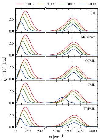
Figure 1: Simulated absorption spectra for the two-dimensional OH-bond model. The curvilinear centroids used in QCMD yield good agreement with the exact quantum (QM) and Matsubara-dynamics spectra, whereas the cartesian centroids used in CMD artificially red-shift and broaden the OH-stretch bands. The QCMD results were calculated as described in Sec. II; all other results are taken from ref. 38.

We further simplify the calculation of the force by making the approximation

$$-\dfrac{\partial\overline{F}(R)}{\partial\overline{\bf Q}}\simeq-\left\langle\dfrac{\partial U(\mathbf{q})}{\partial\overline{\bf Q}}\right\rangle_{R}$$ (18)

where

$$\left\langle\dots\right\rangle_{R} =\dfrac{1}{{\overline{Z}}_{0}(R)}\int d{\bf q}^{\prime}e^{-\beta W({\bf q}^{\prime})}(\ldots)\,\delta\!\left(R^{\prime}-R\right),$$ (19)

which is equivalent to assuming that the polymer-spring forces do not survive the mean-field averaging.Jacob Unlike its counterpart in CMD, Eq. (18) is not exact, since $R$ contains components of the ring-polymer normal modes orthogonal to the centroid. However, the size of this spring-force will depend on the extent to which the ring-polymer distribution spreads and contracts as a function of $R$, and is thus expected to be small if the distribution remains compact. The advantage of Eq. (18) is that it will allow us later (Sec. IV) to evaluate the force on-the-fly using a simple algorithm. The cartesian forces of Eq. (18) are obtained from the forces on $R$ using

$$-\dfrac{\partial U(\mathbf{q})}{\partial\overline{\bf Q}} =\dfrac{\overline{\bf Q}}{R}f_{R}(\mathbf{q})$$ (20)

with

$$f_{R}(\mathbf{q}) \equiv-\dfrac{\partial U(\mathbf{q})}{\partial R}=-\dfrac{1}{N}\sum_{i=1}^{N}\dfrac{\mathbf{q}_{i}}{r_{i}}\!\cdot\!\bm{\nabla}V(\mathbf{q}_{i}).$$ (21)

Having propagated the quasi-centroid trajectory $\overline{Q}(t)$, the spectrum is then obtained from the time-correlation function

$$\overline{C}(t) =\dfrac{1}{(2\pi\hbar)^{2}\overline{Z}}\int\!d\overline{\mathbf{P}}\int\!d\overline{\bf Q}\,e^{-\beta\overline{H}(\overline{\bf P},\overline{\bf Q})}\,\dot{\bm{\mu}}(\overline{\mathbf{Q}})\!\cdot\!\dot{\bm{\mu}}(\overline{\mathbf{Q}}(t))$$ (22)

with

$$\overline{Z} =\dfrac{1}{(2\pi\hbar)^{2}}\int\!d\overline{\mathbf{P}}\int\!d\overline{\mathbf{Q}}\,e^{-\beta\overline{H}(\overline{\mathbf{P}},\overline{\mathbf{Q}})}$$ (23)

and

$$\overline{H}(\overline{\bf P},\overline{\bf Q})=\overline{\bf P}^{2\!}/2m+f(\overline{\mathbf{Q}})$$ (24)

where $f(\overline{\mathbf{Q}})\simeq\overline{F}(\overline{\mathbf{Q}})$ is defined to be the free energy obtained by doing work with the approximate force of Eq. (18).

In a QCMD simulation, one propagates trajectories using Eqs. (15) and (18), applying a standard thermostat in order to sample the distribution $\exp(-\beta\overline{H}(\overline{\bf P},\overline{\bf Q}))$. As already mentioned, this distribution involves approximations to the exact quantum Boltzmann distribution which would not have been made in the analogous CMD calculation. In addition, CMD has the advantage of using the exact estimator for the linear dipole moment operator ${\bm{\mu}}={\bf Q}$, whereas QCMD uses the approximation ${\bm{\mu}}\simeq\overline{\bf Q}$. We thus expect QCMD to be less accurate than CMD when the temperature is high enough to neglect the curvature problem, but more accurate at lower temperatures, where the better treatment by QCMD of the dynamics will far outweigh the errors in the Boltzmann distribution which are expected to be small (provided the ring-polymer distribution is compact—see Appendix B). To be safe, we can monitor the errors in the distribution numerically, by comparing QCMD static properties with results from standard path-integral molecular dynamics (PIMD) calculations.

We tested QCMD on the two-dimensional OH-bond model of Appendix A. The forces in Eq. (21) were evaluated at 128 grid-points along the $R$ coordinate, using standard PIMDtuckerman with the quasi-centroid constraint imposed using SHAKE and RATTLE.ryckaerts ; andersen ; tuckerman The resulting spectra (Fig. 1) are in excellent agreement with the exact quantum and Matsubara results, at all temperatures tested, with no sign of a curvature problem. Figure 2 makes a closer comparison of the QCMD OH-stretch bands with the mean-field Matsubara results of ref. 38. We see that the QCMD OH-stretch peaks have small ($\sim\!10~{}\mathrm{cm}^{-1}$) blue shifts with respect to the Matsubara peaks. The shifts change slightly with temperature, ranging from $14~{}\mathrm{cm}^{-1}$ at $800~{}\mathrm{K}$ to $6~{}\mathrm{cm}^{-1}$ at $200~{}\mathrm{K}$. This variation appears to be the result of small differences in lineshape, rather than an underlying curvature problem; part of these differences may be the result of convergence artefacts in the Matsubara results.

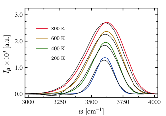
Figure 2: A closer look at the QCMD (coloured lines) and Matsubara (black lines) spectra of Fig. 1 in the region of the OH stretch band.

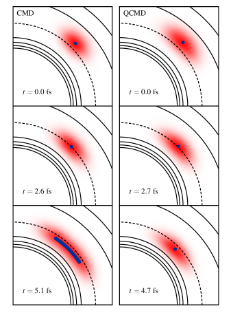
Figure 3: Snapshots of the CMD and QCMD ring-polymer bead distributions (red), along a pair of trajectories with extremely short (but thermally accessible) inner turning points, taken from the 200 K OH-model simulations. At the inner turning point (bottom), the CMD distribution fluctuates around an artificial instanton (blue blobs), whereas the QCMD distribution fluctuates around a point. The dashed contour indicates the equilibrium bond-length $r_{\mathrm{eq}}$, and the solid black contours are drawn at energy increments of $0.2D_{0}$.

As expected, the QCMD distributions contain no artificial instantons at the inner turning points (see Fig. 3). Detailed comparison with CMD trajectories is difficult (since the dynamics are different), but it appears that the QCMD distributions are broader than the CMD distributions at the outer turning points. This property may perhaps be responsible for the small blue shifts in comparison with the Matsubara results (see Fig. 2)—although if this were case, one would expect a systematic temperature dependence. Overall, the widths of the QCMD distributions vary little over a vibrational period, confirming that dynamics of the quasi-centroid is coupled only weakly to the internal degrees of freedom, so that the neglect of the ring-polymer springs in Eq. (18) is justified.

Given the excellent agreement of the QCMD and Matsubara spectra, we expect that the various QCMD static approximations mentioned above are small. This is confirmed by comparing QCMD static averages with the results of exact quantum calculations. We found that the QCMD expectation values of the bond-length $R$ were identical to within sampling error to the exact values, at all temperatures tested, and that the largest error in the $t=0$ limit of the dipole autocorrelation function was 2$\%$ at 200 K. Note that this error does not affect the calculated spectra, since these were obtained from the dipole-derivative autocorrelation function, for which QCMD gives the exact $t=0$ limit for a linear dipole.

We attempted to ‘break’ the QCMD calculations by pushing the temperature down to 50 K. However, even at this low temperature, the ring-polymer distribution around the centroid remained compact, and the agreement of QCMD with the exact quantum spectrum was as close as that shown at higher temperatures in Fig. 1. This suggests that QCMD continues to gives a good approximation to Matsubara dynamics down to 50 K (where we were unable to compute the Matsubara spectrum because the phase problem was too severe).

In summary, QCMD behaves extremely well for the two-dimensional OH model. It eliminates the curvature problem, giving spectra that lie almost on top of the Matsubara results at all temperatures tested. The errors from the ‘extra’ approximations (that $\overline{\bf P}$ is cartesian and that the polymer springs can be neglected in the force) are found to be insignificant.

III Extension to gas-phase water

We now test whether these advantages continue when QCMD is extended to treat gas-phase water. By analogy with Sec. II, we choose a set of curvilinear centroid coordinates that can be expected to give compact mean-field distributions, namely the bond-angle centroids

$$R_{1} =\dfrac{1}{N}\sum_{i}r_{i1}, r_{i1} =|\mathbf{q}^{\scriptscriptstyle{(\mathrm{OH}_{1})}}_{i}|$$

$$R_{2} =\dfrac{1}{N}\sum_{i}r_{i2}, r_{i2} =|\mathbf{q}^{\scriptscriptstyle{(\mathrm{OH}_{2})}}_{i}|$$

$$\Theta =\dfrac{1}{N}\sum_{i}\theta_{i}, \theta_{i} =\arccos\!\left[\dfrac{\mathbf{q}^{\scriptscriptstyle{(\mathrm{OH}_{1})}}_{i}\!\cdot\!\mathbf{q}^{\scriptscriptstyle{(\mathrm{OH}_{2})}}_{i}}{r_{i1}r_{i2}}\right]$$ (25)

in which $\mathbf{q}^{\scriptscriptstyle{(\mathrm{OH}_{1,2})}}_{i}={\bf q}^{\scriptscriptstyle{(\mathrm{H}_{1,2})}}_{i}\!-{\bf q}^{\scriptscriptstyle{(\mathrm{O})}}_{i}$​ are the displacement vectors between the oxygen and hydrogen atoms in the $i$-th water molecule replica ($i=1\ldots N$). A further six coordinates would be required to orient the mean-field-averaged water molecule and locate its centre-of-mass, but, like $\Theta$ in Sec. II, these external coordinates need not be specified, since no force or torque acts on them.

As in Sec. II, we carry out dynamics using equations of motion which have the same form as CMD, namely

$$\dot{\overline{\bf Q}}^{(\alpha)} =\dfrac{\overline{\bf P}^{(\alpha)}}{m_{\alpha}}$$

$$\dot{\overline{\bf P}}^{(\alpha)} =-\dfrac{\partial\overline{F}(\bm{\xi})}{\partial\overline{\bf Q}^{(\alpha)}}$$ (26)

where ${\overline{\bf Q}}^{(\alpha)}$ locate the quasi-centroids of atoms $\alpha=({\rm H}_{1},{\rm H}_{2},{\rm O})$ in the mean-field averaged water molecule. As in Sec. II, the curvilinear coordinates enter only through the force, which, by analogy with Eq. (18), is approximated as

$$-\dfrac{\partial\overline{F}(\bm{\xi})}{\partial\overline{\bf Q}^{(\alpha)}}\simeq-\left\langle\dfrac{\partial U(\mathbf{q})}{\partial\overline{\bf Q}^{(\alpha)}}\right\rangle_{\mathrlap{\!\!\bm{\xi}}}.$$ (27)

where

$$\left\langle\ldots\right\rangle_{\bm{\xi}} =\dfrac{1}{\overline{z}_{0}({\bf\xi})}\int d\mathbf{q}^{\prime}e^{-\beta W(\mathbf{q}^{\prime})}(\ldots)\,\prod_{\mathclap{\nu=1}}^{3}\delta\left(\xi_{\nu}^{\prime}-\xi_{\nu}\right)$$

$${\overline{z}}_{0}({\bm{\xi}}) =\int d\mathbf{q}^{\prime}e^{-\beta W(\mathbf{q}^{\prime})}\,\prod_{\mathclap{\nu=1}}^{3}\delta\left(\xi_{\nu}^{\prime}-\xi_{\nu}\right),$$ (28)

with $\bm{\xi}\equiv\left(\xi_{1},\xi_{2},\xi_{3}\right)\equiv\left(R_{1},R_{2},\Theta\right)$, and ${\bf q}\equiv\left\{{\bf q}_{i}^{(\alpha)}\right\}$.

The right-hand side of Eq. (27) is computed using

$$-\dfrac{\partial U(\mathbf{q})}{\partial\overline{\bf Q}^{\scriptscriptstyle{(\mathrm{H}_{k})}}}={} \dfrac{\overline{\bf Q}^{\scriptscriptstyle{(\mathrm{OH}_{k})}}}{R_{k}}f_{\!R_{k}}\!(\mathbf{q})-{}$$

$${}\dfrac{1}{R_{k}\sin\Theta} \left(\dfrac{\overline{\bf Q}^{\scriptscriptstyle{(\mathrm{OH}_{j})}}}{R_{j}}-\dfrac{\overline{\bf Q}^{\scriptscriptstyle{(\mathrm{OH}_{k})}}}{R_{k}}\cos\Theta\right)\!f_{\Theta}(\mathbf{q})$$

$$\vphantom{\dfrac{\overline{Q}^{\scriptscriptstyle{(\mathrm{OH}_{k})}}_{\nu}}{R_{k}}}-\dfrac{\partial U(\mathbf{q})}{\partial\overline{\bf Q}^{\scriptscriptstyle{(\mathrm{O})}}}={} \sum_{k=1,2}\dfrac{\partial U(\mathbf{q})}{\partial\overline{\bf Q}^{\scriptscriptstyle{(\mathrm{H}_{k})}}},$$ (29)

with $(k,j)=(1,2)$ or $(2,1)$, and

$$f_{R_{k}}\!(\mathbf{q}) \equiv-\dfrac{\partial U(\mathbf{q})}{\partial R_{k}}=-\dfrac{1}{N}\sum_{i=1}^{N}\dfrac{\mathbf{q}^{\scriptscriptstyle{(\mathrm{OH}_{k})}}_{i}}{r_{ik}}\cdot\!\bm{\nabla}_{\!\mathrm{H}_{k}\!}V(\mathbf{q}_{i})$$

$$f_{\Theta}(\mathbf{q})\equiv -\dfrac{\partial U(\mathbf{q})}{\partial\Theta}=\dfrac{1}{N}\sum_{i=1}^{N}\dfrac{r_{i1}}{\sin\theta_{i}}\times$$

$$\left(\dfrac{\mathbf{q}^{\scriptscriptstyle{(\mathrm{OH}_{2})}}_{i}}{r_{i2}}-\dfrac{\mathbf{q}^{\scriptscriptstyle{(\mathrm{OH}_{1})}}_{i}}{r_{i1}}\cos\theta_{i}\right)\cdot\bm{\nabla}_{\!\mathrm{H}_{1}\!}V(\mathbf{q}_{i}),$$ (30)

where $\bm{\nabla}_{\!\mathrm{H}_{k}\!}V(\mathbf{q}_{i})$ is the force on the $i$-th bead of the $k$-th hydrogen. The infrared spectrum is obtained from

$$\overline{C}_{\mu\mu}(t)=\dfrac{1}{(2\pi\hbar)^{9}\overline{Z}}\int\!d\overline{\mathbf{P}}\!\int\! d\overline{\mathbf{Q}}\,e^{-\beta\overline{H}(\overline{\bf P},\overline{\bf Q})}$$

$$\times\bm{\mu}(\overline{\mathbf{Q}})\!\cdot\!\bm{\mu}(\overline{\mathbf{Q}}(t)),$$ (31)

with

$$\overline{H}(\overline{\bf P},\overline{\bf Q}) =\sum_{\alpha}\left[\overline{\mathbf{P}}^{(\alpha)}\right]^{\mathrlap{2}\,}/2m_{\alpha}+f(\overline{\mathbf{Q}})$$ (32)

where $f(\overline{\mathbf{Q}})\simeq\overline{F}(\overline{\mathbf{Q}})$ is the free energy obtained by doing work with the approximate force of Eq. (27).

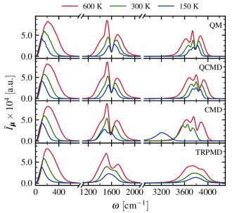
Figure 4: Simulated rovibrational absorption spectra for gas-phase water, obtained after damping the time-correlation function with a Hann window of width $\tau=750~{}$\mathrm{f}\mathrm{s}$$. The QCMD results were calculated using the bond-angle centroids of Sec. III, and show good agreement with the exact quantum results (QM), with no sign of the red shift and broadening seen in the CMD stretch. The absorption intensities are scaled by a factor of 4.5 for $\omega>1200~{}\mathrm{cm}^{-1}$.

We used the above framework to simulate QCMD infrared spectra for gas-phase water using the Partridge-Schwenke potential surfacepspes and dipole moment.psdms As in Sec. II, we damped the time-correlation functions before calculating their Fourier transform, this time using a Hann windownr77 of 750 $\mathrm{f}\mathrm{s}$. The quasi-centroid forces in Eq. (30) were calculated on a $64\times 64\times 64$ grid, using standard PIMDtuckerman with SHAKE/RATTLE to impose the quasi-centroid constraints,ryckaerts ; andersen ; tuckerman and were then fitted to cubic splines.nr77 At 600 and 300 K, the grids ranged from 1.50 to 2.50 a.u. in $R_{1,2}$ and from $85^{\circ}$ to $130^{\circ}$ in $\Theta$; at 150 K this range was reduced to 1.65 – 2.05 a.u. and $90^{\circ}$ – $126^{\circ}$. We also calculated the exact quantum spectrum (subject to the same damping) using the DVR3D package of Tennyson and co-workers,dvr3d and the corresponding CMD and TRPMD spectra using standard PIMD techniques. A comparison with Matsubara dynamics was not possible because the Matsubara sign problem was too severe.

From Fig. 4, we see that QCMD works extremely well for gas-phase water. The overall agreement with the exact quantum results is excellent, even at 150 K, where there is again no sign of a curvature problem. There are small differences between the QCMD and quantum spectra: the QCMD bend ($\sim\!1600~{}\mathrm{cm}^{-1}$) and stretch ($\sim\!3800~{}\mathrm{cm}^{-1}$) have different internal structures from those in the exact spectrum, and the stretch is blue-shifted by about $60~{}\mathrm{cm}^{-1}$. The main cause of these differences is most likely the neglect of real-time coherence by QCMD. Note that the positions of the TRPMD bands are very close to those of the QCMD bands, implying that, as expected, TRPMD gives a good description of the short-time dynamics of gas-phase water.

As in the two-dimensional model, the gas-phase water QCMD distributions remain compact at inner turning points because there are no quasi-centroid-constrained instantons. Figure 5 compares the distributions at inner turning points of an ‘extreme’ QCMD and CMD trajectory at 150 K. As in the two-dimensional case, the QCMD distribution remains localised whereas the CMD distribution spreads around a centroid-constrained instanton. This artefact distorts the approximate axial symmetry of the distribution around the OH bond into a banana shape.

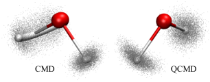
Figure 5: Ring-polymer distributions (dots) at the inner turning points of CMD and QCMD trajectories corresponding to very short (but thermally accessible) OH bond lengths, taken from the gas-phase water simulations at 200 K. The CMD distribution fluctuates around an artificial instanton (spheres), whereas the QCMD distribution fluctuates around a localised geometry.

Comparisons of the QCMD average OH bond lengths with those obtained using standard PIMD give tiny differences ($0.1\%$ at 150 K), indicating that, as for the two-dimensional model, the approximate distribution in Eq. (32) is very close to the exact quantum Boltzmann distribution. Note that, since the Partridge-Schwenke dipole moment is non-linear,psdms neither CMD nor QCMD give the exact quantum Kubo time-correlation function in the $t\to 0$ limit,hone2 ; paes2008 and that both methods neglect the Matsubara fluctuation terms necessary to completely describe the dipole-moment dynamics at low temperatures.mats ; mats-rpmd ; mf-mats

IV Implementing QCMD using an adiabatic propagator

In Sec. II and III, we applied QCMD to systems that are small enough for the mean-field force on the quasi-centroid to be pre-calculated on a grid. To apply QCMD to larger systems, we adapt the adiabatic CMD (ACMD) algorithm, used in previous workcaov4 ; hone1 ; hone2 to calculate the mean-field centroid force on-the-fly.

In ACMD, the ring polymer is represented in terms of the normal modes that diagonalise the ring-polymer spring potential. These are Fourier modes, such that for each cartesian degree of freedom the lowest frequency mode $s_{0}$ is (proportional to) the centroid.coalson The mass associated with each non-centroid mode $s_{n}$ is then scaled by a factor of $(\beta\hbar\omega_{n}/\gamma N)^{2}$, where $\omega_{n}$ is the associated normal-mode frequency, and a local thermostat is applied to its dynamics. The limit $\gamma\to\infty$ gives a perfect adiabatic separation between the motion of the centroid and the thermostatted normal modes, and is thus equivalent to CMD.hone2 In practice, $\gamma$ is treated as a convergence parameter, with e.g. $\gamma=64$ giving a good approximation to CMD in gas-phase water at 150 K.

It is straightforward to modify the ACMD algorithm to an AQCMD algorithm that adiabatically separates the motion of the quasi-centroid from that of all the other degrees of freedom. In the AQCMD algorithm, a simulation is treated as two systems evolving in parallel, one of quasi-centroids with phase-space coordinates $(\overline{\mathbf{P}},\overline{\mathbf{Q}})$, and one of ring-polymers with coordinates $(\mathbf{p},\mathbf{q})$. The dynamics is propagated using a modification of the integrator due to Leimkuhler and Matthews with OBABO operator splitting.leimkuhler A propagation step begins with the thermostatting of the momenta:

1. Propagate the quasi-centroid momenta $\overline{\mathbf{P}}$ for half a time-step ($\Delta t/2$) under the action of a Langevin thermostat.

2. Propagate the bead momenta ${\bf p}$ for $\Delta t/2$ under the path-integral Langevin equation (PILE) thermostat,pile followed by RATTLEandersen to constrain the quasi-centroid components.

The momenta are then updated according to the forces acting on the system:

1. Propagate $\overline{\bf P}$ for $\Delta t/2$ under the quasi-centroid forces.

2. Propagate $\mathbf{p}$ for $\Delta t/2$ under the forces derived from the ring-polymer potential in Eq. (5), followed by RATTLE.

This is followed by a position update:

1. Propagate the quasi-centroid positions $\overline{\mathbf{Q}}$ for a full time-step $\Delta t$ according to the current values of the momenta $\overline{\mathbf{P}}$.

2. Propagate the bead positions $\mathbf{q}$ for $\Delta t$ according to the current values of $\mathbf{p}$, followed by SHAKE,ryckaerts which constrains the ring-polymer geometry to be consistent with the quasi-centroid configuration $\overline{\mathbf{Q}}$ obtained at the end of step A1.

The propagation step is concluded by executing B1–B2 using the forces evaluated at the updated positions, followed by O1–O2. The mass-scaling used in the propagation of the ring-polymers is the same as in ACMD, except that the mass of the centroid is also scaled, by $\gamma^{-2}$. A useful feature of this algorithm is that it requires explicit forces only on the quasi-centroid (B1) and on the cartesian bead coordinates (B2), but does not require explicit forces on the degrees of freedom orthogonal to the quasi-centroid. Note that the AQCMD algorithm reduces to the ACMD algorithm in the special case that the quasi-centroid is taken to be the centroid (at which point the constraints become trivial to apply).

We tested the convergence with respect to $\gamma$ by applying the AQCMD algorithm to gas-phase water at 150 K. A value of $\gamma=64$ was sufficient to reproduce the spectrum obtained by interpolating the force on a grid. The adiabatic simulation required a time-step of $\Delta t=0.1/\gamma~{}$\mathrm{f}\mathrm{s}$$, i.e. $\gamma$ times smaller than what would have been used to propagate the dynamics without the mass scaling. We note that the same values of $\gamma$ and $\Delta t$ are required to converge ACMD at this temperature, and hence that the AQCMD algorithm uses approximately the same amount of CPU time as the ACMD algorithm, since most of the time is spent evaluating the forces on the ring-polymer beads.

In condensed phase simulations, converged ACMD results can be obtained at significantly lower adiabatic separation,hone2 ; mano-pacmd provided the strength of the thermostat acting on the non-centroid modes is carefully tuned.trpmd2-sup This approach is known as partially-adiabatic CMD (PACMD). We have not yet attempted a similar partially-adiabatic implementation of QCMD and view it as an important step in future methodological development.

V Liquid water and ice

Using the AQCMD algorithm just described, we carried out preliminary QCMD simulations of liquid water and ice, using the q-TIP4P/F potential energy and dipole moment surfaces.qtip4pf We used sets of bond-angle centroids, defined as in Eq. (25) to describe the internal motion of the water monomers, and ‘Eckart-like’ rotational frames (see Sec. V.1) to describe the translations and overall rotations of the monomers. Numerical details and results of the simulations are presented in Sec. V.2.

V.1 Eckart-like frame

V.1.1 Properties of the frame

In molecular spectroscopy, the Eckart frame defines the orientation of a molecule by means of a reference geometry, usually taken to be the equilibrium geometry.eckart ; bright-wilson Here, we orient each water monomer using an ‘Eckart-like’ frame, in which the ‘molecule’ is the monomer ring-polymer, and the ‘reference geometry’ is the monomer quasi-centroid. This gives the conditions

$$\sum_{\alpha,i}m_{\alpha}(\mathbf{q}_{i}^{(\alpha)}-\overline{\mathbf{Q}}^{(\alpha)}) =\mathbf{0}$$ (33a)

$$\sum_{\alpha,i}m_{\alpha}\overline{\mathbf{Q}}^{(\alpha)}\times(\mathbf{q}_{i}^{(\alpha)}-\overline{\mathbf{Q}}^{(\alpha)}) =\mathbf{0},$$ (33b)

where we use the notation of Sec. III, such that $\mathbf{q}_{i}^{(\alpha)}$ are the atom polymer beads and $\overline{\mathbf{Q}}^{(\alpha)}$ are the atom quasi-centroids, with $\alpha=({\rm H}_{1},{\rm H}_{2},{\rm O})$. It is easy to show that these conditions are equivalent to

$$\sum_{\alpha}m_{\alpha}(\mathbf{Q}^{(\alpha)}-\overline{\mathbf{Q}}^{(\alpha)}) =\mathbf{0}$$ (34a)

$$\sum_{\alpha}m_{\alpha}\overline{\mathbf{Q}}^{(\alpha)}\times(\mathbf{Q}^{(\alpha)}-\overline{\mathbf{Q}}^{(\alpha)}) =\mathbf{0}.$$ (34b)

where $\mathbf{Q}^{(\alpha)}$ are the atom centroids.

The first condition (Eq. (33a) or, equivalently, Eq. (34a)) thus places the centre-of-mass of the atom quasi-centroids at the centre-of-mass of the entire monomer ring-polymer, or equivalently, at the centre-of-mass of the atom centroids.

The second condition (Eq. (33b) or, equivalently, Eq. (34b)) specifies the orientation of the monomer ring-polymer about its centre-of-mass. To illustrate how this works, let us imagine that we have generated a new monomer quasi-centroid geometry $\overline{\mathbf{Q}}$ (using step A1 of the AQCMD algorithm), and that we now wish to define the ensemble of ring-polymers that ‘belong’ to this geometry. One can show that the second Eckart condition is equivalent to minimisingjorg ; kudin

$$\sum_{\alpha,i}m_{\alpha}|{\bf q}_{i}^{(\alpha)}-\overline{\mathbf{Q}}^{(\alpha)}|^{2}$$

or, equivalently,

$$\sum_{\alpha}m_{\alpha}|{\mathbf{Q}}^{(\alpha)}-\overline{\mathbf{Q}}^{(\alpha)}|^{2}$$

In other words, each monomer ring-polymer in the ensemble is oriented so as to minimise its average mass-weighted distance from $\overline{\mathbf{Q}}$. In practice, this means that the atom centroids are usually very close to the atom quasi-centroids—see Fig. 6. The Eckart-like conditions thus ensure that the quasi-centroid-constrained ring-polymer distribution is compact with respect to the orientational degrees of freedom.minsp

V.1.2 Implementation

To implement the Eckart-like conditions, we carry out the propagation in cartesian coordinates $(\overline{\mathbf{P}},\overline{\mathbf{Q}})$, using the AQCMD algorithm of Sec. IV. This allows us to avoid using Euler angles or quaternions. Steps O2, B2, and A2 of the AQCMD algorithm are straightforward to implement by imposing the constraints of Eq. (25) and Eq. (34) on each monomer using SHAKE and RATTLE.ryckaerts ; andersen ; tuckerman Step B1 is implemented as follows.

First, to take into account that there are now external forces acting on the polymer beads, the expressions for the internal forces given in Eq. (30) are modified according to

$$\bm{\nabla}_{\!\alpha}V(\mathbf{q}_{i})\to\bm{\nabla}_{\!\alpha}V(\mathbf{q}_{i})+m_{\alpha}\!\left[\dfrac{\mathbf{f}_{i}}{m_{\mathrm{tot}}}+(\mathbf{I}^{-1}_{i}\bm{\tau}_{i})\times\mathbf{q}^{(\alpha)}_{i}\right]\!$$ (35)

with

$$\mathbf{f}_{i} =-\sum_{\alpha}\dfrac{\partial V(\mathbf{q})}{\partial\mathbf{q}^{(\alpha)}_{i}}$$ (36)

$$\bm{\tau}_{i} =-\sum_{\alpha}\left(\mathbf{q}^{(\alpha)}_{i}-\mathbf{q}^{({\rm c})}_{i}\right)\times\dfrac{\partial V(\mathbf{q})}{\partial\mathbf{q}^{(\alpha)}_{i}},$$ (37)

where $\mathbf{q}_{i}^{(c)}$ is the centre-of-mass of the $i$-th replica, and $\mathbf{I}_{i}$ is its inertia tensor in the centre-of-mass frame. Having made this modification, we use Eqs. (29) and (30) to compute the internal forces on the quasi-centroid.

Second, we add the external forces on the monomer quasi-centroids, which are given by

$$-\left.\dfrac{\partial U(\mathbf{q})}{\partial\overline{\mathbf{Q}}^{(\alpha)}}\right|_{\mathrlap{\mathrm{ext}}}=m_{\alpha}\!\left[\dfrac{\overline{\mathbf{f}}}{m_{\mathrm{tot}}}+\left(\mathbf{I}^{-1}\overline{\bm{\tau}}\right)\times\overline{\mathbf{Q}}^{(\alpha)}\right],$$ (38)

where

$$\overline{\mathbf{f}} =-\sum_{\alpha}\dfrac{\partial U(\mathbf{q})}{\partial\overline{\mathbf{Q}}^{(\alpha)}}$$

$$\overline{\bm{\tau}} =-\sum_{\alpha}\left(\overline{\mathbf{Q}}^{(\alpha)}-\overline{\mathbf{Q}}^{({\rm c})}\right)\times\dfrac{\partial U(\mathbf{q})}{\partial\overline{\mathbf{Q}}^{(\alpha)}}$$ (39)

with $\overline{\mathbf{Q}}^{(c)}$ the quasi-centroid centre-of-mass and $\mathbf{I}$ the quasi-centroid inertia tensor. The centre-of-mass force $\overline{\mathbf{f}}$ is easy to compute since it is just the average of the forces on the replica centres-of-mass

$$\overline{\mathbf{f}} =\dfrac{1}{N}\!\sum_{i}\mathbf{f}_{i}$$ (40)

but the torque $\overline{\bm{\tau}}$ is difficult to compute exactly.invert We therefore approximate $\overline{\bm{\tau}}$ as the average of the torques on the replicas

$$\overline{\bm{\tau}}\simeq\dfrac{1}{N}\sum_{i}{\bm{\tau}}_{i}$$ (41)

This expression is consistent with the other approximations made to the forces (namely that $\overline{\bf P}$ is purely cartesian, and that the polymer springs can be neglected in the mean-field force), since Eqs. (39) and (41) agree to within second order in the displacements from the quasi-centroid. As with these other approximations, the reliability of Eq. (41) can be monitored by comparing QCMD static properties with the results of standard PIMD simulations.

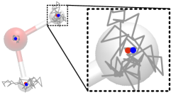
Figure 6: A typical ring-polymer geometry from a QCMD water simulation at 150 K, showing how the Eckart-like conditions have oriented the polymer such that the atom centroids (red) almost coincide with the atom quasi-centroids (blue).

V.2 Simulation results

V.2.1 Computational details

Condensed-phase water CMD, TRPMD and QCMD simulations were carried out in the three regimes studied in ref. 35, namely the compressed liquid at $600~{}$\mathrm{K}$$, the liquid at $300~{}$\mathrm{K}$$, and ice I_h at $150~{}$\mathrm{K}$$.

Unless noted otherwise, the CMD and TRPMD calculations used the same parameters as ref. 35, with periodic boundary conditionsfrenkel ; allen and simulation boxes of 128 molecules for the liquid and 96 for ice. At each temperature, a set of independent starting configurations was generated by propagating eight instances of the system classically for $100~{}$\mathrm{p}\mathrm{s}$$ under the action of a global Langevin thermostat,schneider-langevin ; bussi-langevin followed by a $100~{}$\mathrm{p}\mathrm{s}$$ TRPMD run under PILE-G (with the centroid relaxation time $\tau_{0}=100~{}$\mathrm{f}\mathrm{s}$$, and the non-centroid mode friction parameter $\lambda=0.5$).pile The resulting eight equilibrated ring-polymer configurations were then propagated for a further $100~{}$\mathrm{p}\mathrm{s}$$, using PILE-G (with the same parameters as above) to give the TRPMD results, and the PA-CMD algorithm (with $\gamma=4$, $\tau_{0}=100~{}\mathrm{fs}$, and $\lambda=0.01$) to give the CMD results.

To compute the QCMD spectra for the liquid, we took the eight equilibrated configurations obtained after the first 100 ps PILE-G (see above), then propagated for $35~{}$\mathrm{p}\mathrm{s}$$ using the AQCMD algorithm as described in Sec. IV and V.1, with a global Langevin thermostatbussi-langevin (time constant $\tau_{0}=100~{}$\mathrm{f}\mathrm{s}$$) acting on the quasi-centroids. The first $10~{}$\mathrm{p}\mathrm{s}$$ were discarded before calculating the dipole-derivative time-correlation functions.

For QCMD ice, we generated 15 independent equilibrated configurations (in the same manner as the 8 in the liquid simulations). These were then propagated with the AQCMD algorithm for $2.5~{}$\mathrm{p}\mathrm{s}$$, with a local Langevin thermostatbussi-langevin acting on the quasi-centroids. For each of the 15 configurations, the system was then propagated under a global Langevin thermostatbussi-langevin for three intervals of $2.5~{}$\mathrm{p}\mathrm{s}$$, separated by relaxation periods of $300~{}$\mathrm{f}\mathrm{s}$$, during which local thermostatting was used. The IR spectrum was then calculated by averaging over the three $2.5~{}$\mathrm{p}\mathrm{s}$$ trajectories from the 15 independent simulations. Converged AQCMD results were obtained using $\gamma=8$ at 600 K, and $\gamma=32$ at 300 K. At 150 K, the calculation was stopped at $\gamma=128$, which has definitely converged the positions of the peaks and the $t\to 0$ limit of the dipole-derivative time-correlation function, but may not yet have converged the intensity of the stretch peak—see Appendix C. These values of $\gamma$ made the QCMD calculations approximately $2,\,8,\,\text{and}\ 32$ times more expensive than the corresponding CMD calculations, which used the PA algorithmhone2 ; mano-pacmd and thus smaller values of $\gamma$.

V.2.2 Overview of the QCMD spectrum

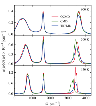
Figure 7: Simulated infrared absorption spectra for q-TIP4P/F water, at 600 K (compressed liquid), 300 K (liquid), and 150 K (ice I_h), obtained by damping the time-correlation function with a Hann window of width $\tau=600~{}$\mathrm{f}\mathrm{s}$$ at 600 and 300 K, and $\tau=800~{}$\mathrm{f}\mathrm{s}$$ at 150 K. The bond-angle centroids used in the QCMD simulations appear to have eliminated the red-shifts and broadening seen in the CMD stretch band at 300 and 150 K.

At 600 K, the QCMD spectra are in very close agreement with the TRPMD and CMD spectra (Fig. 7). Measured from the peak maximum, the QCMD OH stretch at $3600~{}\mathrm{cm}^{-1}$ is blue-shifted by about $15~{}\mathrm{cm}^{-1}$ relative to CMD and TRPMD. The bend at $1600~{}\mathrm{cm}^{-1}$ and the libration peak at $500~{}\mathrm{cm}^{-1}$ are almost identical in all three methods.

At 300 K, noticeable differences emerge between QCMD and the other two methods, due to the CMD curvature problem, and the broadening of TRPMD, although these problems are a lot less severe than in the gas-phase at this temperature.marx10 ; trpmd2 The CMD stretch peak is red-shifted relative to TRPMD by about $50~{}\mathrm{cm}^{-1}$; the QCMD stretch peak is blue-shifted by about $20~{}\mathrm{cm}^{-1}$. The bend peaks are in good agreement for all three methods. The libration band in QCMD is slightly red-shifted; the most possible cause for this small shift is the approximation made to the torques on the monomers in Eq. (41) (see Sec. V.2.4).

In $150~{}$\mathrm{K}$$ ice, there are major differences between the three sets of results, mainly in the stretch region. The curvature problem is strong, artificially broadening and red-shifting the CMD stretch by more than $100~{}\mathrm{cm}^{-1}$, and the TRPMD stretch is severely broadened. In contrast, the QCMD stretch is sharp, with resolved symmetric and antisymmetric bands. This resolution of the stretch bands is an artefact of the q-TIP4P/F surface and is also observed in classical simulations. Using a shorter time window of 500 $\mathrm{f}\mathrm{s}$ to coalesce the QCMD stretch peaks (not shown), gives a QCMD stretch that is blue-shifted by about $10~{}\mathrm{cm}^{-1}$ with respect to the TRPMD stretch, and is more than twice as intense. Note that (as mentioned above) the intensity of the QCMD stretch may not have converged with respect to $\gamma$. All three methods are in close agreement in the libration and bend regions, with a slight red-shift in the QCMD libration band which is smaller than the shift at 300 K (see Sec. V.2.4).

V.2.3 Stretch region of the QCMD infrared spectrum

To better assess the performance of QCMD in the stretch region of the spectrum ($>2000$ cm^-1), we compare with two other methods: the coloured-noise version of TPRMD developed recently by Rossi et al.trpmd3 and the local monomer approximation (LMon) of Bowman and co-workers.lmon1 ; lmon2 ; trpmd2 Both methods are expected to do well in the stretch region of the spectrum, but to suffer from artefacts at lower frequencies.

In coloured-noise TRPMD, the white-noise PILE thermostat used in most TRPMD calculations (such as those reported above) is replaced by a generalised Langevin equation (GLE) thermostat that is designed to minimise the dynamical disturbance to the centroids at certain pre-tuned frequencies.trpmd3 Using the GLE(C) parametrisation of the thermostat in ref. trpmd3, (along with the other simulation parameters in this reference), we propagated eight independent 100 $\mathrm{p}\mathrm{s}$ TRPMD+GLE(C) trajectories at 300 and 150 K, using the i-PI package.ipi The resulting spectra in the stretch-region are shown in Fig. 8; (the lower-frequency parts of the spectrum, which are corrupted by the thermostat, are shown in Appendix D).

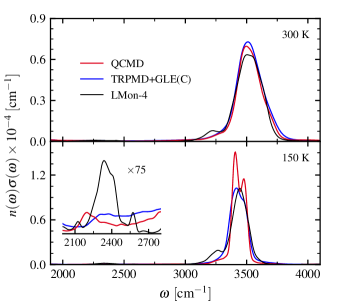
Figure 8: The stretch region of the infrared absorption spectra from the same QCMD simulations as Fig. 7, compared with TRPMD+GLE(C) spectra calculated as in ref. 36, and LMon-4 spectra taken from ref. 35. The inset magnifies the combination-band part of the spectrum.

In the LMon method, the solid or liquid is equilibrated using standard PIMD techniques, then the Schrödinger equation for the nuclear dynamics is solved for each monomer independently, with all degrees of freedom except for the internal and few intramolecular modes of the monomer held fixed.lmon1 ; lmon2 ; lmon3 ; lmon4 Here, we make use of the results of previous LMon calculations,trpmd2 in which the PIMD equilibration was done using the same box size and simulation parameters as in the TRPMD calculations of Sec. V.2.1, and the internal modes of the water molecule were coupled to each of its three librational modes in turn, resulting in a four-mode approximation (LMon-4). We convolved the raw data obtained from these calculationsmariana with the same time-windows as used in the QCMD calculations (see Appendix A), to obtain the spectra shown in Fig. 8 for the stretch region at 300 and 150 K. The approximate treatment of the intermolecular modes means that LMon-4 gives a relatively poor description of the spectrum at 600 K (not shown) and of the libration at all temperatures (see Appendix D).

The agreement between the QCMD and TRPMD+GLE(C) stretch peaks is excellent: at 300 K the peaks are almost identical; at 150 K the TRPMD+GLE(C) peaks line up with the QCMD peaks, but are somewhat broader, with the bifurcation just visible; (the broadening is to be expected since the thermostat couples more strongly to the centroid at lower temperatures). There is probably some cancellation of errors between these two sets of results, as the QCMD method makes a number of static approximations (see Sec. II.2), and the GLE(C) thermostat interferes strongly with the dynamics of the librational modes which are coupled to the dynamics of the stretch modes. One piece of evidence for such errors is that the 300 K QCMD peak is slightly less intense than the TRPMD+GLE(C) peak, whereas one would expect the opposite to be true. Nonetheless the agreement between QCMD and TRPMD+GLE(C) in the stretch region is remarkable, suggesting that both methods give excellent approximations to the Matsubara-dynamics spectrum in this region.

The QCMD and LMon-4 results are also in good agreement in the stretch region (Fig. 8). Clearly one cannot use LMon-4 as a quantum benchmark, since it includes only a few degrees of freedom in the monomer dynamics (which is probably why it does not reproduce the bifurcation in the stretch peak). Nevertheless, we think the comparison in Fig. 8 highlights an important weaknesses in the QCMD approach (which is shared by CMDpaesnew and TRPMDtrpmd2 ). The LMon-4 spectrum gives a libration-bend combination band at roughly $2300~{}\mathrm{cm}^{-1}$ (see the Fig. 8 inset) and a Fermi resonance overlapping with the stretch peak at $3200~{}\mathrm{cm}^{-1}$; both these features are much more intense than the corresponding features in the QCMD, CMD and TRPMD spectra. While we cannot say how well the LMon-4 calculations have converged these features, it seems highly likely that QCMD, CMD and TRPMD grossly underestimate them. This is not surprising, as we expect such features to depend strongly on Matsubara fluctuations,mats ; mats-rpmd and also probably on real-time coherence—effects which QCMD, CMD and TRPMD omit.

V.2.4 Approximations to the quantum Boltzmann distribution

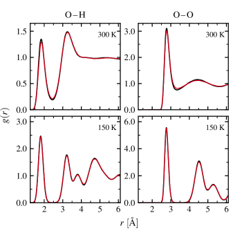
Figure 9: Simulated oxygen-hydrogen (O-H) and oxygen-oxygen (O-O) radial distribution functions (RDFs) for q-TIP4P/F water, calculated using QCMD (red) and standard PIMD (black). Hydrogen-hydrogen RDFs (not shown) are in similarly close agreement. The QCMD results are given for an adiabatic separation of $\gamma=64$ at $300~{}$\mathrm{K}$$ and $\gamma=128$ at $150~{}$\mathrm{K}$$. Only the intermolecular part of the distribution is shown for O-H; the intramolecular distributions obtained using the two methods agree to within graphical accuracy.

On the basis of the spectra reported above, it seems likely that QCMD gives a similarly good approximation to the quantum Boltzmann distribution for the condensed phase as it does for the two-dimensional model and the gas-phase. However, the condensed-phase QCMD calculations make extra approximations to the quantum Boltzmann distribution: Eq. (41) approximates the torques on the monomers, and the AQCMD algorithm only samples the exact quantum Boltzmann distribution in the limit $\gamma\to\infty$.

To test these static approximations, we compare (in Fig. 9) the AQCMD radial distribution functions (RDFs) for the liquid at 300 K and ice at 150 K with the exact RDFs (obtained from PIMD). As expected, the AQCMD RDFs are close to the exact values, although there are small errors at 300 K, indicating that AQCMD gives a slightly less structured liquid than it should. Given that the AQCMD RDFs are in almost perfect agreement with the exact values for 150 K ice, and that the intramolecular peaks in the O–H RDF (not shown) agree to graphical accuracy, we think that the (small) errors at 300 K are mainly the result of approximating the monomer torques by Eq. (41). There is perhaps also a very small contribution to the errors from incomplete convergence in $\gamma$; increasing $\gamma$ from 32 to 64 reduced slightly the errors in the RDFs, suggesting that higher values of $\gamma$ might reduce them further.

These results suggest that QCMD gives an excellent approximation to the quantum Boltzmann distributions in water and ice, except for small errors in the long-range correlations at 300 K, which are most likely due to the quasi-centroid torque estimator of Eq. (41). This estimator is also thought to be responsible for the small red shift in the libration band of the infrared spectrum at 300 K (see Fig. 7). Future work may thus be able to reduce both of these (small) errors, by developing better torque estimators.

VI Conclusions

By making minor approximations to the quantum Boltzmann distribution, we have obtained a method (QCMD) for propagating curvilinear mean-field centroids which is at least efficient enough to treat liquid water and ice on the q-TIP4P/F potential. For a two-dimensional model, the quantum Boltzmann approximations are found to be almost exact, and the infrared spectrum is close to that obtained from Matsubara dynamics, showing no sign of the ‘curvature problem’ that afflicts CMD at low temperatures. For liquid water (300 K) and ice (150 K), the errors made in the quantum Boltzmann approximations are found to be small, suggesting that the QCMD spectra are also very close to the Matsubara-dynamics spectra for these systems. The algorithm we developed to implement QCMD is slow (taking 32 times longer than PA-CMD for 150 K ice), but is do-able, and we hope to apply it soon to more realistic water potentials such as MB-pol, to allow comparison with experiment. It may be possible to speed up the algorithm by making it partially adiabatic, or perhaps to develop instead a curvilinear version of TRPMD.

As with other ring-polymer dynamics methods, such as CMD and (T)RPMD, QCMD is a (quasi-)centroid-following method, and thus cannot obtain information about the dynamics of the Matsubara fluctuations around the centroid. In general, QCMD will thus give poor results for non-linear operators waterpole (which depend explicitly on the dynamics of the Matsubara fluctuation modes), and for overtones and combination bands (which couple the centroid strongly to the fluctuation modes)—as an example of the latter, see Fig. 8.

How readily can QCMD be generalised to systems other than water? This question is equivalent to asking how readily collective bead coordinates can be identified, around which the ring-polymers are distributed compactly. Such coordinates are probably easy to find for liquids and solids made up of small, rigid molecules; but further work will be required to determine whether they can be found for systems containing floppy molecular units, such as solvated protons. Also, for reaction barriers below the instanton cross-over temperature, the collective bead coordinates will need to include the unstable mode of the instanton. A ‘holy grail’ would be to develop an algorithm that follows, automatically, the collective bead coordinate that minimises the spread of the ring-polymer distribution, thus giving the best mean-field approximation to Matsubara dynamics.

Appendix A Details of the calculations of the infrared absorption spectra

The champagne-bottle potential used in Sec. II is

$$V(r)=D_{0}\left[1-e^{-\alpha(r-r_{\mathrm{eq}})}\right]^{2},$$ (42)

where $r=\big{(}q_{x}^{2}+q_{y}^{2}\big{)}^{1/2},\,r_{\mathrm{eq}}=1.8324$, $D_{0}=0.18748$, and $\alpha=1.1605$ a.u. The mass of the particle is taken to be $m=1741.1$ a.u.

For the linear dipole-moment calculations (i.e. the 2D model and the condensed-phase water calculations), the infrared spectrum was obtained from the Kubo-transformed time-autocorrelation function (TAF) $C(t)$ of the cell dipole-moment derivative $\dot{\bm{\mu}}$tfmiller1 ; mano-pacmd

$${\tilde{I}_{\dot{\bm{\mu}}}(\omega)=\int_{-\infty}^{\infty}\!dt\,e^{-i\omega t}C_{\dot{\bm{\mu}}\cdot\dot{\bm{\mu}}}(t)f(t)}$$

$${n(\omega)\sigma(\omega)=\dfrac{\beta}{6cV\!\epsilon_{0}}\tilde{I}_{\dot{\bm{\mu}}}(\omega),}$$ (43)

where $V$ is the cell volume, $n(\omega)$ is the refractive index, $\sigma(\omega)$ is the absorption cross-section, and $f(t)$ is a window function that dampens the tail of the TAF, reducing the ringing artefacts.nr77 For the gas-phase water calculations (which employed the Partridge-Schwenke dipole-moment surface), we used the dipole TAF

$${\tilde{I}_{\bm{\mu}}(\omega)=\int_{-\infty}^{\infty}\!dt\,e^{-i\omega t}C_{\bm{\mu}\cdot\bm{\mu}}(t)f(t)}$$

$${n(\omega)\sigma(\omega)=\dfrac{\beta}{6cV\!\epsilon_{0}}\,\omega^{2}\tilde{I}_{\bm{\mu}}(\omega).}$$ (44)

In two-dimensional and gas-phase calculations, where the cell volume $V$ is not defined, we take $\tilde{I}_{\dot{\bm{\mu}}}(\omega)$ or $\omega^{2}\tilde{I}_{{\bm{\mu}}}(\omega)$ to be “the spectrum” instead of $n(\omega)\sigma(\omega)$.

When applied to the exact quantum TAF, the damping envelope $f(t)$ serves the additional purpose of removing the recurrences that are caused by the real-time quantum coherence. In the two-dimensional model, the recurrences are well separated from the initial part of the TAF, allowing a sigmoid window with a sharp cut-off to be used,

$$f(t)=\dfrac{1}{1+e^{(|t|-t_{1/2})/\tau}},$$ (45)

with parameters $t_{1/2}=400~{}$\mathrm{f}\mathrm{s}$,\,\text{and}\ \tau=25~{}$\mathrm{f}\mathrm{s}$$. In simulations of gaseous and condensed-phase water (Sec. III and V.2) the Hann windownr77

$$f(t)=\begin{cases}\cos^{2}\!\left(\frac{\pi t}{2\tau}\right)&|t|\leq\tau\\ 0&|t|>\tau\end{cases}$$ (46)

is found to be more suitable. The cut-off time $\tau$ is set to 600 $\mathrm{f}\mathrm{s}$ for liquid water at 600 and 300 $\mathrm{K}$, and to 800 $\mathrm{f}\mathrm{s}$ for ice at 150 $\mathrm{K}$.

To obtain smooth LMon-4 spectra, for which the raw datamariana are a list of discrete transition frequencies $\{\omega_{i}\}$, we calculate

$$n(\omega)\sigma(\omega)\propto\sum_{i}\mu_{i}\tilde{f}(\omega-\omega_{i})$$

$$\tilde{f}(\omega)=\dfrac{\sin(\omega\tau)}{\omega[1-(\omega\tau/\pi)^{2}]},$$ (47)

where $\mu_{i}$ are the corresponding transition dipole moments and $\tilde{f}$ is the Fourier transform of the Hann window. The resulting spectrum is then scaled so that its area integrated between 2600 and 4500 $\mathrm{cm}^{-1}$agrees with QCMD.

Appendix B Treating the quasi-centroid momentum as purely cartesian

To obtain Eq. (15b), we assume that the quasi-centroid momentum $\overline{\bf P}$ contributes a cartesian term $e^{-\beta\overline{\bf P}^{2}/2m}$ to the mean-field-averaged partition function $Z_{p}(P_{R},L,R,\Theta)$, where $P_{R}$ and $L$ are the momenta conjugate to $R$ and $\Theta$. To investigate this approximation, it helps to specify $\Theta$. Let us use

$$\Theta=\dfrac{1}{N}\sum_{i}\theta_{i}$$ (48)

with $\theta_{i}=\arctan{y_{i}/x_{i}}$. We then obtain (without approximation)

$$Z_{p}(P_{R},L,R,\Theta) =\int\!\int\!\dfrac{J({\bf r}^{\prime})}{\rho^{\prime}}d{\bf r}^{\prime}d{\bm{\theta}}^{\prime}$$

$$\times e^{-\beta\left[T(P_{R},L,\rho^{\prime})+W({\bf r}^{\prime},{\bm{\theta}}^{\prime})\right]}$$

$$\times\delta\!\left(R^{\prime}-R\right)\delta\!\left(\Theta^{\prime}-\Theta\right)$$ (49)

with

$$T(P_{R},L,\rho) ={P_{R}^{2}\over 2m}+{L^{2}\over 2m\rho^{2}}$$

$$\rho =\sqrt{\dfrac{1}{N}\sum_{i}r_{i}^{2}}$$

$$J({\bf r}) =\prod_{i=1}^{N}r_{i}$$ (50)

To make $T(P_{R},L,\rho)$ factorise out of $Z_{p}(P_{R},L,R,\Theta)$ we need to approximate the moment of inertia $2m\rho^{2}$ by $2mR^{2}$, giving

$$T(P_{R},L,\rho)\simeq{P_{R}^{2}\over 2m}+{L^{2}\over 2mR^{2}}={\overline{\bf P}^{2}\over 2m}$$ (51)

and to make the corresponding change $1/{\rho}^{\prime}\to 1/R^{\prime}$ in the integrand of Eq. (49). This gives

$$Z_{p}(P_{R},L,R,\Theta) \simeq e^{-\beta\overline{\bf P}^{2}/2m}\int\!\int\!{J({\bf r}^{\prime})\over R^{\prime}}d{\bf r}^{\prime}d{\bm{\theta}}^{\prime}$$

$$\times e^{-\beta W({\bf r}^{\prime},{\bm{\theta}}^{\prime})}$$

$$\times\delta\!\left(R^{\prime}-R\right)\delta\!\left(\Theta^{\prime}-\Theta\right)$$

$$=e^{-\beta\overline{\bf P}^{2}/2m}{{\overline{Z}}_{0}(R)\over 2\pi R}$$ (52)

Since

$$\rho^{2}=R^{2}\left[1+{1\over N}\sum_{i}{{\Delta r_{i}}^{2}\over R^{2}}\right]$$ (53)

where $\Delta r_{i}=r_{i}-R$, it follows that treating $\overline{\bf P}$ as purely cartesian is a good approximation if the ring-polymer distribution is sufficiently compact that we can neglect terms quadratic in ${\Delta r_{i}}$ in the moment of inertia in $T(P_{R},L,\rho)$.

Appendix C Convergence of AQCMD spectra for liquid water and ice

The convergence of the AQCMD infrared absorption spectra with respect to the adiabatic separation $\gamma$ at 600 and 300 K was tested by simulating liquid water using a box of 32 molecules, subject to periodic boundary conditions.frenkel ; allen The simulated spectra converged at $\gamma=8\ \text{and}\ 32$ respectively, as shown in Figure 10.

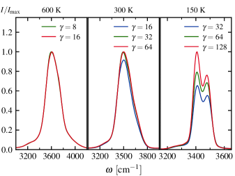
Figure 10: Simulated infrared absorption spectra in the OH-stretch region of q-TIP4P/F water at $600$, $300$, and 150 K, calculated with the AQCMD algorithm of Sec. IV at different levels of adiabatic separation $\gamma$. In all cases the position of the absorption maximum remains largely unchanged with increasing $\gamma$, and only the intensity is noticeably affected. The spectrum at 300 K demonstrates that convergence of the intensity may be quite abrupt, and similar behaviour is anticipated at $150~{}$\mathrm{K}$$.

The convergence with respect to $\gamma$ for ice at 150 K was tested using a larger simulation box of 96 molecules (in order to give zero net dipole momenthayward ). The highest value tested was $\gamma=128$, which was sufficient to converge the positions of all the bands in the spectrum, but not the relative intensity of the bend and stretch bands (see Fig. 10). A value of $\gamma=64$ was sufficient to converge the dipole-derivative TAF at $t=0$. This, together with the abrupt nature of convergence at $300~{}$\mathrm{K}$$, suggests that the $\gamma=128$ spectrum is close to convergence at 150 K.

Appendix D LMon-4 and TRPMD+GLE spectra for water

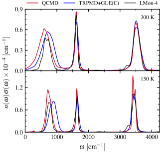
Figure 11: Infrared absorption spectra from the same simulations as Fig. 8, showing also the libration and bend regions.

For completeness we compare in Fig. 11 the full IR spectra calculated using the QCMD, TRPMD+GLE(C) and LMon-4 methods (the stretch regions of the spectra are also plotted in Fig. 8 and discussed in Sec. V.2.3). As mentioned in Sec. V.2.3, LMon-4 and TRPMD+GLE(C) are known to provide poor descriptions of the libration band.

References

- (1) J.L. Skinner, B.M. Auer, and Y.-S. Lin, Advances in Chemical Physics (Wiley-Blackwell, 2009), pp. 59–103.
- (2) S.M. Gruenbaum, C.J. Tainter, L. Shi, Y. Ni, and J.L. Skinner, J. Chem. Theory Comput. 9, 3109 (2013).
- (3) H. Liu, Y. Wang, and J.M. Bowman, J. Am. Chem. Soc. 136, 5888 (2014).
- (4) H. Liu, Y. Wang, and J.M. Bowman, J. Phys. Chem. B 118, 14124 (2014).
- (5) W.H. Miller, J. Phys. Chem. A 105, 2942 (2001).
- (6) J. Liu and W.H. Miller, J. Chem. Phys. 131, 074113 (2009).
- (7) J. Liu, Int. J. Quantum Chem. 115, 657 (2015).
- (8) Q. Shi and E. Geva, J. Phys. Chem. A 107, 9059 (2003).
- (9) J.A. Poulsen, G. Nyman and P.J. Rossky, J. Chem. Phys. 119, 12179 (2003).
- (10) J. Liu, W.H. Miller, G.S. Fanourgakis, S.S. Xantheas, S. Imoto, and S. Saito, J. Chem. Phys. 135, 244503 (2011).
- (11) X. Liu and J. Liu, Mol. Phys. 116, 755 (2018).
- (12) E. Mangaud, S. Huppert, T. Plé, P. Depondt, S. Bonella, and F. Finocchi, J. Chem. Theory Comput. 15, 2863 (2019).
- (13) M. Basire, D. Borgis, and R. Vuilleumier, Phys. Chem. Chem. Phys. 15, 12591 (2013).
- (14) J. Vaníček, W.H. Miller, J.F. Castillo, and F.J. Aoiz, J. Chem. Phys. 123, 054108 (2005).
- (15) J. Vaníček and W.H. Miller, J. Chem. Phys. 127, 114309 (2007).
- (16) J.O. Richardson, J. Chem. Phys. 144, 114106 (2016).
- (17) J.O. Richardson, J. Chem. Phys. 148, 200901 (2018).
- (18) J. Cao and G.A. Voth, J. Chem. Phys. 100, 5106 (1994).
- (19) I.R. Craig and D.E. Manolopoulos, J. Chem. Phys. 121, 3368 (2004).
- (20) I.R. Craig and D.E. Manolopoulos, J. Chem. Phys. 122, 084106 (2005).
- (21) T.F. Miller and D.E. Manolopoulos, J. Chem. Phys. 123, 154504 (2005).
- (22) S. Habershon, D.E. Manolopoulos, T.E. Markland, and T.F. Miller III, Annu. Rev. Phys. Chem. 64, 387 (2013).
- (23) M. Rossi, M. Ceriotti, and D.E. Manolopoulos, J. Chem. Phys. 140, 234116 (2014).
- (24) J.O. Richardson and S.C. Althorpe, J. Chem. Phys. 131, 214106 (2009).
- (25) T.J.H. Hele and S.C. Althorpe, J. Chem. Phys. 138, 084108 (2013).
- (26) N. Boekelheide, R. Salomón-Ferrer, and T.F. Miller III, Proc. Natl. Acad. Sci. 108, 16159 (2011).
- (27) J.S. Kretchmer and T.F. Miller III, J. Chem. Phys. 138, 134109 (2013).
- (28) G.R. Medders and F. Paesani, J. Chem. Theory Comput. 11, 1145 (2015).
- (29) S.K. Reddy, D.R. Moberg, S.C. Straight, and F. Paesani, J. Chem. Phys. 147, 244504 (2017).
- (30) D. Chandler and P.G. Wolynes, J. Chem. Phys. 74, 4078 (1981).
- (31) M. Parrinello and A. Rahman, J. Chem. Phys. 80, 860 (1984).
- (32) D.M. Ceperley, Rev. Mod. Phys. 67, 279 (1995).
- (33) S.D. Ivanov, A. Witt, M. Shiga, and D. Marx, J. Chem. Phys. 132, 031101 (2010).
- (34) A. Witt, S.D. Ivanov, M. Shiga, H. Forbert, and D. Marx, J. Chem. Phys. 130, 194510 (2009).
- (35) M. Rossi, H. Liu, F. Paesani, J. Bowman, and M. Ceriotti, J. Chem. Phys. 141, 181101 (2014).
- (36) M. Rossi, V. Kapil, and M. Ceriotti, J. Chem. Phys. 148, 102301 (2018).
- (37) T.J.H. Hele, M.J. Willatt, A. Muolo, and S.C. Althorpe, J. Chem. Phys. 142, 134103 (2015).
- (38) G. Trenins and S.C. Althorpe, J. Chem. Phys. 149, 014102 (2018).
- (39) K.K.G. Smith, J.A. Poulsen, G. Nyman, and P.J. Rossky, J. Chem. Phys. 142, 244112 (2015).
- (40) M.J. Willatt, M. Ceriotti, and S.C. Althorpe, J. Chem. Phys. 148, 102336 (2018).
- (41) T.J.H. Hele, M.J. Willatt, A. Muolo, and S.C. Althorpe, J. Chem. Phys. 142, 191101 (2015).
- (42) W.H. Miller, N.C. Handy, and J.E. Adams, J. Chem. Phys. 72, 99 (1980).
- (43) B.T. Sutcliffe and J. Tennyson, Mol. Phys. 58, 1053 (1986).
- (44) C.F. Jackels, Z. Gu, and D.G. Truhlar, J. Chem. Phys. 102, 3188 (1995).
- (45) D. Marx and M.H. Müser, J. Phys.: Condens. Matter 11, R117 (1999).
- (46) H. Kleinert, Path Integrals in Quantum Mechanics, Statistics, Polymer Physics, and Financial Markets (World Scientific, 2009), pp. 697–751.
- (47) J. Cao and G.A. Voth, J. Chem. Phys. 101, 6168 (1994).
- (48) T.D. Hone and G.A. Voth, J. Chem. Phys. 121, 6412 (2004).
- (49) T.D. Hone, P.J. Rossky, and G.A. Voth, J. Chem. Phys. 124, 154103 (2006).
- (50) J.-P. Ryckaert, G. Ciccotti, and H.J.C. Berendsen, J. Comput. Phys. 23, 327 (1977).
- (51) H.C. Andersen, J. Comput. Phys. 52, 24 (1983).
- (52) M. Tuckerman, Statistical Mechanics: Theory and Molecular Simulation (OUP, Oxford, 2010).
- (53) C. Eckart, Phys. Rev. 47, 552 (1935).
- (54) E.B. Wilson, J.C. Decius, and P.C. Cross, Molecular Vibrations: The Theory of Infrared and Raman Vibrational Spectra (Dover Publications, 1980), pp. 11–13.
- (55) A prefactor of has been cancelled out.
- (56) No thermally accessible instanton cross-over radius has been found in the -constrained ring-polymer distributions.
- (57) The spring force is equal to minus the gradient of , where is the Jacobian defined in Eq. (B).
- (58) H. Partridge and D.W. Schwenke, J. Chem. Phys. 106, 4618 (1997).
- (59) D.W. Schwenke and H. Partridge, J. Chem. Phys. 113, 6592 (2000).
- (60) W.H. Press, S.A. Teukolsky, B.P. Flannery, and W.T. Vetterling, Numerical Recipes in FORTRAN 77 (Cambridge University Press, 1992).
- (61) J. Tennyson, M.A. Kostin, P. Barletta, G.J. Harris, O.L. Polyansky, J. Ramanlal, and N.F. Zobov, Comput. Phys. Commun. 163, 85 (2004).
- (62) F. Paesani and G.A. Voth, J. Chem. Phys. 129, 194113 (2008).
- (63) R.D. Coalson, J. Chem. Phys. 85, 926 (1986).
- (64) B. Leimkuhler and C. Matthews, Proc. R. Soc. A 472, 20160138 (2016).
- (65) M. Ceriotti, M. Parrinello, T.E. Markland, and D.E. Manolopoulos, J. Chem. Phys. 133, 124104 (2010).
- (66) S. Habershon, G.S. Fanourgakis, and D.E. Manolopoulos, J. Chem. Phys. 129, 074501 (2008).
- (67) See the supplementary material for ref. trpmd2, .
- (68) S. Habershon, T.E. Markland, and D.E. Manolopoulos, J. Chem. Phys. 131, 024501 (2009).
- (69) F. Jørgensen, Int. J. Quantum Chem. 14, 55 (1978).
- (70) K.N. Kudin and A.Y. Dymarsky, J. Chem. Phys. 122, 224105 (2005).
- (71) In the absence of an external torque, the Eckart-like condition minimises the spread of the ring-polymer distribution around the orientational angles.
- (72) To evaluate exactly we would need to express it in terms of cartesian bead coordinates by inverting the nine conditions imposed by Eqs. (25) and (33).
- (73) D. Frenkel and B. Smit, Understanding Molecular Simulation: From Algorithms to Applications (Elsevier Science, 2001).
- (74) M.P. Allen and D.J. Tildesley, Computer Simulation of Liquids (Oxford Science Publications, 1989).
- (75) T. Schneider and E. Stoll, Phys. Rev. B 17, 1302 (1978).
- (76) G. Bussi and M. Parrinello, Comput. Phys. Commun. 179, 26 (2008).
- (77) V. Kapil et al., Comput. Phys. Commun. 236, 214 (2019).
- (78) Y. Wang and J.M. Bowman, J. Chem. Phys. 134, 154510 (2011).
- (79) Y. Wang and J.M. Bowman, J. Chem. Phys. 136, 144113 (2012).
- (80) M. Rossi, personal communication (2019).
- (81) K.M. Hunter, F.A. Shakib, and F. Paesani, J. Phys. Chem. B 122, 10754 (2018).
- (82) Polarisable water dipole-moment surfaces are highly non-linear functions of position, but despite this, classical, CMD and TRPMD simulations of the peak intensities show good overall agreement with experiment. This implies that the main function of the non-linearity is to provide an inhomogenous distribution of local dipole moments, each of which fluctuates almost linearly (although a small Matsubara contribution cannot be ruled out). We thus expect similar behaviour (although with better line shapes and positions) for any future QCMD calculations using these surfaces.
- (83) J.A. Hayward and J.R. Reimers, J. Chem. Phys. 106, 1518 (1997).