Solving the Bethe-Salpeter Equation in Minkowski Space for a Fermion-Scalar system

Abstract

The ladder Bethe-Salpeter Equation of a bound $(1/2)^{+}$ system, composed by a fermion and a scalar boson, is solved in Minkowski space, for the first time. The formal tools are the same already successfully adopted for two-scalar and two-fermion systems, namely the Nakanishi integral representation of the Bethe-Salpeter amplitude and the light-front projection of the fulfilled equation. Numerical results are presented and discussed for two interaction kernels: i) a massive scalar exchange and ii) a massive vector exchange, illustrating both the correlation between binding energies and the interaction coupling constants, as well as the valence content of the interacting state, through the valence probabilities and the light-front momentum distributions. In the case of the scalar exchange, an interesting side effect, to be ascribed to the repulsion generated by the small components of the Dirac spinor, is pointed out, while for the vector exchange the manifestation of the helicity conservation opens new interesting questions to be addressed within a fully non-perturbative framework, as well as the onset of a scale-invariant regime.

I Introduction

Within the relativistic quantum field theory, the intrinsically non-perturbative nature of a bound system can be suitably treated by an integral equation, like the homogeneous Bethe-Salpeter equation (BSE) Salpeter and Bethe (1951). As it is well-known, the path-integral approach on the Euclidean lattice is the main tool for addressing the non perturbative regime. However, efforts to get actual solutions of the BSE in Minkowski space, where the physical processes take place, are highly desirable. In order to carry out in its full glory the program of constructing a continuous approach, able to yield a phenomenological description of the dynamics inside bound systems in Minkowski space, one has to consider fundamental ingredients in the BSE, that make us immediately understand the big challenge to be faced. Schematically, main ingredients in the BSE are in order; i) the dressed propagators of the constituents and quanta, ii) the fully dressed interaction kernel, constructed from the two-particle-irreducible diagrams. This means that in order to get a refined description of the dynamics inside a composite relativistic system one cannot limit to consider the BSE, but one has to widen the framework including the Dyson-Schwinger equations (DSEs) for the self-energies and, in principle, an infinite tower of DSEs that consistently determine the above ingredients. In view of establishing a workable set of integral equations for studying the adopted Lagrangian, a coherent truncation scheme of the aforementioned infinite DSE tower, but able to preserve the symmetries dictated by the investigated interaction, is a prerequisite, (see, e.g., Ref. Binosi et al. (2016), for a recent study of the issue, and references quoted therein). Since more than two decades, the Euclidean space has been the elective one where successful efforts have been carried out for developing the above sketched framework, based on both BSE and DSEs for the self-energies, with a well-controlled set of approximations, like the so-called rainbow-ladder approximation. Starting from the seminal review Roberts and Williams (1994), where the general framework was illustrated by presenting the formalism for both QED and QCD together with some first results, very soon the applications to hadron physics became more and more sophisticated. As a matter of fact, the main features of the non-Abelian gauge theory of the strong interaction, like confinement and dynamical symmetry breaking, were addressed in an extended way (see, e.g., Refs. Alkofer and von Smekal (2001); Maris and Roberts (2003)), providing constant improvements in the description of hadron observables, like mesonic and baryonic spectra as well as electromagnetic properties in the space-like region, directly addressable in the Euclidean space (see, e.g., Refs. Tandy (2003); Fischer (2006); Bashir et al. (2012); Eichmann et al. (2016)). The interested reader can straightforwardly realize the huge amount of improvements reached in both formalism and obtained results by the continuous approach in the Euclidean space (a recent introduction to the numerical methods can be found in Ref. Sanchis-Alepuz and Williams (2018)) and appreciate the attempts to extend the BSE+DSE framework to the Minkowski space, for investigating light-like and time-like quantities (considering also a due cross-check for the space-like ones)

On the Minkowski side, though the necessity of elaborating a similar framework is universally recognized (see, e.g., Refs. Roberts and Williams (1994); Eichmann et al. (2016), just to mention reviews well-distant in time) one has a rather elementary stage in the development, basically i) one does not take into accout self-energies and vertex corrections and ii) considers interaction kernels mainly in ladder approximation (at most with cross-ladder contributions). Nonetheless non trivial results can be achieved, as briefly illustrated below, particularly with regard to the evaluation of both longitudinal and transverse light-front momentum distributions, not directly addressable within a Euclidean framework without introducing ad hoc paths to be carefully treated, like, e.g., analytic continuations (with all the well-known caveats about the singularities in the complex plane) or re-summation of infinite Mellin moments. In order to bring the Minkowskian approach to the level of sophistication of the Euclidean one, we need to build a systematic study of systems with different degrees of freedom, so that we can gain the physical intuition useful for guiding the next step, i.e. the application of the approach to the gap equation (as some groups are elaborating, e.g., Refs. Sauli (2003); Mezrag (2019)). Indeed, one could even devise an intermediate step, helpful for phenomenological applications, by adopting the proposal contained in Ref. Mello et al. (2017), where pion observables were evaluated by using a Bethe-Salpeter (BS) amplitude in Minkowski space (notice that in the quoted work an Ansatz was considered), together with a dressed quark propagator extracted from lattice data.

In this work, we illustrate how to solve the homogeneous BSE, in ladder approximation without vertex and self-energy corrections, for a fermion-scalar system with positive parity, i.e. with quantum numbers $J^{\pi}=(1/2)^{+}$, directly in Minkowski space. Indeed, the achievements illustrated in what follows are part of a more general investigation of the BSE in Minkowski space, carried out within an approach based on (i) the so-called Nakanishi integral representation (NIR) of the BS amplitude (see, e.g., Ref. Nakanishi (1971) for the general presentation of the framework applied to the n-leg transition amplitudes) and (ii) the light-front (LF) projection of the BSE, i.e. its restriction to a vanishing relative LF time (an introduction to this technique and its application to the BSE is given in Frederico et al. (2012)). This approach, together with the analogous one developed by Carbonell and Karmanov (see, e.g., Karmanov and Carbonell (2006a); Carbonell and Karmanov (2006, 2010)), has already achieved relevant outcomes, addressing: i) two-scalar systems both in bound states and at the zero-energy limit Frederico et al. (2012, 2014, 2015); Gutierrez et al. (2016); the two-fermion bound state in a $0^{+}$ channel de Paula et al. (2016, 2017). To summarize the results of the previous studies and of the present one, we can state that such an approach is able to yield actual solutions of the BSE, directly in Minkowski space. Therefore one can be confident to reach a consistent (with the set of assumptions discussed in what follows) and reliable description of the inner dynamics of relativistic systems, such that it becomes feasible the evaluation of relevant quantities, like the valence component of the system. Within the BSE approach, one can obtain a non-perturbative description of the dynamics inside the system, in a space endowed with a $SO(3,1)$ symmetry, since an integral equation is able to sum up all the infinite contributions generated by the interaction kernel, though truncated at a given order in the coupling constant Noteworthy, there are efforts to go beyond the ladder approximation by including the cross-ladder diagrams as shown in Refs. Carbonell and Karmanov (2006); Karmanov and Carbonell (2006b); Gigante et al. (2017), as well as to explore the formal inversion of the NIR, as in Ref. Carbonell et al. (2017), for eventually exploiting a Wick-rotated formulation of the BSE. It should be pointed out that the inversion is an ill-posed problem that needs non trivial elaborations to be accomplished. For instance, in Ref. Chang et al. (2013) (for a recent Bayesian approach to the inversion, see Ref. Gao et al. (2017)), the challenge of the inversion has been well illustrated, showing how the pion parton distribution function could be evaluated starting from a Euclidean framework where both the quark-antiquark BSE and the quark gap-equation are taken into account.

The target of our investigation is the $(1/2)^{+}$ bound system, composed by a fermion and a scalar. As a prototype of such a system one could consider a mock nucleon composed by a quark and a point-like scalar diquark (see, e.g., Ref. Alkofer and von Smekal (2001); Eichmann et al. (2016) and references quoted therein for a general introduction to the description of a baryon in terms of confined quark and extended diquarks, with the last feature needed for implementing the correct statistics), or even a more exotic bound system as the ghost-quark one investigated, e.g. in Ref. Alkofer and Alkofer (2011). In order to broad our study, we allowed the constituents to interact through two possible interaction Lagrangians: i) ${\cal L}=\lambda^{s}_{F}\bar{\psi}\psi\chi+\lambda^{s}_{S}\phi^{*}\phi\chi$ and ii) ${\cal L}=\lambda^{v}_{F}\bar{\psi}/\!\!\!V\psi-i\lambda^{v}_{S}\phi^{*}\overleftrightarrow{\partial}_{\mu}\phi V^{\mu}$, where only the coupling constant $\lambda^{s}_{S}$ has a mass dimension, while the other three couplings are dimensionless. The fields $\psi$ and $\phi$ describe the fermionic and bosonic constituents, respectively, while $\chi$ and $V^{\mu}$ are the fields of the exchanged scalar and vector bosons. It is worth noticing that in the mock nucleon (representing only a first step in the avenue for developing a Minkowskian approach for investigating an actual nucleon), the only explicit vector boson exchange is between the quark and the point-like diquark, while in the modern approach the nucleon is bound by a quark exchange and the gluon exchange is buried in the interaction kernel Buck et al. (1992); Alkofer and von Smekal (2001); Eichmann et al. (2016). Hence, at the present stage, one can obtain the description of a massive quark-diquark system only in the region dominated by the one-gluon exchange as it is discussed in Sect. IV, while for the massless ghost-quark bound system it is necessary at least to dress the interaction in order to break the scale invariance that the bare vertex brings about.

The BS amplitude for the system we are addressing is

$$\Phi^{\pi}(k,p,J_{z})=\int{d^{4}x}~{}e^{ik\cdot x}~{}\langle 0|T\{\psi(x/2)~{}\phi(-x/2)\}|p;J,J_{z},\pi\rangle~{}~{},$$ (1)

where $p=p_{F}+p_{S}$ is the total four-momentum of the system, with $p^{2}=M^{2}$ ($M$ is the mass of the bound system), while the relative four-momentum is given by $k=\eta_{1}p_{F}-\eta_{2}p_{S}$ (N.B. $\eta_{1}+\eta_{2}=1$). We use $\eta_{i}=1/2$, obtaining

$$p_{F(S)}={p\over 2}\pm k~{}~{}.$$

The conjugate BS amplitude is obtained analyzing the residue of the 4-leg Green’s function at the bound pole (assuming for the sake of simplicity, to be only one), and it reads

$$\bar{\Phi}^{\pi}(k,p,J_{z})=\int{d^{4}x}~{}e^{-ik\cdot x}~{}\langle\pi,J_{z},J;p|T\{\bar{\psi}(x/2)~{}\phi^{*}(-x/2)\}|0\rangle$$ (2)

As it is well-known, the BS amplitude for a bound state fulfills the following homogeneous BSE, where we discard, at the present stage of our investigation, both self-energy and vertex corrections,

$$\Phi^{\pi}(k,p,J_{z})=G_{0}(p/2-k)S(p/2+k)\int{d^{4}k^{\prime}\over(2\pi)^{4}}~{}i{\cal K}^{Ld}(k,k^{\prime},p)~{}\Phi^{\pi}(k^{\prime},p,J_{z})~{},$$

(3)

with the relevant propagators given by

$$G_{0}(q)~{}=i~{}{1\over(q^{2}-m^{2}_{S}+i\epsilon)}~{}~{},\quad\quad S(q)~{}=i~{}{/\!\!\!q+m_{F}\over(q^{2}-m^{2}_{F}+i\epsilon)}$$ (4)

In our calculations in ladder approximation, we adopt the following momentum-dependent kernels for scalar and vector exchanges

$$i{\cal K}^{Ld}_{s}(k,k^{\prime},p)=-i~{}\lambda^{s}_{S}\lambda^{s}_{F}~{}{1\over(k-k^{\prime})^{2}-\mu^{2}+i\epsilon}~{}~{},$$ (5)

and

$$i{\cal K}^{Ld}_{v}(k,k^{\prime},p)=-i~{}\lambda^{v}_{S}\lambda^{v}_{F}~{}{(/\!\!\!p-/\!\!\!k-/\!\!\!k^{\prime})\over(k-k^{\prime})^{2}-\mu^{2}+i\epsilon}$$ (6)

with $\mu$ the mass of the exchanged boson.

Actually the interaction kernel for the scalar case does not depend upon the total momentum of the system, while in the vector-exchange case it does, since the bosonic current is the sum of the initial and final momenta. Moreover, it should be pointed out that the propagator of the exchanged-vector is given in the Feynman gauge.

Aim of the present work is to study Eq. (3) by using both the NIR of the BS amplitude and the LF-projection technique in order to obtain an eigen-equation formally equivalent to the initial BSE. After that, one can proceed to numerically solve the eigenvalue problem and calculate several quantities and functions through which it is possible to investigate more deeply the inner dynamics. In particular, in correspondence to the two aforementioned interactions, one can calculate, e.g., i) the relevant correlation between the binding energy of the system and the coupling constant, ii) the probability of the valence component, as well as iii) the longitudinal and transverse LF-momentum distributions. The peculiar features of the LF distributions allow one to shed some light on intriguing effects, that noteworthy manifest themselves after carrying out non-trivial dynamical calculations. The proposed physical interpretations, in terms of small components of the constituent fermion and its polarization, seem to herald new interesting analysis, particularly for the vector interaction, where the onset of a scale-invariant regime could appear beside a clear evidence of the effect of the helicity conservation, for the larger values of the binding energy considered in the present work.

The paper is organized as follows. In Sect. II the general formalism of NIR is introduced and the eigenvalue problem formally equivalent to the ladder BSE is worked out; in Sect. III the probability and the LF distributions are defined; in Sect. IV the numerical results are thoroughly presented and discussed. Finally, in Sect. V, conclusions are drawn and some interesting perspectives shortly illustrated.

II BSE and the Nakanishi integral representation

In order to solve Eq. (3), one proceeds through three main steps (for the two-fermion system see, e.g., Carbonell and Karmanov (2010); de Paula et al. (2016, 2017)), namely: i) writing down the most general expression of the BS amplitude $\Phi^{\pi}(k,p,J_{z})$ for the system under scrutiny, ii) introducing the NIR and iii) projecting Eq. (3) onto the null-plane $x^{+}=x^{0}+x^{3}=0$. This series of operations allows to get the desired solutions in Minkowski space.

The fermion-scalar BS amplitude has a Dirac index, and after exploiting Lorentz invariance, parity and the Dirac equation for the whole system, it can be written as follows

$$\Phi^{\pi}(k,p,J_{z})=\Bigl{[}O_{1}(k)~{}\phi_{1}(k,p)+O_{2}(k)~{}\phi_{2}(k,p)\Bigl{]}~{}U(p,J_{z})~{}~{},$$ (7)

where $\phi_{i}$ are unknown scalar functions that depend upon the available momenta and are determined by solving the BSE. The operators $O_{i}$ act on the spinor $U$ (with normalization $\bar{U}~{}U=1$) and one has

$$O_{1}(k)=\mathbb{I}~{}~{},\quad\quad O_{2}(k)={/\!\!\!k\over M}~{}~{},\quad\quad(/\!\!\!p-M)~{}U(p,J_{z})=0~{}~{}.$$ (8)

In order to get the equations fulfilled by the scalar functions $\phi_{i}(k,p)$, one can multiply both sides of Eq. (3) by $O_{i}(k)$, and evaluate the following traces, ${\cal N}_{ij}$ and ${\cal T}_{ij}$,

$${\cal N}_{ij}=Tr\left[O_{i}(k)~{}O_{j}(k)~{}{(/\!\!\!p+M)\over 2M}\right]$$

$${\cal T}^{s(v)}_{ij}(k,k^{\prime},p)=Tr\left[O_{i}(k)~{}(/\!\!\!p_{F}+m_{F})~{}\Gamma^{s(v)}~{}O_{j}(k^{\prime})~{}{(/\!\!\!p+M)\over 2M}\right]~{}~{},$$ (9)

where $\Gamma^{s}=1$ and $\Gamma^{v}=/\!\!\!p-/\!\!\!k-/\!\!\!k^{\prime}$. Through this formal elaboration, one is able to transform Eq. (3) into an equivalent coupled system of integral equations for the scalar functions $\phi^{s(v)}_{i}(k,p)$, viz

$$\phi^{s(v)}_{i}(k,p)={i\over(p/2-k)^{2}-m^{2}_{S}+i\epsilon}~{}{i\over(p/2+k)^{2}-m^{2}_{F}+i\epsilon}\int{d^{4}k^{\prime}\over(2\pi)^{4}}$$

$$\times~{}{(-i{\lambda^{s(v)}_{S}}\lambda^{s(v)}_{F})\over(k-k^{\prime})^{2}-\mu^{2}+i\epsilon}~{}\sum_{j=1,2}{\cal C}^{s(v)}_{ij}(k,k^{\prime},p)~{}\phi^{s(v)}_{j}(k^{\prime},p)~{}~{},$$ (10)

with

$${\cal C}^{s(v)}_{1j}(k,k^{\prime},p)=~{}{M^{2}\over 2}~{}{k^{2}{\cal T}^{s(v)}_{1j}-(k\cdot p){\cal T}^{s(v)}_{2j}\over k^{2}M^{2}-(p\cdot k)^{2}}$$

$${\cal C}^{s(v)}_{2j}(k,k^{\prime},p)=-{M^{2}\over 2}~{}{(k\cdot p){\cal T}^{s(v)}_{1j}-M^{2}{\cal T}^{s(v)}_{2j}\over k^{2}M^{2}-(p\cdot k)^{2}}~{}~{}.$$ (11)

For the sake of simplicity, in what follows we drop out the notation ${s(v)}$, indicating the type of interacting kernel one is considering, but it will be restored when needed. The actual expressions of ${\cal C}_{ij}(k,k^{\prime},p)$, for the scalar and vector exchanges are given in Appendices A and B, respectively.

As in the case of a system composed by two scalars Karmanov and Carbonell (2006a); Carbonell and Karmanov (2006); Frederico et al. (2014, 2015); Gutierrez et al. (2016) or by two fermions Carbonell and Karmanov (2010); de Paula et al. (2016, 2017)), one can introduce the NIR for each scalar function $\phi_{i}(k,p)$

$$\phi_{i}(k,p)=\int_{-\infty}^{\infty}d\gamma^{\prime}\int_{-1}^{1}dz^{\prime}\frac{g_{i}(\gamma^{\prime},z^{\prime};\kappa^{2})}{[{k}^{2}+z^{\prime}p\cdot k-\kappa^{2}-\gamma^{\prime}+i\epsilon]^{3}}~{}~{},$$ (12)

where the real functions $g_{i}(\gamma,z;\kappa^{2})$ are called Nakanishi weight functions (NWFs), that depend upon real variables, and

$$\kappa^{2}=\bar{m}^{2}-{M^{2}\over 4}~{}~{},$$ (13)

with $\bar{m}=(m_{F}+m_{S})/2$.

In order to complete this first part, we mention that in Appendix C the actual expression of the BS-amplitude normalization, both in terms of the scalar functions $\phi_{i}$ and the NWFs $g_{i}$, is presented.

II.1 Determining the Nakanishi weight functions

The appealing motivation for using the expressions in Eq. (12) as trial functions for solving the homogeneous BSE, is the possibility to make apparent the analytic structure of the BS amplitude, as dictated by the analysis performed by Nakanishi in a perturbative framework Nakanishi (1971). It is important to stress that the validity of this procedure is numerically demonstrated a posteriori, i.e. at the end of the formal elaboration we are going to carry out, without further assumptions beyond the one shown in Eq. (12). As a matter of fact, one eventually gets a generalized eigenvalue problem, and if one finds solutions, acceptable from the physical point of view (i.e. real eigenvalues), then one can state that the expression in Eq. (12) is flexible enough to obtain actual solutions of the equivalent BSE.

The last main step is the so-called LF projection of the BSE, since it is based on the introduction of LF coordinates $k^{\pm}=k^{0}\pm k_{z}$. As it is well-known, a practical advantage in adopting these variables is the possibility to split multifold poles in the variable $k^{0}$ in poles for the variables $k^{+}$ and $k^{-}$. This simple observation (that can be rephrased in a different formal environment given in Refs. Karmanov and Carbonell (2006a); Carbonell and Karmanov (2010), where the explicitly-covariant LF framework is adopted) becomes crucial for obtaining a substantial simplification of the analytical integrations one has to face with in what follows (for the sake of comparison see the two-scalar case presented in Ref. Kusaka et al. (1997)). The LF projection of the BSE amounts to integrate both sides of Eq. (10) on $k^{-}$ (see, e.g., Frederico et al. (2012) and references therein quoted). Notice that such a formal step means to restrict the relative LF-time to a vanishing value. The main advantage of applying the LF projection (or the equivalent approach in Refs. Karmanov and Carbonell (2006a); Carbonell and Karmanov (2010)) is given by the formally exact reduction of the 4D BSE into an equivalent coupled system for determining the NWFs $g_{i}(\gamma,z;\kappa^{2})$. However, one should bear in mind that the LF projection of the BS amplitude produces another important outcome, since it allows one to obtain the valence component of the interacting state, so that a probabilistic content can be usefully established in the BS approach.

The LF projection of the scalar functions $\phi_{i}$, Eq. (12), reads (see Frederico et al. (2014); de Paula et al. (2016, 2017) for details)

$$\int_{-\infty}^{\infty}\frac{d{k}^{-}}{2\pi}\int_{-\infty}^{\infty}d\gamma^{\prime}\int_{-1}^{1}dz^{\prime}\frac{g_{i}(\gamma^{\prime},z^{\prime};\kappa^{2})}{[{k}^{2}+z^{\prime}p\cdot k-\kappa^{2}-\gamma^{\prime}+i\epsilon]^{3}}=$$

$$={-i\over M}\int_{-\infty}^{\infty}d\gamma^{\prime}~{}\frac{g_{i}(\gamma^{\prime},z;\kappa^{2})}{\left[\gamma^{\prime}+\gamma+(1-z^{2})\kappa^{2}+z^{2}\bar{m}^{2}-i\epsilon\right]^{2}}~{}~{},$$ (14)

where $\gamma=|{\bf k}_{\perp}|^{2}$, $z=-2k^{+}/M$.

Let us apply the LF projection also to the rhs of Eq. (10), in strict analogy to the fermionic case de Paula et al. (2016, 2017), but with a substantial simplification in the treatment of the LF singularities, generated by the behavior along the arc for large $k^{-}$ in the complex plane (see also Ref. Yan (1973) for the first discussion of those singularities and the method to fix them). In particular, the mentioned LF singularities do not affect the fermion-scalar case, and one can write the following coupled system

$$\int_{\gamma_{min}}^{\infty}d\gamma^{\prime}\frac{g_{i}(\gamma^{\prime},z;\kappa^{2})}{\left[\gamma^{\prime}+\gamma+(1-z^{2})\kappa^{2}+z^{2}\bar{m}^{2}-i\epsilon\right]^{2}}={\lambda_{F}~{}\lambda_{S}\over 2(4\pi)^{2}}~{}{1\over D_{0}(\gamma,z)}~{}$$

$$\times~{}\int_{0}^{1}dv~{}v^{2}\int_{\gamma_{min}}^{\infty}d\gamma^{\prime}\int_{-1}^{1}dz^{\prime}~{}\sum_{j=1,2}~{}~{}g_{j}(\gamma^{\prime},z^{\prime};\kappa^{2})$$

$$\times\left[{(1+z)^{2}~{}B_{ij}(k^{-}_{u})\theta(z^{\prime}-z)\over D_{u}^{2}(z^{\prime},z,m^{2}_{S})}+{(1-z)^{2}~{}B_{ij}(k^{-}_{d})\theta(z-z^{\prime})\over D_{d}^{2}(z^{\prime},z,m^{2}_{F})}\right]~{}~{},$$ (15)

where

$$D_{0}(\gamma,z)=\gamma+(1-z^{2})\kappa^{2}+(\Delta-z\bar{m})^{2}~{}~{},$$ (16)

and $\gamma_{min}=-2z\bar{m}|\Delta|+\Delta^{2}$, with $\Delta=(m_{S}-m_{F})/2$. The lower extremum $\gamma_{min}$ is determined in order to avoid a free propagation in the BS amplitude of a bound state, i.e. by requiring the absence of cuts. The denominator $D_{u}$ (for $z^{\prime}>z$) is

$$D_{u}(z^{\prime},z,m^{2}_{S})=v(1-v)~{}(z^{\prime}-z)~{}\left[\gamma-(1-z^{2}){M^{2}\over 4}+m^{2}_{S}\right]$$

$$+(1+z)~{}\left[v(1-v)\left(\gamma+z^{2}{M^{2}\over 4}\right)+v(\gamma^{\prime}+\kappa^{2})+v^{2}z^{\prime 2}{M^{2}\over 4}+(1-v)\mu^{2}\right]~{}~{},$$ (17)

Notice that

$$\lim_{z^{\prime}\to z}~{}{D_{u}(z^{\prime},z,m^{2}_{S})\over(1+z)}=v(1-v)~{}\gamma+vz^{2}{M^{2}\over 4}+v(\gamma^{\prime}+\kappa^{2})+(1-v)\mu^{2}~{}~{},$$ (18)

and therefore, in this limiting case, the factor $(1+z)^{2}$ in the numerator is exactly canceled.

When $z>z^{\prime}$, the denominator is $D_{d}(z^{\prime},z,m^{2}_{F})=D_{u}(-z^{\prime},-z,m^{2}_{F})$, and the same limit for $z^{\prime}\to z$ is obtained for $D_{d}(z^{\prime},z,m^{2}_{F})/(1-z)$.

Moreover, in Eq.(15) one has

$$\begin{array}[]{l l l}B_{11}(k^{-}_{u(d)})=c^{(0)}_{11}+c^{(1)}_{11}k^{-}_{u(d)}~{},&{}{}{}{}{}&B_{12}(k^{-}_{u(d)})=c^{(0)}_{12}+c^{(1)}_{12}k^{-}_{u(d)}\\ B_{21}(k^{-}_{u(d)})=c^{(0)}_{21}~{},&{}{}{}{}{}&B_{22}(k^{-}_{u(d)})=c^{(0)}_{22}+c^{(1)}_{22}k^{-}_{u(d)}\end{array}~{}~{},$$ (21)

where the coefficients $c^{(i)}_{jk}$ for scalar and vector exchanges are given in Appendices A and B, respectively, and

$$k^{-}_{u}=\frac{M}{2}-{2~{}(\gamma+m^{2}_{S})\over M(1+z)}={~{}p^{-}\over 2}-p^{-}_{S,on}~{},\quad k^{-}_{d}=-\frac{M}{2}+{2~{}(\gamma+m^{2}_{F})\over M(1-z)}=-{~{}p^{-}\over 2}+p^{-}_{F,on}~{}~{}.$$ (22)

It is very important to remind that $k^{-}_{u}$ corresponds to have the scalar constituent on its mass-shell, and hence the fermion is highly virtual, while for $k^{-}_{d}$ the opposite happens.

The key point is to recognize Eq. (15) as a generalized eigenvalue problem. The eigenvectors are the pair of NWFs $\{g_{1},g_{2}\}$, and the corresponding eigenvalues are the product of the coupling constants $\lambda_{F}\lambda_{S}$ (or quantities proportional to them, see below). Once the mass $M$ of the system is assigned, one can proceed through standard numerical methods (cf Sect. IV). Indeed, the coupled system depends non linearly upon the mass of the system, that can be written as

$$M=2\bar{m}-B$$

where $B$ is the binding energy. The acceptable values of $B/\bar{m}$ fall in the range $[0,2]$ (see Refs. Baym (1960); Şavkli et al. (1999) for a discussion of the critical behavior of a $\phi^{3}$ model).

III Probability and LF-momentum distributions of the valence component

As it is well-known, the BS amplitude does not have a probabilistic interpretation, while exploiting a LF Fock expansion of the interacting state Brodsky et al. (1998) one can retrieve a probabilistic framework, so important and helpful for our physical intuition. To accomplish this, one exploits the LF wave functions, i.e. the amplitudes of the Fock expansion of the interacting states (in the present case $~{}|(1/2)^{+}\rangle~{}$). They are invariant under LF boosts, and fulfill the following normalization constraint (see Appendix D for notations and details)

$$2(2\pi)^{3}\sum_{n}\int\big{[}d\xi_{i}\big{]}\left[d^{2}\mbox{\boldmath{$\kappa$}}_{i\perp}\right]\,\left|\psi^{J\pi}_{n}(\{\xi_{i}\}_{n};\{{\mbox{\boldmath{$\kappa$}}}_{i\perp}\}_{n};\{\sigma_{i}\}_{n_{F}};J_{z})\right|^{2}=1~{}~{},$$ (23)

where (i) $\psi^{J\pi}_{n}$ are the LF wave functions, i.e. the amplitudes of the Fock state with $n$ particles (fermions and bosons) and (ii) $\{\xi_{i},{\mbox{\boldmath{$\kappa$}}}_{i\perp}\}$ are the LF-boost invariant kinematical variables of the i-th particles Brodsky et al. (1998). The LF wave function with the lowest number of constituents, i.e. one fermion and one scalar, is the valence wave function. From Eq. (23), it follows that the probability to find the valence component in the interacting state with $J=1/2$ and given $J_{z}$ is (see also Appendix D)

$$P_{val}={1\over(2\pi)^{3}}~{}\sum_{\sigma_{1}}\int_{0}^{1}{d\xi\over 2~{}\xi(1-\xi)}\int d^{2}{\mbox{\boldmath{$\kappa$}}}_{\perp}~{}\left|\psi^{J\pi}_{n=2}(\xi;{\mbox{\boldmath{$\kappa$}}}_{\perp};\sigma_{1};J_{z})\right|^{2}~{}~{}.$$ (24)

After establishing the definitions within the Fock-expansion framework, it is compelling to find the relation between the valence component and the BS amplitude, given its relevance in the application to hadron physics. In view of this, it is useful to recall that the intrinsic description of the system contained in the valence component is the one living onto the $x^{+}=0$ hyperplane, as one can straightforwardly realize performing the 4D Fourier transform of the valence component, that has no dependence on $k^{-}$ (conjugated to the LF-time $x^{+}$). Moreover, one of the external legs of the BS amplitude is a fermion, and one should avoid any possible kinematical singularity related to the instantaneous propagation (i.e. with $x^{+}=0$), since the valence component does not have such an analytic behavior. This amounts to cut in the fermionic propagator the term $\gamma^{+}/(2k^{+})$. The announced relation is (see Appendix D for more details)

$$\psi^{J\pi}_{n=2}(\xi;{\mbox{\boldmath{$\kappa$}}}_{\perp};\sigma_{1};J_{z})={(1-\xi)}~{}\sqrt{m_{F}\over 2}\int{dk^{-}\over 2\pi}~{}\bar{u}_{\alpha}(\tilde{q}_{1},\sigma_{1})\gamma^{+}_{\alpha\beta}\Phi^{\pi}_{\beta}(k,p;J_{z})$$ (25)

with $\tilde{q}_{1}\equiv\{\xi p^{+},{\mbox{\boldmath{$\kappa$}}}_{\perp}\}$ and ${\bf p}_{\perp}=0$.

By introducing in the rhs of Eq. (25) the expression of the BS amplitude (7), one finds the following components of the valence wave function in terms of the scalar functions $\phi_{i}(k,p)$, (cf Eq. (14))

$$\tilde{\phi}_{i}(\xi,\gamma;\kappa^{2})=iM\int_{-\infty}^{\infty}{dk^{-}\over 2\pi}\phi_{i}(k,p)=\int_{-\infty}^{\infty}d\gamma^{\prime}~{}\frac{g_{i}(\gamma^{\prime},z;\kappa^{2})}{\left[\gamma^{\prime}+\gamma+(1-z^{2})\kappa^{2}+z^{2}\bar{m}^{2}-i\epsilon\right]^{2}}~{}~{},$$ (26)

where

$$\xi={q^{+}_{1}\over p^{+}}={k^{+}\over p^{+}}+{1\over 2}={1-z\over 2}$$ (27)

Hence, for the LF valence wave function one writes

$$\psi^{J\pi}_{n=2}(q^{+}_{1}/p^{+};{\bf q}_{1\perp};\sigma_{1};J_{z})=-i~{}(1-\xi)~{}\sqrt{\xi\over 2M}$$

$$\times~{}\left\{\delta_{\sigma_{1},J_{z}}\left[\tilde{\phi}_{1}(\xi,\gamma;\kappa^{2})-{z\over 2}~{}\tilde{\phi}_{2}(\xi,\gamma;\kappa^{2})\right]-\delta_{-\sigma_{1},J_{z}}~{}2J_{z}~{}{k_{x}+i2J_{z}k_{y}\over M}~{}\tilde{\phi}_{2}(\xi,\gamma;\kappa^{2})\right\}~{}~{}.$$ (28)

Notably, in Eq. (28) the two contributions stemming from the configurations with the spins of the constituent and the system aligned or anti-aligned are well identified. Finally combining Eqs. (24) and (28), one writes

$$P_{val}=P^{A}_{val}+P^{noA}_{val}$$ (29)

where the probabilities of the aligned and anti-aligned configurations are given by

$$P^{A}_{val}={1\over 32M\pi^{2}}~{}\int_{0}^{1}{d\xi~{}(1-\xi)}\int_{0}^{\infty}d{\gamma}~{}\left[\tilde{\phi}_{1}(\xi,\gamma;\kappa^{2})-{z\over 2}\tilde{\phi}_{2}(\xi,\gamma;\kappa^{2})\right]^{2}$$

$$P^{noA}_{val}={1\over 32M\pi^{2}}~{}\int_{0}^{1}{d\xi~{}(1-\xi)}\int_{0}^{\infty}d{\gamma}~{}{\gamma\over M^{2}}~{}\tilde{\phi}^{2}_{2}(\xi,\gamma;\kappa^{2})~{}~{}.$$ (30)

Another set of quantities quite relevant for understanding the dynamics in the valence component, and consequently interesting from the experimental point of view, is given by the LF valence distributions, that describe i) the probability distribution to find a constituent with a given longitudinal fraction $\xi$ and ii) the probability distribution to find a constituent with transverse momentum $\gamma=|{\bf k}_{\perp}|^{2}$. They are defined for the fermionic constituent as follows

$$\phi^{F}(\xi)={1\over 32M\pi^{2}}~{}~{}(1-\xi)\int_{0}^{\infty}d{\gamma}~{}\left[\left(\tilde{\phi}_{1}(\xi,\gamma;\kappa^{2})-{z\over 2}\tilde{\phi}_{2}(\xi,\gamma;\kappa^{2})\right)^{2}+{\gamma\over M^{2}}~{}\tilde{\phi}^{2}_{2}(\xi,\gamma;\kappa^{2})\right]$$ (31)

$${\cal P}^{F}(\gamma)={1\over 32M\pi^{2}}~{}\int_{0}^{1}{d\xi~{}(1-\xi)}~{}\left[\left(\tilde{\phi}_{1}(\xi,\gamma;\kappa^{2})-{z\over 2}\tilde{\phi}_{2}(\xi,\gamma;\kappa^{2})\right)^{2}+{\gamma\over M^{2}}~{}\tilde{\phi}^{2}_{2}(\xi,\gamma;\kappa^{2})\right]$$ (32)

and are normalized to $P_{val}$. One can easily recognize the two contributions: the aligned and the anti-aligned ones.

IV Numerical Results

The numerical method for solving the coupled system in Eq. (15) strictly follows the one already adopted for the two-fermion case de Paula et al. (2016, 2017). Basically, one expands the NWFs on an orthonormal basis given by the Cartesian product of Laguerre polynomials and Gegenbauer ones, in order to take care of the dependence upon $\gamma$ and $z$, respectively. Unfortunately, in the case of the fermion-boson system one cannot exploit the symmetry under the exchange of the two constituents (i.e. $z\to-z$) for constraining the symmetry of the BS amplitude, and in turn of the NWFs (particularly the odd or even dependence upon $z$). Hence, the adopted orthonormal basis contains both symmetric and antisymmetric Gegenbauer polynomials. The expansion of the $g_{i}$ reads

$$g_{i}(\gamma,z;\kappa^{2})=\sum_{m=0}^{\infty}\sum_{n=0}^{\infty}A_{mn}^{i}(\kappa^{2})~{}G^{\nu_{i}}_{m}(z)\,\mathcal{J}_{n}(\gamma)~{},$$ (33)

where i) $A_{mn}^{i}$ are suitable coefficients to be determined by solving the generalized eigen-problem given by the coupled-system (15), ii) $G^{\nu_{i}}_{m}(z)$, are related to the Gegenbauer polynomials $C_{m}^{\nu_{i}}(z)$, while iii) $\mathcal{J}_{n}(\gamma)$ are given in terms of the Laguerre polynomials $L_{n}(a\gamma)$. In particular, one has

$$G_{n}^{\nu}(z)=(1-z^{2})^{q}~{}~{}\Gamma(\nu)\sqrt{\frac{n!(n+\nu)}{2^{1-2\nu}\,\pi\,\Gamma(n+2\nu)}}~{}C_{n}^{\nu}(z)~{},$$

$$\mathcal{J}_{n}(\gamma)=\sqrt{a}\,L_{n}(a\gamma)e^{-a\gamma/2}~{}.$$ (34)

where $q=(2\nu-1)/4$ has been taken equal to $1$ for $g_{1}$ and $3$ for $g_{2}$, respectively. The parameter $a$ governs the fall-off of the NWFs for large $\gamma$ and it turns out that when $M$ becomes smaller and smaller, decreasing its value is helpful from the numerical point of view. Indeed, for smaller values of the mass, the system is more compact, and therefore the kinetic energy increases, emphasizing the relevance of the tail in $\gamma$ of the NWFs. In order to speed up the convergence of the integration on $\gamma$, this variable has been rescaled by a factor $a_{0}$, i.e. $\gamma\to\gamma/a_{0}$. In the actual calculation, $a_{0}$ has been chosen equal to $12$, while $a=6$.

Two general observations are in order: i) after introducing the above expansion and the proper projection, the lhs of (15) reduces to a symmetric real matrix applied to a vector containing the coefficients of the expansion, while the rhs contains a non symmetric matrix, ii) the eigenvalues can be real or complex conjugated. In conclusion, one symbolically writes

$$L(M)~{}{\mbox{\boldmath{$v$}}}=\alpha~{}R(M)~{}{\mbox{\boldmath{$v$}}}$$ (35)

where the non linear dependence upon the mass of the system, $M$, is present in both sides. The search of the eigenvalues, i.e. the coupling constant compatible with the assigned mass $M$, proceeds by looking for the lowest real eigenvalue, which corresponds to the shallowest well able to support a bound system with mass $M$, if one exploits a physical intuition based on a simple, non-relativistic instance. The smallest eigenvalue is obtained by using first a low number of basis functions in the expansion in Eq. (33), and then checking the stability of the result by increasing the basis. To determine the eigenvectors, i.e. the coefficients in the expansion (33), requests more care. For getting more stable results, following Ref. Karmanov and Carbonell (2006a), a small quantity $\epsilon=10^{-8}$ has been added to the diagonal elements of the lhs matrix, and furthermore both sides of Eq. (15) have been multiplied by a factor $(1-z^{2})^{p}$, that helps to enforce the constraint at the extrema of the variable $z$. The used values for the exponent $p$ is $1$ for the scalar exchange and $2$ for the vector one. Finally, the following numerical results correspond to the maximal values for $m$ and $n$ in Eq. (33) $N_{Lag}=N_{Geg}=56$.

IV.1 Scalar interaction

In order to get rid of the dimensional dependence on the mass, the coupling constant for the scalar exchange is defined as follows

$$\alpha^{S}={\lambda^{s}_{F}~{}\lambda^{s}_{S}\over 8\pi m_{S}}~{}~{}.$$ (36)

Notice that the factor $8\pi$ is twice the familiar $4\pi$, in order to match the non-relativistic reduction of the Born term in the fermion-scalar scattering, properly taking into account the different relativistic normalization of fermionic and bosonic states. Table 1 shows the coupling constants for the case of a scalar exchange and equal-mass constituents, i.e. $m_{F}=m_{S}$. In particular, the presented results correspond to binding energies in unit mass $B/\bar{m}\in[0.1,1]$ and two values of the exchanged-boson mass $\mu/\bar{m}=0.15,~{}0.50$. For the sake of comparison, in Table 1, it is also shown the analogous set of results evaluated after Wick-rotating the relative variables $k_{0}$ and $k^{\prime}_{0}$ in Eq. (10), namely without inserting LF coordinates, but keeping the standard ones and changing both $k_{0}\to ik_{0}$ and $k^{\prime}_{0}\to ik^{\prime}_{0}$. It is worth noticing that the values of the dimensionless coupling constant for the scalar exchange are larger than the ones shown in Table 3, corresponding to the vector exchange. Such a difference can be seen also for the two-fermion case de Paula et al. (2017), and it can be ascribed to the repulsion generated by the small component of the fermion spinor when a scalar vertex is involved. As a matter of fact, the scalar interaction meets a difficulty to bind a system, when it becomes more and more compact (i.e. $B$ increases). In order to identify the source of the repulsion that opposes the binding, one should analyze the low $M$ behavior of the coefficients $B_{ij}(k^{-}_{u(d)})$ given in Eq. (21). After inserting the coefficients shown in Eq. (40) and $k^{-}_{u(d)}$ from Eq. (22), one gets that only $B_{12}(k^{-}_{u})$ is always negative for $m_{S}>M/2$ and it becomes larger and larger (in modulus) for $M\to 0$ (strong coupling limit), viz

$$B_{12}(k^{-}_{u})=-\frac{z^{\prime}v}{2}\left(\frac{M}{2}+{m}_{F}\right)-{\left(1-v\right)\over M(1+z)}~{}\left[2\gamma+(1-z)\left(m^{2}_{S}-{M^{2}\over 4}\right)+z^{2}{M^{2}\over 2}\right]$$ (37)

The numerical checks, obtained after omitting this negative term, show an almost $40\%$ reduction of the coupling $\alpha^{S}$, for $\mu/\bar{m}=0.5$ and $B/\bar{m}=1$, with $P_{val}=0.82$, and the calculations can be even extended to $B/\bar{m}>1$ without any large increase of the coupling constant, as well as a smoother growing of $P_{val}$. The physical source of the repulsion can be heuristically understood once we recall that the fermion-scalar vertex, when initial and final fermions are on-mass shell, contains the scalar density $\bar{u}~{}u$, and the Dirac matrix $\gamma^{0}$ generates a minus sign in front of the contribution produced by the small components. Hence a repulsion is produced. Moreover, one should expect that the repulsive effect of the small components of the fermion spinor is driven by the kinetic energy, since the scalar density is written in terms of the large Dirac component, $f$, and the small one, $g$, as follows: $\rho_{s}=\bar{u}u\sim|f({\bf k})|^{2}-|g({\bf k})|^{2}\sim\rho_{v}-2|{\bf k}~{}f({\bf k})|^{2}/(E+m)^{2}$, with the vector density given by $\rho_{v}=u^{\dagger}u\sim|f({\bf k})|^{2}+|g({\bf k})|^{2}$.

Table 1: Scalar coupling $\alpha^{S}$, Eq. (36), for $m_{F}=m_{S}$ and $\mu/\bar{m}=0.15,~{}0.50$ (with $\bar{m}=(m_{S}+m_{F})/2$). First column: the binding energy in unit mass of $\bar{m}$, i.e. $B/\bar{m}$. Second and fourth columns: coupling constants $\alpha^{S}_{M}$, obtained by solving the BSE (3) in Minkowski space through Eq. (15). Third and fifth columns: Wick-rotated results, $\alpha^{S}_{WR}$ (see text).

$B/\bar{m}$	$\alpha^{S}_{M}(0.15)$	$\alpha^{S}_{WR}(0.15)$	$\alpha^{S}_{M}(0.50)$	$\alpha^{S}_{WR}(0.50)$
0.10	1.506	1.506	2.656	2.656
0.20	2.297	2.297	3.624	3.624
0.30	3.047	3.047	4.535	4.535
0.40	3.796	3.796	5.451	5.451
0.50	4.568	4.568	6.404	6.404
0.80	7.239	7.239	9.879	9.879
1.00	9.778	9.778	13.738	13.738

For illustrative purpose, in Fig. 1, the NWFs for the scalar exchange with $\mu/\bar{m}=0.15$ and equal-mass constituents, are presented as a function of i) $\gamma$ and fixed $z=0$ and ii) $z$ and fixed $\gamma=0$, respectively. Interestingly, the difference between $g_{1}$ and $g_{2}$ increases for large binding energies. Indeed, such an effect could be related to the weight in front of $\phi_{2}$, i.e. the factor $/\!\!\!k/M$ (cf Eq. (7)). As a matter of fact, for increasing $B/\bar{m}$ the average size of the system decreases and large values of the kinetic energy (related to the relative momentum $k$) become more and more likely, and in order to avoid a blowing contribution from the second term in Eq. (7), the amplitude $\phi_{2}$ should decrease. The same happens for larger values of $\mu/\bar{m}$, since the system becomes more compact, given the shrinking of the range of the interaction. It is worth mentioning that the NWFs can have wild oscillatory behaviors, that fade out in a smooth pattern of the LF distributions, discussed in what follows, given the filtering role played by the integral kernel in Eq. (26). Such an effect is well-known in the analysis of signals where the generalized Stieltjes transforms are commonly adopted (see, e.g. Ref. Link et al. (1991)).

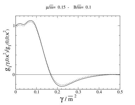
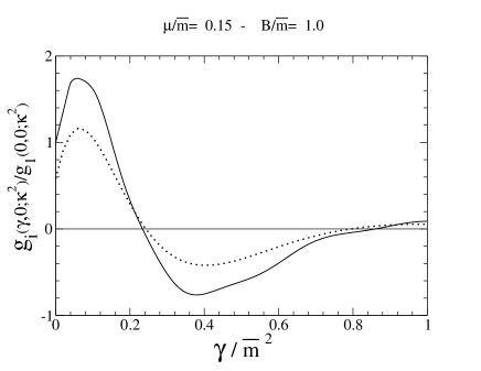
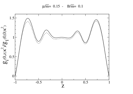
Figure 1: The Nakanishi weight functions $g_{i}$ for an equal-mass $(1/2)^{+}$ system, and the interaction mediated by a scalar boson with $\mu/\bar{m}=0.15$. Left side: the calculations with $B/\bar{m}=0.1$. Right side: calculations with $B/\bar{m}=1$. Solid line : $g_{1}$. Dotted line: $g_{2}$. Upper panels: $g_{i}$ vs $\gamma$, and $z=0$. Lower panels: $g_{i}$ vs $z$, and $\gamma=0$. Notice that the normalization factor is the same for both NWFs, namely $g_{1}(0,0;\kappa^{2})$.

The relevance of the valence component in the Fock expansion of the interacting state is illustrated in Table 2, where the valence probabilities, defined in Eq. (24), are shown together with the two contributions from the possible configurations of the spin of the system and the spin of the constituent, namely i) aligned or ii) anti-aligned. In the second case, one must have a component of the orbital angular momentum ${L}=1$ in order to get a third component of the total momentum equal to $J_{z}=\pm 1/2$. The valence probabilities start to behave in an unexpected way when the binding increases. This seems to indicate that the repulsion we mentioned above damps the coupling of the valence state with the higher Fock-components, and consequently the valence probability increases. Indeed, the large kinetic energy needed to allow a compact system (the size is related to the inverse of the binding energy) is more efficiently shared on a two-constituent Fock state than on multi-particle ones.

Further insights can be gained from the analysis the LF-momentum distributions, presented in what follows.

Table 2: Valence probabilities (see Eq. (24)), for the scalar exchange with $m_{F}=m_{S}$ and $\mu/\bar{m}=0.15,~{}0.50$. The two contributions, $P^{noA}_{val}$ and $P^{A}_{val}$, corresponding to the configurations where the spin of the constituent is anti-aligned or aligned to the spin of the system, are also shown. First column: the binding energy in unit mass of $\bar{m}$.

$\mu/\bar{m}=0.15$

$\mu/\bar{m}=0.50$

$B/\bar{m}$	$P_{val}$	$P^{noA}_{val}$	$P^{A}_{val}$	$P_{val}$	$P^{noA}_{val}$	$P^{A}_{val}$
0.10	0.81	0.02	0.79	0.88	0.03	0.85
0.20	0.77	0.03	0.74	0.85	0.05	0.80
0.30	0.76	0.05	0.71	0.84	0.07	0.77
0.40	0.75	0.06	0.69	0.83	0.09	0.74
0.50	0.76	0.07	0.69	0.83	0.11	0.72
0.80	0.81	0.13	0.68	0.88	0.18	0.70
1.00	0.90	0.19	0.71	0.98	0.25	0.73

In Figs. 2 and 3, the longitudinal and transverse LF distributions (cf Eqs. (31) and (32)), are shown for the fermion in the valence component, with $\mu/\bar{m}=0.15,~{}0.50$, and three-values of the binding energy $B/\bar{m}=0.1,~{}0.5,~{}1$. The longitudinal distribution shows a peak around $\xi=0.5$ for $B/\bar{m}=0.1$, that broadens and sizably reduces its height (slightly shifting towards lower values of $\xi$), when the binding energy and/or the mass of the exchanged boson increase. The behavior substantially follows the increasing pattern of the anti-aligned probability (that involves the orbital $L=1$ component). This observation suggests that the fermion, to be considered almost massless for large kinetic energy, tends toward a positive helicity. Indeed, the increasing of the tail at $\xi\geq 0.8$ (for $B/\bar{m}>1$ a sizable bump appears) is given by the aligned configuration, and the large values of $\xi$ mean a Cartesian 3-momentum aligned along the positive $z$-axis. Differently, the anti-aligned configuration dominates the probability at small values of $\xi$ (i.e. a Cartesian 3-momentum along the negative direction of the $z$-axis), and again one recovers a preferred positive helicity. Notice that also the transverse distribution follows a pattern correlated to the growing of the average kinetic energy, as it happens for bigger values of $B/\bar{m}$ and/or the exchanged-boson mass.

As a final remark, we mention that the values of the average $<\xi>$ follows a slightly decreasing pattern from $0.5$ for $B/\bar{m}=0.1$ to $0.41$ at $B/\bar{m}=1$, almost irrespective of the value of $\mu/\bar{m}$, while for $<\gamma/\bar{m}^{2}>$ one goes from $0.09$ to $0.47$ with $\mu/\bar{m}=0.15$, and from $0.15$ to $0.64$ with $\mu/\bar{m}=0.50$.

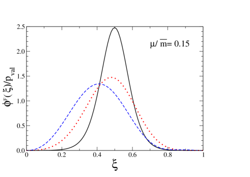
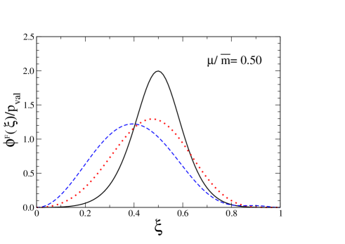
Figure 2: (Color online). Longitudinal LF distributions for a fermion in the valence component for $\mu/\bar{m}=0.15$ (left panel) and for $\mu/\bar{m}=0.50$ (right panel), in the case of a scalar exchange. Solid line: $B/\bar{m}=0.1$. Dotted red line: $B/\bar{m}=0.5$. Dashed blue line: $B/\bar{m}=1.0$.

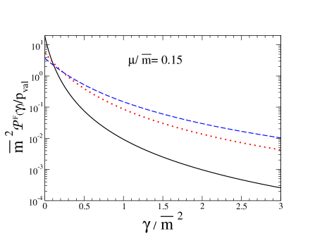
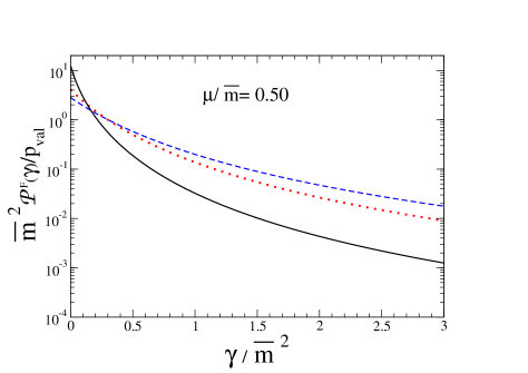
Figure 3: (Color online). Transverse LF distributions for a fermion in the valence component for $\mu/\bar{m}=0.15$ (left panel) and for $\mu/\bar{m}=0.50$ (right panel), in the case of a scalar exchange. Solid line: $B/\bar{m}=0.1$. Dotted red line: $B/\bar{m}=0.5$. Dashed blue line: $B/\bar{m}=1.0$.

IV.2 Vector interaction

For the vector exchange case, the coupling constant is defined as

$$\alpha^{V}={\lambda^{v}_{F}~{}\lambda^{v}_{S}\over 8\pi}$$ (38)

and it does not contain any mass in the denominator, given the dimensionless nature of the vertex constants in the interaction Lagrangian. Being dimensionless the vertex constants, the BSEs both in Euclidean and in Minkowski spaces, as well as the system of integral equations for the NWF, have the property to be invariant under a scale transformation in the ultraviolet region. Such a symmetry imposes a maximum value for the coupling constant, beyond which the invariance is broken. One encounters a similar situation in the fermion-fermion bound state problem in the ladder approximation both in Euclidean Dorkin et al. (2008) and in Minkowski space Carbonell and Karmanov (2010). Here, we adopt a conservative point of view and present calculations for moderate bindings, leaving the detailed study of the scale invariance breaking, that should establish at larger bindings, for a future work Alvarenga Nogueira et al. (2019). Our results in Minkowski space, shown in Table 3 up to $B/\bar{m}=0.5$, nicely agree with the Wick-rotated calculations, analogously to what happens for the scalar-exchange case.

Table 3: Vector coupling $\alpha^{V}$, Eq. (38), for $m_{F}=m_{S}$ and $\mu/\bar{m}=0,~{}0.15,~{}0.50$. First column: the binding energy in unit mass of $\bar{m}$, i.e. $B/\bar{m}$. Second, fourth and sixth column: coupling constants $\alpha^{V}_{M}$, obtained by solving the BSE (3) in Minkowski space through Eq. (15). Third, fifth and seventh column: Wick-rotated results, $\alpha^{V}_{WR}$, with a numerical uncertainty for $B/\bar{m}=0.5$ due to some instabilities in the Gaussian quadrature adopted.

$B/\bar{m}$	$\alpha^{V}_{M}(0)$	$\alpha^{V}_{WR}(0)$	$\alpha^{V}_{M}(0.15)$	$\alpha^{V}_{WR}(0.15)$	$\alpha^{V}_{M}(0.50)$	$\alpha^{V}_{WR}(0.50)$
0.10	0.513	0.513	0.608	0.609	0.849	0.854
0.20	0.758	0.761	0.823	0.823	1.009	1.015
0.30	0.936	0.938	0.979	0.978	1.127	1.129
0.40	1.074	1.074	1.107	1.097	1.225	1.216
0.50	1.189	1.18 $\pm$ .03	1.214	1.19 $\pm$ .03	1.311	1.28 $\pm$ .04

In Table 4, the valence probabilities are shown for the vector exchange. In the range of $B/\bar{m}$ we have investigated, as dictated by the onset of a scale-invariant regime, they smoothly decrease.

Table 4: The same as in Table 2, but for the vector exchange.

$\mu/\bar{m}=0.0$

$\mu/\bar{m}=0.15$

$\mu/\bar{m}=0.50$

$B/\bar{m}$	$P_{val}$	$P^{noA}_{val}$	$P^{A}_{val}$	$P_{val}$	$P^{noA}_{val}$	$P^{A}_{val}$	$P_{val}$	$P^{noA}_{val}$	$P^{A}_{val}$
0.10	0.69	0.01	0.68	0.73	0.02	0.71	0.75	0.04	0.71
0.20	0.62	0.02	0.60	0.64	0.03	0.61	0.66	0.05	0.61
0.30	0.57	0.03	0.54	0.58	0.04	0.54	0.60	0.06	0.54
0.40	0.53	0.04	0.49	0.54	0.05	0.49	0.55	0.07	0.48
0.50	0.50	0.05	0.45	0.50	0.05	0.45	0.52	0.07	0.45

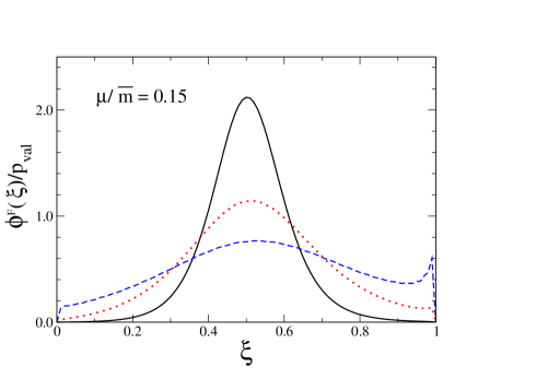
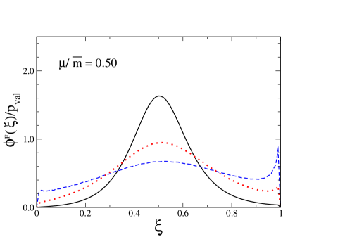
Figure 4: (Color online). Longitudinal LF distributions for a fermion in the valence component for $\mu/\bar{m}=0.15$ (left panel) and for $\mu/\bar{m}=0.50$ (right panel), in the case of a vector exchange. Solid line: $B/\bar{m}=0.1$. Dotted red line: $B/\bar{m}=0.3$. Dashed blue line: $B/\bar{m}=0.5$.

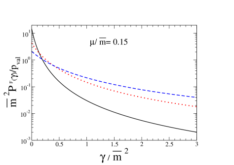
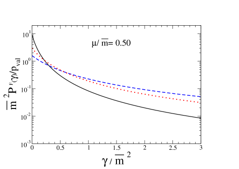
Figure 5: (Color online). Transverse LF distributions for a fermion in the valence component for $\mu/\bar{m}=0.15$ (left panel) and for $\mu/\bar{m}=0.50$ (right panel), in the case of a vector exchange. Solid line: $B/\bar{m}=0.1$. Dotted red line: $B/\bar{m}=0.3$. Dashed blue line: $B/\bar{m}=0.5$.

Figures 4 and 5 illustrate the peculiar pattern of the longitudinal and transverse LF distributions, respectively. As already noticed for the scalar case, for increasing $B/\bar{m}$ the size of the system decreases and the average kinetic energy of the constituents becomes bigger and bigger. This favors the orbital $L=1$ component of the valence wave function, and produces an increasing of the non-aligned configuration, mainly close at $\xi=0$. As shown in Fig. 4, the longitudinal distribution acquires a particular shape for increasing $B/\bar{m}$, emphasizing what we have started to see in the scalar-exchange case. The calculations show that the dominant contribution for $\xi\to 1$ is given by the aligned configuration and for $\xi\to 0$ by the anti-aligned one. After recalling that for $\xi\to 1$ and $\xi\to 0$ the fermion has a maximal Cartesian component along its spin, one can say that the fermion in both cases has a positive helicity. Such a result can be interpreted in the light of the conservation of the angular momentum within the LF quantum-field theory, or equivalently of the helicity conservation for the vector interaction (see Ref. Chiu and Brodsky (2017) for a recent work elucidating this issue). In conclusion, it is gratifying that the outcome of a non-trivial dynamical calculation is in full agreement with the physical expectation from a conservation law.

The transverse distributions show the familiar fall-off that becomes less and less pronounced for increasing $B/\bar{m}$, following what we have already learned about the increasing of the kinetic energy.

For the sake of completeness, we quote also the average values of $<\xi>$ and $<\gamma/\bar{m}^{2}>$ . In particular, $<\xi>$ follows a slightly increasing pattern from $0.51$ for $B/\bar{m}=0.1$ to $0.55$ at $B/\bar{m}=1.0$ (almost irrespective of for $\mu/\bar{m}$), and $<\gamma/\bar{m}^{2}>$ ranges from $0.17$ to $5.9$ (for $\mu/\bar{m}=0.50$, the corresponding values are $0.44$ and $6.8$).

It is worth noticing that the onset of the helicity conservation should be investigated in more detail, in particular by exploring the impact of a non pointlike interaction vertex, i.e. different from the one assumed in the present work.

In Fig. 6, the LF distributions for a fermion-scalar system with different masses of the constituents is presented. In order to start a first survey of a mock nucleon we have chosen a mass ratio $m_{S}/m_{F}=2$ and a binding energy $B/\bar{m}=~{}0.1$ (e.g., $M_{N}/\bar{m}=1.9$). Also in this case we adopted $\mu/\bar{m}=0.15$ and $\mu/\bar{m}=0.50$. The corresponding values for the coupling constants are $\alpha^{V}=0.648$ and $\alpha^{V}=0.898$, respectively, while for the valence probabilities we have found $P_{val}=0.75$ and $P_{val}=0.77$, that means a quite large valence component. It is very rewarding and of phenomenological interest to recognize the signature of the scale invariance in the behavior of the tail of the transverse-momentum distributions. As a matter of fact, extending the calculations for $\gamma/\bar{m}^{2}>40$ the fall-off can be described by $C_{1}/\gamma^{2.26}$ for $\mu/\bar{m}=0.15$, and $C_{2}/\gamma^{2.43}$ for $\mu/\bar{m}=0.50$, in agreement with the values predicted by the scale invariance analysis in Ref. Alvarenga Nogueira et al. (2019). Indeed, even if the model is elementary, since both self-energy and vertex corrections are absent and only the one-vector exchange is taken into account (notice that such an interaction should govern the tail of the momentum distributions, also in more refined approaches) this kind of analysis could suggest the proper framework, where a study of the scale invariance could be started, analyzing the departures from the evaluations we are providing.

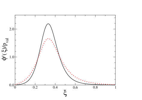
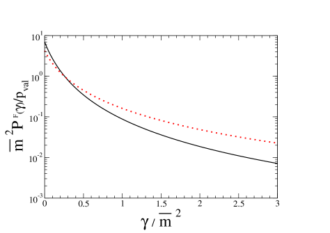
Figure 6: (Color online). Light-front distributions for a fermion in the valence component of the state $(1/2)^{+}$, with a mass ratio $m_{S}/m_{F}=2$ and a binding $B/\bar{m}=~{}0.1$. Left panel: longitudinal distribution. Right panel transverse-momentum distribution. Solid line: $\mu/\bar{m}=0.15$. Dotted line: $\mu/\bar{m}=0.50$ .

V Conclusions

The present study of the ladder Bethe-Salpeter equation describing an interacting system, composed by a fermion and a scalar, has been performed by adopting an approach based on the Nakanishi integral representation of the BS amplitude and the light-front framework. In particular, two interactions have been applied: i) the scalar interaction and ii) the vector one (in Feynman gauge). This model, though simple, already allows one to start a dynamical investigation of intrinsic features, like i) in the scalar exchange case, the repulsive effects that could pose a limitation to the use of the ladder kernel in the strong-coupling regime, and ii) in the vector case, the effects of the helicity conservation, as well as of the scale-invariant regime and beyond, that will be investigated elsewhere Alvarenga Nogueira et al. (2019).

Moreover, one has to emphasize the absence of the exchange symmetry, working for the two-scalar and two-fermion systems.

The coupling constants for assigned masses of the interacting system have been obtained as an outcome of an eigenvalue problem, formally deduced from the initial BSE, and compared with the corresponding results where the BSE is solved after introducing a Wick rotation. The agreement, as in the case of two-scalar Karmanov and Carbonell (2006a); Frederico et al. (2014) and two-fermion systems Carbonell and Karmanov (2010); de Paula et al. (2016, 2017), is very good, and adds more and more confidence in the adopted approach.

To conclude, a benefit of any technique able to solve the BSE in Minkowski space is the direct access to the LF distributions, that have been shown in Figs. 2, 3, 4, 5 and 6. For the equal-mass case, the very peculiar behavior of the longitudinal distributions, with a particular emphasis for the vector interaction, has allowed us to point out the nice role played by the two possible configurations of the constituent and system spins. In the case of the vector interaction, when states of large momentum are more and more populated for increasing values of the coupling constant, the fermion longitudinal distribution sizably cumulates close to $\xi\to 0$ and $\xi\to 1$, yielding a clear evidence of the action of the helicity conservation law. Furthermore, it should be interesting to notice that the relative weight of the orbital $L=1$ (anti-aligned configuration) with respect to the $L=0$ one (aligned configuration) is around 10% for both interactions, at $B/\bar{m}=0.5$, with an increasing behavior for increasing binding energies. The unequal-mass case with a vector-exchange interaction, i.e. a mock nucleon composed by a quark and a scalar point-like diquark, with mass ratio $m_{S}/m_{F}=2$, yields the possibility to investigate the extent to which the scale invariance could affect the hadron dynamics. Indeed, our calculations, that necessarily lead to a scale-invariant behavior of the transverse-momentum distribution (cf Fig. 6), should be considered as a reference line for more refined phenomenological studies. Finally, we should point out that massless fermion-scalar systems (e.g., a ghost-quark bound state as in Ref. Alkofer and Alkofer (2011)) can be addressed only by introducing a new scale other than the masses of constituents and quanta, like the one associated to an extended interaction vertex (cf the results in Refs. de Paula et al. (2016, 2017)). This very interesting study has to be postponed to another work, where, both vertex and self-energy corrections have to be carefully treated.

Appendix A Coefficients for the scalar-boson exchange

The coefficients in Eq. (10) for the exchange of a scalar-boson are given by

$${\cal{C}}_{11}=\frac{1}{2}M+{m}_{F}$$

$${\cal{C}}_{12}={(k^{\prime}\cdot p)\over M}-{1\over M^{2}k^{2}-(k\cdot p)^{2}}\left\{{(k^{\prime}\cdot p)\over M}~{}k^{2}\left[M^{2}b+(k\cdot p)\right]\right.$$

$$\left.-(k^{\prime}\cdot k)~{}M\left[(k\cdot p)b+k^{2}\right]\right\}$$

$${\cal{C}}_{21}=M$$

$${\cal{C}}_{22}={M\over M^{2}k^{2}-(k\cdot p)^{2}}\left\{(k^{\prime}\cdot p)\left[k^{2}+b(k\cdot p)\right]-(k^{\prime}\cdot k)\left[M^{2}b+(k\cdot p)\right]\right\}$$

(39)

where

$$b=\frac{1}{2}-{m_{F}\over M}$$

The non-vanishing coefficients in Eq. (21) are given by

$$c^{(0)}_{11}={M\over 2}a$$

$$c^{(0)}_{12}=-\frac{z^{\prime}v}{2}~{}{M\over 2}a-\left(1-v\right)~{}\frac{1}{M}\left(\gamma+\frac{zM^{2}}{4}\right)~{},~{}~{}~{}~{}c^{(1)}_{12}={\left(1-v\right)\over 2}\left(1-z\right)$$

$$c^{(0)}_{21}=M$$

$$c^{(0)}_{22}=-M\frac{z^{\prime}v}{2}-\left(1-v\right)~{}Mb$$ (40)

with

$$a=1+2{m_{F}\over M}$$

Appendix B Coefficients for the vector-boson exchange

The coefficients in Eq. (10) for the exchange of a vector-boson are given by

$${\cal C}_{11}={M^{2}\over 2}a-k^{2}-(k\cdot p)-(k^{\prime}\cdot p)+{M^{2}\over 2\left[k^{2}M^{2}-(k\cdot p)^{2}\right]}$$

$$\times\left\{(2-a)\left[(k^{\prime}\cdot p)k^{2}-(k\cdot k^{\prime})(k\cdot p)\right]+2{k^{2}\over M^{2}}\left[(k^{\prime}\cdot p)(k\cdot p)-(k\cdot k^{\prime})M^{2}\right]\right\}$$

$${\cal C}_{12}=~{}-{a\over 2}k^{\prime 2}-(k^{\prime}\cdot k)+(a-1)(k^{\prime}\cdot p)+{M^{2}\over 2\left[k^{2}M^{2}-(k\cdot p)^{2}\right]}$$

$$\times~{}\left\{\left[(2-a)-2{k^{2}\over M^{2}}\right]~{}\left[(k^{\prime}\cdot p)k^{2}-(k^{\prime}\cdot k)(k\cdot p)\right]+a{k^{2}\over M^{2}}\left[(k^{\prime}\cdot p)(k\cdot p)-(k^{\prime}\cdot k)M^{2}\right]\right\}$$

$${\cal C}_{21}=(2-a){M^{2}\over 2}+M^{2}-{M^{2}\over 2\left[k^{2}M^{2}-(k\cdot p)^{2}\right]}$$

$$\times\left\{(2-a)\left[(k^{\prime}\cdot p)(k\cdot p)-(k\cdot k^{\prime})M^{2}\right]+2\left[(k^{\prime}\cdot p)k^{2}-(k\cdot k^{\prime})(k\cdot p)\right]\right\}$$

$${\cal C}_{22}=-k^{\prime 2}-(k^{\prime}\cdot k)+2(k^{\prime}\cdot p)-{M^{2}\over 2\left[k^{2}M^{2}-(k\cdot p)^{2}\right]}$$

$$\times~{}\left\{(2-a)\left[(k^{\prime}\cdot p)(k\cdot p)-(k\cdot k^{\prime})M^{2}\right]+\left[a-2{(k\cdot p)\over M^{2}}\right]~{}\left[(k^{\prime}\cdot p)k^{2}-(k\cdot k^{\prime})(k\cdot p)\right]\right\}$$

where

$$a=1+{2m_{F}\over M}$$ (42)

The coefficients in Eq. (21) are given by

$$c^{(0)}_{11}={M^{2}\over 2}\left[a+vz^{\prime}{a\over 2}+(2-v){z\over 2}\right]+(2-v)\gamma$$

$$c^{(1)}_{11}=-{M\over 2}(2-v)\left(1-z\right)$$

$$c^{(0)}_{12}={a\over 2}\left\{\gamma(1-v)(2+v)+2v(\gamma^{\prime}+\kappa^{2})+2(1-v)\mu^{2}\phantom{1\over 2}\right.$$

$$\left.+{M^{2}\over 4}(vz^{\prime}-2)[z-v(z-z^{\prime})]\right\}+\left(\gamma+z{M^{2}\over 4}\right)~{}\left(1-v-z^{\prime}{v\over 2}\right)$$

$$c^{(1)}_{12}={M\over 2}~{}\left\{a(1-v)\left[1+z+(z-z^{\prime}){v\over 2}\right]-{(1-z)}~{}\left(1-v-z^{\prime}{v\over 2}\right)\right\}$$

$$c^{(0)}_{21}={M^{2}\over 2}\left[(2-v)(2-a)+2+z^{\prime}v\right]$$

$$c^{(0)}_{22}=\gamma(1-v)(2+v)+2v(\gamma^{\prime}+\kappa^{2})+2(1-v){\mu}^{2}$$

$$+{M^{2}\over 2}\left[(1-v)\left(zz^{\prime}{v\over 2}-z+2-a\right)+z^{\prime}{v\over 2}~{}(z^{\prime}v-4+a)\right]$$

$$c^{(1)}_{22}={M\over 2}~{}(1-v)\left[v(z-z^{\prime})+2(1+z)\right]$$ (43)

Appendix C The normalization of the BS amplitude

The normalization of the BS amplitude is obtained by applying the standard expression illustrated, e.g., in Ref. Lurié et al. (1965), but adapted to the fermion-scalar case. In particular, recalling that we disregard the self-energy effects, one has the following normalization constraint

$$\int{d^{4}q\over(2\pi)^{4}}\int{d^{4}k\over(2\pi)^{4}}~{}\bar{\Phi}^{\alpha}_{p}(q,J^{\prime}_{z})~{}\left.{\partial\over\partial p_{\mu}}\Bigl{[}G^{-1}_{0}(k,p)(2\pi)^{4}\delta^{4}(q-k)-i{\cal K}(q,k,p)\Bigr{]}\right|_{p^{2}_{on}}$$

$$\times~{}\Phi^{\beta}_{p}(k,J_{z})=i2p^{\mu}~{}\delta_{J^{\prime}_{z},J_{z}}~{}\delta_{\alpha\beta}$$ (44)

where

$$G^{-1}_{0}(k,p)=-\left({p^{2}\over 4}+k^{2}-p\cdot k-m^{2}_{S}\right)~{}\left(/\!\!\!p/2+/\!\!\!k-m_{F}\right)$$ (45)

Depending upon the actual expression of the interaction kernel in ladder approximation, one has or not a contribution for the derivative of ${\cal K}$. Finally, it is worth mentioning that in ladder approximation the normalization amounts to the charge normalization.

C.1 Scalar-exchange kernel

Let us consider the scalar-exchange case. In ladder approximation the interaction kernel ${\cal K}$ does not depend upon $p$, and therefore does not contribute to the derivative in Eq. (44). By inserting the BS amplitude as given in Eq. (7), one remains in the scalar case with

$$\int{d^{4}k\over(2\pi)^{4}}~{}\bar{U}^{\alpha}(p,J^{\prime}_{z})\left[\phi_{1}(k)+{/\!\!\!k\over M}\phi_{2}(k)\right]$$

$$\times~{}\left[\left(m^{2}_{S}-{3\over 4}M^{2}-k^{2}+2p\cdot k\right)/\!\!\!p+\left(2p\cdot k-M^{2}\right)~{}(/\!\!\!k-m_{F})\right]$$

$$\times~{}\left[\phi_{1}(k)+{/\!\!\!k\over M}\phi_{2}(k)\right]U^{\beta}(p,J_{z})=i4M^{2}~{}\delta_{J^{\prime}_{z},J_{z}}~{}\delta_{\alpha\beta}$$ (46)

In the CM frame, after multiplying with the proper spinors and summing over $J^{\prime}_{z}$ and $J_{z}$, one gets

$$\int{d^{4}k\over(2\pi)^{4}}~{}{(/\!\!\!p+M)\over 2M}\left[\phi_{1}(k)+{/\!\!\!k\over M}\phi_{2}(k)\right]$$

$$\times~{}\left[\left(m^{2}_{S}-{3\over 4}M^{2}-k^{2}+2p\cdot k\right)/\!\!\!p+\left(2p\cdot k-M^{2}\right)~{}(/\!\!\!k-m_{F})\right]$$

$$\times~{}\left[\phi_{1}(k)+{/\!\!\!k\over M}\phi_{2}(k)\right]{(/\!\!\!p+M)\over 2M}=i4M^{2}~{}~{}{(/\!\!\!p+M)\over 2M}$$ (47)

where

$$\sum_{J_{z}}U(p,J_{z})\bar{U}(p,J_{z})={(/\!\!\!p+M)\over 2M}$$

and $\bar{U}(p,J_{z})U(p,J_{z})=1$.

Finally, one evaluates the traces, takes care of the NIR for $\phi_{i}$ (Eq. (12)) and performs the 4D integration by exploiting standard tricks (see, e.g., Frederico et al. (2014)), obtaining the following normalization constraint

$${M\over(8\pi)^{2}}\int_{\gamma_{min}}^{\infty}d\gamma^{\prime\prime}\int_{\gamma_{min}}^{\infty}d\gamma^{\prime}\int_{-1}^{1}dz^{\prime\prime}\int_{-1}^{1}dz^{\prime}\int_{0}^{1}dv~{}v^{2}(1-v)^{2}~{}{1\over A^{4}}~{}\Bigl{\{}N_{11}~{}g_{1}(\gamma^{\prime\prime},z^{\prime\prime};\kappa^{2})~{}g_{1}(\gamma^{\prime},z^{\prime};\kappa^{2})$$

$$+N_{12}~{}g_{1}(\gamma^{\prime\prime},z^{\prime\prime};\kappa^{2})~{}g_{2}(\gamma^{\prime},z^{\prime};\kappa^{2})+N_{22}~{}g_{2}(\gamma^{\prime\prime},z^{\prime\prime};\kappa^{2})~{}g_{2}(\gamma^{\prime},z^{\prime};\kappa^{2})\Bigr{\}}=1$$ (48)

where

$$N_{11}={\cal C}+{A\over 2M^{2}}$$

$$N_{12}=-2\left[\lambda~{}{\cal C}+{A\over 2M^{2}}\left(1+3\lambda+{m_{F}\over M}\right)\right]$$

$$N_{22}=\lambda^{2}~{}{\cal C}+{3\over 2}{A^{2}\over M^{4}}-{A\over 2M^{2}}\left[2{m_{F}\over M}-{m^{2}_{S}\over M^{2}}+{3\over 4}+{3}\lambda~{}\left(2{m_{F}\over M}+1\right)+3\lambda^{2}\right]$$ (49)

with

$${\cal C}={3\over 2}~{}\left[{m^{2}_{S}\over M^{2}}-{3\over 4}+{m_{F}\over M}-\lambda\left(1-2{m_{F}\over M}\right)+\lambda^{2}\right]$$

$$A=\kappa^{2}(1-4\lambda^{2})+v\gamma^{\prime\prime}+(1-v)\gamma^{\prime}+(2\lambda\bar{m}-\Delta)^{2}~{}~{},$$

$$\lambda=[vz^{\prime\prime}+(1-v)z^{\prime}]/2~{}~{}.$$ (50)

C.2 Vector exchange kernel

In the vector-exchange case, the interaction kernel ${\cal K}$ acquires a dependence upon the total momentum $p$, and therefore one has

$${\partial\over\partial p_{\mu}}\left[i{\cal K}(k,k^{\prime},p)\right]=-i\lambda^{v}_{S}\lambda^{v}_{F}{\gamma^{\mu}\over(k-k^{\prime})^{2}-\mu^{2}+i\epsilon}~{}~{}~{}.$$ (51)

After performing steps similar to the ones done for the scalar exchange, one obtains a contribution generated by the derivative in Eq. (51), that has to be added to the one shown in the lhs of Eq. (48). The actual form of this new contribution is

$${1\over 2M^{2}~{}(4\pi)^{3}}{\lambda^{v}_{S}\lambda^{v}_{F}\over 8\pi}\int_{\gamma_{min}}^{\infty}d\gamma^{\prime}\int_{-1}^{1}dz^{\prime}~{}\int_{\gamma_{min}}^{\infty}d\gamma\int_{-1}^{1}dz~{}~{}\int_{0}^{1}dv~{}v^{2}~{}\int_{0}^{1}d\xi{\xi^{2}~{}(1-\xi)\over\left\{D_{3}-i\epsilon\right\}^{3}}$$

$$\times~{}\left\{Mag_{1}(\gamma^{\prime},z^{\prime};\kappa^{2})g_{1}(\gamma,z;\kappa^{2})-Mbg_{1}(\gamma^{\prime},z^{\prime};\kappa^{2})g_{2}(\gamma,z;\kappa^{2})\right.$$

$$\left.+g_{2}(\gamma^{\prime},z^{\prime};\kappa^{2})g_{2}(\gamma,z;\kappa^{2})\left[z^{\prime}vb{M\over 4}+{1\over 2aM}(1-v)\left(D_{3}+b^{2}{M^{2}\over 2}\right)\right]\right\}$$ (52)

where

$$D_{3}={M^{2}\over 4}{b^{2}}+a~{}\xi(\gamma+\kappa^{2})+a~{}(1-\xi)\left[v^{2}z^{\prime 2}{M^{2}\over 4}+v(\gamma^{\prime}+\kappa^{2})+(1-v)\mu^{2}\right]$$

$$a=\xi+(1-\xi)v(1-v)~{}~{},\quad b=\xi z+(1-\xi)v(1-v)z^{\prime}$$ (53)

Appendix D The valence component

In this Appendix, the relation between the BS amplitude and the valence component of the fermion-scalar interacting state is discussed with some detail.

For illustrative purpose, we assume a scalar exchange and write the Fock expansion of the fermion-scalar interacting system as follows

$$|\tilde{p};M,JJ_{z};\pi;\rangle=2(2\pi)^{3}\sum_{n\geq 2}\sum_{n_{F}=1}^{n-1}\sum_{\{\sigma_{i}\}_{n_{F}}}~{}\int[d\xi_{i}]\int[d{\mbox{\boldmath{$\kappa$}}}_{i\perp}]$$

$$\times~{}\psi^{J\pi}_{n}(\{\xi_{i}\}_{n};\{\kappa_{i\perp}\}_{n};\{\sigma_{i}\}_{n_{F}};J_{z})~{}|\{\xi_{i}p^{+},{\mbox{\boldmath{$\kappa$}}}_{i}+\xi_{i}{\bf p}_{\perp}\}_{n};\{\sigma_{i}\}_{n_{F}}\rangle$$ (54)

where the integration symbols mean

$$\int\big{[}d\xi_{i}\big{]}\equiv\prod_{i=1}^{n}\int{d\xi_{i}\over 2~{}(2\pi)\xi_{i}}\,\delta\left(1-\sum_{j=1}^{n}\xi_{j}\right)~{}~{},$$

$$\int[d{\mbox{\boldmath{$\kappa$}}}_{i\perp}]\equiv\prod_{i=1}^{n}\int{d{\mbox{\boldmath{$\kappa$}}}_{i\perp}\over(2\pi)^{2}}~{}\delta^{2}\left(\sum_{j=1}^{n}{\mbox{\boldmath{$\kappa$}}}_{j\perp}\right)$$ (55)

In Eq. (54), the generic Fock state contains $n_{F}$ and $n_{S}$ fermionic and scalar constituents, respectively, and $n_{E}$ exchanged bosons. It is given by (recall that $n=n_{F}+n_{S}+n_{E}$)

$$|\{\tilde{q}_{i}\}_{n};\{\sigma_{i}\}_{n_{F}}\rangle=(2\pi)^{3n/2}~{}{1\over\sqrt{n_{F}!}}~{}{1\over\sqrt{n_{S}!}}~{}{1\over\sqrt{n_{E}!}}~{}\Pi_{j=1}^{n_{S}}\sqrt{2q^{+}_{j}}~{}a^{\dagger}(\tilde{q}_{j})$$

$$\times~{}\Pi_{\ell=1}^{n_{E}}\sqrt{2q^{+}_{\ell}}~{}c^{\dagger}(\tilde{q}_{\ell})~{}\Pi_{r=1}^{n_{F}}\sqrt{2q^{+}_{r}}~{}b^{\dagger}(\tilde{q}_{r},\sigma_{r})~{}|0\rangle$$ (56)

In the above equation, $a^{\dagger}(\tilde{q}_{j})$ and $c^{\dagger}(\tilde{q}_{\ell})$ are the creation operators of constituent scalars and exchanged bosons, respectively, while the operators $b^{\dagger}(\tilde{q}_{r},\sigma_{r})$ create fermions. In Eq. (56), the symbols $\{{\cal O}_{i}\}_{\ell}$ indicate ${\cal O}_{1},~{}{\cal O}_{2},~{}\dots~{}\dots~{},{\cal O}_{\ell}$. The normalization reads

$$\langle\{\sigma^{\prime}_{i}\}_{n_{F}};\{\tilde{q}^{\prime}_{i}\}_{n}|\{\tilde{q}_{i}\}_{n}\{\sigma_{i}\}_{n_{F}}\rangle=(2\pi)^{3n}~{}n_{S}!n_{E}!n_{F}!\prod_{\ell=1}^{n}~{}2q^{+}_{\ell}\delta^{3}\Bigl{(}\tilde{q}_{\ell}-\tilde{q}^{\prime}_{\ell}\Bigr{)}~{}\delta_{\sigma_{\ell},\sigma^{\prime}_{\ell}}$$

Notice that if $n_{F}$ is odd (even) then $J=(2m+1)/2$ ( $J=2m$).

In Eq. (54), the functions $\psi^{J\pi}_{n}$ are the LF wave amplitudes (aka LF wave functions), and the first one, i.e. the amplitude of the Fock state with the lowest number of constituents and no exchanged boson, is the valence wave function.

The normalization of the full interacting state is taken to be

$$\bigl{\langle}\pi;J^{\prime}_{z},J,M,\tilde{p}^{\prime}\big{|}\tilde{p},M,J,J_{z};\pi\bigr{\rangle}=2p^{+}~{}(2\pi)^{3}\delta^{3}\bigl{(}\tilde{p}^{\prime}-\tilde{p}\bigr{)}~{}~{}\delta_{J^{\prime}_{z},J_{z}}~{}\bigl{\langle}\pi;J_{z},J,M\big{|}M,J,J_{z};\pi\bigr{\rangle}$$

(58)

where $\bigl{\langle}\pi;J_{z},J,M\big{|}M,J,J_{z};\pi\bigr{\rangle}$ is the normalization of the intrinsic part of the state.

On the other hand, from Eq. (54), one can write

$$\bigl{\langle}\pi;J_{z},J,M,\tilde{p}^{\prime}\big{|}\tilde{p},M,J,J_{z};\pi\bigr{\rangle}=[2p^{+}(2\pi)^{3}]^{2}\sum_{n\geq 2}\sum_{\{\sigma_{i}\}_{n_{F}}}~{}\prod_{i=2}^{n}\int{d^{3}\tilde{q}_{i}\over 2q^{+}_{i}(2\pi)^{3}}~{}\delta^{3}\Bigl{(}\sum_{i=1}^{n}\tilde{q}_{i}-\tilde{p}\Bigr{)}$$

$$\times~{}\delta^{3}\Bigl{(}\sum_{i=1}^{n}\tilde{q}_{i}-\tilde{p}^{\prime}\Bigr{)}~{}\big{|}\psi^{J\pi}_{n}(\{\xi_{i}\}_{n};\{{\bf q}_{i\perp}\}_{n};\{\sigma_{i}\}_{n_{F}};J_{z})\big{|}^{2}=$$

$$=2p^{+}(2\pi)^{3}\delta^{3}\bigl{(}\tilde{p}^{\prime}-\tilde{p}\bigr{)}~{}2~{}(2\pi)^{3}~{}\sum_{n\geq 2}\sum_{\{\sigma_{i}\}_{n_{F}}}~{}\int\big{[}d\xi_{i}\big{]}\left[d^{2}{\bf q}_{i\perp}\right]\,~{}\big{|}\psi^{J\pi}_{n}(\{\xi_{i}\}_{n};\{{\bf q}_{i\perp}\}_{n};\{\sigma_{i}\}_{n_{F}};J_{z})\big{|}^{2}$$

(59)

If the intrinsic state is normalized, then combining Eqs. (58) and (59), one can deduce the following normalization of the LF wave functions, $\psi^{J\pi}_{n}$, viz

$$2(2\pi)^{3}\sum_{n\geq 2}\sum_{\{\sigma_{i}\}_{n_{F}}}~{}\int\big{[}d\xi_{i}\big{]}\left[d^{2}{\bf q}_{i\perp}\right]\,\left|\psi^{J\pi}_{n}(\{\xi_{i}\}_{n};\{{\bf q}_{i\perp}\}_{n};\{\sigma_{i}\}_{n_{F}};J_{z})\right|^{2}=1$$

(60)

Such a normalization of the LF amplitudes is the key point for introducing a probabilistic description for a relativistic interacting state. In particular, the probability to find the valence component in the bound state with $J=1/2$ and third component $J_{z}$ is given by

$$P_{val}=2~{}(2\pi)^{3}~{}\sum_{\sigma_{1}}\int{d\xi_{1}\over 2~{}(2\pi)\xi_{1}}\int{d\xi_{2}\over 2~{}(2\pi)\xi_{2}}~{}\delta(1-\xi_{1}-\xi_{2})~{}\times$$

$$\int{d^{2}{\mbox{\boldmath{$\kappa$}}}_{1\perp}\over(2\pi)^{2}}\int{d^{2}{\mbox{\boldmath{$\kappa$}}}_{2\perp}\over(2\pi)^{2}}~{}\delta^{2}\Bigl{(}{\mbox{\boldmath{$\kappa$}}}_{1\perp}+{\mbox{\boldmath{$\kappa$}}}_{2\perp}\Bigr{)}~{}\left|\psi^{J\pi}_{n=2}(\xi_{1},\xi_{2};{\mbox{\boldmath{$\kappa$}}}_{1\perp},{\mbox{\boldmath{$\kappa$}}}_{2\perp};\sigma_{1};J_{z})\right|^{2}=$$

$$={1\over(2\pi)^{3}}~{}\sum_{\sigma_{1}}\int{d\xi\over 2~{}\xi(1-\xi)}\int d^{2}{\mbox{\boldmath{$\kappa$}}}_{\perp}~{}\left|\psi^{J\pi}_{n=2}(\xi;{\mbox{\boldmath{$\kappa$}}}_{\perp};\sigma_{1};J_{z})\right|^{2}$$ (61)

where the notation has been simplified, putting $\xi=\xi_{1}$ and $\mbox{\boldmath{$\kappa$}}_{\perp}=\mbox{\boldmath{$\kappa$}}_{1\perp}$.

Notice that the valence probability is equal for $J_{z}=\pm 1/2$.

To establish the relation between $\psi^{J\pi}_{n=2}(\xi;{\mbox{\boldmath{$\kappa$}}}_{\perp};\sigma_{1};J_{z})$ and the BS amplitude (cf, e.g. Frederico et al. (2014)) one has to project the Fock expansion in Eq. (54) as follows

$$\langle\tilde{q}_{2}\tilde{q}_{1}\sigma_{1}\big{|}\tilde{p},M,J,J_{z};\pi\bigr{\rangle}=$$

$$=(2\pi)^{3}2\sqrt{q^{+}_{1}q^{+}_{2}}~{}2(2\pi)^{3}\sum_{\sigma}\int{d\xi\over(2\pi)^{2}4\xi(1-\xi)}~{}\int{d{\mbox{\boldmath{$\kappa$}}}_{\perp}\over(2\pi)^{4}}~{}\psi^{J\pi}_{n=2}(\xi;{\mbox{\boldmath{$\kappa$}}}_{\perp};\sigma;J_{z})$$

$$\times~{}\langle 0|a(\tilde{q}_{2})~{}b(\tilde{q}_{1},\sigma_{1})~{}b^{\dagger}(\tilde{k},\sigma)~{}a^{\dagger}(\tilde{k}^{\prime})|0\rangle~{}(2\pi)^{3}~{}2p^{+}\sqrt{\xi(1-\xi)}=$$

$$=2(2\pi)^{3}~{}{p^{+}}~{}\delta(q^{+}_{1}+q^{+}_{2}-p^{+})~{}\delta^{2}({\bf q}_{1\perp}+{\bf q}_{2\perp}-{\bf p}_{\perp})~{}\psi^{J\pi}_{n=2}(\xi;{\bf q}_{1\perp};\sigma;J_{z})$$ (62)

where $\tilde{k}\equiv\{\xi p^{+},{\mbox{\boldmath{$\kappa$}}}_{\perp}+\xi{\bf p}_{\perp}\}$ and $\tilde{k}^{\prime}\equiv\{(1-\xi)p^{+},-{\mbox{\boldmath{$\kappa$}}}_{\perp}+(1-\xi){\bf p}_{\perp}\}$. Following Yan Yan (1973), the creation and annihilation operators have to be defined in terms of the independent degrees of freedom. In particular, the fermionic operators are expressed through the good component of the field, $\psi^{(+)}(\tilde{x},x^{+})$, on the hyperplane $x^{+}=0$, i.e. $\Lambda^{+}\psi(\tilde{x},x^{+}=0)$ with $\Lambda^{+}=\gamma^{0}\gamma^{+}/2$. Hence, one gets

$$\psi^{(+)}(\tilde{x},x^{+}=0)=\sum_{\sigma}\int dk^{+}\sqrt{m\over k^{+}}\int\frac{d^{2}\mbox{\boldmath{$k$}}_{\perp}}{(2\pi)^{3/2}}~{}\theta(k^{+})$$

$$\times~{}\left[b(\tilde{k},\sigma)e^{-i\tilde{k}\cdot\tilde{x}}~{}u^{(+)}(\tilde{k},\sigma)+d^{\dagger}(\tilde{k},\sigma)e^{i\tilde{k}\cdot\tilde{x}}~{}v^{(+)}(\tilde{k},\sigma)\right]$$

where the LF spinors (recall that $\bar{u}u=1$, since in Appendix C the BS norm has been evaluated by using $\sum_{\sigma}~{}\bar{u}_{\sigma}u_{\sigma}=(/\!\!\!p+M)/2M$ ) are such that

$$u^{(+)}(\tilde{k},\sigma)=\Lambda^{+}~{}u(\tilde{k},\sigma)$$

$$u^{(+)\dagger}(\tilde{k},\sigma)~{}u^{(+)}(\tilde{k},\sigma)={1\over 2}\bar{u}(\tilde{k},\sigma)~{}\gamma^{+}u(\tilde{k},\sigma)={k^{+}\over 2m}~{}~{}~{}.$$ (64)

For instance, the annihilation operator is

$$(2\pi)^{3/2}~{}\sqrt{q^{+}\over m}~{}b(\tilde{q},\sigma^{\prime})=\int d\tilde{x}~{}e^{i\tilde{q}\cdot\tilde{x}}~{}u^{(+)\dagger}(\tilde{q},\sigma^{\prime})\psi^{(+)}(\tilde{x},x^{+}=0)$$

For the scalar case, where there is not the issue of the independent degrees of freedom (see also Frederico et al. (2014)), the field is

$$\varphi(\tilde{x},0)=\int\frac{dk^{+}}{\sqrt{2k^{+}}}\frac{d^{2}\mbox{\boldmath{$k$}}_{\perp}}{(2\pi)^{3/2}}~{}\theta(k^{+})~{}\left(a(\tilde{k})e^{-i\tilde{k}\cdot\tilde{x}}+a^{\dagger}(\tilde{k})e^{i\tilde{k}\cdot\tilde{x}}\right)$$ (66)

and

$$(2\pi)^{3/2}~{}\sqrt{2\over q^{+}}~{}a(\tilde{q})=\int d\tilde{x}~{}e^{i\tilde{q}\cdot\tilde{x}}~{}\varphi(\tilde{x},0)$$ (67)

with $q^{+}\geq 0$.

Combining the above results, one gets

$$\langle\tilde{q}_{2}\tilde{q}_{1}\sigma_{1}\big{|}\tilde{p},M,J,J_{z};\pi\rangle=(2\pi)^{3}2\sqrt{q^{+}_{1}q^{+}_{2}}~{}\langle 0|a(\tilde{q}_{2})~{}b(\tilde{q}_{1},\sigma_{1})|\tilde{p},M,J^{,}J_{z};\pi\rangle=$$

$$=q^{+}_{2}~{}\sqrt{2m_{F}}\int d\tilde{x}_{2}~{}e^{i\tilde{q}_{2}\cdot\tilde{x}_{2}}~{}\int d\tilde{x}_{1}~{}e^{i\tilde{q}_{1}\cdot\tilde{x}_{1}}~{}\langle 0|\phi(\tilde{x}_{2},0)~{}u^{(+)\dagger}(\tilde{q}_{1},\sigma_{1})\psi^{(+)}(\tilde{x}_{1},0)|\tilde{p},M,J,J_{z};\pi\rangle=$$

$$={q^{+}_{2}}~{}\sqrt{m_{F}\over 2}\int d\tilde{x}_{2}~{}e^{i\tilde{q}_{2}\cdot\tilde{x}_{2}}~{}\int d\tilde{x}_{1}~{}e^{i\tilde{q}_{1}\cdot\tilde{x}_{1}}~{}\bar{u}_{\alpha}(\tilde{q}_{1},\sigma_{1})\gamma^{+}_{\alpha\beta}~{}\langle 0|\phi(\tilde{x}_{2},0)~{}\psi_{\beta}(\tilde{x}_{1},0)|\tilde{p},M,J,J_{z};\pi\rangle$$

Finally, by exploiting the translation invariance of the matrix element one has

$$\langle\tilde{q}_{2}\tilde{q}_{1}\sigma_{1}\big{|}\tilde{p},M,J,J_{z};\pi\rangle=2(2\pi)^{3}~{}\delta^{3}(\tilde{q}_{1}+\tilde{q}_{2}-\tilde{p})~{}{q^{+}_{2}}~{}\sqrt{m_{F}\over 2}$$

$$\times~{}\int d\tilde{x}~{}e^{i(\tilde{q}_{1}-\tilde{q}_{2})\cdot\tilde{x}/2}~{}\bar{u}_{\alpha}(\tilde{q}_{1},\sigma_{1})\gamma^{+}_{\alpha\beta}~{}\langle 0|\phi(-\tilde{x}/2,0)~{}\psi_{\beta}(\tilde{x}/2,0)|\tilde{p},M,J,J_{z};\pi\rangle$$ (69)

Combining Eqs. (62) and (69), one writes the valence wave function as follows

$${p^{+}}\psi^{J\pi}_{n=2}(q^{+}_{1}/p^{+};{\bf q}_{1\perp};\sigma_{1};J_{z})={q^{+}_{2}}~{}\sqrt{m_{F}\over 2}\int{dx^{+}\over 2}\delta(x^{+}/2)~{}\int d\tilde{x}~{}e^{i(\tilde{q}_{1}-\tilde{q}_{2})\cdot\tilde{x}/2}$$

$$\times~{}\bar{u}_{\alpha}(\tilde{q}_{1},\sigma_{1})\gamma^{+}_{\alpha\beta}~{}\langle 0|\phi(-\tilde{x}/2,-x^{+}/2)~{}\psi_{\beta}(\tilde{x}/2,x^{+}/2)|M,J,J_{z};\pi\rangle={q^{+}_{2}}~{}\sqrt{m_{F}\over 2}\int{dk^{-}\over 2\pi}$$

$$\times~{}\int d^{4}x~{}e^{ik\cdot x}~{}\bar{u}_{\alpha}(\tilde{q}_{1},\sigma_{1})\gamma^{+}_{\alpha\beta}~{}\langle 0|\phi(-\tilde{x}/2,-x^{+}/2)~{}\psi_{\beta}(\tilde{x}/2,x^{+}/2)|M,J,J_{z};\pi\rangle=$$

$$={q^{+}_{2}}~{}\sqrt{m_{F}\over 2}\int{dk^{-}\over 2\pi}~{}\bar{u}_{\alpha}(\tilde{q}_{1},\sigma_{1})\gamma^{+}_{\alpha\beta}\Phi^{\pi}_{\beta}(k,p;J_{z})$$ (70)

where it has been exploited

$$\lim_{(x^{0}+x^{3})\to 0^{\pm}}~{}\Bigl{[}\gamma^{+}\Bigr{]}_{\alpha\beta}~{}\langle 0|T\{\phi(-x/2)~{}\psi_{\beta}(x/2)\}|M,J,J_{z};\pi\rangle=$$

$$=~{}\Bigl{[}\gamma^{+}\Bigr{]}_{\alpha\beta}~{}\langle 0|\phi(-\tilde{x}/2,0^{\pm})~{}\psi_{\beta}(\tilde{x}/2,0^{\pm})|M,J,J_{z};\pi\rangle$$ (71)

and non discontinuity in $x^{+}=0$ has been assumed. After introducing the BS amplitude given in Eq. (7), one gets the following expression of the valence wave function (recall $q^{+}_{1}/p^{+}=\xi$, ${\bf k}_{\perp}=({\bf q}_{1\perp}-{\bf q}_{2\perp})/2$ and ${\bf p}_{\perp}=0$)

$$\psi^{J\pi}_{n=2}(\xi;{\bf k}_{\perp};\sigma_{1};J_{z})={q^{+}_{2}\over p^{+}}~{}\sqrt{m_{F}\over 2}\int{dk^{-}\over 2\pi}~{}\bar{u}_{\alpha}(\tilde{q}_{1},\sigma_{1})\gamma^{+}_{\alpha\beta}\Phi^{\pi}_{\beta}(k,p;J_{z})=$$

$$=-{i\over M}~{}(1-\xi)~{}\sqrt{m_{F}\over 2}~{}\bar{u}_{(}\tilde{q}_{1},\sigma_{1})\left[\gamma^{+}~{}\tilde{\phi}_{1}(\xi,\gamma;\kappa^{2})+\gamma^{+}{/\!\!\!{\bar{k}}\over M}~{}\tilde{\phi}_{2}(\xi,\gamma;\kappa^{2})\right]{U}(\tilde{p},J_{z})$$ (72)

where $\bar{k}\equiv\{0,k^{+},{\bf k}_{\perp}\}$. To achieve the final expression one can use LF spinors, that can be obtained by applying the LF boosts to the spinors in the CM frame (see for details Ref. Brodsky et al. (1998), where a different normalization for the LF spinors has been used, i.e. $\bar{u}u=2m$). Hence, one can rewrite Eq. (72) emphasizing the contributions where the spins of constituent and the spin of the system are aligned or anti-aligned. The relevant LF spinors are

$$u(\tilde{q}_{1},\sigma_{1})={1\over 2\sqrt{m_{F}q^{+}_{1}}}~{}\left[q^{+}_{1}+\beta~{}m_{F}+{\bf k}_{\perp}\cdot{\mbox{\boldmath{$\alpha$}}}_{\perp}\right]~{}\left(\begin{array}[]{c}\chi^{\sigma_{1}}\\ 2\sigma_{1}\chi^{\sigma_{1}}\end{array}\right)$$ (75)

$${U}(\tilde{p},J_{z})={1\over 2M}~{}M\left[1+\beta\right]~{}\left(\begin{array}[]{c}\chi^{J_{z}}\\ 2J_{z}\chi^{J_{z}}\end{array}\right)=\left(\begin{array}[]{c}\chi^{J_{z}}\\ 0\end{array}\right)$$ (80)

where $\chi^{\sigma}$ are the usual two-component spinors. After some lengthy manipulations, one gets

$$\psi^{J\pi}_{n=2}(\xi;{\bf k}_{\perp};\sigma_{1};J_{z})=-i~{}(1-\xi)~{}\sqrt{\xi\over 2M}$$

$$\times~{}\left\{\delta_{\sigma_{1},J_{z}}\left[\tilde{\phi}_{1}(\xi,\gamma;\kappa^{2})-{z\over 2}~{}\tilde{\phi}_{2}(\xi,\gamma;\kappa^{2})\right]-\delta_{-\sigma_{1},J_{z}}~{}2J_{z}~{}{k_{x}+i2J_{z}k_{y}\over M}~{}\tilde{\phi}_{2}(\xi,\gamma;\kappa^{2})\right\}$$

(81)

with $\gamma=|{\bf k}_{\perp}|^{2}$.

D.1 Valence probability and LF distributions

From Eq. (81) one can obtain the expression of the valence probability, given by

$$P_{val}={1\over(2\pi)^{3}}~{}\sum_{\sigma_{1}}\int{d\xi\over 2~{}\xi(1-\xi)}\int d^{2}{\bf k}_{\perp}~{}\left|\psi^{J\pi}_{n=2}(\xi;{\bf k}_{\perp};\sigma_{1};J_{z})\right|^{2}=$$

$$={1\over 4M(2\pi)^{3}}~{}\int{d\xi~{}(1-\xi)}\int d^{2}{\bf k}_{\perp}~{}\left[\left(\tilde{\phi}_{1}(\xi,\gamma;\kappa^{2})-{z\over 2}\tilde{\phi}_{2}(\xi,\gamma;\kappa^{2})\right)^{2}+{|{\bf k}_{\perp}|^{2}\over M^{2}}\tilde{\phi}^{2}_{2}(\xi,\gamma;\kappa^{2})\right]=$$

$$={1\over 32M\pi^{2}}~{}\int{d\xi~{}(1-\xi)}\int d{\gamma}~{}\left[\left(\tilde{\phi}_{1}(\xi,\gamma;\kappa^{2})-{z\over 2}\tilde{\phi}_{2}(\xi,\gamma;\kappa^{2})\right)^{2}+{\gamma\over M^{2}}\tilde{\phi}^{2}_{2}(\xi,\gamma;\kappa^{2})\right]$$ (82)

The two contributions, from the aligned configuration and the anti-aligned one, can be easily singled out.

The LF valence distributions describe: i) the probability distribution to find a constituent with a given longitudinal fraction $\xi$, and ii) the probability to find a constituent with transverse momentum $\sqrt{\gamma}=|{\bf k}_{\perp}|$. They are defined for the fermionic constituent as follows

$$\phi^{F}(\xi)={1\over 32M\pi^{2}}~{}~{}(1-\xi)\int d{\gamma}~{}\left[\left(\tilde{\phi}_{1}(\xi,\gamma;\kappa^{2})-{z\over 2}\tilde{\phi}_{2}(\xi,\gamma;\kappa^{2})\right)^{2}+{\gamma\over M^{2}}\tilde{\phi}^{2}_{2}(\xi,\gamma;\kappa^{2})\right]$$

$${\cal P}^{F}(\gamma)={1\over 32M\pi^{2}}~{}\int{d\xi~{}(1-\xi)}~{}\left[\left(\tilde{\phi}_{1}(\xi,\gamma;\kappa^{2})-{z\over 2}\tilde{\phi}_{2}(\xi,\gamma;\kappa^{2})\right)^{2}+{\gamma\over M^{2}}\tilde{\phi}^{2}_{2}(\xi,\gamma;\kappa^{2})\right]$$ (83)

and are normalized to $P_{val}$.

References

- Salpeter and Bethe (1951) E. E. Salpeter and H. A. Bethe, “A Relativistic Equation for Bound-State Problems,” Phys. Rev. 84, 1232–1242 (1951).
- Binosi et al. (2016) D. Binosi, L. Chang, J. Papavassiliou, S-X. Qin, and C. D. Roberts, “Symmetry preserving truncations of the gap and Bethe-Salpeter equations,” Phys. Rev. D 93, 096010 (2016), arXiv:1601.05441 [nucl-th] .
- Roberts and Williams (1994) C. D. Roberts and A. G. Williams, “Dyson-Schwinger equations and their application to hadronic physics,” Prog. Part. Nucl. Phys. 33, 477–575 (1994), arXiv:hep-ph/9403224 [hep-ph] .
- Alkofer and von Smekal (2001) R. Alkofer and L. von Smekal, “The Infrared behavior of QCD Green’s functions: Confinement dynamical symmetry breaking, and hadrons as relativistic bound states,” Phys. Rept. 353, 281 (2001), arXiv:hep-ph/0007355 [hep-ph] .
- Maris and Roberts (2003) P. Maris and C. D. Roberts, “Dyson-Schwinger equations: A Tool for hadron physics,” Int. J. Mod. Phys. E12, 297–365 (2003), arXiv:nucl-th/0301049 [nucl-th] .
- Tandy (2003) P. C. Tandy, “Covariant QCD modeling of light meson physics,” Quarks in hadrons and nuclei. Proceedings, International School of Nuclear Physics, 24th Course, Erice, Italy, September 16-24, 2002, Prog. Part. Nucl. Phys. 50, 305–315 (2003), [,305(2003)], arXiv:nucl-th/0301040 [nucl-th] .
- Fischer (2006) C. S. Fischer, “Infrared properties of QCD from Dyson-Schwinger equations,” J. Phys. G32, R253–R291 (2006), arXiv:hep-ph/0605173 [hep-ph] .
- Bashir et al. (2012) A. Bashir, L. Chang, I. C. Cloet, B. El-Bennich, Y-X Liu, C. D. Roberts, and P. C. Tandy, “Collective perspective on advances in Dyson-Schwinger Equation QCD,” Commun. Theor. Phys. 58, 79–134 (2012), arXiv:1201.3366 [nucl-th] .
- Eichmann et al. (2016) G. Eichmann, H. Sanchis-Alepuz, R. Williams, R. Alkofer, and C. S. Fischer, “Baryons as relativistic three-quark bound states,” Prog. Part. Nucl. Phys. 91, 1–100 (2016), arXiv:1606.09602 [hep-ph] .
- Sanchis-Alepuz and Williams (2018) H. Sanchis-Alepuz and R. Williams, “Recent developments in bound-state calculations using the Dyson-Schwinger and Bethe-Salpeter equations,” Comput. Phys. Commun. 232, 1–21 (2018), arXiv:1710.04903 [hep-ph] .
- Sauli (2003) V. Sauli, “Minkowski solution of Dyson-Schwinger equations in momentum subtraction scheme,” JHEP 02, 001 (2003), arXiv:hep-ph/0209046 [hep-ph] .
- Mezrag (2019) C. Mezrag, “private communication,” (2019).
- Mello et al. (2017) C. S. Mello, J. P. B. C. de Melo, and T. Frederico, “Minkowski space pion model inspired by lattice QCD running quark mass,” Phys. Lett. B 766, 86–93 (2017).
- Nakanishi (1971) N. Nakanishi, Graph Theory and Feynman Integrals (Gordon and Breach, New York, 1971).
- Frederico et al. (2012) T. Frederico, G. Salmè, and M. Viviani, “Two-body scattering states in Minkowski space and the Nakanishi integral representation onto the null plane,” Phys. Rev. D 85, 036009 (2012).
- Karmanov and Carbonell (2006a) V. A. Karmanov and J. Carbonell, “Solving Bethe-Salpeter equation in Minkowski space,” Eur. Phys. J. A 27, 1–9 (2006a), arXiv:hep-th/0505261 [hep-th] .
- Carbonell and Karmanov (2006) J. Carbonell and V. A. Karmanov, “Cross-ladder effects in Bethe-Salpeter and light-front equations,” Eur. Phys. J. A 27, 11–21 (2006), arXiv:hep-th/0505262 [hep-th] .
- Carbonell and Karmanov (2010) J. Carbonell and V. A. Karmanov, “Solving Bethe-Salpeter equation for two fermions in Minkowski space,” Eur. Phys. J. A 46, 387–397 (2010), arXiv:1010.4640 [hep-ph] .
- Frederico et al. (2014) T. Frederico, G. Salmè, and M. Viviani, “Quantitative studies of the homogeneous Bethe-Salpeter equation in Minkowski space,” Phys. Rev. D 89, 016010 (2014).
- Frederico et al. (2015) T. Frederico, G. Salmè, and M. Viviani, “Solving the inhomogeneous Bethe–Salpeter equation in Minkowski space: the zero-energy limit,” Eur. Phys. Jou. C 75, 398 (2015).
- Gutierrez et al. (2016) C. Gutierrez, V. Gigante, T. Frederico, G. Salmè, M. Viviani, and Lauro Tomio, “Bethe-Salpeter bound-state structure in Minkowski space,” Phys. Lett. B 759, 131–137 (2016), arXiv:1605.08837 [hep-ph] .
- de Paula et al. (2016) W. de Paula, T. Frederico, G. Salmè, and M. Viviani, “Advances in solving the two-fermion homogeneous Bethe-Salpeter equation in Minkowski space,” Phys. Rev. D 94, 071901 (2016).
- de Paula et al. (2017) W. de Paula, T. Frederico, G. Salmè, M. Viviani, and R. Pimentel, “Fermionic bound states in Minkowski-space: Light-cone singularities and structure,” Eur. Phys. Jou. C 77, 764 (2017), arXiv:1707.06946 [hep-ph] .
- Karmanov and Carbonell (2006b) V.A. Karmanov and J. Carbonell, “Bethe-Salpeter equation in Minkowski space with cross-ladder kernel,” Nuclear Physics B-Proceedings Supplements 161, 123–129 (2006b).
- Gigante et al. (2017) V. Gigante, J. H. Alvarenga Nogueira, E. Ydrefors, C. Gutierrez, V. A. Karmanov, and T. Frederico, “Bound state structure and electromagnetic form factor beyond the ladder approximation,” Phys. Rev. D 95, 056012 (2017), arXiv:1611.03773 [hep-ph] .
- Carbonell et al. (2017) J. Carbonell, T. Frederico, and V. A. Karmanov, “Bound state equation for the Nakanishi weight function,” Phys. Lett. B 769, 418–423 (2017), arXiv:1704.04160 [hep-ph] .
- Chang et al. (2013) L. Chang, I. C. Cloet, J. J. Cobos-Martinez, C. D. Roberts, S. M. Schmidt, and P. C. Tandy, “Imaging dynamical chiral symmetry breaking: pion wave function on the light front,” Phys. Rev. Lett. 110, 132001 (2013), arXiv:1301.0324 [nucl-th] .
- Gao et al. (2017) Fei Gao, Lei Chang, and Yu-xin Liu, “Bayesian extraction of the parton distribution amplitude from the Bethe-Salpeter wave function,” Phys. Lett. B770, 551–555 (2017), arXiv:1611.03560 [nucl-th] .
- Alkofer and Alkofer (2011) N. Alkofer and R. Alkofer, “Features of ghost-gluon and ghost-quark bound states related to BRST quartets,” Phys. Lett. B702, 158–163 (2011), arXiv:1102.2753 [hep-th] .
- Buck et al. (1992) A. Buck, R. Alkofer, and H. Reinhardt, “Baryons as bound states of diquarks and quarks in the Nambu-Jona-Lasinio model,” Phys. Lett. B286, 29–35 (1992).
- Kusaka et al. (1997) K. Kusaka, K. Simpson, and A. G. Williams, “Solving the Bethe-Salpeter equation for bound states of scalar theories in Minkowski space,” Phys. Rev. D 56, 5071–5085 (1997).
- Yan (1973) Tung-Mow Yan, “Quantum Field Theories in the Infinite-Momentum Frame. IV. Scattering Matrix of Vector and Dirac Fields and Perturbation Theory,” Phys. Rev. D 7, 1780–1800 (1973).
- Baym (1960) Gordon Baym, “Inconsistency of Cubic Boson-Boson Interactions,” Phys. Rev. 117, 886–888 (1960).
- Şavkli et al. (1999) Ç. Şavkli, J. Tjon, and F. Gross, “Feynman-Schwinger representation approach to nonperturbative physics,” Phys. Rev. C60, 055210 (1999), [Erratum: Phys. Rev.C61,069901(2000)], arXiv:hep-ph/9906211 [hep-ph] .
- Brodsky et al. (1998) S. J. Brodsky, H.-C. Pauli, and S. S. Pinsky, “Quantum chromodynamics and other field theories on the light cone,” Phys. Rept. 301, 299–486 (1998), arXiv:hep-ph/9705477 [hep-ph] .
- Link et al. (1991) N. Link, S. Bauer, and B. Ploss, “Analysis of signals from superposed relaxation processes,” Jou. Appl. Phys. 69, 2759–2767 (1991).
- Dorkin et al. (2008) S. M. Dorkin, M. Beyer, S. S. Semikh, and L. P. Kaptari, “Two-Fermion Bound States within the Bethe-Salpeter Approach,” Few Body Syst. 42, 1–32 (2008), arXiv:0708.2146 [nucl-th] .
- Alvarenga Nogueira et al. (2019) J. H. Alvarenga Nogueira, T. Frederico, E. Pace, and G. Salmè, “in preparation,” (2019).
- Chiu and Brodsky (2017) K. Y.-J. Chiu and S. J. Brodsky, “Angular Momentum Conservation Law in Light-Front Quantum Field Theory,” Phys. Rev. D 95, 065035 (2017), arXiv:1702.01127 [hep-th] .
- Lurié et al. (1965) D. Lurié, A. J. Macfarlane, and Y. Takahashi, “Normalization of Bethe-Salpeter Wave Functions,” Phys. Rev. 40, B1091–B1099 (1965).