The Evolution of O I over $3.2<z<6.5$: Reionization of the Circumgalactic Medium

Abstract

We present a survey for metal absorption systems traced by neutral oxygen over $3.2<z<6.5$. Our survey uses Keck/ESI and VLT/X-Shooter spectra of 199 QSOs with redshifts up to 6.6. In total we detect 74 O I absorbers, of which 57 are separated from the background QSO by more than 5000 km s^-1. We use a maximum likelihood approach to fit the distribution of O I $\lambda$1302 equivalent widths in bins of redshift, and from this determine the evolution in number density of absorbers with $W_{1302}>0.05$ Å. We find that the number density does not monotonically increase with decreasing redshift, as would naively be expected from the buildup of metal-enriched circumgalactic gas with time. The number density over $4.9<z<5.7$ is a factor of 1.7–4.1 lower (68% confidence) than over $5.7<z<6.5$, with a lower value at $z<5.7$ favored with 99% confidence. This decrease suggests that the fraction of metals in a low-ionization phase is larger at $z\sim 6$ than at lower redshifts. Absorption from highly ionized metals traced by C IV is also weaker in higher-redshift O I systems, supporting this picture. The evolution of O I absorbers implies that metal-enriched circumgalactic gas at $z\sim 6$ is undergoing an ionization transition driven by a strengthening ultraviolet background. This in turn suggests that the reionization of the diffuse intergalactic medium may still be ongoing at or only recently ended by this epoch.

1 Introduction

Metal absorption lines in the spectra of background QSOs are a versatile probe of the gas around galaxies. Their kinematics trace the gas inflows and outflows that help regulate star formation. Their chemical abundances reflect the stellar populations from which the metals were produced. They offer a means to study faint galaxies that can be well below the detection thresholds of galaxy emission surveys. Moreover, the wide range of ionization potentials of the absorbing species means that metals can be used to constrain the ionization state of the absorbing gas, and hence, for photoionized gas, the nature of the ionizing radiation field (for a review see Tumlinson et al., 2017).

The sensitivity of metal lines to the ionization of circumgalactic gas is particularly useful near the reionization epoch. As the surrounding diffuse intergalactic medium (IGM) is ionized, the gas around galaxies becomes exposed to ionizing ultraviolet background (UVB) radiation from distant sources. If the photo-ionization of the circumgalactic medium (CGM) is driven mainly by the UVB, rather than by photons produced locally by the host galaxy, then we should see an increase in the ionization of the CGM during and/or shortly after reionization, as the intensity of the UVB increases. If the CGM gas is metal-enriched, then the species producing metal absorption lines will transition from being predominantly neutral or singly ionized to being more highly ionized. Neutral or low-ionization metal absorbers can therefore potentially be used to trace regions of the IGM that have not yet reionized or where the UVB is still weak (e.g., Oh, 2002; Furlanetto & Loeb, 2003; Oppenheimer et al., 2009; Finlator et al., 2013, 2015, 2018; Keating et al., 2014).

Multiple surveys have now traced metal absorbers with a range of ionization potentials out to $z\sim 6$–7. The comoving number and mass density of highly ionized metals traced by C IV increases significantly from $z\sim 6$ to 3 (Becker et al., 2009; Ryan-Weber et al., 2009; Simcoe et al., 2011; D’Odorico et al., 2013; Codoreanu et al., 2018; Meyer et al., 2019). There is some direct evidence that the ionization balance of these absorbers is changing; for example, C IV absorbers tend to show more Si IV at higher redshifts (D’Odorico et al., 2013), which potentially constraints the shape of the high-redshift UVB (e.g., Finlator et al., 2016; Doughty et al., 2018). The general trend in C IV, however, reflects an overall increase in CGM metallicity towards lower redshifts from enriched galaxy outflows (Oppenheimer & Davé, 2006; Oppenheimer et al., 2009; Finlator et al., 2015; García et al., 2017). The number density of strong Mg II systems (with Mg II $\lambda$2796 rest equivalent width $W_{2796}>1.0$ Å) also increases with decreasing redshift over $2<z<7$ (Matejek & Simcoe, 2012; Chen et al., 2017), roughly tracing the global star formation rate density (see also Ménard et al., 2011). On the other hand, the total number density of weaker Mg II systems remains relatively constant, albeit with significant uncertainties at $z\gtrsim 6$ (Chen et al., 2017; Bosman et al., 2017; Codoreanu et al., 2017). Mg II absorption can arise from either neutral or ionized gas; nevertheless, the weaker Mg II systems must either already be largely in place by $z\sim 7$, or their evolution must include some change in the ionization of the absorbers. Recently, Cooper et al. (2019) showed that metal absorbers at $z>5.7$ generally tend to exhibit less absorption from high-ionization species than those at lower redshifts, with a larger fraction of systems showing absorption from low-ionization species alone (see also Codoreanu et al., 2018). This suggests that the ionization states of metal absorbers may indeed be evolving, although changes in total enrichment could also be playing a role.

One of the most direct probes of low-ionization, metal-enriched gas is absorption from neutral oxygen. Oxygen has a first ionization potential nearly identical to that of hydrogen, and is locked in charge exchange equilibrium with hydrogen for temperatures above $\sim$10³ K (e.g., Chambaud et al., 1980; Stancil et al., 1999). The presence of O I absorption therefore typically indicates significantly neutral gas. Previous studies have hinted that the number density of O I systems may be larger at $z\sim 6$ than at lower redshifts (Becker et al., 2006, 2011), but the surveys have been too small to be conclusive. In addition, self-consistent searches for O I have not been conducted over a wide enough redshift range to determine how the number density at $z\sim 6$ compares to the number density at lower redshifts. At $z<5$, absorption systems with O I are typically found via their strong H I absorption; most O I absorbers are either damped ($N_{\rm H\,I}>10^{20.3}~{}{\rm cm^{-2}}$) or sub-damped ($10^{19}~{}{\rm cm^{-2}}<N_{\rm H\,I}<10^{20.3}~{}{\rm cm^{-2}}$) Ly$\alpha$ systems (DLAs or sub-DLAs; e.g., Dessauges-Zavadsky et al., 2003; Wolfe et al., 2005; Rafelski et al., 2012, 2014). At $z>5$, however, general Ly$\alpha$ forest absorption increases to the point where it becomes difficult to identify individual strong H I absorbers, and so metal absorbers must be identified using the metal lines alone. Variations in the metal enrichment and ionization of H I-selected systems will complicate a comparison between the number density of DLAs and sub-DLAs at $z<5$ and O I systems at higher redshifts. A more robust approach is to search for O I systems independent of H I at all redshifts.

In this work we present the first self-consistent survey for O I absorbers with a large enough sample (199 QSO lines of sight) and long enough redshift baseline ($3.2<z<6.5$) to robustly determine how the number density at $z\sim 6$ compares to that at lower redshifts. We identify O I absorbers solely via their metal lines, and can therefore apply the same selection technique at all redshifts. Our focus here is mainly on the number density evolution of O I. We also examine how highly ionized metals associated with these systems evolve with redshift, but leave a detailed analysis of their kinematics and chemical abundances for future work.

We note that many of the absorbers presented here have been identified in previous surveys that either selected on different ions or were significantly smaller. Nearly all of the systems at $z\leq 4.5$ were identified in the XQ-100 surveys for DLAs and sub-DLAs, which use H I selection (Sánchez-Ramírez et al., 2016; Berg et al., 2016, and in prep). The systems over $4.7\leq z\leq 5.3$ will largely be included in an upcoming survey for DLAs near $z\sim 5$ (Rafelski et al., in prep). Several of the absorbers at $z\geq 5.6$ have also been published previously in smaller O I surveys (Becker et al., 2006, 2011) or studies of other metal lines (Ryan-Weber et al., 2009; Simcoe, 2011; D’Odorico et al., 2013, 2018; Chen et al., 2017; Meyer et al., 2019; Cooper et al., 2019). We refer the reader to these papers for further details on individual systems.

The rest of the paper is organized as follows. In Section 2 we describe the spectra used for the survey. The selection of O I systems is described in Section 3, where we also derive their number density evolution based on the O I $\lambda$1302 rest-frame equivalent width distributions. High-ionization metal lines associated with the O I absorbers are examined in Section 4. We briefly look at clustering of O I absorbers in Section 5. We then discuss the implications of the redshift evolution in the O I number density for the reionization of circumgalactic gas in Section 6 before summarizing our results in Section 7. Throughout this paper we assume a $\Lambda$CDM cosmology with $\Omega_{m}=0.3$, $\Omega_{\Lambda}=0.7$, and $h=0.7$. All wavelengths are given in angstroms. All equivalent widths are rest-frame and are given in angstroms except where noted.

2 The Data

2.1 Sample

Our survey includes 199 QSOs with redshifts $3.52\leq z_{\rm em}\leq 6.65$ observed with either the X-Shooter spectrograph on the Very Large Telescope (VLT) (Vernet et al., 2011) or the Echellette Spectrograph and Imager (ESI) on Keck (Sheinis et al., 2002). The full sample is made up of three sub-samples. The low-redshift end ($3.52<z_{\rm em}<4.81$) is made up of 100 QSOs from the XQ-100 survey (Lopez et al., 2016). To this we add 42 QSOs over $5.0<z_{\rm em}<5.7$ from X-Shooter program 098.A-0111 (PI: M. Rafelski), a survey originally intended to perform a blind search for DLAs at $z\gtrsim 5$. Finally, we include 67 QSOs over $5.62<z_{\rm em}<6.65$ drawn from our own programs and the VLT and Keck archives. All of our spectra have a signal-to-ratio of at least 10 (and often much higher) per 30 km s^-1 interval at a rest-frame wavelength of 1285 Å. The data are summarized in Table 1.

In all cases the targets were selected independently of intervening absorbers. Objects in the XQ-100 and 098.A-0111 datasets were selected based on their redshift and continuum luminosity, independent of any known absorption systems. In some cases we substituted ESI spectra for the 098.A-0111 objects if the signal-to-noise ratio for ESI was higher. The $z_{\rm em}>5.6$ sample is more heterogeneous; however, objects at this redshift are generally targeted with these instruments based on their redshift and luminosity in an effort to build up samples that can be used for unbiased studies of the Ly$\alpha$ forest and/or metal lines, or to study the QSOs themselves. Prior information about any metal absorbers is generally very limited and, to our knowledge, none of the objects in this group were targeted because of known metal lines.

We note that in some cases where O I systems were detected in ESI spectra, we used additional data to cover metal lines that fell in the near infrared. This was true for J1332+2208, SDSS J2054-0005, and SDSS J2315-0023, for which we used X-Shooter NIR spectra, and SDSS J1148+5251, for which we used a Keck NIRSPEC echelle spectrum from Becker et al. (2009).

Table 1: QSO spectra used in this work

#	QSO	$z_{\rm forest}$	Instrument	$S/N$	$W_{1302}^{50\%}$
1	J1442+0920	3.524	X-Shooter	47.0	0.032
2	J1024+1819	3.525	X-Shooter	32.1	0.042
3	J1332+0052	3.525	X-Shooter	59.3	0.035
4	J1445+0958	3.527	X-Shooter	47.5	0.029
5	J0100-2708	3.528	X-Shooter	32.0	0.042
6	J1018+0548	3.530	X-Shooter	39.5	0.061
7	J1201+1206	3.530	X-Shooter	76.0	0.024
8	J1517+0511	3.570	X-Shooter	31.4	0.041
9	J1202-0054	3.599	X-Shooter	27.6	0.053
10	J1524+2123	3.599	X-Shooter	43.8	0.027
11	J1416+1811	3.602	X-Shooter	19.6	0.067
12	J1103+1004	3.607	X-Shooter	41.7	0.041
13	J1117+1311	3.618	X-Shooter	45.0	0.027
14	J0920+0725	3.623	X-Shooter	59.9	0.027
15	J0056-2808	3.624	X-Shooter	39.5	0.033
16	J1126-0124	3.628	X-Shooter	21.2	0.059
17	J1037+0704	3.628	X-Shooter	61.4	0.020
18	J1042+1957	3.630	X-Shooter	41.5	0.037
19	J1304+0239	3.655	X-Shooter	49.2	0.030
20	J0057-2643	3.655	X-Shooter	58.8	0.023
21	J1053+0103	3.658	X-Shooter	41.9	0.028
22	J1020+0922	3.660	X-Shooter	28.1	0.048
23	J1249-0159	3.666	X-Shooter	44.7	0.028
24	J0755+1345	3.669	X-Shooter	40.9	0.029
25	J1108+1209	3.670	X-Shooter	48.9	0.029
26	J1503+0419	3.670	X-Shooter	53.4	0.028
27	J0818+0958	3.692	X-Shooter	46.8	0.032
28	J1421-0643	3.695	X-Shooter	48.6	0.027
29	J1352+1303	3.698	X-Shooter	15.2	0.094
30	J0937+0828	3.699	X-Shooter	32.8	0.047
31	J1621-0042	3.700	X-Shooter	61.8	0.034
32	J1248+1304	3.714	X-Shooter	57.9	0.024
33	J1320-0523	3.715	X-Shooter	62.9	0.025
34	J0833+0959	3.718	X-Shooter	42.7	0.036
35	J1552+1005	3.735	X-Shooter	54.4	0.028
36	J1126-0126	3.744	X-Shooter	31.1	0.037
37	J1312+0841	3.746	X-Shooter	43.8	0.034
38	J1658-0739	3.759	X-Shooter	31.6	0.038
39	J0935+0022	3.760	X-Shooter	32.9	0.042
40	J1013+0650	3.796	X-Shooter	45.0	0.034
41	J1336+0243	3.801	X-Shooter	42.3	0.029
42	J0124+0044	3.817	X-Shooter	52.2	0.033
43	J1331+1015	3.852	X-Shooter	44.8	0.038
44	J1135+0842	3.856	X-Shooter	65.1	0.019
45	J0042-1020	3.859	X-Shooter	72.1	0.022
46	J1111-0804	3.927	X-Shooter	54.4	0.022
47	J1330-2522	3.953	X-Shooter	60.9	0.025
48	J0211+1107	3.968	X-Shooter	36.1	0.036
49	J0800+1920	3.970	X-Shooter	57.9	0.026
50	J1542+0955	3.970	X-Shooter	45.7	0.026
51	J0137-4224	3.972	X-Shooter	33.3	0.040
52	J0214-0517	3.977	X-Shooter	51.4	0.029
53	J1054+0215	3.982	X-Shooter	25.9	0.051
54	J0255+0048	3.992	X-Shooter	41.9	0.038
55	J2215-1611	3.995	X-Shooter	58.8	0.040
56	J0835+0650	3.997	X-Shooter	47.2	0.031
57	J1032+0927	4.008	X-Shooter	39.8	0.034
58	J0244-0134	4.047	X-Shooter	55.3	0.027
59	J0311-1722	4.049	X-Shooter	57.1	0.025
60	J1323+1405	4.058	X-Shooter	36.2	0.035
61	J0415-4357	4.066	X-Shooter	27.9	0.062
62	J0959+1312	4.071	X-Shooter	86.9	0.023
63	J0048-2442	4.106	X-Shooter	29.9	0.046
64	J1037+2135	4.119	X-Shooter	67.5	0.023
65	J0121+0347	4.131	X-Shooter	44.6	0.026
66	J1057+1910	4.133	X-Shooter	32.7	0.041
67	J0003-2603	4.136	X-Shooter	110.7	0.020
68	J1110+0244	4.144	X-Shooter	52.5	0.026
69	J0747+2739	4.151	X-Shooter	30.9	0.060
70	J0132+1341	4.152	X-Shooter	46.1	0.028
71	J2251-1227	4.157	X-Shooter	44.9	0.033
72	J0133+0400	4.170	X-Shooter	78.1	0.031
73	J0529-3552	4.181	X-Shooter	26.9	0.070
74	J0030-5129	4.183	X-Shooter	34.6	0.039
75	J0153-0011	4.195	X-Shooter	27.7	0.051
76	J2349-3712	4.221	X-Shooter	42.0	0.033
77	J0839+0318	4.226	X-Shooter	31.6	0.041
78	J0403-1703	4.233	X-Shooter	44.9	0.030
79	J0117+1552	4.242	X-Shooter	72.5	0.023
80	J0247-0556	4.255	X-Shooter	43.8	0.033
81	J1034+1102	4.288	X-Shooter	55.0	0.027
82	J0234-1806	4.305	X-Shooter	44.0	0.033
83	J0034+1639	4.324	X-Shooter	49.5	0.032
84	J0426-2202	4.325	X-Shooter	43.5	0.030
85	J0113-2803	4.339	X-Shooter	46.4	0.040
86	J1058+1245	4.349	X-Shooter	44.0	0.031
87	J2344+0342	4.351	X-Shooter	58.9	0.028
88	J1633+1411	4.372	X-Shooter	54.0	0.027
89	J0529-3526	4.416	X-Shooter	45.0	0.030
90	J1401+0244	4.432	X-Shooter	28.7	0.045
91	J0248+1802	4.433	X-Shooter	50.6	0.026
92	J0955-0130	4.437	X-Shooter	51.1	0.043
93	J0525-3343	4.437	X-Shooter	65.4	0.026
94	J0714-6455	4.484	X-Shooter	62.0	0.030
95	J2216-6714	4.496	X-Shooter	55.9	0.030
96	J1036-0343	4.507	X-Shooter	62.7	0.021
97	J0006-6208	4.522	X-Shooter	35.3	0.040
98	J1723+2243	4.549	X-Shooter	77.8	0.024
99	J2239-0552	4.566	X-Shooter	103.0	0.020
100	J0307-4945	4.813	X-Shooter	99.4	0.026
101	J0251+0333	4.987	X-Shooter	29.3	0.061
102	J2344+1653	4.988	X-Shooter	10.4	0.170
103	J1200+1817	5.004	X-Shooter	28.3	0.051
104	SDSS J0221-0342	5.019	X-Shooter	18.9	0.082
105	J0846+0800	5.022	X-Shooter	15.0	0.113
106	SDSS J0017-1000	5.024	ESI	57.9	0.051
107	SDSS J0338+0021	5.028	ESI	81.4	0.044
108	J0025-0145	5.048	X-Shooter	28.2	0.050
109	J1423+1303	5.051	X-Shooter	29.5	0.059
110	J2202+1509	5.060	X-Shooter	27.7	0.087
111	J1601-1828	5.064	X-Shooter	20.3	0.076
112	J0835+0537	5.066	X-Shooter	18.6	0.108
113	J1004+2025	5.075	X-Shooter	17.0	0.106
114	J0115-0253	5.076	X-Shooter	16.7	0.120
115	J2226-0618	5.077	X-Shooter	16.0	0.095
116	J2201+0302	5.099	X-Shooter	32.5	0.045
117	J1332+2208	5.117	ESI	36.2	0.055
118	J0957+1016	5.137	X-Shooter	11.7	0.139
119	J2228-0757	5.148	ESI	30.2	0.065
120	J0957+0610	5.167	ESI	40.6	0.055
121	SDSS J0854+2056	5.177	X-Shooter	17.2	0.099
122	J0131-0321	5.183	X-Shooter	23.1	0.066
123	J0241+0435	5.186	X-Shooter	19.1	0.087
124	J0902+0851	5.224	X-Shooter	14.2	0.104
125	J2325-0553	5.232	X-Shooter	15.9	0.096
126	J0216+2304	5.238	X-Shooter	17.0	0.099
127	J0747+1153	5.248	X-Shooter	48.1	0.040
128	J2351-0459	5.248	X-Shooter	18.7	0.099
129	J1436+2132	5.249	X-Shooter	24.8	0.063
130	J2225+0330	5.255	X-Shooter	25.4	0.070
131	J1147-0109	5.264	X-Shooter	16.3	0.089
132	J2358+0634	5.299	X-Shooter	26.3	0.055
133	J2330+0957	5.305	X-Shooter	12.9	0.133
134	J0812+0440	5.306	X-Shooter	25.7	0.063
135	J0116+0538	5.356	X-Shooter	23.2	0.055
136	J0155+0415	5.379	X-Shooter	26.0	0.056
137	J0306+1853	5.395	X-Shooter	56.4	0.024
138	J1022+2252	5.471	X-Shooter	26.5	0.061
139	J2207-0416	5.529	X-Shooter	41.6	0.042
140	J0108+0711	5.577	X-Shooter	28.7	0.067
141	J1335-0328	5.693	X-Shooter	29.9	0.047
142	SDSS J0927+2001	5.768	X-Shooter	66.4	0.026
143	PSO J215-16	5.782	X-Shooter	39.2	0.040
144	SDSS J0836+0054	5.801	X-Shooter	72.3	0.028
145	SDSS J2147+0107	5.812	X-Shooter	14.0	0.119
146	SDSS J0002+2550	5.820	ESI	92.6	0.053
147	SDSS J1044-0125	5.829	X-Shooter	36.8	0.040
148	SDSS J0005-0006	5.847	ESI	24.1	0.073
149	SDSS J0840+5624	5.849	ESI	41.0	0.060
150	ULAS J0203+0012	5.856	ESI	12.1	0.173
151	SDSS J1335+3533	5.902	ESI	11.2	0.154
152	SDSS J1411+1217	5.916	ESI	46.0	0.067
153	SDSS J2053+0047	5.926	X-Shooter	14.9	0.111
154	SDSS J0841+2905	5.950	ESI	10.7	0.180
155	PSO J056-16	5.960	X-Shooter	34.8	0.042
156	PSO J007+04	5.981	X-Shooter	16.5	0.116
157	SDSS J2310+1855	5.992	X-Shooter	30.2	0.047
158	PSO J009-10	5.995	X-Shooter	14.3	0.111
159	SDSS J0818+1722	5.997	X-Shooter	91.6	0.024
160	ULAS J0148+0600	5.998	X-Shooter	111.4	0.021
161	PSO J340-18	5.999	X-Shooter	32.1	0.069
162	ATLAS J029-36	6.021	X-Shooter	11.7	0.129
163	VIK J0046-2837	6.021	X-Shooter	15.4	0.110
164	SDSS J1306+0356	6.024	X-Shooter	62.7	0.035
165	SDSS J1137+3549	6.026	ESI	27.6	0.076
166	ULAS J1207+0630	6.031	X-Shooter	25.0	0.083
167	SDSS J2054-0005	6.039	ESI	29.1	0.082
168	SDSS J1630+4012	6.055	ESI	17.4	0.106
169	ATLAS J158-14	6.055	X-Shooter	20.8	0.072
170	SDSS J0842+1218	6.069	X-Shooter	35.3	0.035
171	SDSS J1602+4228	6.080	ESI	33.9	0.065
172	SDSS J0303-0019	6.081	X-Shooter	14.4	0.102
173	CFHQS J2100-1715	6.084	X-Shooter	14.7	0.113
174	CFHQS J1509-1749	6.114	X-Shooter	51.2	0.031
175	SDSS J2315-0023	6.124	ESI	25.0	0.099
176	ULAS J1319+0950	6.125	X-Shooter	71.1	0.031
177	VIK J2318-3029	6.139	X-Shooter	20.6	0.085
178	SDSS J0353+0104	6.152	ESI	21.7	0.097
179	SDSS J1250+3130	6.154	ESI	53.0	0.050
180	PSO J359-06	6.171	X-Shooter	26.8	0.068
181	PSO J065-26	6.186	X-Shooter	26.7	0.083
182	PSO J308-21	6.245	X-Shooter	25.9	0.123
183	CFHQS J0050+3445	6.254	ESI	27.3	0.153
184	SDSS J1623+3112	6.255	ESI	15.8	0.187
185	SDSS J1030+0524	6.300	X-Shooter	59.9	0.048
186	ATLAS J025-33	6.318	X-Shooter	86.7	0.027
187	SDSS J0100+2802	6.326	X-Shooter	237.2	0.020
188	ATLAS J332-32	6.329	X-Shooter	17.8	0.109
189	ULAS J1148+0702	6.347	X-Shooter	13.3	0.152
190	VIK J1152+0055	6.363	X-Shooter	11.1	0.194
191	PSO J159-02	6.381	X-Shooter	13.3	0.164
192	SDSS J1148+5251	6.411	ESI	63.8	0.056
193	VIK J2318-3113	6.446	X-Shooter	13.6	0.116
194	PSO J247+24	6.479	X-Shooter	13.8	0.155
195	VDES J0224-4711	6.504	X-Shooter	19.0	0.118
196	PSO J036+03	6.539	X-Shooter	33.5	0.049
197	PSO J323+12	6.585	X-Shooter	14.9	0.114
198	VIK J0305-3150	6.597	X-Shooter	12.4	0.214
199	PSO J338+29	6.647	X-Shooter	10.5	0.202

2.2 Data reduction

The data were uniformly reduced using a custom pipeline similar to the one described in Becker et al. (2012) and Lopez et al. (2016). For each exposure, optimal sky subtraction was performed on the un-rectified frame following Kelson (2003). X-Shooter NIR frames were processed without nod subtraction. Instead, a high-$S/N$ composite dark frame was subtracted from each exposure to remove dark current and other detector features prior to sky modeling. For all exposures, a preliminary one-dimensional spectrum was then extracted using optimal weighting (Horne, 1986) and flux calibration derived from a standard star. Correction for telluric absorption was computed for the individual preliminary spectra using models based on the Cerro Paranal Advanced Sky Model (Noll et al., 2012; Jones et al., 2013). The telluric corrections were then propagated back to the corresponding two-dimensional arrays. Finally, a single one-dimensional spectrum was extracted simultaneously from all exposures of an object with a given instrument (the X-Shooter arms extracted separately) to optimize the rejection of bad pixels. Continuum fitting over wavelengths redward of the start of the Ly$\alpha$ forest was done by hand using a slowly varying cubic spline. While our sample excludes strong broad absorption line (BAL) QSOs, it does include some weak or moderate BALs. In these cases the continuum was drawn through the smooth BAL trough. Spectral resolution was estimated from the fits to the telluric absorption. There is some variation within each instrument, but generally we found that the resolution was somewhat better than the nominal slit-limited values, which suggests that the seeing FWHM was often smaller than the projected slit width. We adopted resolution ${\rm FWHM}\simeq 45$ km s^-1for ESI and 25 km s^-1 for the VIS arm of X-Shooter.

Our sample includes the ultra-luminous $z=6.30$ QSO SDSS J0100+2802 (Wu et al., 2015), whose line of sight contains four O I systems, as noted below (see also Cooper et al., 2019). In addition to deep X-Shooter observations, we obtained a high-resolution Keck High Resolution Echelle Spectrometer (HIRES; Vogt et al., 1994) spectrum of this QSO. We use the HIRES data in this work only to identify an O I system outside of our statistical sample that could not be confirmed with the X-Shooter spectrum alone (see Section 5). We nevertheless briefly describe the HIRES data here. The object was observed for 5.0 hours split between two grating settings. We used the C2 decker, which has a 0$\farcs$86 width slit and delivers a resolution ${\rm FWHM}\simeq 6$ km s^-1. The reduction process generally followed the steps outlined above, with the exception of the flux calibration. Because HIRES is notoriously difficult to flux calibrate, a custom response function was generated separately for each exposure by matching the raw extracted flux from each order to our X-Shooter spectrum of the object. This allowed us to extract a single, flux-calibrated spectrum prior to continuum fitting. For more details, see Boera et al. (2019). We note that we also use the HIRES spectrum of SDSS J1148+5251 from Becker et al. (2011) to measure equivalent widths for some of the absorbers along that line of sight (see Appendix B for details).

3 O I Survey

3.1 Identification

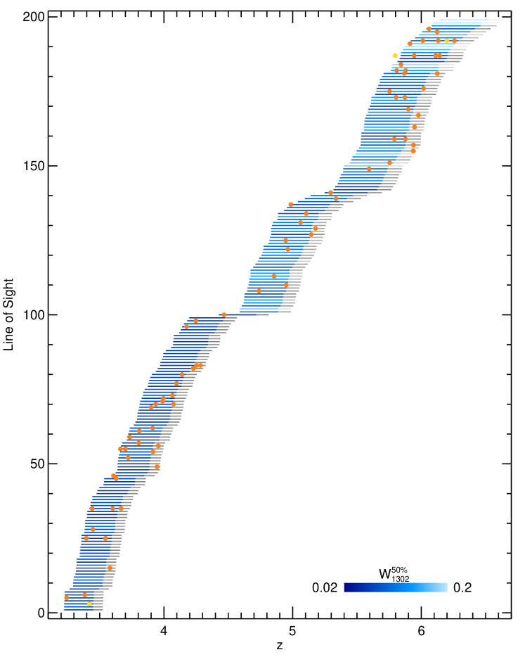
Figure 1: Summary of the survey results. The horizontal lines span the redshift interval over which each lines of sight was surveyed for O I. The grey shaded region on the right hand side of each line marks the proximate region within 5000 km s^-1 of the QSO redshift. The lines are shaded according to the 50% detection completeness limit in O I equivalent width. O I systems identified in our survey of ESI and X-Shooter spectra are marked with orange filled circles. The yellow circles in lines 187 (SDSS J0100+0524) and 191 (SDSS J1148+5251) are additional O I systems that were identified in Keck HIRES data only and are not part of our statistical sample. The yellow circle in line 3 (J1132+0052) is a probable O I system whose O I absorption is heavily blended, and is also not part of our statistical sample.

Each line of sight was surveyed for metal absorption systems traced by O I both visually and using the automated algorithm described in Section 3.3. The systems were identified via the coincidence of O I $\lambda$1302 in redshift with lines from other low-ionization metal ions, primarily Si II and C II. A detection required there to be significant absorption in O I $\lambda$1302 and either Si II $\lambda$1260 or C II $\lambda$1334. The velocity profiles were also required to be self consistent, taking into account occasional blends with unrelated absorption lines or contamination from strong skyline residuals. Both silicon and carbon should be mostly singly ionized in absorbers where hydrogen and oxygen are mostly neutral. Due to their higher ionization potentials, moreover, Si II (16.3 eV) and C II (24.4 eV) will tend to be ionized less easily than O I (13.6 eV). Our requirement that either Si II or C II be detected along with O I should therefore be robust to relative variations in line strength due to ionization. We could in principle miss systems due to large variations in relative abundances, but such variations are not generally seen (Cooke et al., 2011; Becker et al., 2012). In practice, both Si II $\lambda$1260 (in cases where it falls redward of the Ly$\alpha$ forest) and C II $\lambda$1334 were always detected along with O I $\lambda$1302. O I $\lambda$1302, Si II $\lambda$1260, and C II $\lambda$1334 tend to have comparable equivalent widths (though see Section 4). We also searched for weaker lines such as Si II $\lambda$1304 and Si II $\lambda$1526. These tend to be present for stronger systems but were not required for detections. Similarly, we included the Mg II $\lambda$$\lambda$2796,2803 doublet in systems for which we had the necessary wavelength coverage, but did not use these lines for the initial identification. We also measured the high-ionization doublets C IV $\lambda$$\lambda$1548,1550 and Si IV $\lambda$$\lambda$1393,1402 for detected O I systems as our wavelength coverage permitted.

Each line of sight was surveyed for O I systems between the QSO redshift and the redshift where O I $\lambda$1302 enters the Ly$\alpha$ forest. In all cases our spectra cover the primary low-ionization lines, including C II $\lambda$1334, up to the QSO redshift. The minimum redshift is defined as $1+z_{\rm min}=(1+z_{\rm forest})\lambda_{\rm Ly\alpha}/\lambda_{\rm O\,I}$, where $\lambda_{\rm Ly\alpha}$ and $\lambda_{\rm O\,I}$ are the rest-frame wavelengths of H I Ly$\alpha$ and O I $\lambda$1302, respectively, and $z_{\rm forest}$ is the redshift of the apparent start of the Ly$\alpha$ forest, determined visually for each line of sight (see Table 1). We note that $z_{\rm forest}$ is generally very similar to published values for the QSO emission redshifts. In our formal analysis we excluded “proximate” systems within 5,000 km s^-1 of $z_{\rm forest}$. The total redshift interval surveyed over $3.2<z<6.5$ is $\Delta z=57.7$ (76.5 including the proximity zones).

In order to more easily evaluate the evolution of O I systems with redshift, we generally quantify the survey pathlength in terms of an absorption pathlength interval $\Delta X$ (Bahcall & Peebles, 1969), defined as

$$\Delta X=\int_{z_{1}}^{z_{2}}(1+z)^{2}\frac{H_{0}}{H(z)}dz\,.$$ (1)

Here, $z_{1}$ and $z_{2}$ are the redshift bounds of the survey interval, and $H(z)$ is the Hubble parameter at redshift $z$. A non-evolving population of absorbers with constant comoving number density and proper cross-sectional area will have a constant line-of-sight number density $dn/dX$. Our total absorption pathlength interval is $\Delta X=250.1$ (332.7 including the proximity zones).

In total we detected 74 O I systems, 57 of which are separated from the QSO by more than 5000 km s^-1. A graphic depiction of the survey is shown in Figure 1. An additional system at $z=3.421$ towards J1332+0052 displays prominent low- and high-ionization lines; however, the O I $\lambda$1302 line itself is fully obscured by unrelated absorption lines. We therefore do not include it as part of our sample, even though it is probably an O I absorber. We note that the raw (not corrected for completeness) number densities of proximate and non-proximate absorbers are similar, $dn/dX\sim 0.2$ averaged over the entire redshift range. This contrasts with the enhanced number of high-ionization proximate absorbers typically seen along QSO lines of sight (e.g., Weymann et al., 1979; Nestor et al., 2008; Wild et al., 2008; Perrotta et al., 2016). A summary of the properties of each system is given in Table B. Line profiles are plotted in Figures 11–84.

3.2 Equivalent Width Measurements

We measured rest-frame equivalent widths ($W$) for up to eleven ionic transitions. For each system, a single velocity interval over which to integrate the absorption from low-ionization species (O I, C II, Si II, Mg II) was chosen via inspection of the line profiles. These intervals typically spanned less than 250 km s^-1 but extended up to 670 km s^-1 in some cases. A separate interval was chosen for the high-ionization lines (Si IV and C IV). When detected, the high-ionization lines often spanned a larger velocity interval than the low-ionization lines. In cases where no high-ionization lines are visually apparent, the equivalent widths for these lines were integrated over $\pm$100 km s^-1 of the nominal redshift of the low-ionization lines. We note that ESI and X-Shooter will generally not resolve the narrow ($b\lesssim 10$ km s^-1) components that are common for low-ionization absorbers, making it difficult to obtain column densities in many cases. We could in principle determine column densities for optically thin lines, or for species with multiple lines falling on different parts of the curve of growth. We chose to focus on equivalent widths, however, which are independent of resolution.

Blended lines were identified visually based on the line strength, velocity profile, and proximity of other absorption lines. We generally report the equivalent width for these systems as upper limits. For some mild blends, however, we measured an equivalent width after removing the blended line. For example, the O I $\lambda$1302 line at $z=3.804$ towards J1032+0927 is blended with C IV $\lambda$1550 at $z=3.034$ (Figure 26). In this case we inferred the C IV $\lambda$1550 profile by rescaling the C IV $\lambda$1548 line according to the ratio of the optical depths for these transitions. This pixel-by-pixel approach becomes problematic when the intervening lines are unresolved or optically thick. In general, however, we expect the de-blended equivalent widths to be accurate enough for the analysis considered below. Blending must also be considered in the case of doublets when the velocity extent of the absorption profile exceeds the doublet separation. We observed this in four cases for C IV ($z=3.7013$ towards J2215-1611, Figure 23; $z=3.8039$ towards J1032+0927, Figure 26; $z=3.9557$ towards J0835+0650, Figure 33; and $z=4.0742$ towards J0132+1341, Figure 37), but never in other doublets, for which the intrinsic velocity separation is larger. To correct this self-blending in C IV we used pixel-by-pixel optical depth rescaling to infer the portion of the blended profile from one transition from the corresponding un-blended portion of the other transition. That is, we calculated the red (blended) portion of the $\lambda$1548 profile from the red (unblended) portion of the $\lambda$1550 profile, and the blue (blended) portion of the $\lambda$1550 profile from the blue (unblended) portion of the $\lambda$1548 profile. Here again, although this procedure is not perfect, we do not expect the errors to significantly impact our analysis.

Notes on individual absorbers are given in Appendix B.

3.3 Completeness

We estimated our completeness by randomly inserting artificial absorption systems into the data and assessing whether they would be detected. The artificial absorbers were modeled as Voigt profiles convolved with the instrumental resolution, and were described by three parameters: a redshift, an O I column density, and a Doppler parameter. For each line of sight, 10⁴ absorbers were inserted in separate trials over the redshift interval where O I falls redward of the Ly$\alpha$ forest, matching our survey range. The O I column density was drawn randomly over the logarithmic interval $13<\log{(N_{\rm O\,I}/{\rm cm^{-2}})}<16$. The Doppler parameter was drawn randomly over the interval $b_{\rm min}<b<b_{\rm max}$, where $b_{\rm min}=10$ km s^-1and $b_{\rm max}$ increased linearly with $\log{N_{\rm O\,I}}$ from 10 km s^-1 at $\log{(N_{\rm O\,I}/{\rm cm^{-2}})}=13$ to 100 km s^-1 at $\log{(N_{\rm O\,I}/{\rm cm^{-2}})}=16$. These ranges in $\log{N_{\rm O\,I}}$ and $b$ were guided by Voigt profile fits to a selection of our observed systems, and were meant to roughly span the range in equivalent width and velocity width of the full observed sample. We note that a single Voigt profile does not capture the full kinematic complexity of many of the observed systems; however, the detectability of a system often depends on the strength of a dominant component. This is particularly true for weaker systems, for which completeness corrections are more important.

For each system we generated absorption lines in O I, C II, and Si II. The C II and Si II column densities were scaled from the O I values as $\log{N_{\rm C\,II}}=\log{N_{\rm O\,I}}-0.54$ and $\log{N_{\rm Si\,II}}=\log{N_{\rm O\,I}}-1.26$. These scalings were adopted from the relative abundances of metal-poor DLAs and sub-DLAs over $2\lesssim z\lesssim 4$ (Cooke et al., 2011; Dessauges-Zavadsky et al., 2003; Péroux et al., 2007) and O I systems at $z>5$ where column density measurements from high-resolution spectra are available (Becker et al., 2012).

We note that adopting fixed column density ratios ignores variations due to differences in relative abundance or, perhaps more significantly, ionization effects. As noted above, at a given O I equivalent width a partially ionized absorber will tend to have stronger Si II and C II than one that is fully neutral (in hydrogen), making it easier to detect. We argue below that the number density of O I absorbers is higher over $5.7<z<6.5$ than over $4.9<z<5.7$, a conclusion that depends partly on our completeness estimates. Assuming fixed column density ratios when determining completeness is conservative with respect to this conclusion in that if there are undetected weak O I absorbers with stronger Si II and/or C II, then the total O I number density should increase the most at $z>5.7$, where our sensitivity to weak systems is lowest. In practice, however, there is limited evidence for a large population of weak, partially ionized O I systems. The observed ratios of O I and C II equivalent widths tend to be near unity, particularly at $z>4.9$ (see Figure 8), with some exceptions noted below (Section 4).

In order to increase efficiency we used an automated detection algorithm for our completeness trials. The algorithm was developed to roughly mimic the process of identifying systems by eye, with detection criteria established using the real O I absorbers as a training set. The algorithm was also tested against by-eye identifications for artificial systems over the relevant range of absorber properties, spectral resolutions, and signal-to-noise ratios. Briefly, a detection required there to be significant absorption in O I $\lambda$1302 and at least one other line, and the kinematic profiles of the lines needed to be consistent with one another. The other lines examined were Si II $\lambda$1260, when it fell redward of the Ly$\alpha$ forest, and C II $\lambda$1334, which were the primary lines used when identifying O I systems visually.

For each of the 10⁴ artificial absorbers, the automated algorithm stepped across the nominal redshift in increments of 5 km s^-1 and examined the regions around the expected positions of each available line using the following steps. It first determined whether there was significant ($>$3$\sigma$) absorption after smoothing the spectrum by the instrumental resolution. If significant detection existed for all lines that fall redward of the Ly$\alpha$ forest then it fit a Voigt profile over $\pm$200 km s^-1 of that redshift independently to each available line. The continuum was allowed to vary by up to 5%, providing a mechanism to deal with small continuum errors as well as with nearby weak absorption lines. The flux cross-correlation between each pair of lines was also computed over the same velocity interval. In all cases, a detection required that, for at least two lines, the FWHM of the fitted profiles agreed to within a factor of 1.5, the equivalent widths of the fits agreed to within a factor of 4.0, and the ratio of the maximum absorption depths to the FWHM (in km s^-1) of the fits were greater than 0.002. The last condition was meant to reject spurious wide, weak lines. A detection was recorded if the centroids of the fits aligned to within 5 km s^-1, the FWHM of both Voigt profile fits were less than 200 km s^-1, and the reduced $\chi^{2}$ of the fits over the central FWHM were less than 5.0. Alternatively, a detection was recorded if the centroids of the Voigt profile fits aligned to within 30 km s^-1and the cross-correlation was greater than 0.75.

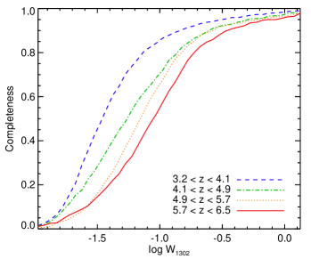
Figure 2: Survey completeness as a function of O I $\lambda$1302 equivalent width. Our four redshift intervals are plotted with the line styles indicated.

Our completeness estimates as a function of O I equivalent width are plotted in Figure 2. For each redshift bin we computed the pathlength-weighted mean completeness of all contributing lines of sight, excluding the redshift intervals immediately around known O I systems. As expected, the completeness tends to decrease with increasing redshift. This is largely driven by a decrease with redshift in the typical $S/N$ of our spectra (see Table 1). The increased number of strong residuals from sky emission line subtraction and telluric absorption correction towards redder wavelengths also contributes to this trend.

We expect some error in our completeness estimates due to the challenge of designing an automated detection algorithm that is robust to the inherent variations in real O I absorbers. The abundance ratios of different ions in these systems are not necessarily constant, and their kinematic profiles do not always perfectly match (for example, C II can have components not present in O I due to ionization effects; see discussion above). We nevertheless believe that errors in our completeness estimates are not strongly affecting our results. Out of the 74 real systems identified visually, the automated algorithm identified 68 (92%). Of the six systems missed, two have O I $\lambda$1302 equivalent widths below the cutoff of $W_{1302}>0.05$ Å we impose for the analysis in Section 3.4. The remaining four were readily identified by eye but were missed by the automated algorithm due to complexities in the line profiles or the presence of nearby strong lines, which caused the algorithm to fail in some cases. Of these four, three had $W_{1302}>0.2$ Å, where our completeness estimate is $>$80% at all redshifts (Figure 2). The remaining system was one out of 32 real O I systems in the range $0.05~{}{\rm\AA}<W_{1302}<0.20~{}{\rm\AA}$, where the completeness corrections are more significant. We therefore expect the overall errors in our completeness estimates to be small compared to the statistical errors described below. Completeness corrections are discussed further in Section 3.5.

False positive detections should only be a minor concern for this work. In principle there can be false detections from the chance alignment of unrelated lines. In practice, however, although we used only O I $\lambda$1302, Si II $\lambda$1260, and C II $\lambda$1334 to visually identify O I absorbers, nearly all of our systems were detected in at least three lines. If Si II $\lambda$1260 fell in the Ly$\alpha$ forest, then Si II 1304 and Si II $\lambda$1526 were generally available, or the system was detected in Mg II or higher ionization lines (Si IV and/or C IV). In the single case where the system was only detected in O I $\lambda$1302 and C II $\lambda$1334 (the $z=5.7533$ system towards SDSS J2315-0023, Figure 59), the asymmetric kinematic profiles are distinct enough that a false positive from unrelated lines is unlikely. We therefore expect that essentially all of our O I detections are genuine.

3.4 Equivalent Width Distributions

Our primary goal is to determine how the number density of O I systems evolves with redshift. In order to extend this analysis to equivalent widths where we are significantly incomplete, we need to adopt a functional form for the distribution of equivalent widths. Exponential and power law distributions are commonly adopted for metal lines (see also the Schechter function used by Mathes et al. (2017) and Bosman et al. (2017)). Here we adopt an exponential distribution, which we find provides a reasonable fit to the observed distribution. We note, however, that our final conclusions do not depend sensitively on this choice. We repeated the analysis below using a power law fit to the equivalent width distribution and obtained very similar results for the integrated number density.

We fit an exponential distribution of the form

$$f(W)=\frac{\partial^{2}n}{\partial W\partial X}=\frac{A}{W_{0}}e^{-W/W_{0}}\,,$$ (2)

where $W_{0}$ is the exponential cutoff scale and $A$ is the number density per unit pathlength $X$ integrated over $0<W<\infty$. $A$ and $W_{0}$ were fit simultaneously in four redshift bins using a maximum likelihood approach similar to the one described in Bosman et al. (2017). We used a forward modeling approach in which likelihood values were derived from the model intrinsic $f(W)$ multiplied by our completeness (Figure 2). We divided our survey into roughly equal bins in redshift: $3.2<z<4.1$, $4.1<z<4.9$, $4.9<z<5.7$, and $5.7<z<6.5$ (but see Appendix A). These bins contain 18, 5, 8, and 18 intervening systems with $W_{1302}>0.05$ Å, respectively. In order to minimize our statistical uncertainties while limiting our sensitivity to large completeness corrections we only fit over equivalent widths where we are $>$25% complete at all redshifts, $W_{1302}>0.05$ Å. We comment further on this choice below.

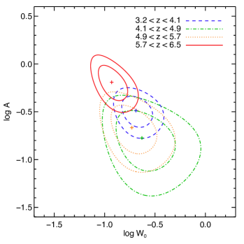
Figure 3: Results of the exponential fit to the distribution of O I $\lambda$1302 equivalent widths for $W_{1302}>0.05$ Å. The contours show the 68% and 95% likelihood bounds over each redshift interval for the parameters in Equation 2. Crosses mark the highest probability values.

Table 2: Summary of results

$z$	$\Delta X$	$n$	$\log{A}$	$\log{W_{0}}$	$dn/dX$
3.2–4.1	79.0	28,22,18	$-0.49^{+0.09}_{-0.13}$	$-0.69^{+0.11}_{-0.09}$	$0.255^{+0.057}_{-0.061}$
4.1–4.9	44.1	9,6,5	$-0.77^{+0.16}_{-0.26}$	$-0.63^{+0.24}_{-0.15}$	$0.136^{+0.059}_{-0.059}$
4.9–5.7	62.5	11,9,8	$-0.67^{+0.13}_{-0.20}$	$-0.73^{+0.17}_{-0.13}$	$0.165^{+0.055}_{-0.058}$
5.7–6.5	66.3	26,20,18	$-0.19^{+0.10}_{-0.14}$	$-0.93^{+0.11}_{-0.08}$	$0.421^{+0.098}_{-0.101}$

Note. — Columns: (1) QSO index number, (2) QSO name, (3) QSO redshift based on the apparent start of the Ly$\alpha$ forest, (4) instrument used for the O I search, (5) signal-to-noise ratio per 30 km s^-1 near rest wavelength 1285 Å, (6) O I $\lambda$1302 rest-frame equivalent width, in angstroms, at which the O I search is 50% complete.

Note. — Columns: (1) redshift range, (2) absorption pathlength interval, (3) number of O I systems: total, non-proximate, and non-proximate with $W_{1302}>0.05$ Å, (3) constraints on $\log{A}$, (4) constraints on $\log{W_{0}}$, where $W_{0}$ is in Å, (5) constraints on $dn/dX$. All constraints are for O I systems with $W>0.05$ Å. Errors are marginalized 68% confidence intervals. The errors in $\log{A}$ and $\log{W_{0}}$ are correlated (Figure 3).

Our likelihood contours are shown in Figure 3, and the results are summarized in Table 2. For all redshifts there is a degeneracy between $A$ and $W_{0}$. The fits are least constrained over $4.1<z<4.9$ and $4.9<z<5.7$, where there are the fewest detections. These bins are consistent with a similar cutoff but lower normalization than $3.2<z<4.1$, although the uncertainties are significant. Over $5.7<z<6.5$ our fits prefer a somewhat lower cutoff and a higher normalization. The 95% confidence intervals overlap between the highest and two middle redshift bins. Overall, however, there is evidence that equivalent width distribution evolves with redshift, which we explore further below.

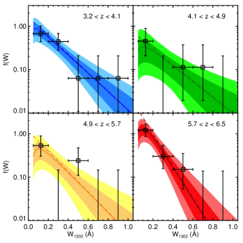
Figure 4: Binned O I $\lambda$1302 equivalent width distributions. Bins containing detected systems are plotted with squares and two-sided 68% Poisson confidence intervals. Non-detections are shown with one-sided 84% upper limits. The data are not corrected for completeness. The dark and light shaded regions in each panel show the 68% and 95% confidence intervals to the exponential fit, derived from the likelihood distributions in Figure 3 and multiplied by the completeness functions in Figure 2. Dashed and solid lines show the best fitting exponential distributions before and after multiplying by the completeness functions, respectively.

In Figure 4 we compare our fits to the observed equivalent width distributions in bins of $W_{1302}$. Confidence intervals for $f(W)$ were determined by sampling the full posterior distribution for $A$ and $W_{0}$. We do not correct the binned data for completeness, which requires knowing the underlying shape of the distribution. Instead, we multiply the model fits by our completeness estimates. We emphasize that Figure 4 is for visualization only; the parameters for $f(W)$ were fit to the unbinned data. Nevertheless, it shows that our choice of an exponential distribution gives a reasonable fit to the data.

3.5 Number Density

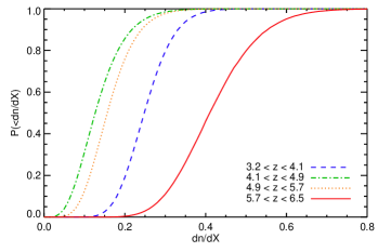
Figure 5: Cumulative probability distributions for the comoving number density of O I systems with $W_{1302}>0.05$ Å. The distributions were computed by integrating Equation 2, marginalizing over the parameter distributions in Figure 3.

Figure 6: Comoving number density of O I systems with $W_{1302}>0.05$ Å as a function of redshift. The results were obtained by integrating Equation 2 using the parameter distribution shown in Figure 3. Filled symbols show the most likely values at each redshift. Vertical errors bars show the 68% confidence intervals taken from Figure 5. Results for smaller redshift bins are shown in Figure 10.

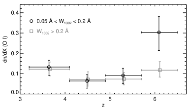
Figure 7: Comoving number density of O I systems as a function of redshift, divided into equivalent width ranges. The results were obtained by integrating Equation 2 using the parameter distribution shown in Figure 3. Circles show the most likely values for systems with $0.05~{}{\rm\AA}<W_{1302}<0.2~{}{\rm\AA}$, while squares are for $W_{1302}>0.2~{}{\rm\AA}$. Vertical errors bars show the 68% confidence intervals. Points are slightly offset in redshift for clarity

We now turn to computing the integrated line-of-sight number density of O I systems as a function of redshift. In each redshift bin we computed $dn/dX$ by integrating Equation 2 over $W_{1302}\geq 0.05$ Å, the range over which $f(W)$ was fit. We constructed a probability distribution for $dn/dX$ from the full posterior distributions for $A$ and $W_{0}$ shown in Figure 3. The cumulative distributions for our four redshift bins are shown in Figure 5.

In Figure 6 we plot the most probable values and 68% confidence intervals for $dn/dX$ as a function of redshift. The results are summarized in Table 2. The evolution over $3.2<z<4.9$ is consistent with a moderate increase with decreasing redshift. This is the expected behavior if the number density of O I systems is driven mainly by the ongoing metal enrichment of the CGM with time. The number densities over $4.1<z<4.9$ and $4.9<z<5.7$ are similar, albeit with significant uncertainties. The number density over $5.7<z<6.5$, however, is notably higher than over $4.9<z<5.7$. Using the cumulative probability distributions plotted in Figure 5, we find that $dn/dX$ over $5.7<z<6.5$ is a factor of $2.5^{+1.6}_{-0.8}$ greater than over $4.9<z<5.7$ at 68% confidence, with a probability that the $dn/dX$ is larger at $z>5.7$ of 98.9%. This increases to 99.7% if we compare $dn/dX$ over $5.7<z<6.5$ to that inferred from a single fit to $f(W)$ over $4.1<z<5.7$. This decline with decreasing redshift runs contrary to the naive expectation that the number density of O I systems should monotonically trace the buildup of CGM metals with time.

In Figure 7 we divide the $dn/dX$ results into two equivalent width ranges, $0.05~{}{\rm\AA}<W_{1302}<0.2~{}{\rm\AA}$ and $W_{1302}>0.2~{}{\rm\AA}$. We caution that the values in Figure 7 were calculated using the fits to Equation 2 computed over the full equivalent width range ($W_{1302}>0.05$ Å; Figure 3), rather than from separate fits over these smaller ranges. Nevertheless, the results demonstrate how the shape of $f(W)$ evolves with redshift. In the three redshift bins over $3.2<z<5.7$ the number density of systems in the two $W_{1302}$ ranges is roughly equal. Over $5.7<z<6.5$, however, the number density of systems with $0.05~{}{\rm\AA}<W_{1302}<0.2~{}{\rm\AA}$ is a factor of $\sim$3 higher than those with $W_{1302}>0.2~{}{\rm\AA}$. The number density of stronger systems is nominally somewhat lower over $4.1<z<5.7$ that at $z>5.7$, but is consistent within the 68% confidence intervals with no evolution over the entire redshift range studied. Most of the evolution occurs among the weaker systems, where $dn/dX$ declines by a factor of $3.3^{+2.8}_{-1.2}$ (68% confidence) from $5.7<z<6.5$ to $4.9<z<5.7$.

As noted above, our results depend partly on completeness corrections, which increase towards smaller values of $W_{1302}$. For the best fits to $f(W)$ in Table 2, our total corrections on $dn/dX$ for $W_{1302}>0.05$ Å are factors of 1.2 over $3.2<z<4.1$, 1.4 over $4.1<z<4.9$, 1.5 over $4.9<z<5.7$, and 1.9 over $5.7<z<6.5$. We can test whether our results may be driven by errors in the completeness estimates by varying the range in $W_{1302}$ over which we fit $f(W)$. Increasing or decreasing the minimum $W_{1302}$ by a factor of two produces nominal values for $A$ and $W_{0}$ that are well within the 68% uncertainties in Figure 3. The more conservative limit of $W_{1302}>0.1$ Å gives a minimum completeness of $>$55% at all redshifts (Figure 2), and smaller total completeness corrections for the nominal values of $dn/dX$, factors of 1.1, 1.2, 1.2, and 1.4 in order of increasing redshift. We nevertheless recover the same trends in $dn/dX$ for $W_{1302}>0.1$ Å, albeit at somewhat lower statistical significance; a decrease in $dn/dX$ from $5.7<z<6.5$ to $4.9<z<5.7$ is still favored at 96% confidence. Our results therefore do appear to be driven by errors in the completeness estimates for small values of $W_{1302}$.

We discuss the implications of the evolution in $dn/dX$ below, but first examine the high-ionization metal species associated with our O I absorbers.

4 High-Ionization Components

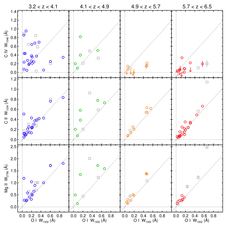
Figure 8: C IV $\lambda$1548 (top row), C II $\lambda$1334 (middle row), and Mg II $\lambda$2796 (bottom row) equivalent widths as a function of O I $\lambda$1302 equivalent width for the systems in our survey. The sample is divided into redshift bins as indicated along the top. In each panel we plot only cases where measurements were obtained for both ions. Downward arrows are 2$\sigma$ upper limits on non-detections. 68% errors bars are shown when they are larger than 0.05 Å. In some cases, points with error bars were measured from noisy data where there is visually no obvious detection, and should therefore be treated with caution. Light grey squares denote proximate absorbers. The diagonal line in each panel shows where the two ions have equal equivalent widths in dimensionless units.

In the top panels of Figure 8 we compare the rest-frame equivalent widths of the high-ionization line C IV $\lambda$1548 to O I $\lambda$1302 for our detected O I systems. The diagonal dotted line in each panel represents equal C IV and O I equivalent widths in dimensionless units (i.e., with the rest-frame wavelengths factored out). A clear trend of increasing C IV strength towards lower redshifts is seen. All of the O I systems at $z<4.9$ have detected C IV, and for a large majority of these the C IV absorption is similar to or stronger than O I. At $z>4.9$, in contrast, C IV is typically weak or not detected. In some cases with high-$S/N$ data (e.g., the $z=6.1115$ and 6.1436 systems towards SDSS J010+2802, Figures 79 and 83) the 3$\sigma$ upper limits on C IV are extremely low ($W_{1548}<0.005$ Å). Similar results were found by Cooper et al. (2019).

We note that where high-ionization components are detected they tend not to align kinematically with O I. In cases where they can be clearly identified, the C IV and Si IV components are often broader, more numerous, and/or offset in velocity from O I. As others have noted (e.g., Fox et al., 2007), this implies that, in many cases, O I and C IV are likely to arise from separate phases of the CGM. This potentially complicates the role that high-ionization lines can play in interpreting the redshift evolution of O I, a point we return to below.

For comparison, we also compare the low-ionization transitions C II $\lambda$1334 and Mg II $\lambda$2796 to O I in Figure 8. Here there is noticeably less redshift evolution. In the large majority of systems, the rest-frame equivalent widths (in dimensionless units) of C II and Mg II are comparable to O I. Cases where $W_{1334}$ and $W_{2796}$ are substantially higher than $W_{1302}$, which mainly occur at $z<4.9$, are likely to be partially ionized absorbers. This is reflected in the fact that absorption components with strong C II compared to O I also tend to appear in Si IV and C IV (e.g., the components at $\Delta v\simeq 60$ and 170 km s^-1 in the $z=3.3844$ system towards J1018+0548, Figure 12; and the $z=3.6287$ system towards J0042-1020, Figure 20).

Finally, we note that proximate absorbers (light grey squares in Figure 8) show similar trends in the relative strength of high- and low-ionization lines as non-proximate absorbers. This suggests that many of the proximate absorbers may be far enough away from the background QSO that ionizing radiation from the QSO does not strongly affecting the ionization balance, in contrast with the trends seen for absorbers selected via C IV (Perrotta et al., 2016). Alternatively, the similarity may result from a combination of trends in metallicity and ionization that are a function of proximity to the background QSO (e.g., Ellison et al., 2010, 2011).

5 Potential Clustering of O I Absorbers

A notable feature of Figure 1 is that detections of multiple O I systems along a single line of sight seem to be more common near $z\sim 6$ than at lower redshifts. This was previously seen by Becker et al. (2006) in the case of SDSS J1148+5251, which contains four O I systems within a span of $\Delta z=0.25$ (100 comoving Mpc). The weakest of these, marked by a yellow circle in Figure 1, is detected only in high-resolution Keck HIRES data (Figure 6 of Becker et al., 2011). Here we find that SDSS J0100+2802 also contains four O I systems over a similar interval ($\Delta z=0.31$, 130 comoving Mpc). The redshift of one of these, $z=5.7975$, falls just below our nominal survey pathlength for this object and is not included in the statistical sample. The O I line falls in the proximity zone region of the Ly$\alpha$ forest but is clearly identified by its narrow width in HIRES data (Figure 85). Three other $z\sim 6$ lines of sight (SDSS J0818+1722, CFHQS J2100-1715, and PSO J3008-21) contain two O I systems outside the proximity zone. In contrast, multiple detections outside the proximity zone are seen towards only two lower-redshift QSOs (J1108+1209 and J2215-1611).

We caution that this apparent increase in O I multiplicity with redshift could be misleading for two reasons. First, the redshift interval $\Delta z$ between the edge of the proximity zone and the redshift where O I $\lambda$1302 enters the Ly$\alpha$ forest increases with redshift. This can be seen as a lengthening of the survey paths towards higher redshift in Figure 1. In addition, the absorption pathlength per unit redshift, $dX/dz$, also increases with redshift (Equation 1). The combination of these factors means that the absorption pathlength interval $\Delta X$ over which we searched for O I is a factor of 1.7 larger for a QSO at $z=6$ than for one at $z=4$. This may partially explain the greater incidence rate of multiple detections towards higher redshifts.

It is nevertheless worth examining whether the O I systems near $z\sim 6$ are clustered. Some amount of clustering at any redshift is naturally expected due to galaxy clustering. If, as we propose below, the incidence of O I at $z>5.7$ is higher than at lower redshift because of a lower ionizing UVB, then additional clustering at these redshifts may be expected if there are also fluctuations in the UVB amplitude (e.g., Finlator et al., 2015). UVB fluctuations may indeed be present, as they are broadly expected near the tail end of reionization (e.g., Mesinger & Furlanetto, 2009; Crociani et al., 2011; McQuinn et al., 2011; Davies & Furlanetto, 2016; Finlator et al., 2018; D’Aloisio et al., 2018; Kulkarni et al., 2019; Keating et al., 2019), and may be driving the large observed scatter in IGM Ly$\alpha$ opacity near $z\sim 6$ (Fan et al., 2006; Becker et al., 2015; Bosman et al., 2018; Eilers et al., 2018).

Here we focus on whether there is significant evidence for clustering, leaving a more sophisticated analysis of the underlying correlation function for future work. We tested the null hypothesis of no clustering, where O I systems are distributed randomly along the QSO lines of sight, using a Monte Carlo approach to generate mock data sets. In each of $10^{5}$ trials we assigned a random number of systems along each line of sight drawn from a Poisson distribution with a mean value equal to $\Delta X$ for that line of sight multiplied by the number density expected from integrating over the best-fitting equivalent width distribution $f(W)$ for $5.7<z<6.5$ ($\log{W_{0}}=-0.93$ and $\log{A}=-0.19$; Table 2). We integrated down to $W_{1302}=0.02$ Å, or somewhat lower than the weakest O I detection in our statistical sample. The systems were assigned equivalent widths by randomly drawing from the $f(W)$ distribution, and random redshifts within the survey interval for each QSO. We then randomly determined whether the systems were detected using the completeness function for that QSO. We found that at least five lines of sight yielded at least two O I detections at $z>5.7$, similar to the observed data, in 18% of trials. Two or more lines of sight yielded three or more O I detections at $z>5.7$, similar to SDSS J1148+5251 and SDSS J0100+2802, in 7% of the trials. There is therefore some hint that O I systems at $z\sim 6$ may be clustered, although this test does not strongly rule out the null hypothesis of no clustering. Stronger constraints may come from a larger and/or more sensitive survey.

6 Discussion

In this section we consider the implications of our observations for the evolution of metal-enriched circumgalactic gas. Two facts about O I systems are apparent from the data:

1. The number density of O I systems is substantially (a factor of $\sim$2–4) lower over $4.1<z<5.7$ than over $5.7<z<6.5$.

2. Over the redshift range of this study ($3.2<z<6.5$), O I systems show increasing amounts of C IV absorption towards lower redshifts.

The first point contrasts with the overall trend of metal enrichment expected for the CGM, namely that the metal content of circumgalactic gas should increase with time as metals are driven into the CGM by galactic outflows. If the ionization balance of these metals remained constant with time, therefore, we would expect the number density of all species, including O I, to increase with decreasing redshift. The fact that O I decreases at $z<5.7$ presumably then means that a substantial fraction of the circumgalactic metals are transitioning from a relatively neutral state to higher ionization states where O I is less favored. In other words, the CGM of galaxies at $z\sim 6$ appears to be undergoing reionization.

The fact that the ionization transition at $z\sim 6$ is relatively rapid (see also Appendix A) suggests that circumgalactic metals are generally ionized by an external radiation field. There are no obvious changes in the global properties of galaxies at that epoch that would rapidly drive inside-out ionization of the CGM. The evolving meta-galactic radiation field during or shortly after reionization is a more likely culprit. Indeed, the intensity of hydrogen ionizing background is inferred to increase by roughly an order of magnitude from $z\sim 6$ to 5 based on measurements of the opacity of the Ly$\alpha$ forest (Wyithe & Bolton, 2011; Davies et al., 2018) and the extent of QSO proximity zones (Calverley et al., 2011). As shown in Figure 7, we find that much of the evolution in O I absorbers near $z\sim 6$ occurs among weaker systems ($W_{1302}<0.2$ Å). The weaker O I systems may be more sensitive to changes in the UVB if they correspond to lower-density gas.

The reionization of the metal-enriched CGM may occur contemporaneously with reionization of the surrounding IGM as an ionization front sweeps through. Alternatively, the circumgalactic gas, being more dense, may remain self-shielded for some time after the local IGM becomes ionized. In the latter case the CGM would become increasingly ionized as the surrounding UV background strengthens. This should occur near the tail end of reionization as the local mean free path of ionizing photons increases, exposing a given region to ionizing photons from more distant sources (e.g., Mesinger & Furlanetto, 2009; Crociani et al., 2011; McQuinn et al., 2011). In either case, the reionization of the CGM should be coupled to the reionization of the IGM. Careful modeling is needed to precisely constrain the timing of IGM reionization using metal absorption lines (e.g., Keating et al., 2014; Finlator et al., 2015, 2018, Doughty, in prep.). Broadly speaking, however, the observed evolution in O I suggests that a significant phase of intergalactic—as well as circumgalactic—reionization may have occurred at or not long before $z\sim 6$.

The evolution of C IV in our O I systems supports a picture in which highly ionized metals make up a larger proportion of circumgalactic metals towards lower redshifts. While some O I absorbers at $z\sim 6$ must transition to more highly ionized states at lower redshifts, however, it is not obvious that a large fraction of the gas producing O I absorption at $z\sim 6$ produces C IV absorption at $z<5$. For a C/O number density ratio of 0.3, typical of low-metallicity DLAs and high-redshift O I systems (Cooke et al., 2011; Becker et al., 2012), a fully neutral absorber with O I $\lambda$1302 optical depth $\tau_{1302}=1.0$ that becomes ionized will have a C IV $\lambda$1548 optical depth $\tau_{1548}=1.4$ (i.e., easily detectable) if half of the carbon is in C IV. The C IV fraction will depend on the gas density and the spectrum of the ionizing radiation, however, and may be much lower (e.g., Simcoe, 2011). It is possible that some $z\sim 6$ O I systems become mildly ionized absorbers that appear in C II, Si II, and/or Mg II but not O I. The O I systems may also initially become absorbers dominated by C III and Si III, whose transitions fall in the heavily absorbed Ly$\alpha$ forest. In any case, the evolutionary link between O I at $z\sim 6$ and C IV at lower redshifts is unclear. The buildup of C IV in O I absorbers with time may simply reflect the ongoing enrichment of the CGM, with C IV at $z<5$ largely tracing metals that were not yet in place at $z\sim 6$.

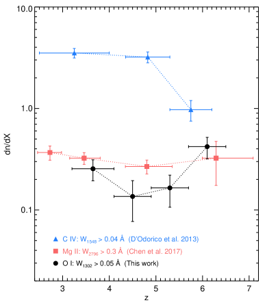
Figure 9: Number density of O I (circles), Mg II (squares), and C IV (triangles) systems over $3\lesssim z\lesssim 7$ down to current equivalent width limits. Vertical error bars are 68% confidence intervals. The results for O I systems with $W_{1302}>0.05$ Å are from this work. Results for Mg II systems with $W_{2796}>0.3$ Å are from Chen et al. (2017). The C IV results for systems with $W_{1548}>0.04$ Å were derived from D’Odorico et al. (2013) (see also Codoreanu et al., 2018). See text for details.

In Figure 9 we summarize the number density evolution of multiple ions from different surveys out to $z\sim 7$. The results for Mg II systems with Mg II $\lambda$2796 equivalent width $W_{2796}>0.3$ Å are from Chen et al. (2017). For C IV we integrated the column density distributions from D’Odorico et al. (2013) over $\log{(N_{\rm C\,IV}/{\rm cm^{-2}})}>13.0$, and converted the lower bound in column density into a C IV $\lambda$1548 equivalent width limit of $W_{1548}>0.04$ Å assuming Doppler parameters $b>10$ km s^-1. The rise in C IV from $z\sim 6$ to 5 (similar to that found by Codoreanu et al., 2018) contrasts with the drop in O I over the same redshifts, while Mg II remains relatively flat.

We caution that the equivalent width limits in Figure 9, which are generally set by the quality of the data at the highest redshifts, may complicate the comparison of different ions. For example, the number density of O I systems we measure at $z\sim 6$ is nominally somewhat higher than the number density of Mg II systems found by Chen et al. (2017), but this may be due to differences in sensitivity. For an absorber with a column density ratio $N_{\rm O\,I}/N_{\rm Mg\,II}$ equal to the solar O/Mg ratio (Asplund et al., 2009), an optically thin system would have an Mg II $\lambda$2796 equivalent width, in angstroms, roughly twice that of O I $\lambda$1302. In that sense the Chen et al. (2017) limit of $W_{2796}>0.3$ is only a factor of $\sim$3 above our O I limit of $W_{1302}>0.05$ Å for weak low-ionization systems. According to our best fit to Equation 2, increasing our O I limit by a factor of three, from $W>0.05$ Å to $W>0.15$ Å, would yield a factor of $\sim$2 fewer O I systems at $z\sim 6$, i.e., somewhat lower than the number density of Mg II systems with $W_{2796}>0.3$ Å found by Chen et al. (2017) though still within the error bars. There may be significant numbers of weak Mg II absorbers at $z\sim 6$ without O I, but further work will be needed to determine whether this is the case. Bosman et al. (2017) found that an abundant population of Mg II systems at $z\sim 6$ may exist below the detection limit of Chen et al. (2017), although the evidence comes from only one line of sight.

We also emphasize that the number densities plotted in Figure 9 are dominated by the weakest systems, and do not necessarily reflect the evolution in the total mass density. A more comprehensive picture would come from examining how the full equivalent width (or column density) distributions of these ions evolve with redshift. Nevertheless, these trends should already place strong constraints on models of CGM enrichment and ionization.

Finally, we briefly comment on two possible implications of our O I results for the radiation emitted from high-redshift galaxies. The higher O I number density at $z>5.7$ implies that, globally, the mean projected cross-section of largely neutral, optically thick gas around galaxies is higher at $z\gtrsim 6$ than at $z\sim 4$–5. This could imply a smaller escape fraction of ionizing photons at $z\sim 6$ compared with lower redshifts, at odds with reionization models that require higher average escape fractions at higher redshifts (e.g., Kuhlen & Faucher-Giguère, 2012; Haardt & Madau, 2012). On the other hand, ionizing photons may largely escape from a galaxy’s interstellar and circumgalactic media through channels of low H I column density (e.g., Ma et al., 2016; Steidel et al., 2018). The number of such channels will depend on the three-dimensional geometry of the optically thick gas (e.g., Fernandez & Shull, 2011), which can vary for a given two-dimensional cross-section. The hosts of O I absorbers and the galaxies that dominate the ionizing emissivity may also be separate populations. A higher global cross-section of neutral gas could also have implications for galaxy Ly$\alpha$ emission. If a significant fraction of the Ly$\alpha$ emission from a galaxy is scattered within optically thick regions of the CGM (e.g., Rauch et al., 2008; Steidel et al., 2011; Wisotzki et al., 2018), then a larger neutral cross-section could potentially correspond to a more extended, lower surface brightness Ly$\alpha$ halo. This would make galaxy Ly$\alpha$ emission more difficult to detect, and could be partially responsible for the lower fraction of galaxies that appear as Ly$\alpha$ emitters at $z>6$ (e.g., Hoag et al., 2019; Mason et al., 2019, and references therein). The significance of these effects is difficult to determine without further study.

7 Summary

We conducted a survey for metal absorbers traced by O I over $3.2<z<6.5$. Using moderate-resolution spectra of a 199 QSOs, we find that the number density of systems with O I equivalent width $W_{1302}>0.05$ Å decreases by a factor of $2.5^{+1.6}_{-0.8}$ (68% confidence) from $5.7<z<6.5$ to $4.9<z<5.7$, with a decrease at some level favored with 99% confidence. Much of the decline occurs among weak ($W_{1302}<0.2$ Å) absorbers. The number density then inflects towards an increasing trend with decreasing redshift over $3.2<z<5.7$.

The decrease in O I at $z<5.7$ runs contrary to the general expectation that the overall metal content of circumgalactic gas should increase with time, and implies that metal-enriched gas at $z\sim 6$ tends to be in a more neutral state compared to lower redshifts. Supporting this picture, we find that the amount of absorption by highly ionized metals traced by C IV associated with O I systems increases with decreasing redshift (see also Cooper et al., 2019).

Our O I results suggests that the metal-enriched gas around galaxies undergoes an ionization transition near $z\sim 6$ driven by a strengthening metagalactic ionizing background. Such an increase in the UVB is expected near the end of hydrogen reionization. The reionization of the CGM seen in O I therefore adds to the growing observational evidence that the reionization of the IGM may have been ongoing or had only recently ended at $z\sim 6$. The evolution in the CGM neutral fraction may also carry implications for the Lyman continuum and/or Ly$\alpha$ emission from galaxies at $z\gtrsim 6$.

Further observations of O I and other ions will help to clarify how metal enrichment and ionization proceed near reionization. Larger surveys would help to determine the rate at which circumgalactic metals undergo the ionization transition detected here near $z\sim 6$. More sensitive data at $z>5$ would give further insight into the weak O I systems that seem to evolve the most strongly. Finally, pushing the search for O I and other metals to even higher redshifts would help to better understand the connection between the evolution of the CGM and the reionization of the IGM. The growing number of QSOs being discovered at $z>7$ (e.g., Bañados et al., 2017) should make this possible.

Appendix A Alternate Redshift Binning

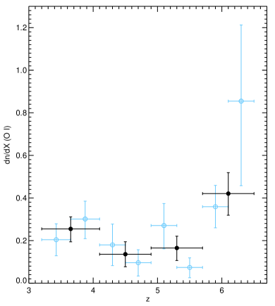
Figure 10: Comoving number density of O I systems with $W_{1302}>0.05$ Å as a function of redshift. Filled circles are the same as in Figure 6 and use bin sizes $\Delta z=0.8$–0.9. Open circles use redshift bins $\Delta z=0.4$–0.45.

In this appendix we explore the use of smaller redshift bins for tracing the number density of O I systems. We repeated the procedure described in Sections 3.4 and 3.5, but divided each of our nominal redshift bins into two such that the bins sizes are $\Delta z=0.45$ over $3.2<z<4.1$ and $\Delta z=0.4$ over $4.1<z<6.5$. The $dn/dX$ results for absorbers with $W_{1302}>0.05$ Å are shown in Figure 10. Over $3.2<z<5.7$ we see the same general trend of a flat or increasing number density with decreasing redshift, albeit with larger errors. There is some evidence that the decline with decreasing redshift near $z\sim 6$ may be steeper than suggested by the $\Delta z\simeq 0.8$ bins. This comes primarily from the high nominal value of $dn/dX$ at $z=6.3$, though the uncertainty on this point is large. There are five O I systems over $6.1<z<6.5$ in our statistical sample, all of which have $W_{1302}<0.17$ (although the proximate system at $z=6.1242$ towards PSO J065-26 has $W_{1302}\simeq 0.7$). Completeness corrections are necessarily large in this bin, a factor of 3.2 overall in $dn/dX$ for the nominal fit to $f(W)$. With such a small sample it is also unclear whether a single exponential is a reasonable model for $f(W)$. While the finer redshift binning gives some hint that the evolution near $z\sim 6$ may be even more substantial than indicated by the nominal $\Delta z\simeq 0.8$ bins, therefore, the results push the limits of what can be learned from the current data. More detailed constraints on O I evolution at these redshifts will require a larger and/or more sensitive survey.

Appendix B Details on Individual Systems

Here we provide more detailed information on individual absorption systems. The systems are plotted in Figures 11–84. Solid shading marks the region over which an equivalent width was integrated. Hatched shading denotes lines that are either blended with an unrelated absorber or contaminated by strong telluric residuals.

Equivalent width measurements for all ions are given in Table B. Notes on individual systems are given below. Blended lines are mentioned in the notes only in cases where a correction for blending has been made (see Section 3.2) or the blend is questionable. Other blends are reported in Table B as upper limits on the equivalent width.

• $z=3.6287$ towards J0042-1020 (Figure 20): O I $\lambda$1302 is extremely weak compared to C II $\lambda$1334 and Si II $\lambda$1526, an indication that the gas traced by the low-ionization lines is significantly ionized in this system. Among the XQ-100 lines of sight, this is the only intervening (not proximate) absorber not identified as a DLAs or sub-DLA (Sánchez-Ramírez et al., 2016; Berg et al., 2016, and in prep).

• $z=3.7013$ towards J2215-1611 (Figure 23): This system exhibits self-blending in C IV. Deblended equivalent widths measured are reported in Table B. We note that Mg II and the high-ionization lines exhibit two extended ($\Delta v\sim 100$ km s^-1) components separated by 500 km s^-1, which is very similar to the intrinsic C IV doublet separation. A similar separation is seen in the C IV components of the $z=3.9557$ towards J0835+0650 (Figure 33). Although it may occur by chance, this separation is reminiscent of a line-locking signature sometimes seen in radiately driven outflows (e.g., Milne, 1926; Scargle, 1973; Bowler et al., 2014). It is unclear whether O I or C II are present in the $+$500 km s^-1 component. O I is blended with the Si II $\lambda$1304 component near $+$0 km s^-1. There is a potential C II line, but it does not match the velocity profile of Mg II. This component is therefore not included in the equivalent widths measurements for O I and C II, although it would be a relatively small addition in both cases.

• $z=3.8039$ towards J1032+0927 (Figure 26): O I is blended with weak C IV $\lambda$1550 at $z=3.0337$. The C IV lines also exhibit self-blending. In both cases deblended equivalent widths are reported in Table B.

• $z=3.8079$ towards J0415-4357 (Figure 27): O I for this system falls near a complex of N V absorption near the redshift of the QSO. The equivalent width reported in Table B has been corrected for blending with mild N V $\lambda$1242 absorption at $z=4.0383$ and moderate N V $\lambda$1238 absorption at $z=4.0526$.

• $z=3.9557$ towards J0835+0650 (Figure 33): This system exhibits self-blending in C IV. Deblended equivalent widths are reported in Table B. We note that, as with the $z=3.701$ system towards J2215-1611 (Figure 23), the high-ionization lines exhibit two extended components separated by 500 km s^-1, which is very similar to the intrinsic C IV doublet separation.

• $z=4.0742$ towards J0132+1341 (Figure 37): This system exhibits self-blending in C IV. Deblended equivalent widths are reported in Table B.

• $z=4.1401$ towards J0247-0556 (Figure 39): This system contains multiple weak low-ionization components spanning $\sim$600 km s^-1. The reddest component is somewhat tentative, but appears to be detected in C II, O I, and Si II $\lambda$1526. There may also be weak high-ionization lines present in the reddest component, but they do not add significantly to the overall equivalent width.

• $z=4.8555$ towards J1044+2025 (Figure 47): Si II $\lambda$1260 is detected but falls right at the start of the QSO proximity zone. Contamination from Ly$\alpha$ and significant continuum uncertainties are therefore possible for this line.

• $z=5.0615$ towards J1147-01095 (Figure 52): Si IV $\lambda$1394 is a possible blend based on the lack of obvious absorption in C IV.

• $z=5.2961$ towards J1335-0328 (Figure 56): This system is somewhat tentative as only Mg II $\lambda$2796 is present and apparently un-blended. Mg II $\lambda$2803 and C II $\lambda$1334 are blended with skyline residuals. O I is blended with C IV $\lambda$1548 at $z=4.2962$. The deblended O I equivalent width reported in Table B, $W_{1302}=0.040\pm 0.007$ Å, falls below our cutoff of 0.05 Å for constraining $f(W)$. Although it is tentative, therefore, this system does not impact our results.

• $z=5.8786$ towards PSOJ308-21 (Figure 68): O I is blended with N V $\lambda$1238 at $z=6.2304$. A deblended O I equivalent width is reported in Table B. The Si II $\lambda$1304 line appears to be a blend based on the lack of a stronger Si II $\lambda$1526 line; the blend may be with C IV $\lambda$1550 at $z=4.7952$.

• $z=5.8987$ towards ATLASJ158-14 (Figure 69): O I falls in a patch of C IV $\lambda$1548 lines near $z=4.8$, with Si II $\lambda$1334 in the corresponding patch of C IV $\lambda$1550. The relative weakness of the Si II $\lambda$1526 line suggests that the Si II $\lambda$1334 line is dominated by contamination. We therefore de-blend the O I line by assuming all of the absorption near Si II $\lambda$1334 is C IV $\lambda$1550. The deblended equivalent width is reported in Table B.

• $z=5.9450$ towards SDSS J0100+2802 (Figure 73): C II is blended with weak C IV $\lambda$1550 at $z=4.9766$. The deblended equivalent width measured from the X-Shooter spectrum is reported in Table B.

• $z=6.0114$ towards SDSS J1148+5251 (Figure 76): Si II $\lambda$1304 is blended in the ESI spectrum but unblended in HIRES. We therefore use the HIRES data to measure its equivalent width (see Becker et al., 2011).

• $z=6.1242$ towards PSO J065-26 (Figure 81): The equivalent width for Si II $\lambda$1304 does not include the component at $\Delta v\simeq 160$ km s^-1, which appears to be an unrelated intervening line.

• $z=6.1314$ towards SDSS J1148+5251 (Figure 82): The equivalent width for Si II $\lambda$1304 is measured from the HIRES spectrum, where it is better resolved from an adjacent line (see Becker et al., 2011).

• $z=6.2575$ towards SDSS J1148+5251 (Figure 84): The equivalent width for Si II $\lambda$1260 is measured from the HIRES spectrum, where it is resolved from an adjacent line (see Becker et al., 2011).

Table 3: Rest-frame equivalent width measurements

$z$	QSO	O I $\lambda$1302	C II $\lambda$1334	Si II $\lambda$1260	Si II $\lambda$1304	Si II $\lambda$1526	Mg II $\lambda$2796	Mg II $\lambda$2803	Si IV $\lambda$1393	Si IV $\lambda$1402	C IV $\lambda$1548	C IV $\lambda$1550	Figure
3.2430	J0100-2708	0.099$\pm$0.010	0.138$\pm$0.004	$\cdots$	0.057$\pm$0.010	0.064$\pm$0.007	0.283$\pm$0.021	$<$0.309	0.017$\pm$0.006	0.013$\pm$0.006	0.032$\pm$0.005	0.017$\pm$0.006	11
3.3845	J1018+0548	0.114$\pm$0.007	0.209$\pm$0.008	0.207$\pm$0.005	$<$0.016	0.068$\pm$0.008	0.578$\pm$0.029	0.290$\pm$0.061	0.207$\pm$0.009	0.115$\pm$0.009	0.275$\pm$0.008	0.141$\pm$0.008	12
3.3963	J1108+1209	0.195$\pm$0.002	0.135$\pm$0.004	$\cdots$	$<$0.104	$<$0.116	0.317$\pm$0.012	0.221$\pm$0.043	0.186$\pm$0.007	0.138$\pm$0.008	0.266$\pm$0.007	0.156$\pm$0.008	13
3.4423	J1552+1005	0.043$\pm$0.004	0.111$\pm$0.004	$\cdots$	$<$0.290	0.039$\pm$0.004	0.278$\pm$0.023	0.177$\pm$0.009	0.240$\pm$0.006	$<$0.260	0.437$\pm$0.007	0.276$\pm$0.007	14
3.4484	J1421-0643	0.271$\pm$0.005	0.374$\pm$0.006	$\cdots$	0.156$\pm$0.005	0.242$\pm$0.006	0.887$\pm$0.014	0.705$\pm$0.017	0.381$\pm$0.010	0.241$\pm$0.011	0.674$\pm$0.018	0.399$\pm$0.010	15
3.5454	J1108+1209	0.876$\pm$0.005	0.835$\pm$0.005	0.832$\pm$0.003	0.590$\pm$0.007	0.820$\pm$0.006	1.806$\pm$0.020	1.808$\pm$0.023	0.308$\pm$0.008	0.166$\pm$0.008	0.347$\pm$0.006	0.195$\pm$0.007	16
3.5804	J0056-2808	0.136$\pm$0.008	0.306$\pm$0.006	$<$0.410	0.161$\pm$0.007	0.223$\pm$0.005	0.643$\pm$0.030	0.604$\pm$0.011	0.371$\pm$0.012	0.263$\pm$0.011	0.649$\pm$0.007	0.438$\pm$0.007	17
3.6009	J1552+1005	0.459$\pm$0.004	0.428$\pm$0.004	0.425$\pm$0.003	0.293$\pm$0.004	0.353$\pm$0.004	1.002$\pm$0.011	0.894$\pm$0.013	0.062$\pm$0.004	0.038$\pm$0.004	0.055$\pm$0.008	0.028$\pm$0.004	18
3.6078	J1111-0804	0.206$\pm$0.001	0.234$\pm$0.002	$\cdots$	0.124$\pm$0.002	0.165$\pm$0.003	0.537$\pm$0.011	0.472$\pm$0.012	0.395$\pm$0.007	0.197$\pm$0.007	0.644$\pm$0.007	0.366$\pm$0.007	19
3.6287	J0042-1020	0.035$\pm$0.006	0.508$\pm$0.006	$\cdots$	$<$0.294	0.203$\pm$0.007	1.187$\pm$0.031	0.939$\pm$0.031	0.664$\pm$0.006	0.461$\pm$0.007	0.858$\pm$0.006	0.567$\pm$0.007	20
3.6619	J2215-1611	0.250$\pm$0.001	0.309$\pm$0.003	$\cdots$	$<$0.185	0.150$\pm$0.005	0.651$\pm$0.006	0.549$\pm$0.007	0.354$\pm$0.007	0.143$\pm$0.007	0.243$\pm$0.008	0.157$\pm$0.009	21
3.6666	J1552+1005	0.607$\pm$0.006	0.802$\pm$0.006	0.816$\pm$0.005	0.278$\pm$0.007	0.523$\pm$0.006	1.736$\pm$0.024	1.293$\pm$0.035	0.086$\pm$0.006	0.030$\pm$0.006	0.205$\pm$0.005	0.102$\pm$0.006	22
3.7013	J2215-1611	0.199$\pm$0.003	0.430$\pm$0.004	$\cdots$	0.125$\pm$0.003	0.135$\pm$0.006	1.041$\pm$0.020	0.756$\pm$0.014	0.437$\pm$0.009	0.220$\pm$0.010	0.382$\pm$0.014	0.188$\pm$0.010	23
3.7212	J0214-0517	0.213$\pm$0.003	0.253$\pm$0.008	$\cdots$	0.136$\pm$0.003	0.226$\pm$0.004	0.490$\pm$0.015	$\cdots$	0.352$\pm$0.006	0.170$\pm$0.006	0.353$\pm$0.007	0.183$\pm$0.007	24
3.7343	J0311-1722	0.151$\pm$0.003	0.148$\pm$0.003	$\cdots$	0.036$\pm$0.003	0.046$\pm$0.004	0.411$\pm$0.028	0.265$\pm$0.009	0.073$\pm$0.007	0.047$\pm$0.008	0.203$\pm$0.009	0.103$\pm$0.010	25
3.8039	J1032+0927	0.082$\pm$0.005	0.097$\pm$0.005	$\cdots$	0.014$\pm$0.005	0.038$\pm$0.005	0.252$\pm$0.016	0.164$\pm$0.018	0.203$\pm$0.014	0.138$\pm$0.015	0.954$\pm$0.016	0.651$\pm$0.011	26
3.8079	J0415-4357	0.605$\pm$0.019	0.762$\pm$0.011	$\cdots$	$<$0.719	0.405$\pm$0.023	1.711$\pm$0.031	1.467$\pm$0.061	$<$0.311	0.138$\pm$0.016	0.253$\pm$0.015	0.118$\pm$0.014	27
3.9007	J0747+2739	0.360$\pm$0.007	0.420$\pm$0.010	$\cdots$	0.140$\pm$0.008	0.233$\pm$0.010	$\cdots$	$\cdots$	0.236$\pm$0.014	$<$0.146	0.695$\pm$0.017	$\cdots$	28
3.9124	J0959+1312	0.143$\pm$0.002	0.251$\pm$0.002	0.214$\pm$0.001	0.046$\pm$0.002	0.079$\pm$0.004	$\cdots$	$\cdots$	$<$0.423	0.067$\pm$0.003	0.182$\pm$0.008	0.099$\pm$0.004	29
3.9146	J0255+0048	0.301$\pm$0.006	0.274$\pm$0.005	0.297$\pm$0.003	0.232$\pm$0.006	0.281$\pm$0.005	0.697$\pm$0.037	0.560$\pm$0.018	0.080$\pm$0.005	0.069$\pm$0.005	0.030$\pm$0.014	0.059$\pm$0.005	30
3.9362	J0132+1341	0.214$\pm$0.004	0.237$\pm$0.004	$\cdots$	0.094$\pm$0.004	0.141$\pm$0.005	$\cdots$	$\cdots$	0.173$\pm$0.007	$<$0.503	0.212$\pm$0.014	0.057$\pm$0.012	31
3.9465	J0800+1920	0.330$\pm$0.004	0.397$\pm$0.004	0.349$\pm$0.004	0.123$\pm$0.005	0.201$\pm$0.004	1.010$\pm$0.052	0.781$\pm$0.038	0.207$\pm$0.005	0.135$\pm$0.005	0.588$\pm$0.004	0.351$\pm$0.003	32
3.9557	J0835+0650	0.289$\pm$0.005	$<$0.442	0.355$\pm$0.004	0.130$\pm$0.005	0.237$\pm$0.005	0.998$\pm$0.039	0.784$\pm$0.031	0.591$\pm$0.011	0.287$\pm$0.011	0.849$\pm$0.014	0.500$\pm$0.010	33
3.9887	J2251-1227	0.037$\pm$0.004	0.048$\pm$0.004	0.062$\pm$0.001	0.013$\pm$0.004	0.034$\pm$0.007	$\cdots$	$\cdots$	0.029$\pm$0.007	$<$0.074	0.074$\pm$0.005	0.041$\pm$0.005	34
3.9961	J0133+0400	0.307$\pm$0.003	0.388$\pm$0.003	0.413$\pm$0.002	0.101$\pm$0.004	0.166$\pm$0.007	$\cdots$	$\cdots$	$<$0.500	0.208$\pm$0.006	0.376$\pm$0.005	0.205$\pm$0.006	35
4.0656	J0529-3552	0.039$\pm$0.008	0.123$\pm$0.007	0.122$\pm$0.005	0.047$\pm$0.008	0.144$\pm$0.008	$\cdots$	$\cdots$	0.241$\pm$0.011	0.159$\pm$0.011	0.236$\pm$0.016	0.129$\pm$0.019	36
4.0742	J0132+1341	0.039$\pm$0.005	0.173$\pm$0.004	0.143$\pm$0.004	0.065$\pm$0.005	0.084$\pm$0.005	$\cdots$	$\cdots$	0.471$\pm$0.011	0.291$\pm$0.010	0.893$\pm$0.016	0.551$\pm$0.011	37
4.0979	J0839+0318	0.064$\pm$0.006	0.091$\pm$0.006	0.076$\pm$0.003	$<$0.012	$<$0.018	$\cdots$	$\cdots$	0.398$\pm$0.011	0.230$\pm$0.012	0.434$\pm$0.015	$<$0.425	38
4.1401	J0247-0556	0.146$\pm$0.015	0.387$\pm$0.014	$<$0.507	0.115$\pm$0.015	0.068$\pm$0.019	$\cdots$	$\cdots$	0.515$\pm$0.011	0.645$\pm$0.010	0.820$\pm$0.011	0.595$\pm$0.013	39
4.1748	J1036-0343	0.084$\pm$0.003	0.077$\pm$0.003	$\cdots$	0.011$\pm$0.003	$<$0.008	0.139$\pm$0.029	$\cdots$	0.061$\pm$0.004	0.033$\pm$0.005	0.099$\pm$0.006	0.032$\pm$0.006	40
4.2281	J0234-1806	0.346$\pm$0.008	0.926$\pm$0.008	0.915$\pm$0.005	0.296$\pm$0.008	0.516$\pm$0.010	2.013$\pm$0.038	1.929$\pm$0.088	0.561$\pm$0.010	0.348$\pm$0.010	0.494$\pm$0.009	0.332$\pm$0.009	41
4.2475	J1723+2243	0.037$\pm$0.002	0.205$\pm$0.002	$\cdots$	0.039$\pm$0.002	0.053$\pm$0.006	0.496$\pm$0.009	0.348$\pm$0.015	0.168$\pm$0.004	0.097$\pm$0.005	0.200$\pm$0.004	0.087$\pm$0.005	42
4.2524	J0034+1639	0.203$\pm$0.003	0.207$\pm$0.004	0.195$\pm$0.003	0.075$\pm$0.004	0.098$\pm$0.006	0.444$\pm$0.009	0.452$\pm$0.012	0.114$\pm$0.007	0.084$\pm$0.007	0.214$\pm$0.005	0.127$\pm$0.005	43
4.2837	J0034+1639	0.531$\pm$0.004	0.591$\pm$0.004	0.565$\pm$0.004	0.382$\pm$0.005	0.489$\pm$0.004	1.222$\pm$0.025	1.005$\pm$0.009	0.215$\pm$0.005	0.139$\pm$0.005	0.328$\pm$0.003	0.231$\pm$0.004	44
4.4669	J0307-4945	0.520$\pm$0.002	0.778$\pm$0.002	$\cdots$	0.401$\pm$0.002	0.503$\pm$0.005	1.719$\pm$0.023	1.560$\pm$0.035	0.613$\pm$0.005	$<$0.615	0.505$\pm$0.005	0.304$\pm$0.005	45
4.7392	J0025-0145	0.664$\pm$0.007	0.731$\pm$0.015	$\cdots$	$<$0.558	0.446$\pm$0.023	1.587$\pm$0.032	1.417$\pm$0.029	0.045$\pm$0.021	$<$0.034	$\cdots$	0.064$\pm$0.021	46
4.8555	J1004+2025	0.146$\pm$0.036	0.583$\pm$0.019	$<$0.694	0.075$\pm$0.037	0.209$\pm$0.023	1.344$\pm$0.044	$\cdots$	0.145$\pm$0.036	$<$0.065	0.399$\pm$0.021	0.236$\pm$0.022	47
4.9464	J2325-0553	0.473$\pm$0.014	0.632$\pm$0.025	$\cdots$	$<$0.301	0.333$\pm$0.027	1.367$\pm$0.049	1.198$\pm$0.054	0.144$\pm$0.041	$\cdots$	0.214$\pm$0.035	$<$0.081	48
4.9499	J2202+1509	0.176$\pm$0.009	0.253$\pm$0.010	0.259$\pm$0.006	0.064$\pm$0.015	0.101$\pm$0.012	0.512$\pm$0.024	0.414$\pm$0.024	0.076$\pm$0.010	$<$0.337	0.028$\pm$0.012	$<$0.029	49
4.9626	J0131-0321	0.063$\pm$0.007	0.076$\pm$0.010	0.097$\pm$0.004	0.020$\pm$0.008	$<$0.032	0.295$\pm$0.015	0.181$\pm$0.021	0.061$\pm$0.013	0.029$\pm$0.014	0.144$\pm$0.016	0.081$\pm$0.016	50
4.9866	J0306+1853	0.067$\pm$0.004	0.083$\pm$0.003	$\cdots$	0.041$\pm$0.003	0.046$\pm$0.006	0.150$\pm$0.007	0.132$\pm$0.007	0.023$\pm$0.006	$<$0.036	0.073$\pm$0.008	0.051$\pm$0.009	51
5.0615	J1147-0109	0.459$\pm$0.023	0.543$\pm$0.020	0.551$\pm$0.020	0.203$\pm$0.019	0.300$\pm$0.029	1.383$\pm$0.058	1.112$\pm$0.047	$<$0.242	0.108$\pm$0.026	0.153$\pm$0.056	0.127$\pm$0.041	52
5.1052	J0812+0440	0.195$\pm$0.010	0.202$\pm$0.010	0.183$\pm$0.003	0.035$\pm$0.010	0.099$\pm$0.038	0.468$\pm$0.048	0.344$\pm$0.038	$\cdots$	$<$0.026	$<$0.061	$<$0.047	53
5.1448	J0747+1153	0.476$\pm$0.007	0.542$\pm$0.005	0.503$\pm$0.003	0.356$\pm$0.009	0.474$\pm$0.035	1.086$\pm$0.012	1.023$\pm$0.015	0.162$\pm$0.008	0.099$\pm$0.009	0.156$\pm$0.011	0.111$\pm$0.015	54
5.1783	J1436+2132	0.113$\pm$0.016	0.185$\pm$0.016	0.272$\pm$0.010	$<$0.031	$\cdots$	0.447$\pm$0.065	0.466$\pm$0.064	0.080$\pm$0.013	0.058$\pm$0.021	0.099$\pm$0.024	0.079$\pm$0.025	55
5.2961	J1335-0328	0.040$\pm$0.007	$\cdots$	$\cdots$	$<$0.042	$<$0.032	0.192$\pm$0.015	$\cdots$	0.016$\pm$0.007	$<$0.018	$<$0.035	$<$0.029	56
5.3374	J2207-0416	0.128$\pm$0.006	0.136$\pm$0.008	0.159$\pm$0.003	0.056$\pm$0.006	0.066$\pm$0.017	0.269$\pm$0.013	0.290$\pm$0.012	$<$0.021	$\cdots$	$<$0.039	$<$0.039	57
5.5944	SDSS J0840+5624	0.555$\pm$0.009	0.619$\pm$0.010	$\cdots$	0.410$\pm$0.009	$\cdots$	$\cdots$	$\cdots$	0.110$\pm$0.014	$<$0.035	$\cdots$	$\cdots$	58
5.7533	SDSS J2315-0023	0.261$\pm$0.010	0.242$\pm$0.012	$\cdots$	$<$0.246	$\cdots$	$\cdots$	$\cdots$	0.148$\pm$0.073	$<$0.144	$\cdots$	$\cdots$	59
5.7538	SDSS J1335+3533	0.202$\pm$0.040	0.194$\pm$0.032	0.172$\pm$0.023	$<$0.055	$\cdots$	$\cdots$	$\cdots$	$<$0.162	$<$0.148	$\cdots$	$\cdots$	60
5.7911	SDSS J0818+1722	0.174$\pm$0.005	0.220$\pm$0.004	0.261$\pm$0.002	0.064$\pm$0.004	0.047$\pm$0.014	$\cdots$	$\cdots$	0.055$\pm$0.013	0.027$\pm$0.010	0.088$\pm$0.011	0.052$\pm$0.014	61
5.8039	CFHQS J2100-1715	0.565$\pm$0.024	0.663$\pm$0.023	$\cdots$	0.217$\pm$0.031	$\cdots$	$\cdots$	$\cdots$	$\cdots$	0.152$\pm$0.039	0.262$\pm$0.077	0.155$\pm$0.075	62
5.8085	PSO J308-21	0.303$\pm$0.005	0.346$\pm$0.006	$\cdots$	$<$0.268	0.166$\pm$0.031	$\cdots$	$\cdots$	0.122$\pm$0.015	0.065$\pm$0.016	0.221$\pm$0.024	0.103$\pm$0.025	63
5.8425	SDSS J1623+3112	0.442$\pm$0.015	0.493$\pm$0.023	$\cdots$	0.158$\pm$0.020	$\cdots$	$\cdots$	$\cdots$	$\cdots$	$<$0.202	$\cdots$	$\cdots$	64
5.8677	PSO J065-26	0.306$\pm$0.010	0.326$\pm$0.014	$\cdots$	0.122$\pm$0.014	0.127$\pm$0.038	$\cdots$	$\cdots$	$\cdots$	$<$0.034	$<$0.117	$<$0.060	65
5.8726	CFHQS J2100-1715	0.087$\pm$0.010	0.080$\pm$0.012	0.135$\pm$0.012	$<$0.023	$<$0.077	$\cdots$	$\cdots$	$<$0.037	$<$0.043	$<$0.079	$<$0.089	66
5.8767	SDSS J0818+1722	0.078$\pm$0.002	0.080$\pm$0.003	0.102$\pm$0.003	0.014$\pm$0.003	$<$0.013	0.272$\pm$0.022	$\cdots$	0.027$\pm$0.005	0.034$\pm$0.005	0.067$\pm$0.008	0.024$\pm$0.008	67
5.8786	PSO J308-21	0.125$\pm$0.014	0.250$\pm$0.009	$\cdots$	$<$0.125	0.109$\pm$0.026	0.474$\pm$0.048	$\cdots$	0.142$\pm$0.016	0.060$\pm$0.019	0.338$\pm$0.028	0.193$\pm$0.028	68
5.8987	ATLAS J158-14	0.080$\pm$0.017	0.156$\pm$0.012	0.244$\pm$0.006	$<$0.122	0.083$\pm$0.020	$\cdots$	$\cdots$	0.054$\pm$0.020	$<$0.040	0.042$\pm$0.020	0.072$\pm$0.021	69
5.9127	PSO J159-02	0.194$\pm$0.021	0.352$\pm$0.018	$\cdots$	0.074$\pm$0.009	0.224$\pm$0.064	$\cdots$	$\cdots$	0.080$\pm$0.033	$<$0.099	$\cdots$	$\cdots$	70
5.9366	PSO J056-16	0.474$\pm$0.010	0.564$\pm$0.013	0.470$\pm$0.007	0.229$\pm$0.011	0.289$\pm$0.038	1.226$\pm$0.089	0.945$\pm$0.085	$<$0.059	$<$0.045	0.106$\pm$0.020	0.136$\pm$0.021	71
5.9387	SDSS J2310+1855	0.137$\pm$0.007	0.145$\pm$0.008	0.126$\pm$0.007	$<$0.110	0.071$\pm$0.021	0.307$\pm$0.067	$\cdots$	0.056$\pm$0.022	$<$0.147	$<$0.044	0.052$\pm$0.024	72
5.9450	SDSS J0100+2802	0.022$\pm$0.001	0.065$\pm$0.001	$\cdots$	0.010$\pm$0.001	0.012$\pm$0.001	0.146$\pm$0.005	0.149$\pm$0.003	0.040$\pm$0.002	$<$0.034	0.035$\pm$0.002	0.026$\pm$0.002	73
5.9480	VIK J0046-2837	0.240$\pm$0.019	0.235$\pm$0.027	0.359$\pm$0.013	0.072$\pm$0.020	$<$0.146	0.846$\pm$0.072	0.593$\pm$0.145	$\cdots$	$\cdots$	$\cdots$	$\cdots$	74
5.9777	SDSS J2054-0005	0.120$\pm$0.012	$\cdots$	0.203$\pm$0.008	0.046$\pm$0.011	$\cdots$	$\cdots$	$\cdots$	$\cdots$	$\cdots$	$\cdots$	$\cdots$	75
6.0114	SDSS J1148+5251	0.180$\pm$0.002	0.100$\pm$0.004	$\cdots$	0.035$\pm$0.001	$<$0.041	$\cdots$	$\cdots$	0.048$\pm$0.019	0.037$\pm$0.019	0.083$\pm$0.038	0.055$\pm$0.020	76
6.0172	ULAS J1319+0950	0.040$\pm$0.003	0.024$\pm$0.005	0.046$\pm$0.003	0.007$\pm$0.003	$<$0.026	0.102$\pm$0.030	0.071$\pm$0.022	$<$0.009	$<$0.010	$<$0.014	$<$0.012	77
6.0611	PSO J036+03	0.042$\pm$0.002	0.045$\pm$0.008	$\cdots$	$<$0.102	0.042$\pm$0.013	0.228$\pm$0.024	$\cdots$	0.034$\pm$0.007	$<$0.023	0.032$\pm$0.010	$\cdots$	78
6.1115	SDSS J0100+2802	0.118$\pm$0.001	0.098$\pm$0.001	0.099$\pm$0.001	0.032$\pm$0.001	$<$0.060	0.256$\pm$0.002	0.182$\pm$0.002	0.009$\pm$0.003	$<$0.007	$<$0.005	$<$0.005	79
6.1228	VDES J0224-4711	0.140$\pm$0.004	$\cdots$	$\cdots$	0.048$\pm$0.005	$<$0.049	0.303$\pm$0.026	0.237$\pm$0.035	$<$0.056	$<$0.057	$\cdots$	$<$0.048	80
6.1242	PSO J065-26	0.661$\pm$0.017	1.141$\pm$0.039	1.025$\pm$0.014	0.394$\pm$0.019	$\cdots$	2.482$\pm$0.064	1.953$\pm$0.068	0.218$\pm$0.052	$<$0.111	0.201$\pm$0.078	0.127$\pm$0.040	81
6.1314	SDSS J1148+5251	0.081$\pm$0.002	0.065$\pm$0.005	$\cdots$	0.020$\pm$0.002	0.065$\pm$0.017	$\cdots$	$\cdots$	0.025$\pm$0.012	$<$0.032	0.077$\pm$0.018	$<$0.029	82
6.1436	SDSS J0100+2802	0.175$\pm$0.001	0.151$\pm$0.001	0.159$\pm$0.001	0.024$\pm$0.002	0.049$\pm$0.001	0.386$\pm$0.003	0.205$\pm$0.013	0.009$\pm$0.003	$<$0.006	0.004$\pm$0.002	$<$0.003	83
6.2575	SDSS J1148+5251	0.061$\pm$0.006	0.065$\pm$0.007	0.045$\pm$0.001	0.020$\pm$0.005	$<$0.032	$\cdots$	$\cdots$	$<$0.038	0.024$\pm$0.009	$\cdots$	$\cdots$	84

Note. — Columns: (1) absorber redshift, (2) QSO name, (3)–(13) rest-frame equivalent widths, in Å, (14) figure number

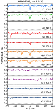
Figure 11: Stacked velocity plot for the $z=3.2430$ system towards J0100-2708. Solid histograms show the normalized flux as a function of velocity offset from the nominal redshift. The thin solid line at the bottom of each panel marks the 1$\sigma$ flux uncertainty. Solid shading marks the intervals over which equivalent widths were measured. Hatched shading (in this and other figures) denotes lines that are either blended with an unrelated absorber or contaminated by strong telluric residuals.

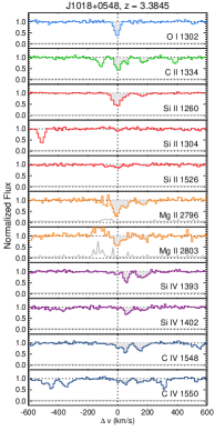
Figure 12: Stacked velocity plot for the $z=3.3845$ system towards J1018+0548. Lines and shading are as described in Figure 12.

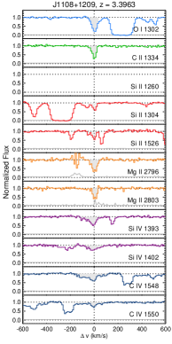
Figure 13: Stacked velocity plot for the $z=3.3963$ system towards J1108+1209. Lines and shading are as described in Figure 12.

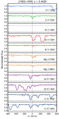
Figure 14: Stacked velocity plot for the $z=3.4423$ system towards J1552+1005. Lines and shading are as described in Figure 12.

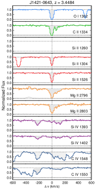
Figure 15: Stacked velocity plot for the $z=3.4484$ system towards J1421-0643. Lines and shading are as described in Figure 12.

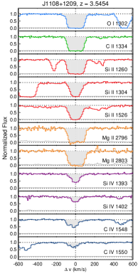
Figure 16: Stacked velocity plot for the $z=3.5454$ system towards J1108+1209. Lines and shading are as described in Figure 12.

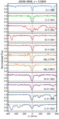
Figure 17: Stacked velocity plot for the $z=3.5804$ system towards J0056-2808. Lines and shading are as described in Figure 12.

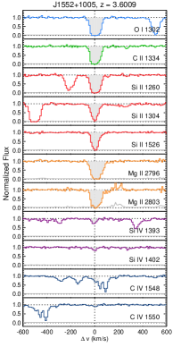
Figure 18: Stacked velocity plot for the $z=3.6009$ system towards J1552+1005. Lines and shading are as described in Figure 12.

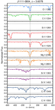
Figure 19: Stacked velocity plot for the $z=3.6078$ system towards J1111-0804. Lines and shading are as described in Figure 12.

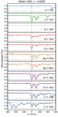
Figure 20: Stacked velocity plot for the $z=3.6287$ system towards J0042-1020. Lines and shading are as described in Figure 12. See notes on this system in Appendix B.

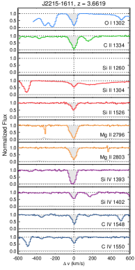
Figure 21: Stacked velocity plot for the $z=3.6619$ system towards J2215-1611. Lines and shading are as described in Figure 12.

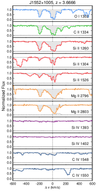
Figure 22: Stacked velocity plot for the $z=3.6666$ system towards J1552+1005. Lines and shading are as described in Figure 12.

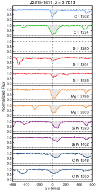
Figure 23: Stacked velocity plot for the $z=3.7013$ system towards J2215-1611. Lines and shading are as described in Figure 12. See notes on this system in Appendix B.

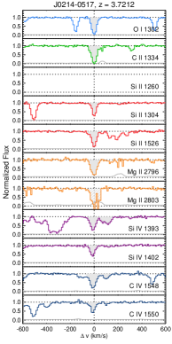
Figure 24: Stacked velocity plot for the $z=3.7212$ system towards J0214-0517. Lines and shading are as described in Figure 12.

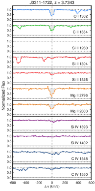
Figure 25: Stacked velocity plot for the $z=3.7343$ system towards J0311-1722. Lines and shading are as described in Figure 12.

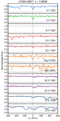
Figure 26: Stacked velocity plot for the $z=3.8039$ system towards J1032+0927. Lines and shading are as described in Figure 12. The grey histogram in the O I $\lambda$1302 panel is the deblended flux. See notes on this system in Appendix B.

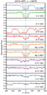
Figure 27: Stacked velocity plot for the $z=3.8079$ system towards J0415-4357. Lines and shading are as described in Figure 12. The grey histogram in the O I $\lambda$1302 panel is the deblended flux. See notes on this system in Appendix B.

Figure 28: Stacked velocity plot for the $z=3.9007$ system towards J0747+2739. Lines and shading are as described in Figure 12.

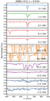
Figure 29: Stacked velocity plot for the $z=3.9124$ system towards J0959+1312. Lines and shading are as described in Figure 12.

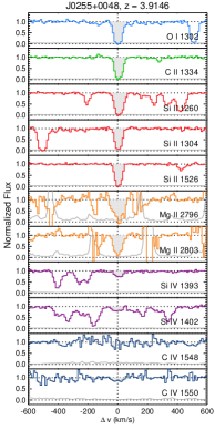
Figure 30: Stacked velocity plot for the $z=3.9146$ system towards J0255+0048. Lines and shading are as described in Figure 12.

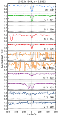
Figure 31: Stacked velocity plot for the $z=3.9362$ system towards J0132+1341. Lines and shading are as described in Figure 12.

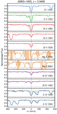
Figure 32: Stacked velocity plot for the $z=3.9465$ system towards J0800+1920. Lines and shading are as described in Figure 12.

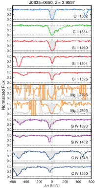
Figure 33: Stacked velocity plot for the $z=3.9557$ system towards J0835+0650. Lines and shading are as described in Figure 12. See notes on this system in Appendix B.

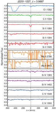
Figure 34: Stacked velocity plot for the $z=3.9887$ system towards J2251-1227. Lines and shading are as described in Figure 12.

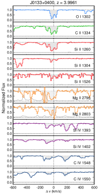
Figure 35: Stacked velocity plot for the $z=3.9961$ system towards J0133+0400. Lines and shading are as described in Figure 12.

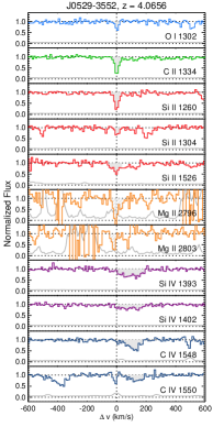
Figure 36: Stacked velocity plot for the $z=4.0656$ system towards J0529-3552. Lines and shading are as described in Figure 12.

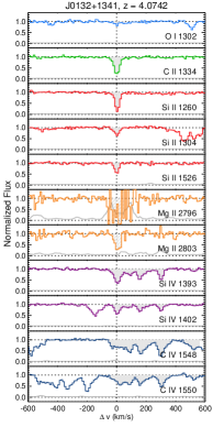
Figure 37: Stacked velocity plot for the $z=4.0742$ system towards J0132+1341. Lines and shading are as described in Figure 12. See notes on this system in Appendix B.

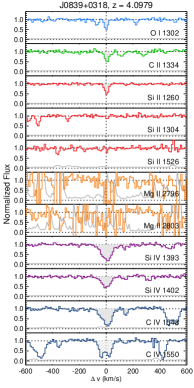
Figure 38: Stacked velocity plot for the $z=4.0979$ system towards J0839+0318. Lines and shading are as described in Figure 12.

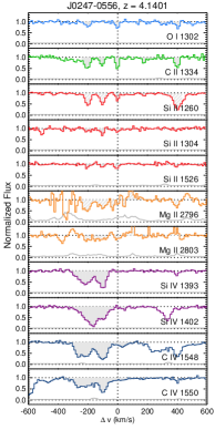
Figure 39: Stacked velocity plot for the $z=4.1401$ system towards J0247-0556. Lines and shading are as described in Figure 12. See notes on this system in Appendix B.

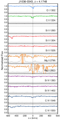
Figure 40: Stacked velocity plot for the $z=4.1748$ system towards J1036-0343. Lines and shading are as described in Figure 12.

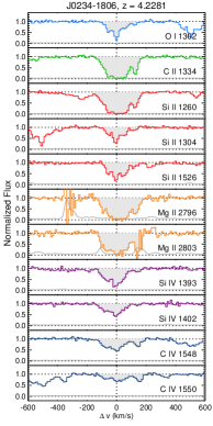
Figure 41: Stacked velocity plot for the $z=4.2281$ system towards J0234-1806. Lines and shading are as described in Figure 12.

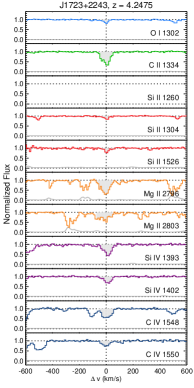
Figure 42: Stacked velocity plot for the $z=4.2475$ system towards J1723+2243. Lines and shading are as described in Figure 12.

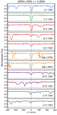
Figure 43: Stacked velocity plot for the $z=4.2524$ system towards J0034+1639. Lines and shading are as described in Figure 12.

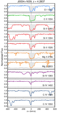
Figure 44: Stacked velocity plot for the $z=4.2837$ system towards J0034+1639. Lines and shading are as described in Figure 12.

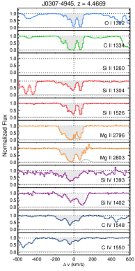
Figure 45: Stacked velocity plot for the $z=4.4669$ system towards J0307-4945. Lines and shading are as described in Figure 12.

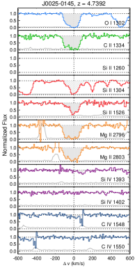
Figure 46: Stacked velocity plot for the $z=4.7392$ system towards J0025-0145. Lines and shading are as described in Figure 12.

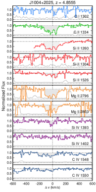
Figure 47: Stacked velocity plot for the $z=4.8555$ system towards J1004+2025. Lines and shading are as described in Figure 12. See notes on this system in Appendix B.

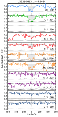
Figure 48: Stacked velocity plot for the $z=4.9464$ system towards J2325-0553. Lines and shading are as described in Figure 12.

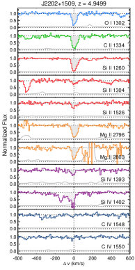
Figure 49: Stacked velocity plot for the $z=4.9499$ system towards J2202+1509. Lines and shading are as described in Figure 12.

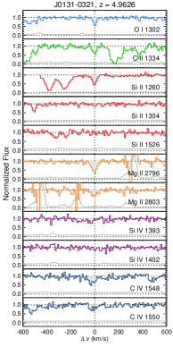
Figure 50: Stacked velocity plot for the $z=4.9626$ system towards J0131-0321. Lines and shading are as described in Figure 12.

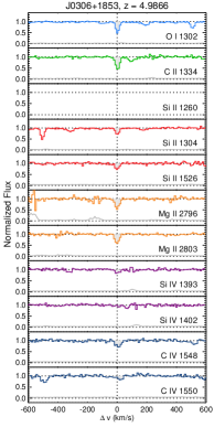
Figure 51: Stacked velocity plot for the $z=4.9866$ system towards J0306+1853. Lines and shading are as described in Figure 12.

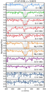
Figure 52: Stacked velocity plot for the $z=5.0615$ system towards J1147-0109. Lines and shading are as described in Figure 12. See notes on this system in Appendix B.

Figure 53: Stacked velocity plot for the $z=5.1052$ system towards J0812+0440. Lines and shading are as described in Figure 12.

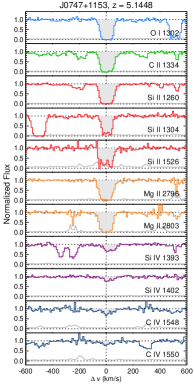
Figure 54: Stacked velocity plot for the $z=5.1448$ system towards J0747+1153. Lines and shading are as described in Figure 12.

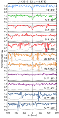
Figure 55: Stacked velocity plot for the $z=5.1783$ system towards J1436+2132. Lines and shading are as described in Figure 12.

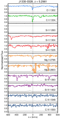
Figure 56: Stacked velocity plot for the $z=5.2961$ system towards J1335-0328. Lines and shading are as described in Figure 12. The grey histogram in the O I $\lambda$1302 panel is the deblended flux. See notes on this system in Appendix B.

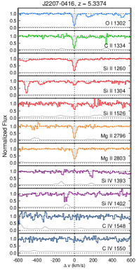
Figure 57: Stacked velocity plot for the $z=5.3374$ system towards J2207-0416. Lines and shading are as described in Figure 12.

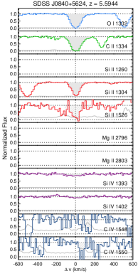
Figure 58: Stacked velocity plot for the $z=5.5944$ system towards SDSS J0840+5624. Lines and shading are as described in Figure 12.

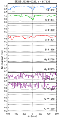
Figure 59: Stacked velocity plot for the $z=5.7533$ system towards SDSS J2315-0023. Lines and shading are as described in Figure 12.

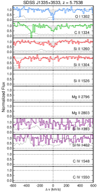
Figure 60: Stacked velocity plot for the $z=5.7538$ system towards SDSS J1335+3533. Lines and shading are as described in Figure 12.

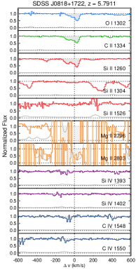
Figure 61: Stacked velocity plot for the $z=5.7911$ system towards SDSS J0818+1722. Lines and shading are as described in Figure 12.

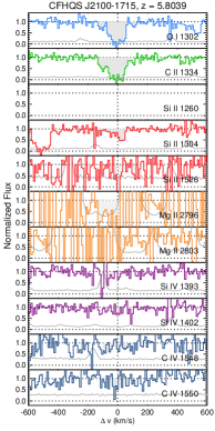
Figure 62: Stacked velocity plot for the $z=5.8039$ system towards CFHQS J2100-1715. Lines and shading are as described in Figure 12.

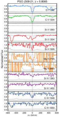
Figure 63: Stacked velocity plot for the $z=5.8085$ system towards PSO J308-21. Lines and shading are as described in Figure 12.

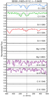
Figure 64: Stacked velocity plot for the $z=5.8425$ system towards SDSS J1623+3112. Lines and shading are as described in Figure 12.

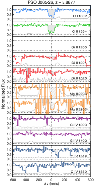
Figure 65: Stacked velocity plot for the $z=5.8677$ system towards PSO J065-26. Lines and shading are as described in Figure 12.

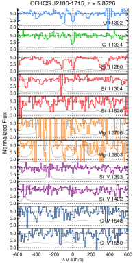
Figure 66: Stacked velocity plot for the $z=5.8726$ system towards CFHQS J2100-1715. Lines and shading are as described in Figure 12.

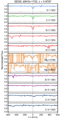
Figure 67: Stacked velocity plot for the $z=5.8767$ system towards SDSS J0818+1722. Lines and shading are as described in Figure 12.

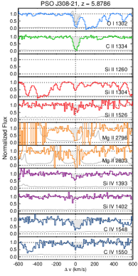
Figure 68: Stacked velocity plot for the $z=5.8786$ system towards PSO J308-21. Lines and shading are as described in Figure 12. The grey histogram in the O I $\lambda$1302 panel is the deblended flux. See notes on this system in Appendix B.

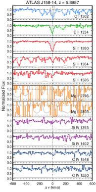
Figure 69: Stacked velocity plot for the $z=5.8987$ system towards ATLAS J158-14. Lines and shading are as described in Figure 12. The grey histogram in the O I $\lambda$1302 panel is the deblended flux. See notes on this system in Appendix B.

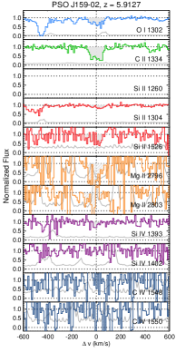
Figure 70: Stacked velocity plot for the $z=5.9127$ system towards PSO J159-02. Lines and shading are as described in Figure 12.

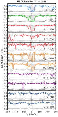
Figure 71: Stacked velocity plot for the $z=5.9366$ system towards PSO J056-16. Lines and shading are as described in Figure 12.

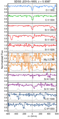
Figure 72: Stacked velocity plot for the $z=5.9387$ system towards SDSS J2310+1855. Lines and shading are as described in Figure 12.

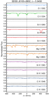
Figure 73: Stacked velocity plot for the $z=5.9450$ system towards SDSS J0100+2802. Lines and shading are as described in Figure 12. The grey histogram in the C II $\lambda$1334 panel is the deblended flux. See notes on this system in Appendix B.

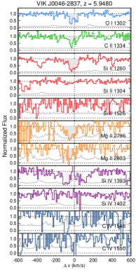
Figure 74: Stacked velocity plot for the $z=5.9480$ system towards VIK J0046-2837. Lines and shading are as described in Figure 12.

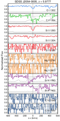
Figure 75: Stacked velocity plot for the $z=5.9777$ system towards SDSS J2054-0005. Lines and shading are as described in Figure 12.

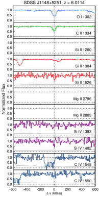
Figure 76: Stacked velocity plot for the $z=6.0114$ system towards SDSS J1148+5251. Lines and shading are as described in Figure 12. See notes on this system in Appendix B.

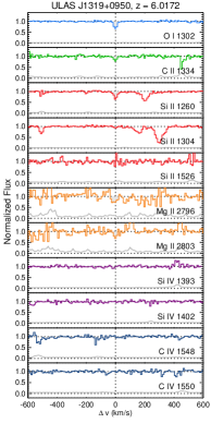
Figure 77: Stacked velocity plot for the $z=6.0172$ system towards ULAS J1319+0950. Lines and shading are as described in Figure 12.

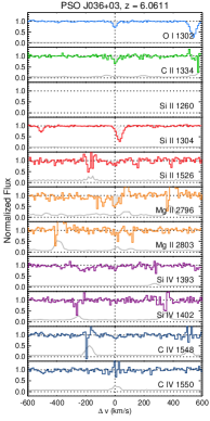
Figure 78: Stacked velocity plot for the $z=6.0611$ system towards PSO J036+03. Lines and shading are as described in Figure 12.

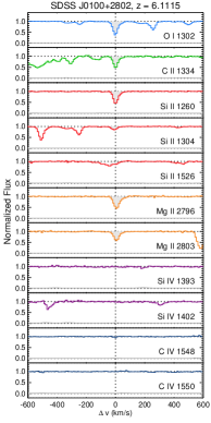
Figure 79: Stacked velocity plot for the $z=6.1115$ system towards SDSS J0100+2802. Lines and shading are as described in Figure 12.

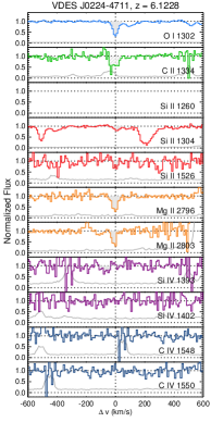
Figure 80: Stacked velocity plot for the $z=6.1228$ system towards VDES J0224-4711. Lines and shading are as described in Figure 12.

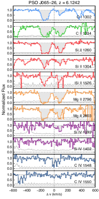
Figure 81: Stacked velocity plot for the $z=6.1242$ system towards PSO J065-26. Lines and shading are as described in Figure 12. See notes on this system in Appendix B.

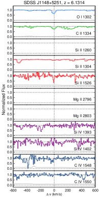
Figure 82: Stacked velocity plot for the $z=6.1314$ system towards SDSS J1148+5251. Lines and shading are as described in Figure 12. See notes on this system in Appendix B.

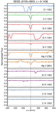
Figure 83: Stacked velocity plot for the $z=6.1436$ system towards SDSS J0100+2802. Lines and shading are as described in Figure 12.

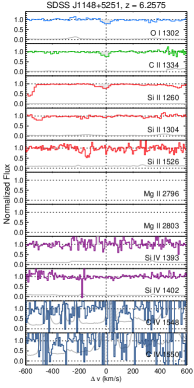
Figure 84: Stacked velocity plot for the $z=6.2575$ system towards SDSS J1148+5251. Lines and shading are as described in Figure 12. See notes on this system in Appendix B.

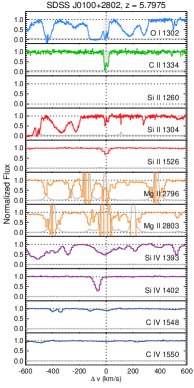
Figure 85: Stacked velocity plot for the $z=5.7975$ system towards SDSS J0100+2802. Lines and shading are as described in Figure 12. The data for O I $\lambda$1302, C II $\lambda$1334, and Si II $\lambda$1304 are from HIRES. This system falls outside of the nominal survey range for this QSO and is not included in our statistical sample.

References

- Asplund et al. (2009) Asplund, M., Grevesse, N., Sauval, A. J., & Scott, P. 2009, ARAA, 47, 481
- Bahcall & Peebles (1969) Bahcall, J. N., & Peebles, P. J. E. 1969, ApJ, 156, L7
- Bañados et al. (2017) Bañados, E., Venemans, B. P., Mazzucchelli, C., et al. 2017, eprint arXiv, 1712, arXiv:1712.01860
- Becker et al. (2015) Becker, G. D., Bolton, J. S., Madau, P., et al. 2015, MNRAS, 447, 3402
- Becker et al. (2009) Becker, G. D., Rauch, M., & Sargent, W. L. W. 2009, ApJ, 698, 1010
- Becker et al. (2011) Becker, G. D., Sargent, W. L. W., & Rauch, M. 2011, ApJ, 735, 93
- Becker et al. (2012) Becker, G. D., Sargent, W. L. W., Rauch, M., & Carswell, R. F. 2012, ApJ, 744, 91
- Becker et al. (2006) Becker, G. D., Sargent, W. L. W., Rauch, M., & Simcoe, R. A. 2006, ApJ, 640, 69
- Berg et al. (2016) Berg, T. a. M., Ellison, S. L., Sánchez-Ramírez, R., et al. 2016, MNRAS, 463, 3021
- Boera et al. (2019) Boera, E., Becker, G. D., Bolton, J. S., & Nasir, F. 2019, ApJ, 872, 101
- Bosman et al. (2017) Bosman, S. E. I., Becker, G. D., Haehnelt, M. G., et al. 2017, MNRAS, 470, 1919
- Bosman et al. (2018) Bosman, S. E. I., Fan, X., Jiang, L., et al. 2018, MNRAS, 479, 1055
- Bowler et al. (2014) Bowler, R. A. A., Hewett, P. C., Allen, J. T., & Ferland, G. J. 2014, MNRAS, 445, 359
- Calverley et al. (2011) Calverley, A. P., Becker, G. D., Haehnelt, M. G., & Bolton, J. S. 2011, MNRAS, 412, 2543
- Chambaud et al. (1980) Chambaud, G., Levy, B., Launay, J. M., et al. 1980, JPhB, 13, 4205
- Chen et al. (2017) Chen, S.-F. S., Simcoe, R. A., Torrey, P., et al. 2017, ApJ, 850, 188
- Codoreanu et al. (2017) Codoreanu, A., Ryan-Weber, E. V., Crighton, N. H. M., et al. 2017, MNRAS, 472, 1023
- Codoreanu et al. (2018) Codoreanu, A., Ryan-Weber, E. V., García, L. Á., et al. 2018, MNRAS, 481, 4940
- Cooke et al. (2011) Cooke, R., Pettini, M., Steidel, C. C., & Rudie, G. C. 2011, MNRAS, 417, 1534
- Cooper et al. (2019) Cooper, T. J., Simcoe, R. A., Cooksey, K. L., et al. 2019, arXiv:1901.05980
- Crociani et al. (2011) Crociani, D., Mesinger, A., Moscardini, L., & Furlanetto, S. 2011, MNRAS, 411, 289
- D’Aloisio et al. (2018) D’Aloisio, A., McQuinn, M., Davies, F. B., & Furlanetto, S. R. 2018, MNRAS, 473, 560
- Davies & Furlanetto (2016) Davies, F. B., & Furlanetto, S. R. 2016, MNRAS, 460, 1328
- Davies et al. (2018) Davies, F. B., Hennawi, J. F., Eilers, A.-C., & Lukić, Z. 2018, ApJ, 855, 106
- Dessauges-Zavadsky et al. (2003) Dessauges-Zavadsky, M., Péroux, C., Kim, T.-S., D’Odorico, S., & McMahon, R. G. 2003, MNRAS, 345, 447
- D’Odorico et al. (2013) D’Odorico, V., Cupani, G., Cristiani, S., et al. 2013, MNRAS, 435, 1198
- D’Odorico et al. (2018) D’Odorico, V., Feruglio, C., Ferrara, A., et al. 2018, ApJ, 863, L29
- Doughty et al. (2018) Doughty, C., Finlator, K., Oppenheimer, B. D., Davé, R., & Zackrisson, E. 2018, MNRAS, 475, 4717
- Eilers et al. (2018) Eilers, A.-C., Davies, F. B., & Hennawi, J. F. 2018, ApJ, 864, 53
- Ellison et al. (2010) Ellison, S. L., Prochaska, J. X., Lopez, S., et al. 2010, MNRAS, 406, 1435
- Ellison et al. (2011) Ellison, S. L., Prochaska, J. X., & Mendel, J. T. 2011, MNRAS, 412, 448
- Fan et al. (2006) Fan, X., Strauss, M. A., Becker, R. H., et al. 2006, AJ, 132, 117
- Fernandez & Shull (2011) Fernandez, E. R., & Shull, J. M. 2011, ApJ, 731, 20
- Finlator et al. (2018) Finlator, K., Keating, L., Oppenheimer, B. D., Davé, R., & Zackrisson, E. 2018, MNRAS, 480, 2628
- Finlator et al. (2013) Finlator, K., Muñoz, J. A., Oppenheimer, B. D., et al. 2013, MNRAS, 436, 1818
- Finlator et al. (2016) Finlator, K., Oppenheimer, B. D., Davé, R., et al. 2016, MNRAS, 459, 2299
- Finlator et al. (2015) Finlator, K., Thompson, R., Huang, S., et al. 2015, MNRAS, 447, 2526
- Fox et al. (2007) Fox, A. J., Ledoux, C., Petitjean, P., & Srianand, R. 2007, A&A, 473, 791
- Furlanetto & Loeb (2003) Furlanetto, S. R., & Loeb, A. 2003, ApJ, 588, 18
- García et al. (2017) García, L. A., Tescari, E., Ryan-Weber, E. V., & Wyithe, J. S. B. 2017, MNRAS, 470, 2494
- Haardt & Madau (2012) Haardt, F., & Madau, P. 2012, ApJ, 746, 125
- Hoag et al. (2019) Hoag, A., Bradač, M., Huang, K., et al. 2019, ApJ, 878, 12
- Horne (1986) Horne, K. 1986, PASP, 98, 609
- Jones et al. (2013) Jones, T., Ellis, R. S., Schenker, M. A., & Stark, D. P. 2013, arXiv:1304.7015
- Keating et al. (2014) Keating, L. C., Haehnelt, M. G., Becker, G. D., & Bolton, J. S. 2014, MNRAS, 438, 1820
- Keating et al. (2019) Keating, L. C., Weinberger, L. H., Kulkarni, G., et al. 2019, arXiv:1905.12640
- Kelson (2003) Kelson, D. D. 2003, PASP, 115, 688
- Kuhlen & Faucher-Giguère (2012) Kuhlen, M., & Faucher-Giguère, C.-A. 2012, MNRAS, 423, 862
- Kulkarni et al. (2019) Kulkarni, G., Keating, L. C., Haehnelt, M. G., et al. 2019, MNRAS, 485, L24
- Lopez et al. (2016) Lopez, S., D’Odorico, V., Ellison, S. L., et al. 2016, A&A, 594, A91
- Ma et al. (2016) Ma, X., Hopkins, P. F., Kasen, D., et al. 2016, MNRAS, 459, 3614
- Mason et al. (2019) Mason, C. A., Fontana, A., Treu, T., et al. 2019, MNRAS, 485, 3947
- Matejek & Simcoe (2012) Matejek, M. S., & Simcoe, R. A. 2012, ApJ, 761, 112
- Mathes et al. (2017) Mathes, N. L., Churchill, C. W., & Murphy, M. T. 2017, arXiv:1701.05624
- McQuinn et al. (2011) McQuinn, M., Oh, S. P., & Faucher-Giguère, C.-A. 2011, ApJ, 743, 82
- Ménard et al. (2011) Ménard, B., Wild, V., Nestor, D., et al. 2011, MNRAS, 417, 801
- Mesinger & Furlanetto (2009) Mesinger, A., & Furlanetto, S. 2009, MNRAS, 400, 1461
- Meyer et al. (2019) Meyer, R. A., Bosman, S. E. I., Kakiichi, K., & Ellis, R. S. 2019, MNRAS, 483, 19
- Milne (1926) Milne, E. A. 1926, MNRAS, 86, 459
- Nestor et al. (2008) Nestor, D., Hamann, F., & Rodriguez Hidalgo, P. 2008, MNRAS, 386, 2055
- Noll et al. (2012) Noll, S., Kausch, W., Barden, M., et al. 2012, A&A, 543, A92
- Oh (2002) Oh, S. P. 2002, MNRAS, 336, 1021
- Oppenheimer & Davé (2006) Oppenheimer, B. D., & Davé, R. 2006, MNRAS, 373, 1265
- Oppenheimer et al. (2009) Oppenheimer, B. D., Davé, R., & Finlator, K. 2009, MNRAS, 396, 729
- Péroux et al. (2007) Péroux, C., Dessauges-Zavadsky, M., D’Odorico, S., Kim, T.-S., & McMahon, R. G. 2007, MNRAS, 382, 177
- Perrotta et al. (2016) Perrotta, S., D’Odorico, V., Prochaska, J. X., et al. 2016, MNRAS, 462, 3285
- Rafelski et al. (2014) Rafelski, M., Neeleman, M., Fumagalli, M., Wolfe, A. M., & Prochaska, J. X. 2014, ApJl, 782, L29
- Rafelski et al. (2012) Rafelski, M., Wolfe, A. M., Prochaska, J. X., Neeleman, M., & Mendez, A. J. 2012, ApJ, 755, 89
- Rauch et al. (2008) Rauch, M., Haehnelt, M., Bunker, A., et al. 2008, ApJ, 681, 856
- Ryan-Weber et al. (2009) Ryan-Weber, E. V., Pettini, M., Madau, P., & Zych, B. J. 2009, MNRAS, 395, 1476
- Sánchez-Ramírez et al. (2016) Sánchez-Ramírez, R., Ellison, S. L., Prochaska, J. X., et al. 2016, MNRAS, 456, 4488
- Scargle (1973) Scargle, J. D. 1973, ApJ, 179, 705
- Sheinis et al. (2002) Sheinis, A. I., Bolte, M., Epps, H. W., et al. 2002, PASP, 114, 851
- Simcoe (2011) Simcoe, R. A. 2011, ApJ, 738, 159
- Simcoe et al. (2011) Simcoe, R. A., Cooksey, K. L., Matejek, M., et al. 2011, ApJ, 743, 21
- Stancil et al. (1999) Stancil, P. C., Schultz, D. R., Kimura, M., et al. 1999, A&AS, 140, 225
- Steidel et al. (2011) Steidel, C. C., Bogosavljević, M., Shapley, A. E., et al. 2011, ApJ, 736, 160
- Steidel et al. (2018) —. 2018, ApJ, 869, 123
- Tumlinson et al. (2017) Tumlinson, J., Peeples, M. S., & Werk, J. K. 2017, ARAA, 55, 389
- Vernet et al. (2011) Vernet, J., Dekker, H., D’Odorico, S., et al. 2011, A&A, 536, A105
- Vogt et al. (1994) Vogt, S. S., Allen, S. L., Bigelow, B. C., et al. 1994, Proc. SPIE, 2198, 362
- Weymann et al. (1979) Weymann, R. J., Williams, R. E., Peterson, B. M., & Turnshek, D. A. 1979, ApJ, 234, 33
- Wild et al. (2008) Wild, V., Kauffmann, G., White, S., et al. 2008, MNRAS, 388, 227
- Wisotzki et al. (2018) Wisotzki, L., Bacon, R., Brinchmann, J., et al. 2018, Nature, 562, 229
- Wolfe et al. (2005) Wolfe, A. M., Gawiser, E., & Prochaska, J. X. 2005, ARAA, 43, 861
- Wu et al. (2015) Wu, X.-B., Wang, F., Fan, X., et al. 2015, Nature, 518, 512
- Wyithe & Bolton (2011) Wyithe, J. S. B., & Bolton, J. S. 2011, MNRAS, 412, 1926