A Comparison of Flare Forecasting Methods. III. Systematic Behaviors of Operational Solar Flare Forecasting Systems

Abstract

A workshop was recently held at Nagoya University (31 October – 02 November 2017), sponsored by the Center for International Collaborative Research, at the Institute for Space-Earth Environmental Research, Nagoya University, Japan, to quantitatively compare the performance of today’s operational solar flare forecasting facilities. Building upon Paper I of this series (Barnes et al., 2016), in Paper II (Leka et al., 2019) we described the participating methods for this latest comparison effort, the evaluation methodology, and presented quantitative comparisons. In this paper we focus on the behavior and performance of the methods when evaluated in the context of broad implementation differences. Acknowledging the short testing interval available and the small number of methods available, we do find that forecast performance: 1) appears to improve by including persistence or prior flare activity, region evolution, and a human “forecaster in the loop”; 2) is hurt by restricting data to disk-center observations; 3) may benefit from long-term statistics, but mostly when then combined with modern data sources and statistical approaches. These trends are arguably weak and must be viewed with numerous caveats, as discussed both here and in Paper II. Following this present work, we present in Paper IV a novel analysis method to evaluate temporal patterns of forecasting errors of both types (i.e., misses and false alarms; Park et al., 2019). Hence, most importantly, with this series of papers we demonstrate the techniques for facilitating comparisons in the interest of establishing performance-positive methodologies.

1 Introduction

In 2009, the first in a series of workshops was held to compare and evaluate solar flare forecasting methods; the results and comparison methodologies were presented in Barnes et al. (2016, ; Paper I) and have informed numerous works. In Leka et al. (2019, ‘Paper II’), the initial results from the most recent “head-to-head” comparison of operational flare-forecasting methods are presented. The comparison is the output of a 3-day workshop held at the Institute for Space-Earth Environmental Research (ISEE) at Nagoya University over 31 October – 02 November 2017, and was sponsored by the ISEE Center for International Collaborative Research. In that paper, the methodology was presented: the agreed-upon testing interval, event definitions, and evaluation metrics were described. Specifically, daily operational full-disk forecasts from a variety of facilities were gathered for 2016–2017, specifically for two event definitions: C1.0+/0/24 and M1.0+/0/24 which indicate minimum-threshold for an event, the latency between forecast issuance and validity period start, and the validity period itself. The results demonstrated broad performance similarities across numerous metrics for the majority of methods. The “winner” depended on event definition and metric used. However, within the estimated uncertainties, a more appropriate description is that a number of methods consistently scored above the “no skill” level.

Simply comparing the performance is of limited use if there is no investigation into “why”, from which we may derive how improvements could be made. The question we investigate here is “are there certain aspects, certain approaches or methodologies implemented by the different methods that influence the performance in a discernible, distinguishable way?”

The participating facilities and methods (and their monikers and published references, where available) are listed in Table 1 of Paper II, with details that are not available by published literature are briefly described in that paper’s Appendix; an abbreviated version of that table is reproduced here in Appendix A. The submitted forecasts are also available. We take the descriptions further here, into the details of implementation that the workshop group hypothesized may factor into performance.

2 Methodology

The approach here is to identify general categories by which the methods could be grouped, and then examine whether there are systematic performance differences according to those categories across a variety of quantitative evaluation metrics. As such, “the devil is in the details” and in most cases there was significant additional information needed than what is readily available in the literature (see also Paper II, Appendix A).

The participants wanted to determine whether implementation differences could make a significant difference to the forecast performance. In Barnes et al. (2016), this question was briefly investigated: we examined the impact of subtle differences in how a commonly-used analysis quantity, the total magnetic flux, was calculated (e.g., any noise threshold used, the specific de-projection method employed, if any). could in fact significantly impact the evaluation results. For operational systems, for example, one can imagine that restricting the relevant data analysis to near-disk-center data will result in a systematic underperformance in full-disk forecasts due to missing regions. Were there any such situations? And what was the magnitude of such an impact?

Given the complexity of operational forecasting facilities, we asked “at what other steps in the process were there multiple options available?”, and “is it possible to determine the impact of such options on performance outcomes?” We identified four broad stages at which differences arose: 1) the data used and how they are treated; 2) the specifics of training the method; 3) the specifics of producing the forecast; 4) the actual issuance of the forecast itself.

All methods were requested to comment on specific questions regarding particular aspects that were known to vary between methods which the group felt may impact performance. The topics and the responses are summarized in Tables 1–4. Some methods have multiple options for producing forecasts, and those are delineated within the table. Acronyms are used for brevity in the tables and figures and some of the discussion, but are expanded upon in Appendix B.

This approach will not capture all possible subtleties. For example, DAFFS and DAFFS-G may use a measure of prior flare activity with some event definitions but not others, and this may change upon periodic re-training. As another example, many methods use NOAA active-region designations, others use HMI “active region patches” (HARPs; Hoeksema et al., 2014)) that may or may not agree in their entirety with the NOAA designations, while other methods use various algorithms to independently determine solar magnetic regions. Some of those methods have the goal of matching the NOAA designations, but some algorithms perform region identification explicitly without that goal (such as the HMI algorithm). For the tests here, the region-assigned probabilities for all regions were combined (generally by the methods themselves) to produce full-disk probabilities, but questions linger as to how differences in region determination impacts the training (upon which forecasts are then based). Still, we attempt to answer what is answerable, or at least demonstrate an appropriate methodology for doing so.

The metrics used here are the same as in Paper II (Leka et al., 2019), representing a mix of scores based on probabilistic and dichotomous forecasts. For the latter, a single probability threshold $P_{\rm th}=0.5$ is applied for the evaluation, and all other considerations regarding the metric calculations discussed in Paper II are applied here. Essentially the individual scores have not changed from those presented in Paper II, but what has changed is that each method is assigned membership to a particular group (see Section 2.1) and the resulting scores from within each group are presented together. Instead of presenting the scores for each method individually, we emphasize variation between categories by showing “box & whisker” plots.

For the analysis here, two Paper II methods are generally excluded. The first is the 120-day prior climatology forecast, an “unskilled” forecast that can be constructed at the time of forecast issuance. It was presented in Paper II (following Sharpe & Murray, 2017) for evaluation across the metrics, and used as the reference forecast for two skill scores in order to specifically measure skill beyond a no-skill forecast method. In this analysis it is still used as a reference forecast for the ApSS_clim and MSESS_clim metrics, however it is not presented on its own for evaluation (as was done in Paper II), because we focus here on methods that hopefully bring added value beyond an unskilled method.

The second method excluded from the quantitative analysis is the NJIT method. As discussed in Paper II, the NJIT method represents a research project that was never fully transitioned to operations, and as such suffers in numerous metrics from missing forecasts; it is a consistent outlier. Again, with a focus on operational methods, for this analysis we omit the NJIT forecasts when computing the metrics (although we include its details in the Tables for future reference).

Table 1: Devil-is-in-the-Details Summary
Forecast Data Sources and Treatment: What are primary, backup data sources? Is there a protocol for bad / missing data? If using $B_{\rm los}$, are any corrections used? Are there limits on the data? Is there any special treatment of the data?

Method	Response
A-EFFORT	HMI NRT FD $B_{\rm los}$ data, $B_{r}^{los}=B_{\rm los}/\cos(\theta)$ & heliographic-plane projection, HMI-to-MDI emulation, NOAA SRS AR assignments; missing data protocol: prior forecast does not refresh
AMOS	NOAA-reported flare events and NOAA SRS AR reports (2 days’ worth); missing data protocol: prior forecast does not refresh.
ASAP	HMI NRT FD $B_{\rm los}$ & Continuum; No protocol for missing data; not using $B_{\rm los}$ quantitatively (region identification only).
ASSA	HMI NRT FD $B_{\rm los}$ & Continuum; No protocol for missing data. No correction to $B_{\rm los}$ but sunspots located $>80^{\circ}$ from the limb are excluded.
BOM	NOAA/SWPC SRS, USAF SOON reports, HMI NRT $B_{\rm los}$ rebinned by x4; replaced by definitive data after a few days (for future training); bad/missing data protocol: reverts to forecasts by region classification / area / flare rates.
DAFFS, DAFFS-G	HMI NRT $\vec{\bf B}$ and NRT HARP designations, NOAA NRT GOES-based X-ray event lists (DAFFS), GONG $B_{\rm los}$ + GOES for DAFFS-G, used when HMI data not available; if neither HMI or GONG are available, GOES X-ray events used with NOAA AR designations; training-interval climatology as last resort. $B_{\rm los}$ data: uses $B_{r}^{\rm pot}$ estimate (Leka et al., 2017).
MAG4	HMI NRT FD $B_{\rm los}$ (GONG manually as backup; not employed here), $\vec{\bf B}$ data, NOAA SRS AR assignments, NOAA-reported flare events; LMSAL/SolarSoft events as back-up. Use last good data up to 60-96 minutes delay, else repeat last forecast. Prior flaring (MAG4*F) set to null if data are unavailable. No correction to $B_{\rm los}$. Limits imposed on training data (see Table 3).
MCSTAT, MCEVOL	NOAA flare event and SRS reports (Zpc classes); missing SRS report protocol: 0% forecast.
MOSWOC	HMI images, SWPC AR numbers. SDO data used qualitatively.
NICT	NOAA SRS & GOES, HMI imaging data, HMI SHARP parameters, AIA imaging data, ground-based data as backup. SDO data used qualitatively.
NJIT	NOAA SRS & HMI $B_{\rm los},\cos(\theta)$ correction; helicity is not computed (and no forecast is issued) if NRT data are not downloaded or available in the NJIT flare forecasting system (for any reason).
NOAA	NOAA & USAF imagery, flare reports, radio data; any & all imagery, primarily NOAA-assured operational sources (including GOES, GONG assets), other as needed/available. SDO data used qualitatively. No protocol for outtages beyond “any and all” data used.
SIDC	NOAA SRS and Catania Obs; GOES flare history (PROBA2/LYRA as backup); SDO/HMI magnetogram and continuum movies, EUV images (SDO/AIA, PROBA2/SWAP as backup, and STEREO/EUVI), especially for limb-ward regions.

Table 2: Devil-is-in-the-Details Summary (cont’d)
Full-Disk Forecast Production: How are active regions identified? How are full-disk forecasts constructed? Is there any explicit forecasting for behind-the-limb events?

Method	Response
A-EFFORT	Regions IDd via ARIA (LaBonte et al., 2007; Georgoulis et al., 2008); FD forecasts via region probabilities. No behind-limb forecasts
AMOS	Regions ID’d by NOAA/SRS files; FD forecasts via region probabilities.
ASAP	ML code to identify / classify sunspot regions using intensity and $B_{\rm los}$ images. No full-disk prediction (region only).
ASSA	In-house automatic ID and classification of McIntosh & Mt Wilson Classes. Probabilities from classification, Poisson statistics. FD forecasts via region probabilities.
BOM	Automatic recognition of ARs by magnetogram flux thresholds, NOAA/SRS and USAF/SOON as backup. FD forecasts via region probabilities. No explicit behind-the-limb forecasts or multi-day forecasts, although very-near limb regions assigned region-flaring climatology.
DAFFS, DAFFS-G	HARPs (HMI, for DAFFS) or NOAA NRT region-based areas (GARPS, for GONG for DAFFS-G) ID’d, extracted. FD forecasts via region probabilities. No explicit behind-the-limb forecasts beyond multi-day forecasts.
MAG4	NOAA/SRS ARs, FD forecasts via region probabilities. No explicit behind-the-limb forecasts beyond multi-day forecasts.
MCSTAT, MCEVOL	NOAA/SRS ARs reports
MOSWOC	NOAA/SRS ARs plus additional regions ID’d and assigned Mt Wilson & McIntosh classes if needed, updated 4x/day. FD forecasts via region probabilities. No explicit behind-the-limb forecasts beyond multi-day forecasts
NICT	NOAA/SRS information is used internally, but FD forecasts only are issued.
NJIT	NOAA/SRS used for AR identification, FD forecasts via region probabilities.
NOAA	NOAA/SWPC produces region identification and classification, disseminates. FD forecasts via region probabilities. Forecasts include probabilities for behind-the-limb activity.
SIDC	Catania Region identification & NOAA/SRS for region probabilities then FD forecasts via region probabilities, human modified (e.g, for new or behind-the-limb regions)

Table 3: Devil-is-in-the-Details Summary (cont’d)
Training: What data are used, what is optimized / produced? Are balanced training sets imposed or is class (event / no-event) imbalance accomodated? What interval is used in general / for this test (if different)? Is there a protocol for training for behind-the-limb or unassigned events?

Method	Response
A-EFFORT	Forecasts curves constructed, no further optimization. 80% of calendar days of archive data, contiguous or random select. 3-hr forecast cadence for first 12 months of servce; balancing in training to a 4:1 (time-span), climatological sample ratios.
AMOS	1996 - 2010 McIntosh class flaring rate, probabilities from historical McIntosh rates plus factor for sunspot area change in prior 24hr via Poisson statistics.
ASAP	Trained on ASAP-produced sunspot ID’s and associated flare events 1982 – 2013; Neural nets optimized on mean square error (MSE).
ASSA	Training on MDI and HMI data, generally MDI and HMI data 1996 – 2013 (Zpc-forecasts). A change in training occurred during the testing interval: 2016.01.01 – 2016.12.18 were trained with 1996–2010 SOHO/MDI data, and then 2016.12.19 – 2017.12.31 were trained using 1996–2010 SOHO MDI and 2011–2013 SDO/HMI data.
BOM	Automated Active Region detection optimized to match SRS reports 2011–2015; Flarecast II (logistic regression model): HMI definitive $B_{\rm los}$ 2010.05.01 – 2015.12.31 used for training, variables selected to minimize Aikake’s Information Criteria (AIC) and LRM uses maximum likelihood to estimate the coefficients of the model. All HMI definitive data used 2010.05.01 – 2015.12.31, naturally unbalanced. No training for behind-the-limb.
DAFFS, DAFFS-G	Training from HMI NRT era until designated date (2012.10.22 – 2015.12.31 for this workshop), or GONG era (2006.09.01 – 2015.12.31); X-Ray events for prior flare activity parameters trained with the magnetic source data (matching that training interval). Parameter pair(s) can change upon re-training and will vary between event definitions. Events not identified with regions are ignored. DAFFS* trains to optimize Brier Skill Score.
MAG4	MDI interval (1996 – 2004), plus HMI-to-MDI degradation of HMI data. Training data limits relative to CM: 30∘ ($B_{\rm los}$); 60∘ ($\vec{B}$). Probabilities derived from event rates after fitting free-energy proxy to empirical event rate curves.
MCSTAT, MCEVOL	Both: No behind-the-limb events considered. No correction for class imbalance. Poisson statistics produce probabilistic forecasts. MCSTAT: 1969-1976 [M- & X-class] (SC 20) plus Dec 1988 – Jun 1996 [C, M & X-class] (SC 22). MCEVOL: 1988-1996 (SC 22) plus 1996-2008 (SC 23). Poisson rates trained from 24 hr changes between full McIntosh classifications by counting # flares within 24 hr following a classification change. Evolution computed within $\pm 75^{\circ}$ of CM to avoid limb-affected misidentification in training.
MOSWOC	Initial forecast probabilities based on historical rates and McIntosh classes 1969–2011.
NICT	Human training on self-validation results from 1992 onward.
NJIT	1996/01/01 – 2006/12/31; No Behind-the-limb events used for training, no consideration for class imbalance. Probabilities are based on forecast curves from training data.
NOAA	Initial forecast probabilities based on historical rates and McIntosh classes 1969–2011.
SIDC	Probabilities from historical rates and McIntosh classes (SC 22 1988–1996) assuming Poisson statistics.

Table 4: Devil-is-in-the-Details Summary (cont’d)
Forecasts: Are humans involved and if so, how? How are forecasts produced from the data? Is there a behind-the-limb protocol for forecasts? Is there a single forecast or additional customised forecasts? Are there restrictions (distance from disk center, size of region, data quality, etc.), and if so, what is used in its place (e.g., climatology)?

Method	Response
A-EFFORT	AR ID and $B_{\rm eff}$ calculation is limited to $50^{\circ}$; ARs located $50^{\circ}-70^{\circ}$ from CM: a proxy is used: $B_{\rm eff}=10^{-21.961396}\Phi_{\rm tot}^{1.0834181}$. Processing $>45^{\circ}$ from CM problematic. No behind-limb forecasts, 24-hr validity, 3-hr refresh, 0-hr latency, for M1.0+, M5.0+, X1.0+, X5.0+; email alerts issued upon request.
AMOS	No behind-limb forecasts, no humans in the loop, C1.0--C9.9, M1.0--M9.9(not exceedance), and X1.0+ for each NOAA AR and full-disk, 24h validity, 0hr latency.
ASAP	Region forecasts for 6, 12, 24, 48 hour validity periods, M1.0--M9.9(not exceedance), and X1.0+.
ASSA	Hourly refresh, no human, for 24hr validity (Zpc-based). Forecasts issued for C1.0--C9.9, M1.0--M9.9(not exceedance), and X1.0+; no behind-limb forecasts.
BOM	A logistic regression model (LRM) is used to generate M1.0+, X1.0+, region and full-disk, probabilistic & deterministic forecasts (per customer specifications) for flaring activity over the next 24 hr updated at 00, 06, 12, 18 UT.
DAFFS, DAFFS-G	No humans, behind-limb forecast indirectly through longer-range forecasts. Magnetogram data limit: $\pm 84^{\circ}$. Discriminant analysis (training) provides best-performing parameter pairs and their PDEs which forecast probabilites derived. Forecasts: 24h validity, 0, 24, 48hr latencies, C1.0+, M1.0+, X1.0+issued @11:54 and 23:54 UT. Customized cost-based forecasts and forecasts for different event definitions available.
MAG4	Warnings issued for forecasts using data beyond training limits; no behind-limb forecasts. M1.0+, X1.0+, 24h validity, 0h latency (effectively). Four modes (“MAG4W”,“MAG4WF”,“MAG4VW”,“MAG4VWF”) according to permutations of $B_{\rm los}$, “de-projected” $\vec{B}$, and previous flare history. Regions with area beyond $85^{\circ}$ are not included; forecasts are provided to $\pm 85^{\circ}$ but with warnings beyond $45^{\circ}$ that event rate probabilities may be underestimated. All four forecasts available through https://www.uah.edu/cspar/research/mag4-page.
MCSTAT, MCEVOL	MCSTAT: No limit (full visible disk). MCEVOL: No limit (full visible disk).
MOSWOC	Human forecaster modifies probability from Poisson statistics, including considerations for flaring history and indications of flare potential from not-visible regions. 24-hr forecasts for 0, 24, 48, 72-hr latencies for M1.0--M9.9(not exceedance), X1.0+ at 00:00 and 12:00UT (latter is a 12-hr “updated’ forecast).
NICT	4-category 24hr deterministic forecasts (max class of A1.0--B9., of C1.0--C9.9, of M1.0--M9.9, or of X1.0+), at 06:00 daily; human-based forecast.
NJIT	Regions included within $\pm 60^{\circ}$ from CM. Forecast for C1.0--C9.9, M1.0--M9.9(not exceedance), X1.0+ maximum class.
NOAA	Human forecaster modifies probability from region-class climatology. Behind-the-limb events included in forecast based on AR-based flare persistance. Exceedance forecasts of C1.0+, M1.0+, X1.0+, 24h validity for 0, 24, 48hr latency, issued at 22:00 with possible updates to 00:30-issued “3-day forecast product” (with further updates as needed for second issuance at 12:30). Those forecasts not publicly archived as the “RSGA” data product are available internally (e.g. C1.0+ forecasts).
SIDC	Human forecaster modifies probability from Poisson statistics. Issue time: 12:30UT, 24hr validity. Exceedance probabilities for C1.0+, M1.0+, X1.0+ flares, per active regions and FD. Away from CM, data sources other than $B_{\rm los}$ are used.

2.1 Broad Characteristics Groupings

The goal of this analysis is to identify broad characteristics of the forecasting methods that provide improved performance. We identified a few tenable categories for analysis, described below. Some of the characterizations are straightforward (such as whether, and in what manner, persistence or prior flaring activity is included), while others are more subtle or may not exactly describe the differences between implementation. In that manner, assignments were made by the method representatives (see Table 5) and any caveats to that assignment should be covered in Tables 1–4. The results for each grouping are presented in an associated figure, and discussed further in section 3.

Training Interval

(Figure 1): The difference in the length of the training interval was specifically targeted for this categorization. Generally speaking, the methods relying solely on “high quality data” such as from the Solar Dynamics Observatory Helioseismic and Magnetic Imager (SDO/HMI; Pesnell, 2008; Schou et al., 2012; Centeno et al., 2014; Hoeksema et al., 2014, , see acronyms in Appendix B) were considered to have employed “Short” training intervals, compared to those using longer baselines of information (such as more than one solar cycle’s worth of McIntosh classifications and the associated flaring rates (McIntosh, 1990)) that were assigned as “Long”. Additionally there were “Hybrid” systems. These may use modern data for the forecasts but were trained on other data so as to take advantage of a longer baseline, with some calibration performed between the two. Alternatively, members of this “hybrid” category merged forecasts from multiple systems with different training intervals available. The “Short” category was the minority.

Forecast Production

(Figure 2): This classification refers specifically to the statistical method employed in order to relate the training period and training data to the new data and the method used to produce the actual forecast from said new data. We identified three sub-categories. First, “Machine Learning /Classifier” employs a statistical classifying approach to the training analysis and to producing the forecast. Second, “Not Machine Learning” uses empirical fitting to historical data including approaches such as regression curves, Poisson-statistics analysis of flaring rates according to sunspot region classification schemes, further conversion from flaring rates to probabilities, etc.. Finally, for the “forecaster in the loop” (FITL) designation results may be obtained with or without either of the other two approaches, but are then routinely adjusted or assimilated with other human input to produce a final forecast.

Observational Limits / Forecast Extent

(Figure 3): This categorization pertains to the data used when calculating the forecasts (without explicit reference to the training). Some methods limit the data used for the forecasts to only those which lie close to the central meridian (CM); we call these “Restricted” if the limit is stricter than essentially on or nearly approaching the limb (i.e. $<\approx 80^{\circ}$ from disk center). Other methods effectively use data from the full visible disk without significant restriction and we call these “Visible Disk”; this is by far the most popular category. Both of these categories only forecast flares from visible regions (except in cases of longer-range forecasts for limb-approaching regions, which are not considered here). Finally, some methods include information on not-yet-visible but expected regions (new or returning), or explicitly project or extrapolate information for newly rotated-off regions for “Earth Impacting” forecasts – in other words, forecasting for anything impactful even from regions that are not yet or no longer visible.

Data Characterization

(Figure 4): The methods were first divided into two broad groups, those employing “Simple” parameters vs. those using “Magnetic / Modern Quantification”. The former are generally McIntosh or Hale classifications (or similar qualitative indicies) and are by-and-large discrete assignments. The latter are generally quantitative measures generated from input quantitative data (primarily magnetic field data), and are by-and-large continuous variables. The first group included some refinements between those that use the NOAA-(or other source)-determined assignments and those which determined the classifications by their own methods (including machine-learning based algorithms). Those refinements are indicated in the table notes, but are not included in the further analysis shown in Figure 4.

Persistence or Prior Flare Activity

(Figure 5): One significant difference between methods is whether or not prior flaring activity is explicitly included; many methods do not include it. The term “persistence” specifically means forecasting the same conditions as the present, and is somewhat distinct from accounting for and including a measure of prior flare activity over a specified interval. Of those that do include one of these measures, we distinguish in Table 5 between “automated” algorithms (which, for example, quantitatively parametrize prior flaring rates and include it in training as well as forecasting) and those methods that use “other” ways to include the information, such as the training of human forecasters (in which case the influence of persistence information on the forecasts is generally qualitative). In further analysis (see Figure 5) these refinements are combined (and referred to simply as persistence) in order to show a ‘yes/no’ comparison.

Evolution

(Figure 6): The evolution of sunspot groups, in particular the rapidity of their growth or decay, has long been recognized as a signal of higher flaring activity (e.g., Sawyer et al., 1986; Lee et al., 2012a; McCloskey et al., 2016). We distinguish between three approaches here: 1) no inclusion of evolution; 2) a quantitative analysis of evolution that is invoked during training as well as for the forecast; 3) a qualitative inclusion of evolution (most common for the FITL methods). The methods are categorized thus in Table 5, but in the accompanying Figure 6 these reduce to a ‘yes/no’ assignment.

Table 5: Broad Characteristics

	Training Interval			Forecast Production			Limits and Extent			Data Characteristics		Persistence			Evolution
Method	Long	Short	Hybrid	ML/Classifier	Not ML	FITL	Earth-Impacting	FullDisk	Restricted	Simple	Magnetic/Modern	None	Auto	Other	None	Quantitative	Qualitative
A-EFFORT			$\bullet$		$\bullet$				$\bullet$		$\bullet$	$\bullet$			$\bullet$
AMOS	$\bullet$				$\bullet$			$\bullet$		$\bullet$		$\bullet$				$\bullet$
ASAP			$\bullet$	$\bullet$					$\bullet$	$\bullet^{\dagger\ast}$		$\bullet$			$\bullet$
ASSA			$\bullet$		$\bullet$				$\bullet$	$\bullet^{\dagger\ast}$		$\bullet$			$\bullet$
BOM		$\bullet$		$\bullet$				$\bullet$			$\bullet$		$\bullet$		$\bullet$
DAFFS		$\bullet$		$\bullet$				$\bullet$			$\bullet$		$\bullet$		$\bullet$
DAFFS-G	$\bullet$			$\bullet$				$\bullet$			$\bullet$	$\bullet$	$\circ$		$\bullet$
MAG4W			$\bullet$		$\bullet$			$\bullet^{\Uparrow}$			$\bullet$	$\bullet$			$\bullet$
MAG4WF			$\bullet$		$\bullet$			$\bullet^{\Uparrow}$			$\bullet$		$\bullet$		$\bullet$
MAG4VW			$\bullet$		$\bullet$			$\bullet^{\S}$			$\bullet$	$\bullet$			$\bullet$
MAG4VWF			$\bullet$		$\bullet$			$\bullet^{\S}$			$\bullet$		$\bullet$		$\bullet$
MCEVOL	$\bullet$				$\bullet$			$\bullet$		$\bullet$		$\bullet$				$\bullet$
MCSTAT	$\bullet$				$\bullet$			$\bullet$		$\bullet$		$\bullet$			$\bullet$
MOSWOC	$\bullet$					$\bullet$	$\bullet$			$\bullet^{\ast}$				$\bullet$			$\bullet$
NICT	$\bullet$					$\bullet$	$\bullet$			$\bullet$				$\bullet$			$\bullet$
NJIT			$\bullet$		$\bullet$				$\bullet$		$\bullet$	$\bullet$			$\bullet$
NOAA	$\bullet$					$\bullet$	$\bullet$			$\bullet$				$\bullet$			$\bullet$
SIDC	$\bullet$					$\bullet$	$\bullet$			$\bullet$				$\bullet$			$\bullet$

$\bullet$: Present / represented in submitted forecasts

$\circ$: Capability present but not invoked in all event definitions

$\ast$: Determines own reckoning of McIntosh class

$\dagger$: Determined by machine learning

$\Uparrow$: Forecasts issued with warnings for regions beyond $30^{\circ}$

$\S$: Forecasts issued with warnings for regions beyond $45^{\circ}$

3 Results

Citing performance metrics is becoming standard practice for published research on event forecasting. Herein we present the same evaluation metrics described and calculated in Paper II, but with discrimination according to the categories described above in an attempt to establish the causes behind performance differences.

The results according to these categories are shown in Figures 1–6. Throughout, the estimated uncertainties in any one method’s metric are of order $0.06$ for C1.0+/0/24 and $0.10$ for M1.0+/0/24 (see Paper II), are indicated on the box & whisker plots, and should be kept in mind throughout this discussion. As discussed in Paper II, there is no single method or group of methods that obviously out-perform the others. There are significantly fewer methods that produce C1.0+/0/24 forecasts than produce M1.0+/0/24 forecasts, but the event-category sample size is significantly smaller for the latter, leading to larger estimated uncertainty in the metrics.

Generally speaking, the trends are not strong. There is no trend present which is present beyond the indicated quartiles across all metrics. This is likely due to a combination of factors including small sample size and significant duplicity between method approaches, causing overlap between different categories. Additionally, as discussed above, there are numerous subtleties whose influence cannot be captured in this analysis approach. That being said, the trends are quite consistent across the metrics (excluding FB and sometimes excluding PC). The trends discussed here are identified by means of weak but consistent (or dominant) trends in the median score or the highest score as shown in the box & whisker plots (i.e., Figures 1 – 6).

From Figure 1 we see that “short” training intervals (presumably on more modern / high-quality data) do not present any obvious disadvantage (or any strong advantage). The use of “long” training intervals may be slightly disadvantageous for some metrics, in particular those employing a climatological reference. “Long” training also provided a much wider range in FB to bring the range farther from “significantly underforecasting” results than the short or hybrid members.

The results in Figure 2 indicate that at this point there is a slight advantage to using a statistical classifier (“ML/Classifier”) as compared to other correlations or Poisson statistics-based approaches (“Not ML”); the trend is weak and only holds for a majority but not all of the metrics. However, including a human (“Forecaster In The Loop”), does appear to be systematically (albeit only slightly) advantageous.

From Figure 3 there is a clear disadvantage to using “Restricted” data for forecasts, compared to “Full Disk” forecasting. For the M1.0+ event definition there is arguably a slight advantage to “Earth-impacting” forecasts over “Full Disk”.

Figure 4 shows that there is a slight advantage according to climatology-referenced metrics to using “Magnetic / Modern” (quantitative) parameters for the M1.0+/0/24 tests. However, there is a trend for better results according to FB and other metrics for using “Simple” (qualitative) inputs or for the C1.0+/0/24 event definition.

Including persistence yields an improved performance across metrics and event definitions, as evidenced in Figure 5. This may not be a surprise, in that persistence has been a long-recognized indicator of continued flare activity (Sawyer et al., 1986; Bloomfield et al., 2016) and is often seen as the unofficial “method to beat”. A similarly long-recognized indicator, the rapidity and character of evolution of the host active region, shows an advantage here in Figure 6 as its inclusion provides better outcomes across at least a few metrics.

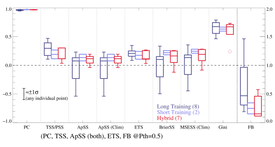
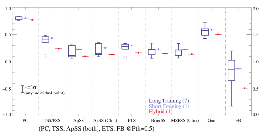
Figure 1: Results from the direct comparison of flare forecasting methods, as grouped by differences in the training interval used, as indicated, for the M1.0+/0/24 event definition (top) and C1.0+/0/24 event definition (bottom). Box & whisker plots are used here, with the mid-line indicating the median, boxes indicating the 25th and 75th percentiles, the whiskers indicating maximum and minimum except circles showing those points beyond 1.5$\times$IQR (the InterQuartile Range). The number of methods represented in each category is indicated with the category color/label. The metrics are those described and presented in Paper II; of note, the Frequency Bias (FB) is on a different scale, referencing the axis on the right. CLIM120 and NJIT are not included in this graphical analysis (see text). Fewer methods provide C1.0+/0/24 forecasts, hence the sparseness of the points relative to the M1.0+/0/24 event definition.

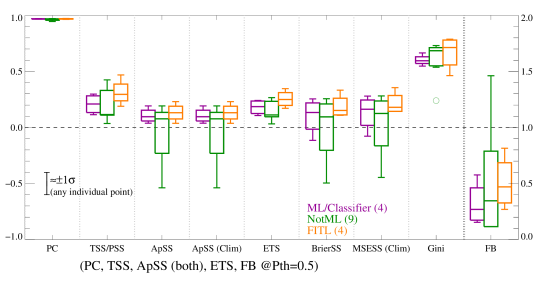
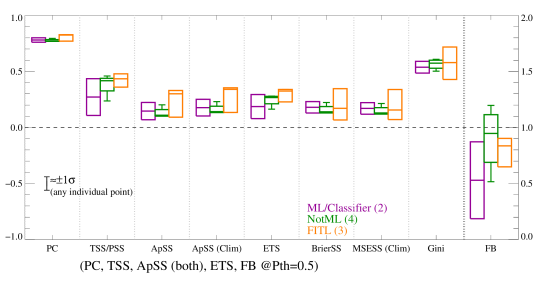
Figure 2: Same as Figure 1, but for comparisons of the methods by which the forecasts are produced, as indicated.

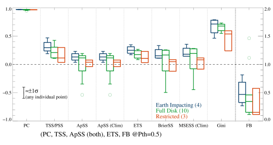
Figure 3: Same as Figure 1, but for comparisons of the zones for which a forecast is issued, as indicated.

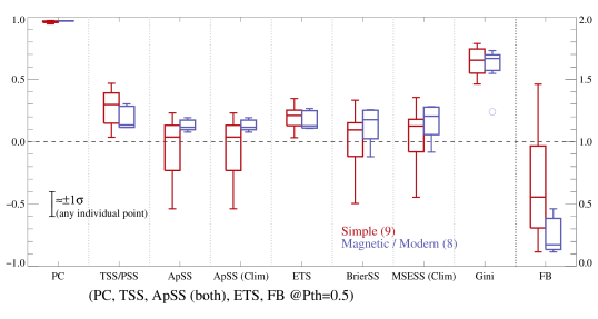
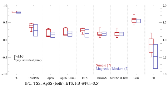
Figure 4: Same as Figure 1, but for comparisons of the parameters or data analysis used by the forecasts, as indicated.

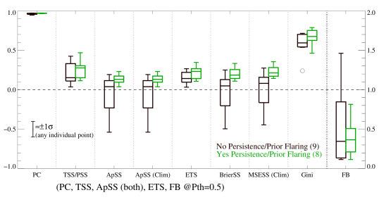
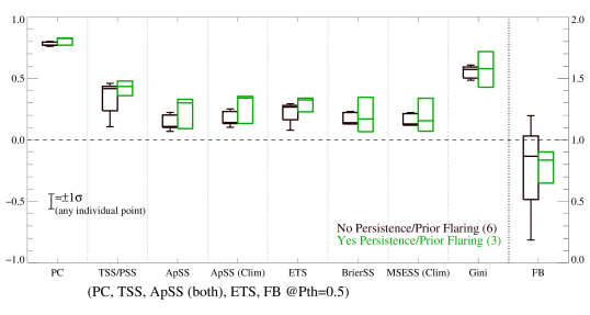
Figure 5: Same as Figure 1, but for the use of flare history or persistence in the forecasts, as indicated.

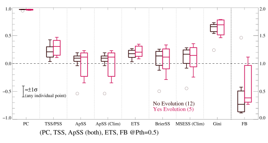
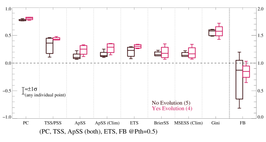
Figure 6: Same as Figure 1, but for the explicit use of active region evolution, as indicated.

There are groups of methods which are similar enough across their implementation that we may draw some interpretations. In doing so we refer to both the figures in this paper and the results and figures in Paper II.

First, the FITL methods were classified identically across our characteristics groupings. They generally employ similar tools at the outset, those being long-trained historical flaring rates following region classification according to size, complexity, etc. (McIntosh, 1990; Sawyer et al., 1986). Differences between methods do arise through the additional tools – both quantitative and qualitative – that are available at each center, but we did not track those differences. All FITL centers commonly have access to (and fully utilize) a very wide selection of data sources; the humans subjectively incorporate the presence of bright beyond-limb emission or other indications of activity sources beyond the visible disk to extend forecasts to beyond that from just the visible magnetic active regions. The final input comes from humans. Other studies have examined the degree of influence that human input imparts to their facility’s initial automated forecasts (Devos et al., 2014; Crown, 2012; Murray et al., 2017). The general trend between those studies and here is consistent: human forecasters in the loop add some skill. Automated methods may be able to incorporate many of these human-brought aspects to their forecasts in due time but, as of yet, none do effectively.

Second, AMOS and MCEVOL are classified identically (MCSTAT differing only in the lack of incorporating evolution); morphologically their Reliability Plots and ROC plots (Paper II Figures 2 and 3) appear similar. While the MCEVOL scores significantly worse on the climatology-referenced metrics than AMOS or MCSTAT (i.e., the ApSS- and MSESS-based metrics), of interest here is that these three are the only “Long” training-interval methods that do not employ some other advancement such as machine learning, persistence, or FITL. The “Long” training-interval methods show some detriment or longer negative-skill extents for some metrics. In conjunction with the performance of the known members of the group, this pattern leads to the conclusion that solely relying on historical flaring rates (plus consideration for just active region growth) is insufficient for successful forecasting. An underlying reason may be the influence of varying climatology, in that these three methods heavily rely upon prior-cycle training when the climatological flaring rate was significantly higher than during our testing period; additionally, MCSTAT and MCEVOL train using data from SC22 while AMOS does not. Training during a period of higher climatology and forecasting during a period of lower flaring rate can lead to overforecasting, and this situation may poignantly demonstrate of the impact of variable climatology (McCloskey et al., 2018).

Two methods lie at the other end of automation, with DAFFS and BOM the sole members of the “Short”-training group. Both rely primarily on high-quality (SDO/HMI) data and magnetic or modern parametrizations, include measures of prior flaring, and employ ML/statistical classifier tools. They tend to under-forecast according to the FB metric (DAFFS slightly less so, see Paper II Figure 4), but perform similarly in other metrics (for the M1.0+/0/24 grouping, since BOM does not provide C1.0+/0/24 forecasts). If one accounts for the performance of the other members of the “ML/Classifier” group, it strengthens the support for a conclusion that there is significant overall skill brought by the combination of approaches illustrated by these two methods.

All FITL centers also have protocols (often some form of climatology) for providing a default or “fall-back” forecast; there are no outtages. This is a quality that some of the automated methods have invoked through repeating the prior forecast, falling back to climatology or, in the case of DAFFS, a progression to DAFFS-G, persistence-measures only, and finally to climatology upon worsening data availability. The performance of methods that lack a default forecast is penalized by the evaluations carried out here and, as discussed in Paper II, can be symptomatic of a marked difference between the research and operational phases of a method.

4 Discussion

We examine the performance of operational flare-forecasting facilities over a standardized testing interval and using standardized event definitions, with the tools of quantitative evaluation metrics. The limited number of events over the testing interval plus the limited number of distinctly different methods make it difficult to draw firm conclusions. However, upon examining the results according to particular implementation techniques and details, a few trends emerge.

The strongest results show that, operationally, the long-held “forecaster’s wisdom” of forecasting increased flare probability from complex and evolving active regions that flared previously is fairly successful. In some cases there are methods that now put these characteristics onto a quantitative basis, although for other methods these aspects are still only incorporated qualitatively. While there is still a spread for some metrics and not fully consistent behavior across all metrics, this appears to be a clear trend.

The use of modern data (such as from the SDO/HMI instrument) or the quantitative analysis of magnetic field data appears to have no significant effect on the performance, providing no obvious advantages at this point but also providing no disadvantages.

Modern statistical methods are now employed in a number of ways for operational forecasting. A few methods have used machine-learning techniques to identify and classify sunspot groups, others use machine-learning algorithms and statistical classifiers to quantify the parameter-space behavior of active regions. Those methods in the former category, however, then generally rely on a Poisson-statistics based analysis of historical flare rates, while there are only three methods that presently incorporate machine learning for the forecast production itself. As such, the sample sizes and limitations of this comparison mean that we cannot comment on any advantages of machine learning in operational flare forecasting.

That being said, the over-arching result of both Paper II and the present study is that none of the current operational flare forecasting methods perform exceptionally well across all performance metrics. However, we may begin to understand some reasons behind particularly poor or particularly good performance in some cases.

Most notably, this study is the first systematic demonstration of how to engage in head-to-head comparisons of operational forecasting models in order to recognize useful trends for future improvements and development. We extend this further in Paper IV (Park et al., 2019) with a new method that focuses on temporal patterns of forecasting errors. Lessons learned from this community effort can help guide future efforts to compare forecasts (such as forecasts collected by the NASA/CCMC Flare Scoreboard) and perhaps help solidify the understanding of what approaches significantly improve performance.

Appendix A Participating Methods and Facilities

In Table 6 we reproduce an abbreviated version of Table 1 from Paper II, listing the methods and facilities involved with this work and the monikers used to refer to them.

Table 6: Participating Operational Forecasting Methods (Alphabetical by Label Used)

Institution	Method/Code Name	Label	Reference(s)
ESA/SSA A-EFFORT Service	Athens Effective Solar Flare Forcasting	A-EFFORT	Georgoulis & Rust (2007)
Korean Meteorological Administration & Kyung Hee University	Automatic McIntosh-based Occurrence probability of Solar activity	AMOS	Lee et al. (2012b)
University of Bradford (UK)	Automated Solar Activity Prediction	ASAP	Colak & Qahwaji (2008, 2009)
Korean Space Weather Center (by SELab, Inc)	Automatic Solar Synoptic Analyzer	ASSA	Hong et al. (2014), Lee et al. (2013)
Bureau of Meteorology (Australia)	FlarecastII	BOM	Steward et al. (2011, 2017)
120-day No-Skill Forecast	Constructed from NOAA event lists	CLIM120	Sharpe & Murray (2017)
NorthWest Research Associates (US)	Discriminant Analysis Flare Forecasting System	DAFFS	Leka et al. (2018)
” ”	GONG+GOES only	DAFFS-G	” ”
NASA/Marshall Space Flight Center (US)	MAG4 (+according to	MAG4W	Falconer et al. (2011);
” ”	magnetogram source	MAG4WF	also see Paper II, Appendix A
” ”	and flare-history	MAG4VW
” ”	inclusion)	MAG4VWF
Trinity College Dublin (Ireland)	SolarMonitor.org Flare Prediction System (FPS)	MCSTAT	Gallagher et al. (2002); Bloomfield et al. (2012)
” ”	FPS with evolutionary history	MCEVOL	McCloskey et al. (2018)
MetOffice (UK)	Met Office Space Weather Operational Center human-edited forecasts	MOSWOC	Murray et al. (2017)
National Institute of Information and Communications Technology (Japan)	NICT-human	NICT	Kubo et al. (2017)
New Jersey Institute of Technology (UK)	NJIT-helicity	NJIT	Park et al. (2010)
NOAA/Space Weather Prediction Center (US)		NOAA	Crown (2012)
Royal Observatory Belgium Regional Warning Center	Solar Influences Data Analysis Center human-generated	SIDC	Berghmans et al. (2005); Devos et al. (2014)

Appendix B Acronyms

Acronyms and references used in Tables 1–4 are expanded upon here.

• AIA: Atmospheric Imaging Assembly (on SDO) (Title et al., 2006)

• ApSS: Appleman Skill Score

• AR: Active Region

• BrierSS: Brier Skill Score

• CM: Central Meridian

• ETS: Equitable Threat Score

• EUVI: Extreme Ultraviolet Imager (on STEREO) (Wuelser et al., 2004)

• FB: Frequency Bias

• FD: Full Disk

• GOES: Geostationary Observing Earth Satellite (run by NOAA)

• GONG: Global Oscillations Network Group (Hill et al., 2003)

• HARP: HMI Active Region Patch (Hoeksema et al., 2014; Bobra et al., 2014)

• HMI: Helioseismic and Magnetic Imager (Hoeksema et al., 2014)

• MSESS: Mean Square Error Skill Score

• NRT: Near Real Time (data)

• PC: Proportion Correct (also known as Rate Correct)

• PDE: Probability Density Estimate

• PROBA2/SWAP: PRoject for Onboard Autonomy / Sun Watcher using Active Pixel System detector and Image Processing

• SC: Solar Cycle

• SDO: Solar Dynamics Observatory (Pesnell, 2008)

• SHARP parameters: pre-computed “Space Weather HARP” parameters describing the magnetic field of HARP regions (e.g. total unsigned magnetic flux, total unsigned vertical current, etc. (Bobra et al., 2014)

• SOON: Solar Optical Observing Network

• SRS: Solar Region Summary, data product of NOAA/SWPC listing active-region attributes.

• STEREO: Solar TErrestrial RElations Observatory (Kaiser et al., 2008)

• TSS: True Skill Statistic (also known by Peirce Skill Score ‘PSS’, Hanssen & Kuiper Skill Score ‘H&KSS’,

• USAF: US Air Force

• Zpc: Modified Zurich Classifications of sunspot groups

References

- Barnes et al. (2016) Barnes, G., Leka, K. D., Schrijver, C. J., et al. 2016, ApJ, 829, 89, doi: 10.3847/0004-637X/829/2/89
- Berghmans et al. (2005) Berghmans, D., van der Linden, R. A. M., Vanlommel, P., et al. 2005, Annales Geophysicae, 23, 3115, doi: 10.5194/angeo-23-3115-2005
- Bloomfield et al. (2016) Bloomfield, D. S., Gallagher, P. T., Marquette, W. H., Milligan, R. O., & Canfield, R. C. 2016, Sol. Phys., 291, 411, doi: 10.1007/s11207-015-0833-6
- Bloomfield et al. (2012) Bloomfield, D. S., Higgins, P. A., McAteer, R. T. J., & Gallagher, P. T. 2012, ApJL, 747, L41, doi: 10.1088/2041-8205
- Bobra et al. (2014) Bobra, M. G., Sun, X., Hoeksema, J. T., et al. 2014, Sol. Phys., 289, 3549, doi: 10.1007/s11207-014-0529-3
- Centeno et al. (2014) Centeno, R., Schou, J., Hayashi, K., et al. 2014, Sol. Phys., 289, 3531, doi: 10.1007/s11207-014-0497-7
- Colak & Qahwaji (2008) Colak, T., & Qahwaji, R. 2008, Sol. Phys., 248, 277, doi: 10.1007/s11207-007-9094-3
- Colak & Qahwaji (2009) —. 2009, Space Weather, 7, 6001, doi: 10.1029/2008SW000401
- Crown (2012) Crown, M. D. 2012, Space Weather, 10, 6006, doi: 10.1029/2011SW000760
- Devos et al. (2014) Devos, A., Verbeeck, C., & Robbrecht, E. 2014, Journal of Space Weather and Space Climate, 27, A29, doi: 10.1051/swsc/2014025
- Falconer et al. (2011) Falconer, D., Barghouty, A. F., Khazanov, I., & Moore, R. 2011, Space Weather, 9, 4003, doi: 10.1029/2009SW000537
- Gallagher et al. (2002) Gallagher, P., Moon, Y. J., & Wang, H. 2002, Sol. Phys., 209, 171
- Georgoulis et al. (2008) Georgoulis, M. K., Raouafi, N.-E., & Henney, C. J. 2008, in Astronomical Society of the Pacific Conference Series, Vol. 383, Subsurface and Atmospheric Influences on Solar Activity, ed. R. Howe, R. W. Komm, K. S. Balasubramaniam, & G. J. D. Petrie, 107
- Georgoulis & Rust (2007) Georgoulis, M. K., & Rust, D. M. 2007, ApJL, 661, L109, doi: 10.1086/518718
- Hill et al. (2003) Hill, F., Bolding, J., Toner, C., et al. 2003, in ESA Special Publication, Vol. 517, GONG+ 2002. Local and Global Helioseismology: the Present and Future, ed. H. Sawaya-Lacoste, 295–298
- Hoeksema et al. (2014) Hoeksema, J. T., Liu, Y., Hayashi, K., et al. 2014, Sol. Phys., 289, 3483, doi: 10.1007/s11207-014-0516-8
- Hong et al. (2014) Hong, S., Kim, J., Han, J., & Kim, Y. 2014, AGU Fall Meeting Abstracts, SH21A
- Kaiser et al. (2008) Kaiser, M. L., Kucera, T. A., Davila, J. M., et al. 2008, Space Science Reviews, 136, 5, doi: 10.1007/s11214-007-9277-0
- Kubo et al. (2017) Kubo, Y., Den, M., & Ishii, M. 2017, Journal of Space Weather and Space Climate, 7, A20, doi: 10.1051/swsc/2017018
- LaBonte et al. (2007) LaBonte, B. J., Georgoulis, M. K., & Rust, D. M. 2007, apj, 671, 955, doi: 10.1086/522682
- Lee et al. (2012a) Lee, K., Moon, Y.-J., Lee, J.-Y., Lee, K.-S., & Na, H. 2012a, Sol. Phys., 281, 639, doi: 10.1007/s11207-012-0091-9
- Lee et al. (2012b) —. 2012b, Sol. Phys., 281, 639, doi: 10.1007/s11207-012-0091-9
- Lee et al. (2013) Lee, S., Lee, J., & Hong, S. 2013, ASSA GUI User Manual, Version 1.07, http://www.spaceweather.go.kr/images/assa/ASSA_GUI_MANUAL.pdf
- Leka et al. (2017) Leka, K. D., Barnes, G., & Wagner, E. L. 2017, Sol. Phys., 292, 36, doi: 10.1007/s11207-017-1057-8
- Leka et al. (2018) —. 2018, Journal of Space Weather and Space Climate, 8, A25, doi: 10.1051/swsc/2018004
- Leka et al. (2019) Leka, K. D., Park, S. H., Kusano, K., et al. 2019, ApJ, submitted
- McCloskey et al. (2016) McCloskey, A. E., Gallagher, P. T., & Bloomfield, D. S. 2016, Sol. Phys., 291, 1711, doi: 10.1007/s11207-016-0933-y
- McCloskey et al. (2018) —. 2018, Journal of Space Weather and Space Climate, 8, A34, doi: 10.1051/swsc/2018022
- McIntosh (1990) McIntosh, P. S. 1990, Sol. Phys., 125, 251
- Murray et al. (2017) Murray, S. A., Bingham, S., Sharpe, M., & Jackson, D. R. 2017, Space Weather, 15, 577, doi: 10.1002/2016SW001579
- Park et al. (2010) Park, S.-H., Chae, J., & Wang, H. 2010, ApJ, 718, 43, doi: 10.1088/0004-637X/718/1/43
- Park et al. (2019) Park, S. H., Leka, K. D., Kusano, K., et al. 2019, ApJ, in preparation
- Pesnell (2008) Pesnell, W. 2008, in COSPAR, Plenary Meeting, Vol. 37, 37th COSPAR Scientific Assembly, 2412
- Sawyer et al. (1986) Sawyer, C., Warwick, J. W., & Dennett, J. T. 1986, Solar Flare Prediction (Boulder, CO: Colorado Assoc. Univ. Press)
- Schou et al. (2012) Schou, J., Scherrer, P. H., Bush, R. I., et al. 2012, Sol. Phys., 275, 229, doi: 10.1007/s11207-011-9842-2
- Sharpe & Murray (2017) Sharpe, M. A., & Murray, S. A. 2017, Space Weather, 15, 1383, doi: 10.1002/2017SW001683
- Steward et al. (2017) Steward, G., Lobzin, V., Cairns, I. H., Li, B., & Neudegg, D. 2017, Space Weather, 15, 1151, doi: 10.1002/2017SW001595
- Steward et al. (2011) Steward, G. A., Lobzin, V. V., Wilkinson, P. J., Cairns, I. H., & Robinson, P. A. 2011, Space Weather, 9, S11004, doi: 10.1029/2011SW000703
- Title et al. (2006) Title, A. M., Hoeksema, J. T., Schrijver, C. J., & The AIA Team. 2006, in COSPAR, Plenary Meeting, Vol. 36, 36th COSPAR Scientific Assembly, 2600
- Wuelser et al. (2004) Wuelser, J.-P., Lemen, J. R., Tarbell, T. D., et al. 2004, in Society of Photo-Optical Instrumentation Engineers (SPIE) Conference Series, Vol. 5171, Telescopes and Instrumentation for Solar Astrophysics, ed. S. Fineschi & M. A. Gummin, 111–122