Geodesic Learning via Unsupervised Decision Forests

Geodesic distance is the shortest path between two points in a Riemannian manifold. Manifold learning algorithms, such as Isomap, seek to learn a manifold that preserves geodesic distances. However, such methods operate on the ambient dimensionality, and are therefore fragile to noise dimensions. We developed an unsupervised random forest method (URerF) to approximately learn geodesic distances in linear and nonlinear manifolds with noise. URerF operates on low-dimensional sparse linear combinations of features, rather than the full observed dimensionality. To choose the optimal split in a computationally efficient fashion, we developed a fast Bayesian Information Criterion statistic for Gaussian mixture models. We introduce geodesic precision-recall curves that quantify performance relative to the true latent manifold. Empirical results on simulated and real data demonstrate that URerF is robust to high-dimensional noise, whereas other methods, such as Isomap, UMAP, and FLANN, quickly deteriorate in such settings. In particular, URerF is able to estimate geodesic distances on a real connectome dataset better than other approaches.

Introduction

Learning to organize, rank, and sort points from a data corpus is a fundamental challenge in data science, and a statistical primitive underlying many computer science and machine learning tasks. For example, nearest neighbor algorithms, which sort all points according to their distances to one another, are considered among the top 10 most important algorithms of all time [1], and have strong theoretical guarantees for both classification and regression [2]. Decision trees (such as CART and C4.5) can also reasonably be thought of as algorithms for organizing data in a hierarchical fashion; these are among the top ten algorithms as well [1]. Moreover, decision trees underlie both random forests [3] and gradient boosted trees [4], which are the two leading algorithms for machine learning on tabular data today [5, 6, 7]. To complement the above supervised machine learning settings, there is a rich literature on approximate nearest neighbor algorithms (see Aumüller et al. [8] for benchmark comparisons of many state of the art approaches), which are used extensively in big data systems.

Operating on the exact nearest neighbors, (or trying to approximate them), is not always desirable. For example, consider a simplest supervised learning setting. Given a data corpus, $\{(x_{n},y_{n})\}_{n=1}^{N}$, learn a decision rule such that, given a new data point $x$, its prediction of $y$ has small error with high probability. A canonical approach is kernel regression [9]. A kernel machine’s prediction is a weighted linear combination of predictions that the neighbors of $x$ would make, specifically, $\hat{y}=\frac{1}{N}\sum_{n=1}^{N}y_{n}\times\kappa(x,x_{n})$, for some suitably chosen kernel $\kappa$ (for example, a radial basis function or $k$-nearest neighbors kernel). Such approaches enjoy strong theoretical guarantees [10]. Now, further assume that the $x$’s are noisy measurements of some true, but unobserved $\tilde{x}$’s. Such an assumption, called “measurement error modeling” [11], could reasonably be argued to be much more accurate than assuming the $x$’s are noise-free measurements [12]. Under this measurement error assumption, a better approach—meaning an approach that likely achieves smaller error given the same sample size—would be a kernel regression function on the noise-free measurements, $\hat{y}=\frac{1}{N}\sum_{n=1}^{N}y_{n}\times\kappa(\tilde{x},\tilde{x}_{n})$. Unfortunately, because the $\tilde{x}$’s are not observed, such an approach is not available. This modeling framework therefore motivates learning the latent structure of the data, even for low-dimensional data. In particular, it motivates learning which sample points are close to one another on an underlying latent structure (such as a manifold), for subsequent inference. Moreover, even though the above task is a supervised learning task, performance improves when learning the structure of only the features $x$, while not even considering the labels $y$ .

Learning latent structure is even more important in the “large p, small N” setting. Specifically, when the dimensionality $p$ is larger than the sample size $N$, an intermediate representation is required to avoid (1) numerical stability issues with matrix operations, and (2) the “curse of dimensionality” for statistical operations. This intermediate representation can be explicit (as in manifold learning) or implicit (as in kernel machines). When $N$ is large, even approximation algorithms are required to compute various quantities whose exact solution requires $\mathcal{O}(N^{2})$ or $\mathcal{O}(N^{3})$ space and/or time.

Geodesic learning is the process of estimating geodesic distances between pairs of points in a data corpus. It is crucial (though sometimes implicit) in many state-of-the-art machine learning algorithms. For example, the first step in many manifold learning algorithms is to estimate the geodesic distance between all pairs of points [13]. Nonetheless, scant work explicitly addresses geodesic learning, perhaps because in any real data application the true geodesic distances are not observed, or because a suitable metric for evaluating geodesic learning is not currently available. Despite this, several disciplines in computer science and machine learning have developed strategies to partially address the challenges associated with geodesic learning.

In computer science, space-partitioning trees are used extensively for quite diverse applications; most relevant to this work are efforts to build trees in support of efficient geometric queries [14]. Commonly, space partitioning trees use binary and recursive splits with hyperplanes [15]. These tree structures are usually optimized to learn relative proximities of the observed, noisy measurements, rather than the latent noise-free, and potentially lower dimensional, measurements. These partition trees from data structures are closely related to decision trees developed in statistics and machine learning [16]. In fact, extensions to decision trees are established as the de facto standard for classification and regression tasks (even in this age of deep learning), including random forests [3] and gradient boosting trees [17]. These approaches, however, are almost exclusively concerned with supervised, rather than unsupervised learning. Decision trees have always been linked to kernel learning [18], a realization that recently gained traction in the machine learning literature [19, 20, 21, 22]. Kernel machines typically assume a kernel, or select one from a finite set or one-dimensional family of kernels, limiting their finite sample performance. In manifold learning, many spectral variants start by estimating all pairwise geodesic distances [23]. These approaches typically operate on the observed, typically high-dimensional data, and therefore suffer serious drawbacks in the face of additional noise dimensions. Although each of the above works is closely related to geodesic learning, to our knowledge none of it explicitly aims to estimate geodesic distances as an end unto itself. Moreover, those approaches that do estimate geodesic distances typically do not directly evaluate the estimated distances.

We propose Unsupervised Randomer Forest (URerF) to achieve near linear space and time complexity, while approximating the true latent geodesic distances. Unlike the previously described methods, URerF does not need to compute geodesic distances between all pairs of points. Instead, URerF examines local structure by recursively clustering data in sparse linear subspaces, building on the recently proposed randomer forest algorithm for supervised learning [24]. The randomer forest approach allows URerF to separate meaningful structure in the data from the noise dimensions. We also introduce a spitting criteria, Fast-BIC, which efficiently and exactly computes the Bayesian Information Criterion statistic for an approximate Gaussian mixture model in one dimension.

This manuscript also contributes a method for evaluating geodesic learning algorithms. Most existing manuscripts on manifold learning that explicitly estimate geodesic distances, do not explicitly evaluate the geodesics. Rather, such papers typically embed the data into some low-dimensional space and then visualize the results. This approach is limited in a number of ways: (1) it is qualitative; (2) when the structure is higher dimensional it may be revealed by the first few dimensions; and (3) it relies on an embedding, which introduces additional computational and statistical complications. Sometimes the embedded data are used for subsequent inference tasks, such as classification, which can be quantitatively evaluated. Such an approach is only able to evaluate performance of a manifold learning algorithm composed with a particular subsequent inferential method, but not the manifold or geodesic learning algorithms directly.

We therefore introduce geodesic precision and recall. In contrast to precision and recall as typically defined, geodesic precision and recall quantify the set of nearest neighbors as estimated by the geodesic learning algorithm, with the set of true nearest neighbors on the latent manifolds. As a general rule, if a geodesic learning algorithm does poorly on this metric, estimating manifolds from these geodesics has no hope to perform well on subsequent tasks. Indeed, functions of geodesic precision can provide tight bounds on subsequent classification accuracy [25].

URerF finds neighbors in the latent low-dimensional space amid additional noise dimensions more effectively than other approaches. Moreover it can do this in a variety of linear and nonlinear settings, with different dimensional submanifolds, and in a real connectome dataset.

Related Work

Nonlinear manifold learning approaches, such as Isomap [26], Laplacian eigenmaps [27] and UMAP [28], are designed to preserve geodesic distances, and even directly estimate them. Specifically, they follow a three-step process. First, they estimate geodesic distances in the original manifold. This is done by initially constructing a $k$-nearest neighbor or $\epsilon$-neighborhood graph in which the observations (data points) correspond to nodes, and pairwise Euclidean distances between these points correspond to the weights on the edges. Second, the all-pairs shortest paths of the nodes in the graph are computed. Third, the points are embedded in a lower dimensional space that ideally preserves these distances. This approach is significantly hampered by the first step, which operates in the original high-dimensional ambient space, since Euclidean distances often fail to provide good estimates of distances on the manifold. Moreover, given $n$ datapoints, computing all pairwise distances is $\mathcal{O}(n^{2})$ space and time, and all pairwise shortest paths can require $\mathcal{O}(n^{3})$, both of which can be cost prohibitive for large sample sizes.

One of the most widely used methods for nonlinear dimensionality reduction is Isomap [26]. Isomap is one of the few manifold learning algorithms that has theoretical guarantees for correctly estimating the manifold under certain assumptions [29]. In the case of many noisy dimensions, however, Isomap fails to construct an accurate nearest-neighbor graphs on the latent manifold. Moreover, Isomap requires storing all point-to-point graph distances, which incurs space and time complexity quadratic in the sample size.

UMAP is a new algorithm for dimensionality reduction that efficiently reduces high-dimensional data to a low dimension using a fuzzy simplicial set representation of the input data points [28]. Like other nearest-neighbor based algorithms, UMAP first constructs an undirected, weighted k-nearest neighbor graph from the input data, then embeds data points in a low-dimensional space using a force-directed layout algorithm. The number of neighbors used to construct the graph in effect determines the local manifold structure that is to be preserved in the low-dimensional layout. In the force-directed layout approach, attractive forces between close vertices are iteratively balanced with repulsive forces between vertices that are far apart in the graph until convergence. UMAP builds upon the popular t-Distributed Stochastic Neighbor Embedding (t-SNE) algorithm, which attempts to preserve original interpoint distances in a much lower dimensional space [30]. The Kullback-Leibler divergence between the distribution of neighbor distances in the higher and lower dimensional spaces is used to determine the optimal mapping of points into the lower-dimensional space. t-SNE is primarily used to visualize high-dimensional data [31], and cannot be used with non-metric distances. The UMAP algorithm produces similar embeddings to t-SNE in two or three dimensions, but scales better in terms of run-time across a wide range of embedding dimensions [28].

Approximate nearest neighbors algorithms, such as FLANN [32], approximate nearest-neighbors in high-dimensional data sets, typically by building binary space-partitioning trees, such as $K$-d trees. These algorithms are designed to estimate the distances in the observed high-dimensional space. When the true manifold is low-dimensional, and the data are high-dimensional, the additional noise dimensions will be problematic for any of these algorithms. On the other hand, these approaches can achieve near linear space and time complexity.

This work is inspired by, and closely related to, random projection trees for manifold learning [33] and vector quantization [34]. The main differences between our approach and theirs is (1) that they use random splits, rather than optimizing the splits; and (2) they use a single tree, whereas URerF uses a forest of many trees. Nonetheless, their theoretical analysis motivates the geodesic precision metric we establish for quantifying performance of geodesic learning.

Finally, most closely related to our method are existing unsupervised random forest methods, the most popular of which is included in Adele Cutler’s RandomForest R package [35]. It proceeds by generating a synthetic copy of the data by randomly permuting each feature independently of the others, and then attempts to classify the real versus the synthetic dataset. As will be seen below, this approach leads to missing surprisingly easy latent structures.

Unsupervised Randomer Forests

A random forest is an ensemble of decision trees in which each tree is created from bootstrapped samples of the training dataset; that is, each tree is built from a random subset of training data. Each tree $\{h(\textbf{x},\theta_{t})\},t\in\{1,2,\ldots,T\}$ has parameters $\theta_{t}$ that characterize the tree structure, and can be learned from the dataset. Given a set of trees, and a new point $x$, each tree casts a unit vote for its predictions given the input x. Typically, random forests are used in supervised machine learning tasks, specifically classification and regression. There have been a few papers reporting on unsupervised random forests for certain tasks [36].

Our unsupervised random forest algorithm is based on the original Random Forest algorithm [3] with a few key distinctions. First, URerF uses a new splitting criteria, Fast-BIC, that efficiently and exactly computes an approximate Bayesian Information Criterion for a Gaussian Mixture model in one dimension. Second, we use the term randomer to label our technique, as our splitting methods are based on random sparse linear combinations of features to strengthen each tree, as originally proposed by Breiman [3], and later studied further by Tomita et al. [24, 37] Third, we correctly implement a previously proposed method for generating proximity matrices from random forests. In one of the most widely used implementations of Random Forest [38], the aggregated normalized proximity matrices of $F$ Random Forests with $T$ trees each is not stochastically equivalent to the aggregated normalized proximity matrices of $T$ Random Forests with $F$ trees each. Our implementation does not suffer from this bug. Furthermore, it is computationally more efficient than previous implementations. These three changes enable URerF to achieve state-of-the-art performance on both simulated and real data.

Overall algorithm

Given an input data set $x=\{x_{1},\ldots,x_{N}\}$, where $x_{n}\in\mathbb{R}^{p}$, URerF builds $T$ decision trees, each from a random sample of size $m<N$. In each tree, URerF recursively splits a parent node into its two child nodes until some termination specification is met. At each node, URerF generates $d$ features to search over. Each feature is evaluated based on the splitting criteria described in Section 3.3, and the feature with the best score is selected to split the data points into two daughter nodes. Algorithm 1 describes the procedure used to build unsupervised decision trees (all algorithms are relegated to the appendix). To evaluate the forest, a proximity matrix is then generated by computing the fraction of the trees in which every pair of elements reside in the same leaf node (Section 3.4).

Node-Wise Feature Generation

Unlike Breiman’s original random forest algorithm, URerF does not choose split points in the original feature space. Instead, we follow the random projection framework of Tomita et al. [24, 37]. For $p$-dimensional input data, we sample a $p\times d$ matrix $A$ distributed as $f_{A}$, where $f_{A}$ is the projection distribution and $d$ is the dimensionality of the projected space. We chose to use the $f_{A}$ that Tomita et al. empirically found to produce the best performance in the supervised setting: $A$ is generated by randomly sampling from $\{-1,+1\}$ $\lambda pd$ times, then distributing these values uniformly at random in $A$ [24]. The $\lambda$ parameter is used to control the sparsity of $A$, and is set to $\frac{1}{20}$, again following the convention of Tomita et al. Using the randomly sampled $p\times d$ matrix $A$, the data associated with the given node, $X^{\prime}$, which is a subsample of the original data, is transformed into a $d$-dimensional feature space, where each of the $d$ new features is now a sparse linear combination of the $p$ original features. In other words, each row of $\tilde{X}=A^{T}X^{\prime}$ represents a projection of the data into a one-dimensional space that is a sparse linear combination of the original feature space. Each of the $d$ rows $\tilde{X}[i,:],i\in\{1,2,...,d\}$ is then inspected for the best split point. The optimal split point and splitting dimension are chosen according to which point/dimension pair minimizes the splitting criteria described in the following section.

Splitting Criteria

Fast, Exact, Univariate, Two-Means Splitting

The goal is to find the split that minimizes the sum of the intra-cluster variance on the projected dimension. Typically, k-means problems are solved via Ward’s or Hardigan’s algorithms [39, 40]. Because k-means is NP-hard, in general, these algorithms lack strong theoretical guarantees [41]. However, in one-dimension, for two-means, there is an exact solution that is much faster and simpler. This is available because each decision tree always operates on one-dimensional marginals. First, sort the data points. Then, consider splitting between all sequential pairs of points; that is, letting $x_{(s)}$ denote the $s^{th}$ smallest sample, consider splitting between $x_{(s)}$ and $x_{(s+1)}$ for all $s<N$. The samples to the left of the split point form one cluster, and those to the right form the other cluster. Estimate the means for each of the clusters using the maximum likelihood estimate (MLE) for all points in that cluster. Fast, exact, univariate two-means splitting seeks to find the cutpoint that minimizes the one-dimensional 2-means objective. This splitting criteria was introduced in [33].

$$\min_{s}\sum_{n=1}^{s}(x_{n}-\hat{\mu}_{1})^{2}+\sum_{n=s+1}^{N}(x_{n}-\hat{\mu}_{2})^{2}.$$ (1)

An immediate limitation of this approach is that it fails to consider feature-wise variance, which can lead to undesirable properties. For example, if any feature has zero variance, it will always achieve the minimum possible score. Although one can rescale each feature independently, doing so can cause problems in unsupervised learning problems when the relative scale of features is important, and the details of how to rescale introduce an undesirable algorithm parameter to tune.

2-Gaussian Mixture Model Splitting with Mclust-BIC

In this case, for each feature we fit the data to a two-component Gaussian mixture model (GMM). An expectation-maximization (EM) is used to jointly estimate all the parameters and latent variables [42]. The latent variables, $\{z_{n,j}\}$, denote the probability that sample $n$ is in cluster $j$. Letting $N$ be the number of observations and $J$ be the number of Gaussian clusters (in this case, $J=2$), and introducing notation $x=\left(x_{1},\ldots,x_{N}\right)$, and $z=\{z_{1,1},z_{1,2},\ldots,z_{N,J}\}$, the complete likelihood (including the latent variables) is

$$P(x,z;{\mu},{\sigma},{\pi})=\prod_{n=1}^{N}\prod_{j=1}^{J}\{\pi_{j}\mathcal{N}(x_{n};\mu_{j},\sigma_{j}^{2})\}^{z_{n,j}}.$$ (2)

Each feature is evaluated using the Bayesian Information Criterion (BIC). BIC is based on the log likelihood of the model given the data, with a regularization term penalizing complex models with many parameters. Concretely, letting $\hat{L}_{M}$ denote the maximum log likelihood function of a particular model $M$, $\hat{L}_{M}=p(x;\hat{\theta}_{M})$, where $\hat{\theta}_{M}$ are the parameters that maximize the likelihood function for model $M$, and $x$ is the observed data. Letting $N$ be the sample size (number of data points) and $d_{M}$ be the number of parameters estimated by the model, then the BIC score can be defined as follows:

$$BIC(M)=-2\ln(\hat{L}_{M})+\ln(N)d_{M}.$$ (3)

The feature that maximizes the BIC score for a two-component GMM is selected for splitting at each node. The split occurs at the midpoint where the two Gaussians are equally likely. Because this approach is standard in the literature, we do not provide pseudocode. Note that the EM approximates the actual log likelihood, and is only guaranteed to find a local maximum, not the global maximum, rending it sensitive to initialization. Moreover, the EM algorithm is known to suffer from poor convergence properties in certain settings [43].

2-GMM Splitting with Fast-BIC

Fast-BIC combines the speed of two-means with the model flexibility of Mclust-BIC. As in two-means, for each feature, sort all the data, and try all possible splits. For each split, assign all points below the split to one Gaussian, and all points above the split to the other Gaussian. Estimate the prior, means, and variances for both clusters using the MLE. For $j=1$, they are defined by

$$\hat{\mu}_{1}=\frac{1}{s}\sum_{n\leq s}x_{n},\qquad\hat{\sigma}_{1}=\frac{1}{s}\sum_{n\leq s}||x_{n}-\hat{\mu_{j}}||^{2},\qquad\hat{\pi}_{1}=\frac{s}{N},$$

and similarly for $j=2$. Under the above assumption, $z_{n,j}$ is an indicator that data point $x_{n}$ is in cluster $j$. In other words, rather than the soft clustering of GMM, Fast-BIC performs a hard clustering, as in two-means. Thus, if $x_{n}$ is in cluster $j$, then $z_{n,j}=1$ and $z_{n,j^{\prime}}=0$ for all $j\neq j^{\prime}$. Given this approximation, the likelihood can be obtained by summing over the $z$’s

$$P(x;\mu,\sigma,\pi)=\sum_{z}\prod_{n=1}^{N}\prod_{j=1}^{J}\{\pi_{j}\mathcal{N}(x_{n};\mu_{j},\sigma_{j}^{2})\}^{z_{n,j}}.$$ (4)

Noting that $z_{(n\in(0,s],k=0)}=z_{(n\in[s+1,N),k=1)}=1$ and $z_{n,j}=0$ otherwise, Equation (4) can be simplified to

$$P(x;\mu,\sigma,\pi)=\prod_{n=1}^{s}\pi_{1}\mathcal{N}(x_{n};\hat{\mu_{1}},\sigma_{1}^{2})\prod_{n=s+1}^{N}\pi_{2}\mathcal{N}(x_{n};\hat{\mu_{2}},\sigma_{2}^{2}).$$

Plugging in the MLE for all the parameters, the maximum log likelihood function $\hat{L}=\log P(x;\hat{\mu},\hat{\sigma},\hat{\pi})$ is

$$\hat{L}=\sum_{n=1}^{s}[\log\hat{\pi}_{1}+\log\mathcal{N}(x_{n};\hat{\mu_{1}},\hat{\sigma_{1}}^{2})]+\sum_{n=s+1}^{N}[\log\hat{\pi}_{2}+\log\mathcal{N}(x_{n};\hat{\mu_{2}},\hat{\sigma_{2}}^{2})],$$ (5)

Substituting into Equation 5 and simplifying, we get the following expression for the log likelihood for any given $s$:

$$-2\hat{L}_{s}=s\log 2\hat{\pi}_{1}\hat{\sigma}_{1}^{2}+(N-s)\log 2\hat{\pi}_{2}\hat{\sigma}_{2}^{2}-s\log\hat{\mu_{1}}-(N-s)\log\hat{\mu_{2}},$$ (6)

in which we have dropped terms that are not functions of the parameters. We further test for the single variance case ($\sigma_{1}=\sigma_{2}$) and use the BIC formula to determine the best case. Fast-BIC chooses the dimension and split-point that maximizes $\hat{L}_{s}$. Pseudocode for this approach is provided in Algorithm 3. Fast-BIC is guaranteed to obtain the global maximum likelihood estimator, whereas the Mclust-BIC is liable to find only a local maximum. Moreover, Fast-BIC is substantially faster. This Fast-BIC procedure is, to our knowledge, novel, and of independent interest.

Proximity Matrix Construction

One can build a similarity matrix from any decision tree by asserting that similarity between two points $x_{n}$ and $x_{j}$ is related to some “tree distance” between the pair of points in a given tree. Although this is the case for both supervised an unsupervised decision trees, to our knowledge such an approach has not yet been explored for unsupervised trees. When using a forest, it is natural to average the similarity matrices to obtain the forest’s estimate of similarity. A simple tree distance to use is the $0-1$ loss on whether a pair of points is in the same leaf node. This approach to computing similarities has previously been studied in several supervised random forest papers, connecting random forests to kernel learning [18, 19, 20, 21, 22]. However, the connection between these similarities and geodesic distances has not yet been established.

More concretely, the proximity matrix $S$ for input data $D\in\mathbb{R}^{n\times d}$ is estimated using the unsupervised random forest by simply counting the fraction of times that a pair of points occurs in the same leaf node in the forest. Thus, $S(i,j)=S_{ij}=\frac{L_{ij}}{T_{ij}}$, where $L(i,j)$ is the number of occurrences of points $i$ and $j$ in the same leaf node, and $T_{ij}$ is the number of trees in which both point $i$ and point $j$ were included in the bootstrap sample that was used to build the tree. We use both the in-bag and out-of-bag samples to estimate the proximity.

Geodesic Precision and Recall

Geodesic precision and recall differ from “classical” precision and recall by virtue of defining the neighbors based on the true latent low-dimensional manifold, rather than the observed (typically higher-dimensional) space. The typical definition of precision and recall are defined relative to a query, the relevant samples are those that are “correct”, where as the retrieved samples are those that are returned by the query. Letting $\cap$ denote set intersection, and $|\cdot|$ denote the cardinality of the set, precision and recall are

precision $$=\frac{|\{\text{relevant samples}\}\cap\{\text{retrieved samples}\}|}{|\{\text{retrieved samples}\}|},$$

recall $$=\frac{|\{\text{relevant samples}\}\cap\{\text{retrieved samples}\}|}{|\{\text{relevant samples}\}|}.$$

For geodesic learning, given a data point $x$, a data corpus $\mathcal{D}_{N}=\{x_{1},\ldots,x_{N}\}$, and a query size $k$, the relevant samples are the $k$ samples from $\mathcal{D}_{N}$ that are nearest to $x$ based on the true (but unknown) geodesic distance. In other words, “correct” neighbors is defined by the latent, noise-free, manifold, rather than the observed, typically higher dimensional space. Given a geodesic learner, the retrieved samples are the $k$ samples that the learner reports are nearest. To compute the geodesic precision and recall for a given learner on a given dataset, average the geodesic precision and recall over each sample point. Higher precision and lower recall indicate better estimation of geodesic distances.

We consider two distinct cases: a continuous geodesic, in which there is a finite geodesic distance between all pairs of points, and a discrete geodesic, in which there are clusters of points that are not connected at all to other points. In the latter case (such as a union of spheres), we denote all the points within a given connected component as its neighbors, and all points outside its connected component as not neighbors. In the disconnected setting, geodesic precision and recall are identical to one another.

Numerical Results

Four Multivariate Manifold Simulation Settings

Figure 1: Synthetic datasets for all experiments. In each case, there are 1000 points in 3 signal dimensions, as shown.

We explore geodesic learning using the following four simulations settings, as shown in Figure 1, each of which span a complementary and interesting case. In the linear case, where learning the geodesic should be relatively easy, Euclidean distance will completely recover the geodesics with no noise. It therefore sets an upper bound on performance. The helix setting is reminiscent of the typical “swiss jelly roll” setting popular in manifold learning, but the latent submanifold is one-dimensional embedded into a three-dimensional space. Here, Euclidean will perform poorly, but various manifold learning algorithms should perform well, as they are designed for this kind of scenario. The sphere case is interesting because unlike the helix, the true manifold is two-dimensional and could easily be extended to higher dimensions. Finally, the Gaussian mixture model we suspect will be particularly challenging for the manifold learning algorithms, which typically lack theoretical guarantees for disconnected connected component graphs. Appendix B provides the mathematical details for the four different settings.

Choosing the Splitting Criteria and Robustness to Algorithm Parameters

Figure 2: Geodesic recall curves for the three different splitting criteria using both axis-aligned splits (URF; solid lines) and sparse oblique spits (URerF; dashed lines). In each case there are 1000 points and 3 signal dimensions (no noise dimensions). In general, URerF with Fast-BIC performs the best or nearly so.

Figure 3: Top Geodesic precision versus k for different values of minparent (the smallest splittable node size). Mtry is set to be equal to the square root of the number of features. Bottom Geodesic precision versus k for different values of mtry (the number of features to test at each node). Minparent was set to be equal to 100. Geodesic precision is robust to large variations in these parameters

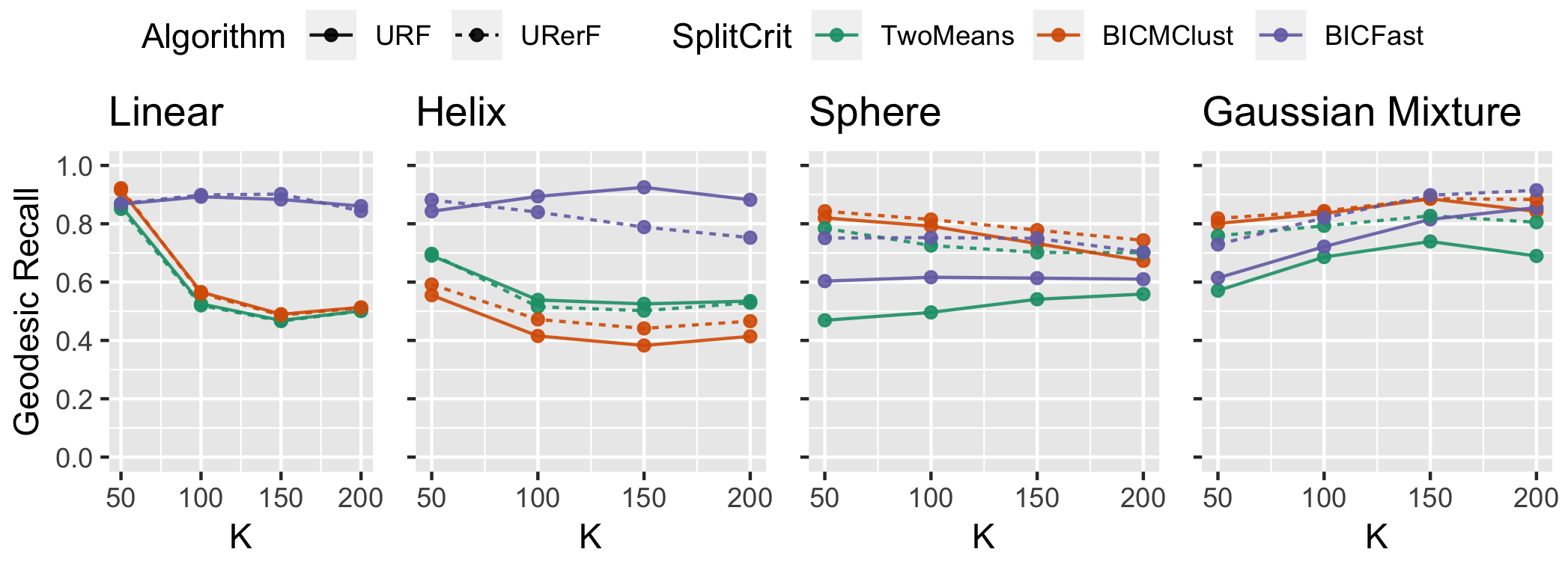
For each of the above simulation settings, we sample a thousands points and calculate the geodesic precision using different unsupervised random forest variants. Figure 2 shows an empirical comparison of the three different splitting criteria described with URF and with URerF. In all cases, both BIC approaches (red and blue) outperform two-means splitting criteria (green). The solid and dashed lines show the relative performance of URF as compared to URerF (URerF use sparse oblique splits, that is, splits on linear combinations of the original features), respectively. In most cases, URerF outperforms URF, as expected based on previous comparisons of sparse oblique splits to axis-aligned splits in supervised random forest [3, 24, 37]. The ramification of these two results is that in all cases, URerF using Fast-BIC performs as well, or nearly as well, as the other options. Because it performs as well as other options, and runs as fast as two-means, we elect to use URerF+Fast-BIC (hereafter, simply URerF) as our unsupervised decision forest splitting criteria.

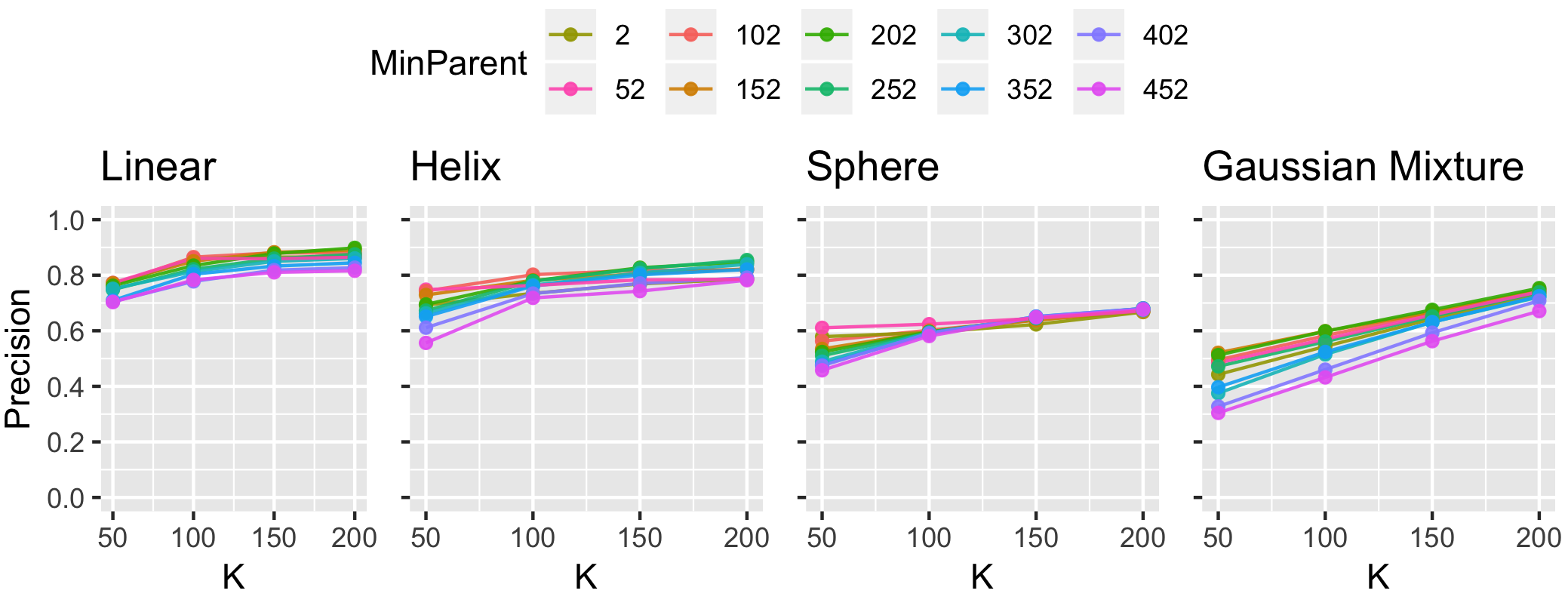
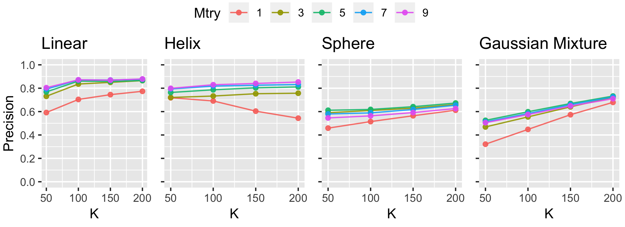
In addition to the splitting criteria, each decision tree has two other important algorithm parameters. First, minparent, which sets the cardinality of the smallest node that might be split. Second, mtry, which is the number of features to test at each node. Figure 3 shows the geodesic precision for different values of minparent and mtry. Geodesic precision using URerF is robust to hyperparameter changes, obviating the need for tuning hyperparameters via a grid search, which can be computationally intensive. For all future experiments, we set minparent to 100 and mtry to $\sqrt{d}$.

URerF is Robust to Noise Dimensions

Figure 4: Top Geodesic precision at k=50 with varying noise dimension from 2 to 10,000, with $N=1000$ samples. While all previous state of the art algorithms degrade to chance levels in all settings as the number of noise dimensions increases, URerF never degrades to chance performance for any of the settings. Bottom Same as top, but each dimension is linearly rescaled to be between 0 and 1, and x-axis shows a smaller number of dimensions (from 0 to 10). Although rescaling greatly improves geodesic precision and recall for most algorithms, URerF still achieves much larger geodesic recall for most settings considered.

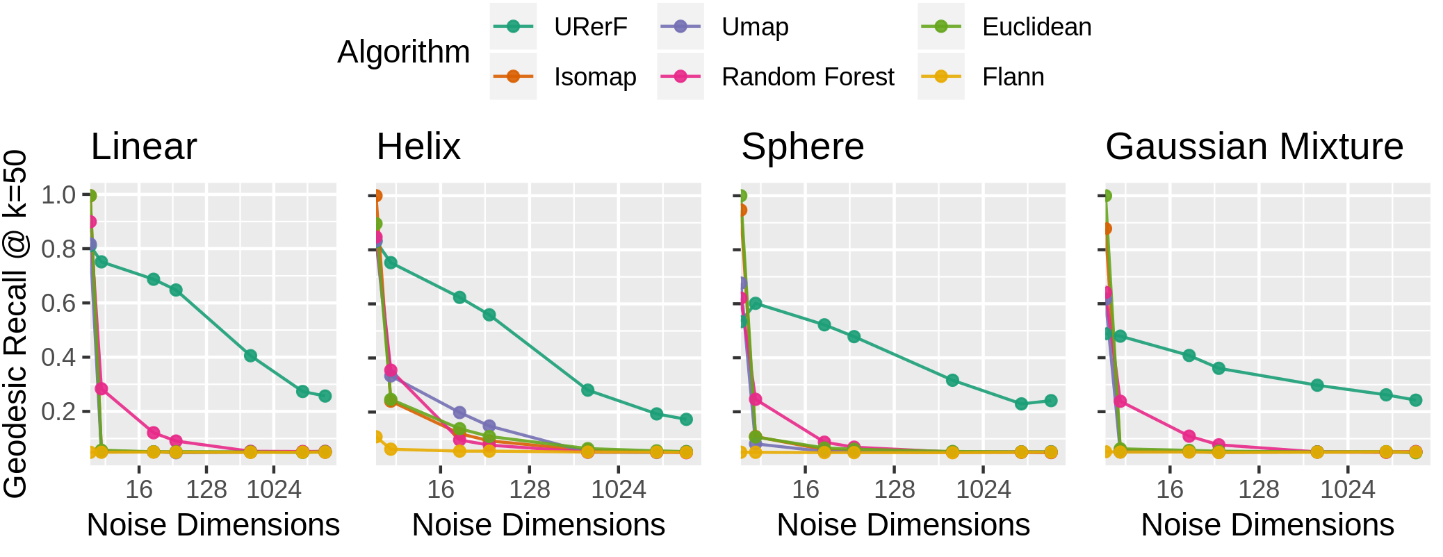
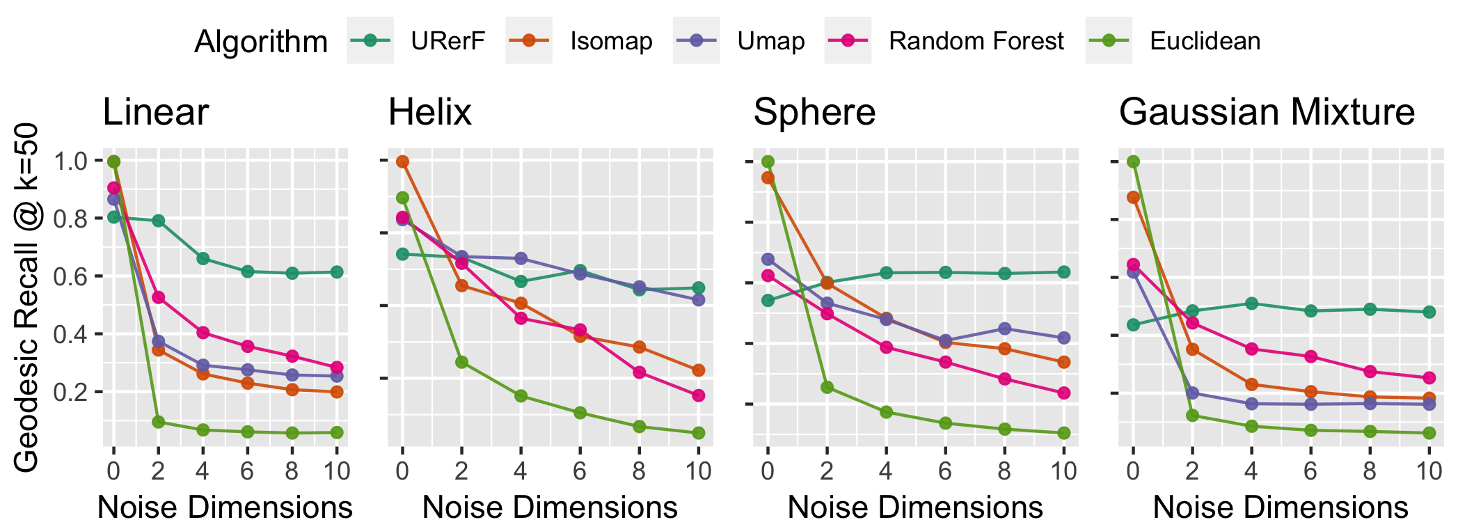
To see that URerF is robust to high dimensional noise, Gaussian noise with varying dimensions $d^{\prime}$ are concatenated onto the simulated datasets. Specifically, for each data point $x_{n}\in\mathbb{R}^{d}$, generated noise $y_{n}\overset{iid}{\sim}\mathcal{N}(0,c\mathbb{I})$ where $y_{n}\in\mathbb{R}^{d^{\prime}}$ is concatenated onto $x_{n}$, ($c=70$ in the following experiments), and $\mathbb{I}$ is the $d^{\prime}\times d^{\prime}$ identity matrix. The new data points with noise are thus: $\tilde{x}_{n}=[x_{n}^{\top}|y_{n}^{\top}]^{\top}\in\mathbb{R}^{d+d^{\prime}}$. Each algorithm’s proximity matrices are computed on the $\tilde{x}$’s, and compared with geodesic distance matrices to obtain geodesic precision and recall.

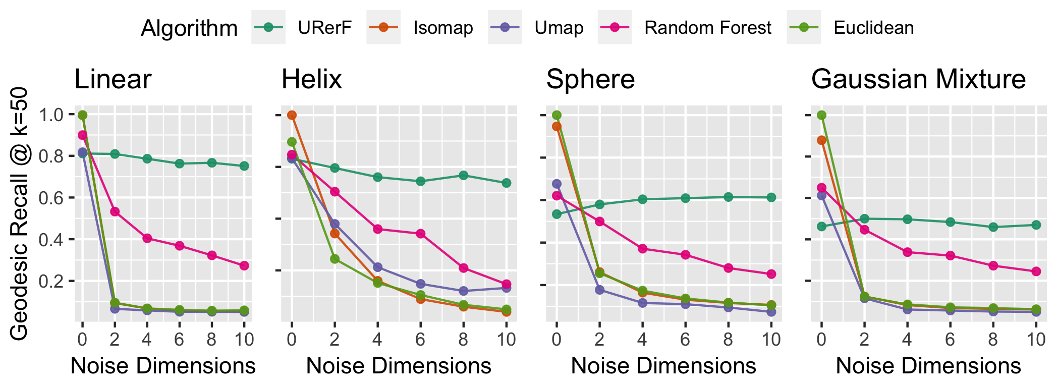
Figure 6 shows the geodesic recall @ k=50 as a function of the number noise dimensions for Isomap, UMAP, random forests, Euclidean distance, FLANN, and URerF. URerF performs well even with the addition of high dimensional noise dimensions. The other state-of-the-art algorithms achieve a higher geodesic recall than URerF in the absence of noise dimensions, but degrade much more quickly than URerF upon the addition of noise dimensions. FLANN and Euclidean distance degrade the fastest, followed by Isomap and UMAP. This suggests that typical approximate nearest neighbor algorithms (which are approximating the distance in the ambient space) will perform poorly on recalling the desired items when the data live near a low-dimensional manifold. The top panel shows the geodesic recall curves for adding up to 10,000 dimensions. The performance of all the algorithms except URerF degrades to chance levels in all four settings, whereas URerF maintains a geodesic recall far above chance levels. The bottom panel shows geodesic recall after normalizing each of the dimensions (i.e., linearly rescaling each feature to be between 0 and 1). Other algorithms are very sensitive to dimension rescaling, and performance may improve as a result. However, URerF consistently performs better, even without rescaling, as long as a few noise dimensions are added.

URerF Estimates Geodesic Recall on Drosophila Connectome

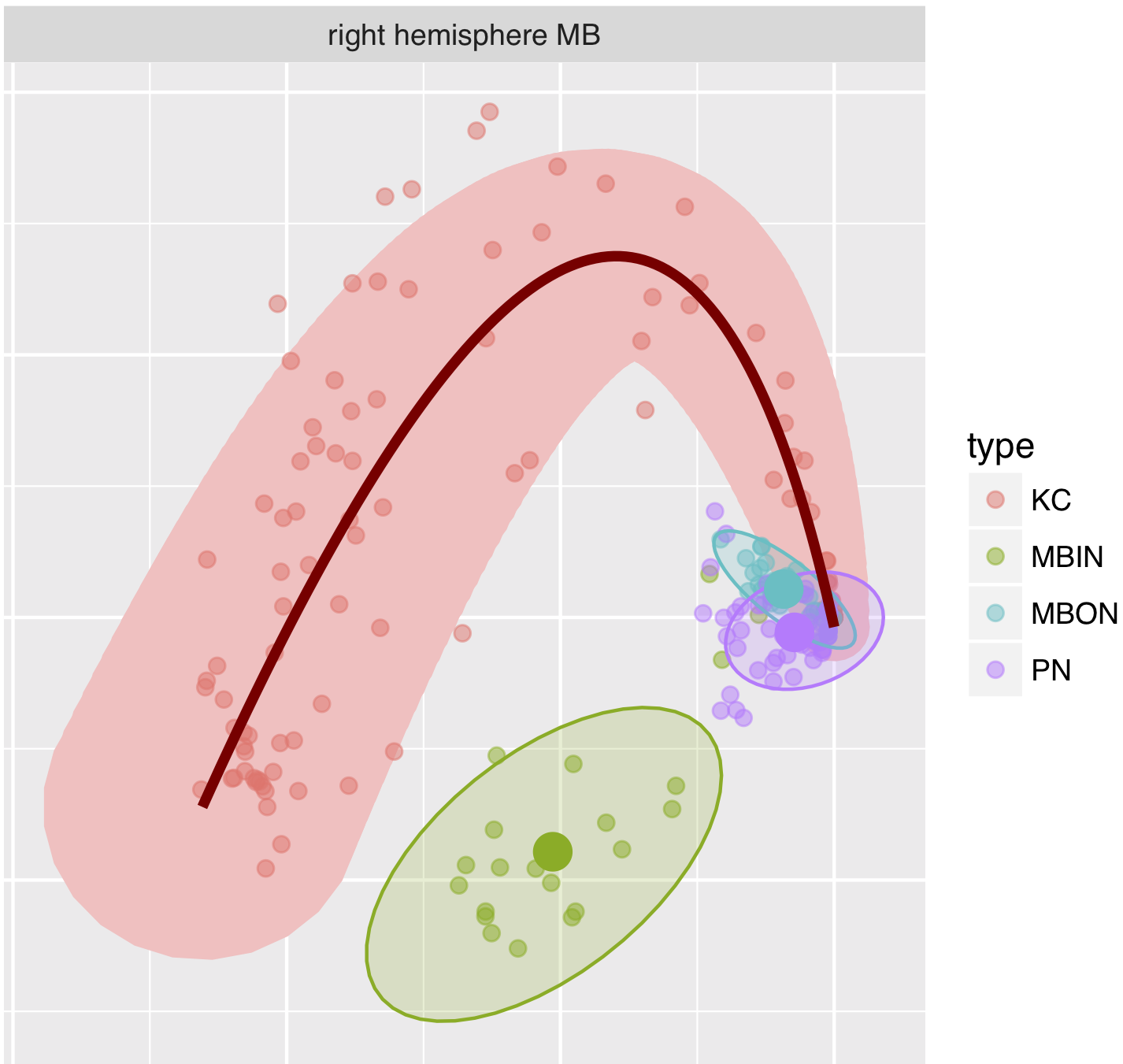
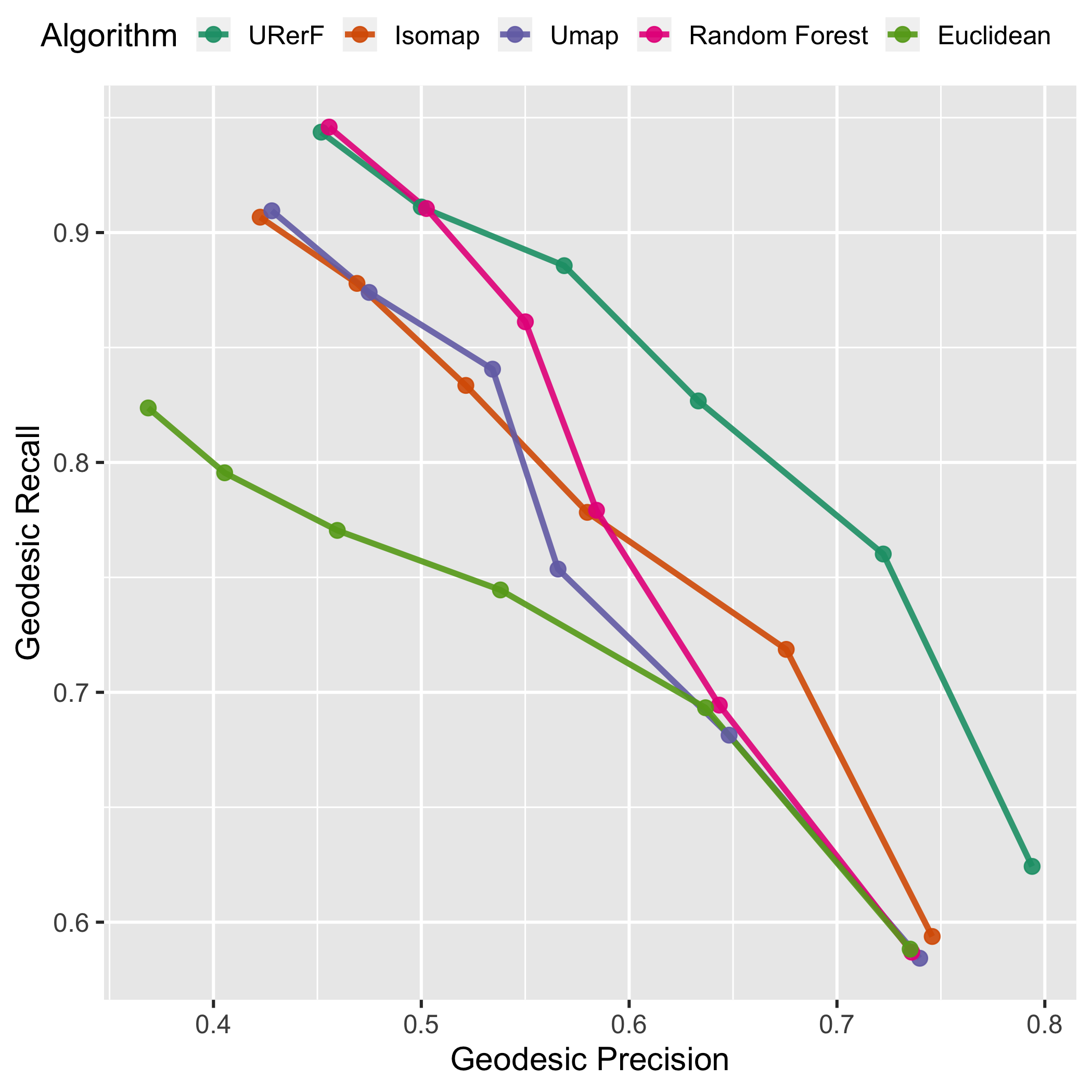
The study of brain networks, or connectomics, is quickly emerging as an important source of real world data challenges [44]. Recently, the entire larval Drosophila mushroom body connectome–the learning and memory system of the fly—was estimated and released [45]. It was obtained via manual labeling and semi-automatic machine vision segmentation of serial section transmission electron microscopy. The 200 nodes of this connectome correspond to 200 distinct neurons in the mushroom body. There are roughly 75000 edges, defined as present between a pair of neurons whenever there exists as least one synapse between them. The edges connect vertices in four known classes of cells: kenyon cells, input neurons, output neurons, and projection neurons [46]. A semiparametric analysis of the connectome, using adjacency spectral embedding [47], results in a six-dimensional latent representation of each node [46]. Because this connectome is directed, the first three dimensions correspond to “outgoing” latent features, whereas the next three correspond to “incoming” latent features. Figure 5 (left) shows two of the six dimensions. Figure 5 on the right shows the geodesic precision versus geodesic recall for various algorithms using cell type as the true label. URerF achieves a higher recall at essentially all precision levels.

Figure 5: Left The right Drosophila connectome after adjacency spectral embedding into six-dimensional space, just showing two of the dimensions. Right Geodesic precision versus geodesic recall for various algorithms using cell type as the true label. URerF achieves a higher recall for essentially all precisions. The values of k for this experiment range from 50 to 250 with increments of 50

Discussion

We proposed a geodesic distance learning method using Unsupervised Randomer Forests (URerF), as well as a splitting rule called Fast-BIC. URerF is empircally robust to noise dimensions, as demonstrated by several different simulation settings, many different added noise dimensions, and the real-world Drosophila connectome. While here we address geodesic learning explicitly, geodesic learning is an essential statistical primitive for many subsequent inference tasks. For example, manifold learning, high-dimensional clustering, anomaly detection, and vertex nomination [48] all rely on geodesic learning. More generally, any ranking problem is essentially a geodesic learning problem. Moreover, while we only considered unsupervised geodesic learning, the ideas presented here immediately lend themselves to supervised geodesic learning as well.

We did not explore any theoretical claims associated with the algorithms presented here. Indeed, we did not even evaluate whether any of these algorithms approximate the precise geodesic. Rather, our metric is concerned purely with getting the geodesic neighbors correct. However, prior work using random projections to learn low-dimensional manifolds [33], and for vector quantization [34], have certain theoretical guarantees associated with the intrinsic dimension of an assumed latent manifold. It seems that those guarantees could relatively easily be transferred to this setting. Another potential direction would be to address the theoretical bounds that geodesic learning can provide with respect to Bayes optimal performance, on both unsupervised and supervised learning problems. For example, 1-nearest neighbor provides tight bounds on Bayes optimal classification [25, 49]. Ideas presented in previous work on bounding Bayes performance using ranking algorithms could also extend to this setting.

URerF is available as part of the open source package “RerF” which includes a Python as well as an R package, available at https://neurodata.io/rerf.

Appendix A Algorithms

Algorithm 1 Build an unsupervised random decision tree. Using sparse linear combinations of features for 1-dimensional projections, find the best splitting point among $d$ of such projections.

1:procedure BuildTree($X,d,\Theta$)

2:Input:

3:$X$ : a subset the of training data of dimension $p$

4:$d$ : dimensionality of the projected space

5:$\Theta$: set of split eligibility criteria Output: a tree t

6:

7:     if $\Theta$ not satisfied then

8:         return LeafNode($X$) $\triangleright$ Create a leaf node

9:     else

10:         $A\leftarrow\left[a_{1}...a_{p}\right]\sim f_{A}$ $\triangleright$ sample random $p\times d$ matrix

11:         $\tilde{X}=A^{T}X$ $\triangleright$ random projection into new feature space

12:         min_t* $\leftarrow\infty$

13:         for  $i\in\{1,...,d\}$ do $\triangleright$ test each projected dimension for optimal split

14:              $\tilde{X}^{(i)}\leftarrow\tilde{X}\left[:,i\right]$

15:              (midpt, t*) = ChooseSplit($\tilde{X}^{(i)}$) $\triangleright$ Use either Algorithm 2 or 3

16:              if  (t* $<$min_t*) then $\triangleright$ store best splitting dimension and split point

17:                  bestDim = i

18:                  splitPoint = midpt

19:              end if

20:         end for

21:         $X_{\textnormal{left}}=\{x\in X|x(\textnormal{bestDim})<\textnormal{splitPoint}\}$

22:         $X_{\textnormal{right}}=\{x\in X|x(\textnormal{bestDim})\geq\textnormal{splitPoint}\}$

23:         Daughters.Left = BuildTree($X_{\textnormal{left}},d,\Theta$)

24:         Daughters.Right = BuildTree($X_{\textnormal{right}},d,\Theta$)

25:         return Daughters

26:     end if

27:end procedure

Algorithm 2 Find the optimal split of one-dimensional data, in terms of the two-means objective.

1:procedure TwoMeans1D($Z$)

2:Input: $Z\in\mathbb{R}^{n}$: set of one-dimensional input values, one per $n$ data points

3:Output: Optimal two-means split point, splitPoint, between points in $Z$ and the corresponding sum of squared distances to the two means, minVars

4:     $\hat{\mu_{1}}\leftarrow\min(Z)$

5:     $\mathcal{C}_{1}\leftarrow\{\hat{\mu}_{1}\}$

6:     $\mathcal{C}_{2}\leftarrow Z\setminus$ $\mathcal{C}_{1}$

7:     $\hat{\mu_{2}}\leftarrow\frac{1}{n_{2}}\sum_{z_{i}\in\mathcal{C}_{2}}z_{i}$ $\triangleright$ mean of $\mathcal{C}_{2}$

8:     vars $\leftarrow\sum_{j=1}^{2}\sum_{z_{i}\in C_{j}}(z_{i}-\mu_{j})^{2}$ $\triangleright$ sum of variances

9:     minVars $\leftarrow$ vars

10:     while  $\mathcal{C}_{2}\neq\emptyset$  do

11:         $z\leftarrow\min(\mathcal{C}_{2})$

12:         $\mathcal{C}_{1}\leftarrow\mathcal{C}_{1}\cup\{z\}$

13:         $\mathcal{C}_{2}\leftarrow\mathcal{C}_{2}\setminus\{z\}$

14:         $\hat{\mu_{1}}\leftarrow\frac{1}{n_{1}}\sum_{z_{i}\in\mathcal{C}_{1}}z_{i}$ $\triangleright$ mean of $\mathcal{C}_{1}$

15:         $\hat{\mu_{2}}\leftarrow\frac{1}{n_{2}}\sum_{z_{i}\in\mathcal{C}_{2}}z_{i}$ $\triangleright$ mean of $\mathcal{C}_{2}$

16:         vars $\leftarrow\sum_{j=1}^{2}\sum_{z_{i}\in\mathcal{C}_{j}}(z_{i}-\mu_{j})^{2}$

17:         if  vars $<$ minVars  then

18:              minVars $\leftarrow$ vars

19:              splitPoint $\leftarrow(\max(\mathcal{C}_{1})+\min(\mathcal{C}_{2}))/2$ $\triangleright$ Midpoint between $\mathcal{C}_{1}$ and $\mathcal{C}_{2}$

20:         end if

21:     end while

22:     return (splitPoint, minVars)

23:end procedure

Algorithm 3 Fast-BIC1D: Find the optimal split, in terms of BIC score, of one-dimensional data with two classes.

1:procedure Fast-BIC1D($Z$)

2:Input: $Z\in\mathbb{R}^{n}$: data matrix containing $n$ points in $1$ dimension

3:Output: (splitPoint, minBIC): The midpoint and estimated BIC score that correspond to the best partition between the points in $Z$

4:     $\hat{\mu}_{1}\leftarrow\min(Z)$

5:     $\mathcal{C}_{1}\leftarrow\{\hat{\mu_{1}}\}$

6:     $\mathcal{C}_{2}\leftarrow Z\setminus$ $\mathcal{C}_{1}$

7:     $\hat{\mu}_{2}\leftarrow\frac{1}{|C_{2}|}\sum_{z_{i}\in\mathcal{C}_{2}}z_{i}$ $\triangleright$ mean of $C_{2}$

8:     BIC_curr $\leftarrow\sum_{j=1}^{2}\sum_{z_{n}\in\mathcal{C}_{j}}(z_{n}-\mu_{j})^{2}$

9:     minBIC_curr $\leftarrow$ dists_sq

10:     while  $\mathcal{C}_{2}\neq\emptyset$  do

11:         $z\leftarrow\min(\mathcal{C}_{2})$

12:         $\mathcal{C}_{1}\leftarrow\mathcal{C}_{1}\cup\{z\}$

13:         $\mathcal{C}_{2}\leftarrow\mathcal{C}_{2}\setminus\{z\}$

14:         for j = 1, 2 do

15:              $n_{j}=|\mathcal{C}_{j}|$

16:              $\hat{w}_{j}=n_{j}/n$

17:              $\hat{\mu_{j}}\leftarrow\frac{1}{n_{j}}\sum_{z_{i}\in\mathcal{C}_{j}}z_{i}$ $\triangleright$ mean of $\mathcal{C}_{j}$

18:              $\hat{\sigma_{j}}^{2}\leftarrow\frac{1}{n_{j}}\sum_{z_{i}\in\mathcal{C}_{j}}(z_{i}-\hat{\mu_{j}})^{2}$ $\triangleright$ variance of $\mathcal{C}_{j}$

19:         end for

20:         $\hat{\sigma}_{\textrm{comb}}^{2}\leftarrow\frac{1}{n}\sum_{j=1}^{2}\sum_{z_{i}\in\mathcal{C}_{j}}(z_{i}-\hat{\mu}_{j})^{2}$

21:         BIC_diff_var $\leftarrow-2(n_{1}\log\hat{w}_{1}-\frac{n_{1}}{2}\log 2\pi\hat{\sigma}_{1}^{2}-n_{2}\log\hat{w}_{2}+\frac{n_{2}}{2}\log 2\pi\hat{\sigma_{2}}^{2})$

22:         BIC_same_var $\leftarrow-2(n_{1}\log\hat{w}_{1}-\frac{n_{1}}{2}\log 2\pi\hat{\sigma}_{\textrm{comb}}^{2}-n_{2}\log\hat{w}_{2}+\frac{n_{2}}{2}\log 2\pi\hat{\sigma}_{\textrm{comb}}^{2})$

23:         BIC_curr $\leftarrow\min$ (BIC_same_var, BIC_diff_var)

24:         if  BIC_curr $<$ minBIC then

25:              minBIC $\leftarrow$ BIC_curr

26:              splitPoint $\leftarrow(\max(\mathcal{C}_{1})+\min(\mathcal{C}_{2}))/2$ $\triangleright$ Midpoint between $\mathcal{C}_{1}$ and $\mathcal{C}_{2}$

27:         end if

28:     end while

29:     return (splitPoint, minBIC)

30:end procedure

Appendix B Simulation Settings

• Linear: each point $x$ is parameterized by $p=(4t,6t,9t)$, with $t\in(0,1)$ where $t$ is sampled from a grid with equal spacing.

• Helix: each point $x$ is parameterized by $p=(t\cos(t),t\sin(t),t)$, with $t\in(2\pi,9\pi)$ on an equally spaced grid.

• Sphere: each point $x$ is parameterized by $p=(r\cos(u)\sin(v),r\sin(u)\sin(v),r\cos(v))$, with $u\in(0,2\pi)$, $v\in(0,\pi)$ and $r=9$ where $u$, $v$ are sampled form a grid with equal spacing.

• Gaussian Mixture: each point $x$ is drawn from a mixture of Gaussian distributions: $\sum\limits_{j=1}^{3}\hat{w}_{j}\mathcal{N}(\mu_{j},\Sigma),$ with $(\pi_{1},\pi_{2},\pi_{3})=(0.3,0.3,0.4)$, $(\hat{\mu_{1}},\hat{\mu_{2}},\mu_{3})=(\begin{bmatrix}-3\\ -3\\ -3\end{bmatrix},\begin{bmatrix}0\\ 0\\ 0\end{bmatrix},\begin{bmatrix}3\\ 3\\ 3\end{bmatrix})$ and $\Sigma=\mathbb{I}$ is the identity matrix.

Appendix C Fast-BIC1D Derivation

The BIC test is an alternative to the two means split criteria. We rank potential splits on the BIC score obtained assuming a model with a mixture of two Gaussians; the elements along a given dimension to the left of the cut point belong to one Gaussian and the elements to the right belong to another Gaussian (the elements are in sorted order). For example, if the elements are [1, 3, 4, 6] along a dimension, possible splits are [[1],[3, 4, 6]] , [[1, 3],[4, 6]] , [[1, 3, 4],[6]]. In the case [[1, 3],[4, 6]], we assume the model to comprise of two Gaussians, where [1,3] are sampled from the first and [4,6] are sampled from the second. We choose the split that results in the lowest BIC score. We then repeat the process for all dimensions and choose the dimension that gives the split resulting in the lowest BIC score. We use the following notation in the below derivation:

• $Z$ : is the set of $n$ points in one-dimension

• $s$ : is the current split point

• $n_{j}$ : Number of elements in cluster $j$

• $w_{j}$ : probability of choosing cluster $j$, $w_{j}=\frac{n_{j}}{n}$

• $\mu_{j}$ : mean of cluster $j$

• $\sigma_{1}^{j}$ : variance of cluster $j$

Computing the log likelihood is slightly different here than for the regular GMM. This is because we already know which element belongs in which cluster, so we can compute the log likelihood directly, without the EM step.

$$\log\ell(Z) =\log\ell(\{z_{n}\}_{n<s})+\log\ell(\{z_{n}\}_{n>s})$$

$$\log\prod_{n}P(x_{n};\mu,\sigma^{2},w) =\sum_{n<s}[\log w_{1}+\log\mathcal{N}(x_{n};\mu_{1},\sigma_{1}^{2}I)]+\sum_{n>s}[\log w_{2}+\log\mathcal{N}(x_{n};\mu_{1},\sigma_{2}^{2}I)]$$ (7)

Substituting the expression for $w_{1}$ and $w_{2}$ and expanding the $\log$ Gaussian, we get the following:

$$\log\prod_{n}P(x_{n};\mu,\sigma^{2},w)=\\ n_{1}\log w_{1}-\frac{n_{1}}{2}\log 2\pi\sigma_{1}^{2}-\sum_{n_{1}}\frac{||x_{n_{1}}-\mu_{1}||^{2}}{2\sigma_{1}^{2}}+n_{2}\log w_{2}-\frac{n_{2}}{2}\log 2\pi\sigma_{2}^{2}-\sum_{n_{2}}\frac{||x_{n_{2}}-\mu_{2}||^{2}}{2\sigma_{2}^{2}}$$ (8)

The parameters $w_{1},w_{2},\mu_{1}$, $\mu_{2}$, $\sigma_{1}$ and $\sigma_{2}$ are unknown. We use the maximum likelihood estimates as a plug-in for each:

$$\hat{w}_{1} =n_{1}/N$$

$$\hat{\mu}_{1} =\frac{1}{n_{1}}\sum_{n<s}x_{n}$$

$$\hat{\sigma_{1}} =\frac{1}{n_{1}}\sum_{n<s}||x_{n}-\hat{\mu}_{1}||^{2},$$

with the parameters for $j=2$ defined equivalently. Thus the right hand side of Equation (8) can be expressed as

$$n_{1}\log w_{1}-\frac{n_{1}}{2}\log 2\pi\hat{\sigma}_{1}^{2}-\frac{n_{1}}{2}+n_{2}\log w_{2}-\frac{n_{2}}{2}\log 2\pi\hat{\sigma}_{2}^{2}-\frac{n_{2}}{2}$$ (9)

But in the BIC formula, we need to compute the negative log likelihood.

$$-\log\prod_{n}P(x_{n};\hat{\mu},\hat{\sigma}^{2},\hat{w})=-n_{1}\log\hat{w}_{1}+\frac{n_{1}}{2}\log 2\pi\hat{\sigma}_{1}^{2}+\frac{n_{1}}{2}-n_{2}\log\hat{w}_{2}+\frac{n_{2}}{2}\log 2\pi\hat{\sigma}_{2}^{2}+\frac{n_{2}}{2}.$$ (10)

Appendix D Supplemental Figures

Figure 6: Geodesic precision at k=50 with varying noise dimension $d^{\prime}$ from 2 to 10, using $N=1000$ samples, and $p=3$ number of non-noisy dimensions. URerF is robust to adding noise dimensions while the other algorithms deteriorate to chance in performance.

References and Notes

- [1] X. Wu, V. Kumar, J. Ross Quinlan, J. Ghosh, Q. Yang, H. Motoda, G. J. McLachlan, A. Ng, B. Liu, P. S. Yu, Z.-H. Zhou, M. Steinbach, D. J. Hand, and D. Steinberg, “Top 10 Algorithms in Data Mining,” Knowledge and information systems, vol. 14, pp. 1–37, Dec. 2007.
- [2] C. J. Stone, “Consistent Nonparametric Regression,” Annals of statistics, vol. 5, pp. 595–620, July 1977.
- [3] L. Breiman, “Random forests,” Machine learning, vol. 45, no. 1, pp. 5–32, 2001.
- [4] Y. Freund and R. E. Schapire, “A decision-theoretic generalization of on-line learning and an application to boosting,” Journal of Computer and System Sciences, 1997.
- [5] R. Caruana and A. Niculescu-Mizil, “An Empirical Comparison of Supervised Learning Algorithms,” in Proceedings of the 23rd International Conference on Machine Learning, ICML ’06, (New York, NY, USA), pp. 161–168, ACM, 2006.
- [6] R. Caruana, N. Karampatziakis, and A. Yessenalina, “An empirical evaluation of supervised learning in high dimensions,” in Proceedings of the 25th international conference on Machine learning, (New York, New York, USA), pp. 96–103, ACM, July 2008.
- [7] T. Chen and C. Guestrin, “XGBoost: A Scalable Tree Boosting System,” in Proceedings of the 22Nd ACM SIGKDD International Conference on Knowledge Discovery and Data Mining, KDD ’16, (New York, NY, USA), pp. 785–794, ACM, 2016.
- [8] M. Aumüller, E. Bernhardsson, and A. Faithfull, “ANN-Benchmarks: A Benchmarking Tool for Approximate Nearest Neighbor Algorithms,” in Similarity Search and Applications, pp. 34–49, Springer International Publishing, 2017.
- [9] B. Schölkopf and A. J. Smola, Learning with kernels: support vector machines, regularization, optimization, and beyond. MIT press, 2002.
- [10] M. Mohri, A. Rostamizadeh, and A. Talwalkar, Foundations of Machine Learning. MIT Press, Nov. 2018.
- [11] W. A. Fuller, Measurement Error Models. Wiley, 99 edition ed., June 1987.
- [12] D. J. Hand, Measurement: A Very Short Introduction (Very Short Introductions). Oxford University Press, 1 edition ed., Dec. 2016.
- [13] J. A. Lee and M. Verleysen, Nonlinear Dimensionality Reduction. Springer Science & Business Media, 2007 edition ed., Dec. 2007.
- [14] W. C. Thibault and B. F. Naylor, “Set operations on polyhedra using binary space partitioning trees,” in ACM SIGGRAPH computer graphics, vol. 21, pp. 153–162, ACM, 1987.
- [15] S. Dasgupta and Y. Freund, “Random projection trees and low dimensional manifolds.,” in STOC, vol. 8, pp. 537–546, Citeseer, 2008.
- [16] L. Breiman, J. Friedman, C. J. Stone, and R. A. Olshen, Classification and Regression Trees (Wadsworth Statistics/Probability). Chapman and Hall/CRC, 1 edition ed., Jan. 1984.
- [17] J. H. Friedman, “Greedy function approximation: a gradient boosting machine,” Annals of statistics, pp. 1189–1232, 2001.
- [18] L. Breiman, “Some infinity theory for predictor ensembles,” tech. rep., Technical Report 579, Statistics Dept. UCB, 2000.
- [19] A. Davies and Z. Ghahramani, “The Random Forest Kernel and other kernels for big data from random partitions,” Feb. 2014.
- [20] E. Scornet, “Random Forests and Kernel Methods,” IEEE Trans. Inf. Theory, vol. 62, pp. 1485–1500, Mar. 2016.
- [21] M. Balog, B. Lakshminarayanan, Z. Ghahramani, D. M. Roy, and Y. W. Teh, “The Mondrian Kernel,” June 2016.
- [22] C. Shen and J. T. Vogelstein, “Decision Forests Induce Characteristic Kernels,” Nov. 2018.
- [23] B. Schölkopf, A. Smola, and K.-R. Müller, “Kernel principal component analysis,” in International Conference on Artificial Neural Networks, pp. 583–588, Springer, 1997.
- [24] T. M. Tomita, M. Maggioni, and J. T. Vogelstein, “Randomer forests,” arXiv preprint arXiv:1506.03410, 2015.
- [25] L. Devroye, L. Györfi, and G. Lugosi, A Probabilistic Theory of Pattern Recognition (Stochastic Modelling and Applied Probability). Springer, corrected edition ed., Feb. 1997.
- [26] J. B. Tenenbaum, V. De Silva, and J. C. Langford, “A global geometric framework for nonlinear dimensionality reduction,” science, vol. 290, no. 5500, pp. 2319–2323, 2000.
- [27] M. Belkin and P. Niyogi, “Laplacian eigenmaps and spectral techniques for embedding and clustering,” in Advances in neural information processing systems, pp. 585–591, 2002.
- [28] L. McInnes and J. Healy, “Umap: Uniform manifold approximation and projection for dimension reduction,” arXiv preprint arXiv:1802.03426, 2018.
- [29] V. D. Silva and J. B. Tenenbaum, “Global Versus Local Methods in Nonlinear Dimensionality Reduction,” in Advances in Neural Information Processing Systems 15 (S. Becker, S. Thrun, and K. Obermayer, eds.), pp. 721–728, MIT Press, 2003.
- [30] L. v. d. Maaten and G. Hinton, “Visualizing Data using t-SNE,” J. Mach. Learn. Res., vol. 9, no. Nov, pp. 2579–2605, 2008.
- [31] L. v. d. Maaten and G. Hinton, “Visualizing data using t-sne,” Journal of machine learning research, vol. 9, no. Nov, pp. 2579–2605, 2008.
- [32] M. Muja and D. G. Lowe, “Scalable nearest neighbor algorithms for high dimensional data,” IEEE Transactions on Pattern Analysis & Machine Intelligence, no. 11, pp. 2227–2240, 2014.
- [33] S. Dasgupta and Y. Freund, “Random projection trees and low dimensional manifolds.,” in STOC, vol. 8, pp. 537–546, Citeseer, 2008.
- [34] S. Dasgupta and Y. Freund, “Random projection trees for vector quantization,” IEEE Trans. Inf. Theory, pp. 3229–3242, May 2008.
- [35] T. Shi and S. Horvath, “Unsupervised learning with random forest predictors,” J. Comput. Graph. Stat., vol. 15, pp. 118–138, Mar. 2006.
- [36] T. Shi and S. Horvath, “Unsupervised learning with random forest predictors,” Journal of Computational and Graphical Statistics, vol. 15, no. 1, pp. 118–138, 2006.
- [37] T. Tomita, M. Maggioni, and J. Vogelstein, “ROFLMAO: Robust Oblique Forests with Linear MAtrix Operations,” in Proceedings of the 2017 SIAM International Conference on Data Mining, Proceedings, pp. 498–506, Society for Industrial and Applied Mathematics, June 2017.
- [38] A. Liaw and M. Wiener, “Classification and regression by randomforest,” R News, vol. 2, no. 3, pp. 18–22, 2002.
- [39] J. H. Ward, “Hierarchical Grouping to Optimize an Objective Function,” Journal of the American Statistical Association, vol. 58, pp. 236–244, Mar. 1963.
- [40] J. A. Hartigan and M. A. Wong, “Algorithm AS 136: A K-Means Clustering Algorithm,” Applied statistics, vol. 28, no. 1, p. 100, 1979.
- [41] D. Arthur and S. Vassilvitskii, “k-means++: The advantages of careful seeding,” in Proceedings of the eighteenth annual ACM-SIAM symposium on Discrete algorithms, pp. 1027–1035, dl.acm.org, 2007.
- [42] C. Fraley and A. E. Raftery, “Model-Based Clustering, Discriminant Analysis, and Density Estimation,” Journal of the American Statistical Association, vol. 97, pp. 611–631, June 2002.
- [43] G. McLachlan and T. Krishnan, The EM Algorithm and Extensions. Wiley-Interscience, 2 edition ed., Mar. 2008.
- [44] J. T. Vogelstein, E. W. Bridgeford, B. D. Pedigo, J. Chung, K. Levin, B. Mensh, and C. E. Priebe, “Connectal coding: discovering the structures linking cognitive phenotypes to individual histories,” Current opinion in neurobiology, vol. 55, pp. 199–212, 2019.
- [45] K. Eichler, F. Li, A. Litwin-Kumar, Y. Park, I. Andrade, C. M. Schneider-Mizell, T. Saumweber, A. Huser, C. Eschbach, B. Gerber, et al., “The complete connectome of a learning and memory centre in an insect brain,” Nature, vol. 548, no. 7666, p. 175, 2017.
- [46] C. E. Priebe, Y. Park, M. Tang, A. Athreya, V. Lyzinski, J. T. Vogelstein, Y. Qin, B. Cocanougher, K. Eichler, M. Zlatic, et al., “Semiparametric spectral modeling of the drosophila connectome,” arXiv preprint arXiv:1705.03297, 2017.
- [47] D. L. Sussman, M. Tang, D. E. Fishkind, and C. E. Priebe, “A consistent adjacency spectral embedding for stochastic blockmodel graphs,” Journal of the American Statistical Association, vol. 107, no. 499, pp. 1119–1128, 2012.
- [48] J. Yoder, L. Chen, H. Pao, E. Bridgeford, K. Levin, D. Fishkind, C. Priebe, and V. Lyzinski, “Vertex nomination: The canonical sampling and the extended spectral nomination schemes,” arXiv preprint arXiv:1802.04960, 2018.
- [49] G. Biau, L. Devroye, and G. Lugosi, “Consistency of random forests and other averaging classifiers,” Journal of Machine Learning Research, vol. 9, no. Sep, pp. 2015–2033, 2008.