Spatio-Temporal Reconstructions of Global CO2-Fluxes using Gaussian Markov Random Fields

Abstract

Atmospheric inverse modelling is a method for reconstructing historical fluxes of green-house gas between land and atmosphere, using observed atmospheric concentrations and an atmospheric tracer transport model. The small number of observed atmospheric concentrations in relation to the number of unknown flux components makes the inverse problem ill-conditioned, and assumptions on the fluxes are needed to constrain the solution. A common practise is to model the fluxes using latent Gaussian fields with a mean structure based on estimated fluxes from combinations of process modelling (natural fluxes) and statistical bookkeeping (anthropogenic emissions). Here, we reconstruct global $\text{CO}_{2}$ flux fields by modelling fluxes using Gaussian Markov Random Fields (GMRF), resulting in a flexible and computational beneficial model with a Matérn-like spatial covariance, and a temporal covariance defined through an auto-regressive model with seasonal dependence.

In contrast to previous inversions, the flux is defined on a spatially continuous domain, and the traditionally discrete flux representation is replaced by integrated fluxes at the resolution specified by the transport model. This formulation removes aggregation errors in the flux covariance, due to the traditional representation of area integrals by fluxes at discrete points, and provides a model closer resembling real-life space-time continuous fluxes.

Key words: Atmospheric inverse modelling, spatio-temporal processes, GMRF, seasonal dependencies

1 Introduction

The steady increase of atmospheric greenhouse gases since the 18${}^{\text{th}}$ century industrial revolution, has been attributed to anthropogenic emissions from mainly fossil fuel burning and land-use changes (Le Quéré et al.,, 2018). In order to limit future global warming associated to increasing greenhouse gas (GHG) concentrations in the atmopshere, we need to better understand the sources and sinks of the GHG fluxes caused by interactions of climate, ecosystems and human activities.

Because direct observations of trace gas fluxes are limited both spatially and in time, the spatio-temporal flux patterns are inferred from mathematical models. Besides bottom up modelling based on prognostic models including process understanding, a top down approach based on observations of atmospheric GHG concentrations is commonly used. Since $\text{CO}_{2}$ is a persistent GHG, the atmosphere itself contains information regarding past fluxes. In combination with models for atmospheric transport, the atmospheric concentrations can be used to reconstruct past fluxes; this is the main idea behind atmospheric inverse modelling (Rayner et al.,, 1999; Enting,, 2002).

The atmospheric concentrations are sampled at several sites across the globe. The high ratio of unknown flux components to observations makes the inversion problem ill-conditioned. Therefore, atmospheric inversion studies have adapted a Bayesian approach by assigning a (Gaussian) prior to the fluxes. The expectation (or prior fluxes) in this prior field combines estimates of natural biosphere fluxes from process-based Dynamical Global Vegetation Model, such as the Biosphere Energy Transfer and Hydrology (BETHY) scheme (Knorr,, 2000) with measurements of ocean fluxes (Takahashi et al.,, 2002, e.g.). Fossil fuel emissions (Boden et al.,, 2011, e.g.) are usually taken as known and are pre-subtracted from the observations.

Many inversion set-ups have been based on low resolution surface fluxes (e.g. at a continental scale), wherein the fluxes have been assumed to be piecewise constant (Gurney et al.,, 2003, 2004; Law et al.,, 2003; Baker et al.,, 2006). This ”big region” approach results in fluxes that are constrained by the observations. However, with a transport model of higher resolution than that of the fluxes, this approach is prone to potential aggregation errors, as well as limited resolution of the estimated posterior fluxes. To overcome these issues, studies like Houweling et al., (1999); Kaminski et al., (1999); Rödenbeck et al., (2003); Michalak et al., (2004); Peters et al., (2005); Zupanski et al., (2007); Mueller et al., (2008), resolved the fluxes at a higher resolution, comparable with that of the transport models. Due to the larger number of unknown fluxes, these ”grid-scale” studies are even more reliant on prior assumptions on the fluxes. Most of the studies assume a Gaussian prior with a priori known dependence structure for the fluxes; Michalak et al., (2004) introduced a geostatistical approach, where unknown parameters in both a regression model for the prior expected fluxes and the spatial dependence structure were inferred from data, thus reducing the extent of prior assumptions. Parallel to the standard inversion techniques, recursive estimation methods, such as Ensemble Kalman Filters (EKF), have been investigated as potential tools for atmospheric inversions (Peters et al.,, 2005; Zupanski et al.,, 2007).

To our knowledge, all previous global inversion studies have used a flux representation defined on a longitude-latitude grid (or at continental scale, Gurney et al.,, 2003, 2004, etc.), with the grid centroids representing flux values. The corresponding covariance is defined based on distances between grid centroids, ignoring the fact that the true underlying flux field is continuous. This discrete representation is especially critical in cases where the grid centroids represent spatial or temporal domains of different sizes, such as the commonly used regular longitude-latitude grids.

In this article we use Gaussian Markov Random Fields (GMRFs) to define a spatially continuous flux model (Section 3). The response from fluxes to observations is obtained by integrating fluxes on a continuous spatial domain (Section 2 and 3.3). Thus, aggregation errors related to the traditional assumption of constant flux within each grid cell are avoided. We use a separable spatio-temporal covariance function, where the temporal dependence in the fluxes is modelled by either an AR(1) or a seasonal AR(12) process (Section 3.2.1). Both temporal dependence structures results in a sparse temporal precision matrix (inverse covariance matrix). The resulting flux model has a sparse spatio-temporal precision matrix on Kronecker form, which enables efficient computations.

Our method is first demonstrated on pseudo data, with atmospheric concentrations simulated from a known flux field (Section 5.2.1). Thereafter, the method is applied to real atmospheric concentration data (Section 5.2.2) to reconstruct the global flux field between 1990 and 2001.

2 Atmospheric inverse modelling

Atmospheric inverse modelling is based on the assumption that the trace gas concentrations can be determined by knowing all source and sink terms as well as the atmospheric transport of the gas. If the trace gas is inert, as $\text{CO}_{2}$, then an observation, $y_{i}=y(\bm{s}_{i},t_{i})$, of atmospheric trace gas concentration at location $\bm{s}_{i}\in S^{2}$ and time $t_{i}\in\mathbb{R}$, can be seen as the contribution from the continuous surface source flux, $f(\bm{s},t)$, integrated with respect to atmospheric transport, $J$, over past time $t\in(-\infty,\,t_{i}]$ and over the Earth’s surfaces $\bm{s}\in$ $S^{2}$:

$$y_{i} =\int_{-\infty}^{t_{i}}\int_{S^{2}}J(\bm{s}_{i},t_{i},\bm{s},t)f(\bm{s},t)d\bm{s}dt+\epsilon_{meas}(\bm{s}_{i},t_{i}).$$ (1)

Here, $J(\bm{s}_{i},t_{i},\bm{s},t)$ quantifies the sensitivity of $y(\bm{s}_{i},t_{i})$ with respect to the flux at spatial location $\bm{s}$ and time $t<t_{i}$, and $\epsilon_{meas}(\bm{s}_{i},t_{i})$ is the measurement error. The interpretation of $J$ is as the atmospheric transport from flux location and time to the observation. After a certain time, $K$, the surface source fluxes are assumed to be well mixed in the atmosphere due to diffusion. Therefore, sensitivities to fluxes at times $t<t_{i}-K$, are equal and given by a constant, $C$. The constant sensitivity to older fluxes allows us to truncate the above time integral at some initial time, $t_{0}$, and replace the response from historical fluxes (fluxes at times $t<t_{0}$) with an initial atmospheric concentration $c_{0}$:

$$y_{i} =c_{0}+C\int_{t_{0}}^{t_{i}-K}\int_{S^{2}}f(\bm{s},t)d\bm{s}dt+\int_{t_{i}-K}^{t_{i}}\int_{S^{2}}J(\bm{s}_{i},t_{i},\bm{s},t)f(\bm{s},t)d\bm{s}dt+\epsilon_{meas}(\bm{s}_{i},t_{i}).$$ (2)

In practise, the sensitivity $J{(\bm{s}_{i},t_{i},\bm{s},t)}$, is not known, and needs to be approximated with a discrete representation using an atmospheric transport model. The result is a transport model, $\bm{J}$, that can be represented by a Jacobian matrix quantifying the sensitivity of observations to discrete fluxes defined on a spatio-temporal grid; the transport grid. In space, this is commonly a regular longitude-latitude grid, whereas in time, the resolution is typical monthly or daily.

Traditionally, the integral over the flux is discretized to the transport grid, with values at grid centroids representing fluxes for the entire grid. The resulting discrete observation model can be presented in matrix form as

$$\bm{y} =c_{0}\cdot\bm{1}+\bm{J}\bm{f}+\bm{\epsilon},$$ (3)

where $c_{0}$ is the atmospheric $\text{CO}_{2}$ -concentration at time $t_{0}$, $\bm{1}$ is a unit vector, and $\bm{J}$ is the transport matrix, providing a linear link between surface fluxes, $\bm{f}$, and observed atmospheric concentrations, $\bm{y}$. A summary of notation can be found in Table 1.

Computational advantages arise by noting that the transport matrix can be divided into two components, $\bm{J}=\begin{bmatrix}\bm{J}_{c}&\bm{J}_{a}\end{bmatrix}$, based on the integral separation in (2). Here, the ”constant” part of the transport matrix, $\bm{J}_{c}$, has a repeating pattern arising from differences in grid cell volumes, whereas the ”active” part of the transport matrix, $\bm{J}_{a}$, has a band structure that contains information on concentration gradients.

The observation errors, $\bm{\epsilon}$, incorporate both measurement errors, $\bm{\epsilon}_{meas}$, and model errors, $\bm{\epsilon}_{mod}$, where the latter are due to imperfections in the atmospheric transport model used to compute sensitivities. Since the system in (3) is typically under-determined, with more unknown flux elements than observations, standard inversion techniques model the fluxes as spatio-temporal Gaussian fields; introducing smoothing restrictions that give an identifiable model. For grid-scale inversions, the fluxes are typically represented as

$$f(\bm{s},t)=\mu(\bm{s},t)+x(\bm{s},t),$$ (4)

with a expectation component, $\mu(\bm{s},t)$, and zero-mean spatio-temporal Gaussian random field, $x(\bm{s},t)$. The expectation component (i.e. prior fluxes) is commonly assumed known and given by a ”best guess”, based on estimates from bottom-up modelling (e.g. Kaminski et al.,, 1999; Rödenbeck et al.,, 2003).

As an alternative approach, Michalak et al., (2004), used a regression model for the expectation, given by

$$\mu(\bm{s},t)=\sum_{j=1}^{p}B_{j}(\bm{s},t)\beta_{j},$$ (5)

where $\{B_{j}\}_{j=1}^{p}$ are known basis functions, and $\{\beta_{j}\}_{j=1}^{p}$ are unknown regression coefficients. In this way, variables believed to scale (linearly) with the $\text{CO}_{2}$ exchange, e.g. population and vegetation, could be included in the model.

The ability to constrain grid-scale inversions depends critically on the assumed spatial and temporal correlations of the fluxes, as modelled by the spatio-temporal random field, $x(\bm{s},t)$. Both Rödenbeck et al., (2003) and Michalak et al., (2004), among others, significantly reduce the flux uncertainties by modelling the spatial dependence using exponential-like covariance functions. A temporal dependence with exponential covariance was introduced by Rödenbeck et al., (2003).

For the ”large-scale” approaches, i.e., constant fluxes at continental scale, the reduction in the number of unknown flux components often results in identifiable models, even without the smoothing constraints of a spatial field. Excluding the field, $x(\bm{s},t)$, from (4), these models reduce to linear regressions, (5), with indicator basis functions that specify the respective regions.

Table 1: Symbols and units (the following dimensions are true for modelling of a single flux field, and will change when both land- and ocean fluxes are modelled).

Symbol	Unit	Dimension	Attribute
$n_{s}$	—	—	$\#$Spatial elements in $\bm{f}$
$n_{t}$	—	—	$\#$Temporal elements in $\bm{f}$ and $\bm{\omega}$
$n_{\ell}$	—	—	$\#$Triangular basis functions
$n_{\text{obs}}$	—	—	Size of $\bm{y}$
$p$	—	—	Size of $\bm{\beta}$
$n_{f}=n_{t}\cdot n_{s}$	—	—	Size of $\bm{f}$
$n_{\omega}=n_{t}\cdot n_{\ell}$	—	—	Size of $\bm{\omega}$
$n_{z}=(n_{t}\cdot n_{\ell})+p$	—	—	Size of $\bm{z}$
$c_{0}$	ppm	$1$	Initial $\text{CO}_{2}$ concentration
$\bm{f}$	kg/grid/year	$n_{f}$	$\text{CO}_{2}$ flux on transport grid
$\bm{\omega}$	kg/$\text{m}^{2}$/year	$n_{\omega}$	Weights (GMRF)
$\bm{\beta}$	—	$p$	Regression coefficients
$\bm{z}$	kg/$\text{m}^{2}$/year	$n=n_{\omega}+p$	Target (GMRF)
$\bm{J}$	ppm/(kg/grid/year)	$n_{\text{obs}}\times n_{f}$	Transport matrix
$\bm{H}$	$\text{m}^{2}$/ grid	$n_{f}\times n$	Integration matrix
$\bm{A}$	ppm/(kg/$\text{m}^{2}$/year)	$n_{\text{obs}}\times n$	Observation matrix

3 Model

The underlying continuous nature of the flux, and the steady increase of observations (see e.g. ICOS,, 2019), makes a continuous representation of the flux field attractive. This would minimize aggregation errors arising from the discrete grid representation, and provide estimates of the flux covariance on a continuous domain. Further a continuous model for fluxes allows the integration in (2) to be performed at different spatial and temporal resolution for different flux components and regoins. This enables the combination of regional and global transport models, while maintaining a consistent definition of the flux covariance structure.

In this paper, the flux model (4) is defined on a spatial continuous domain with discrete temporal resolution, using a Gaussian random field, $x(\bm{s},t)$. For completeness the model presented here allows for both a constant, $\mu_{0}(\bm{s},t)$, and a regression component, $\mu_{\beta}(\bm{s},t)$, in the expectation model, $\mu(\bm{s},t)$. However, in the application we only utilize constant prior fluxes.

3.1 Basis expansion

A Gaussian random field can be specified through its covariance function, ${\text{C}(\bm{s},\bm{s}^{\prime})}$. However, the spatial integration of fluxes in (2) is problematic to compute for such a representation (e.g. Gelfand,, 2010, suggests a solution based on Monte Carlo integration). Instead we model the spatial Gaussian field, in (4), at time $t$ using a basis expansion,

$$x(\bm{s},t)=\sum_{\ell=1}^{n_{\ell}}\phi_{\ell}(\bm{s})\omega_{\ell}(t),$$ (6)

where $\phi_{\ell}(\bm{s})$ are basis functions defined on the sphere, $\omega_{\ell}(t)$ are Gaussian weights, and $n_{\ell}$ is the number of basis functions in the expansion. Stochastic fields represented as in (6) have been introduced before, typical for dimension reduction in applications on big data sets with the aim of reducing computational complexity. Examples include: basis expansion in the spectral domain using spherical harmonics (Lang et al.,, 2015), process convolutions (Higdon,, 2002), and predictive process models (Banerjee et al.,, 2008). Basis functions with compact support have been used to obtain Markov fields that approximate stochastic fields with certain covariance functions (Lindgren and Rue,, 2007; Lindgren et al.,, 2011). Regardless of the choice of basis functions in (6), the spatial integration of the resulting random field, $x(\bm{s},t)$, over a spatial element, $\mathcal{D}$, is given by

$$\int_{\bm{s}\in\mathcal{D}}x(\bm{s},t)ds = \sum_{\ell=1}^{n_{\ell}}\left(\int_{\bm{s}\in\mathcal{D}}\phi_{\ell}(\bm{s})d\bm{s}\right)\omega_{\ell}(t)=\bm{L}\bm{\omega}_{t},$$ (7)

where $\bm{\omega}_{t}=\begin{bmatrix}\omega_{1}(t)&\ldots&\omega_{n_{\ell}}(t)\end{bmatrix}^{T}$ are the weights at time $t$, and the linear operator, $\bm{L}$, has elements given by the integration of the basis functions, $L_{\ell}=\int_{\bm{s}\in\mathcal{D}}\phi_{\ell}(\bm{s})d\bm{s}$. Assuming known basis functions which are independent of model parameters, the elements of $\bm{L}$ can be precomputed (see Appendix B for technical details or e.g. Simpson et al.,, 2016; Moraga et al., 2017a, , for examples of similar approaches).

3.2 Gaussian Markov Random Fields

For the application considered here, the spatial random field, $x(\bm{s},t)$ at time $t$ (4), will be modelled using the stochastic partial differential equation (SPDE) approach with piecewise linear basis functions defined on a Delaunay triangulation (Lindgren et al.,, 2011). Gaussian Markov random fields on irregular grids were first introduced by Lindgren and Rue, (2007) and extended to Markov representations of non-stationary fields by Lindgren et al., (2011) and Bolin et al., (2011). The GMRFs are derived as weak solutions to the SPDE (Whittle,, 1954),

$$(\kappa^{2}-\Delta)^{\alpha/2}\tau x(\bm{s},t)=\mathcal{W}(\bm{s}),$$ (8)

where $\Delta=\sum_{i=1}^{d}\frac{\delta^{2}}{\delta x_{i}^{2}}$ is the Laplacian operator, $\mathcal{W}(\bm{s})$ is a Gaussian white noise process, $\kappa^{2}$ is a range parameter, and $\tau$ is a scaling parameter. The resulting stochastic fields have an approximate Matérn covariance

$$C(x(\bm{0},t),x(\bm{s},t))\propto(\kappa\lVert\bm{s}\rVert)^{\nu}K_{\nu}(\kappa\lVert\bm{s}\rVert),$$

where $\lVert\cdot\rVert$ represents the great circle distance on the sphere, $K_{\nu}$ is the modified Bessel function and $\nu>0$ and $\kappa>0$ are the regularity and range parameters, respectively. Further, $\alpha$ is related to $\nu$ as $\alpha=\nu+d/2$, where $d$ is the dimension of $\bm{s}$. The Matérn covariance family is commonly used for geostatistical data due to its general form (Guttorp and Gneiting,, 2006), and it includes the exponential covariances ($\nu=1/2$) used in previous inversion studies.

Letting $x(\bm{s},t)$ be a zero-mean Gaussian field expressed on the form (6), solving the SPDE (8), with $\alpha=2$, results in the following distribution for the weights, $\omega_{\ell}(t)$,

$$\bm{\omega}_{t} \in N(\bm{0},\bm{Q}_{S}^{-1}), \bm{Q}_{S} =\tau(\kappa^{2}\bm{C}+\bm{G})^{T}\bm{C}^{-1}(\kappa^{2}\bm{C}+\bm{G})\tau,$$ with (9)

where $\bm{Q}_{S}$ is a sparse precision matrix (see Lindgren et al.,, 2011, for details) .

Apart from a few constraints related to numerical stability the locations of the basis functions, and hence the resolution, can be specified freely (Bakka et al.,, 2018). When modelling land and ocean flux separately (see Appendix C), we utilized this freedom by assigning a higher resolution for the domain of interest. The mesh for modelling a single flux field is displayed in Figure 1 (a), whereas for separate flux fields for land and ocean, the meshes are illustrated in Figure 1 (b–c).

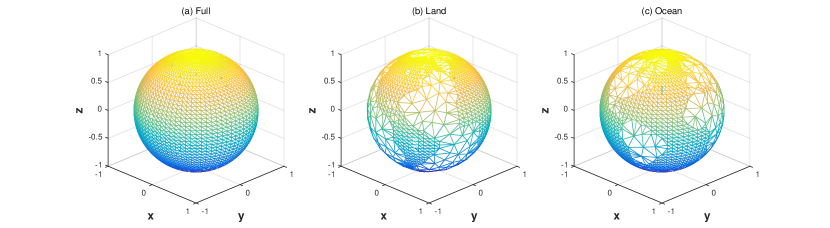
Figure 1: Illustration of triangular basis functions on the sphere when modelling: (a) A single flux field, (b-c) a land and ocean flux field.

3.2.1 Spatio-temporal flux model

The temporal dependence between fluxes is modelled using autoregressive processes. A spatio-temporal field with exponential covariance in time is obtained from a temporal AR(1) process, defined as

$$\bm{\omega}_{t_{m}}=a\bm{\omega}_{t_{m-1}}+\bm{\eta}_{t_{m}}$$ (10)

with spatial dependent driving noise, $\bm{\eta}_{t_{m}}\in N\left(\bm{0},\bm{Q}_{S}\right)$ (Blangiardo and Cameletti,, 2015, Ch. 7). In addition, a seasonal dependence between fluxes is introduced by the following AR(12)-process,

$$\bm{\omega}_{t_{m}}=a\bm{\omega}_{t_{m-1}}+b\bm{\omega}_{t_{m-12}}+\bm{\eta}_{t_{m}}$$ (11)

where $b$ describes the temporal correlation between seasonal fluxes, e.g. January to January. The models described in (10) and (11), together with (9), yield a latent field, $\bm{\omega}=\begin{bmatrix}\bm{\omega}_{t_{1}}^{T}&\ldots&\bm{\omega}_{t_{n_{t}}}^{T}\end{bmatrix}^{T}$, with separable spatio-temporal dependence structure and sparse precision matrix (Blangiardo and Cameletti,, 2015, Ch. 7). The distribution for $\bm{\omega}$ is given by

$$\bm{\omega} \in N(\bm{0},\bm{Q}_{\omega}) \bm{Q}_{\omega} =\bm{Q}_{T}(\bm{\zeta})\otimes\bm{Q}_{S}(\bm{\theta})$$ with (12)

where $\otimes$ is the Kronecker product, $\bm{Q}_{T}$ is the temporal precision matrix from (10) or (11) (see supplementary material for details), $\bm{\zeta}=a$ or $\bm{\zeta}=\begin{bmatrix}a&b\end{bmatrix}$ details the temporal covariance parameters, and $\bm{\theta}=\begin{bmatrix}\tau&\kappa^{2}\end{bmatrix}$ is a vector of spatial covariance parameters.

3.2.2 Marginal flux variance and range

The covariance parameters are often easier to interpret when translated into marginal flux variance, $\sigma^{2}=V(x(\bm{s},t))$, spatial range, $\rho_{S}$, and temporal range, $\rho_{T}$. The spatial marginal variance, $\sigma^{2}_{S}$, is a function of the spatial covariance parameters $\kappa$ and $\tau$, given by

$$\sigma_{S}^{2}=\frac{1}{\tau^{2}}\frac{\Gamma(\nu)}{\Gamma(\nu+d/2)(4\pi)^{d/2}\kappa^{2\nu}}\Biggr{|}_{\begin{subarray}{c}\nu=1\\ d=2\end{subarray}}=\frac{1}{4\pi\tau^{2}\kappa^{2}}.$$ (13)

The temporal marginal covariance, $\sigma^{2}_{T}$, is obtained by solving the Yule-Walker equations (see supplementary material and Ch. 8 in Brockwell,, 2009). Following Lindgren et al., (2011) the range is defined as the spatial/temporal distance at which the correlation is reduced to one tenth. The spatial range for a Matérn covariance with $\nu=1$ is $\rho_{S}=\sqrt{8\nu}/\kappa=\sqrt{8}/\kappa$, the temporal range for an AR(1) process is $\rho_{T}=\log 0.1/\log a$, and for the AR(12) process the range is obtained numerically from the Yule-Walker equations. Note that the spatial distance is defined as the great circles distances divided by the Earth’s radius, and the maximal distance between two locations is $\pi$ (or $180^{\circ}$). The temporal distance is defined in months.

3.3 Flux and observation model

The (numerical) integration of the different flux components (2) to the transport grid can be described by a set of separate linear mappings, which depend on the spatial resolution of the different components; $\bm{L}_{0}$ for the constant expectation component $\mu_{0}(\bm{s},t)$, $\bm{L}_{\beta}$ for the regression component $\mu_{\beta}(\bm{s},t)$, and $\bm{L}_{\omega}$ for the spatially continuous random effect $x(\bm{s},t)$ (see Appendix B for technical details). Resulting in

$$\bm{f}=\bm{L}_{0}\bm{\mu}_{0}+\underbrace{\begin{bmatrix}\bm{L}_{\omega}&\bm{L}_{\beta}\bm{B}\end{bmatrix}}_{\text{$\bm{H}$}}\underbrace{\begin{bmatrix}\bm{\omega}\\ \bm{\beta}\end{bmatrix}}_{\text{$\bm{z}$}},$$ (14)

where $\bm{\mu}_{0}$ and $\bm{B}$ are discrete representations of the constant expectation and regression basis in (5). Assuming a prior Gaussian field for $\bm{w}$, according to (12), and a non-informative Gaussian prior for the regression coefficients $\bm{\beta}$ the joint distribution of the unknown variables, $\bm{z}$, is

$$\bm{z}=\left[\begin{array}[]{c}\bm{\omega}\\ \bm{\beta}\end{array}\right] \in N\left(\left[\begin{array}[]{c}\bm{0}\\ \bm{0}\end{array}\right],{\underbrace{\left[\begin{array}[]{cc}\bm{Q}_{T}(\bm{\zeta})\otimes\bm{Q}_{S}(\bm{\theta})&\bm{0}\\ \bm{0}&\bm{Q}_{\beta}\end{array}\right]}_{\bm{Q}_{z}}}^{-1}\right),$$ (21)

where $\bm{Q}_{\beta}=q_{\beta}\cdot\bm{I}$, and $q_{\beta}$ small (e.g. $q_{\beta}=10^{-4}$). The zero-valued off-diagonal elements in the precision matrix, $\bm{Q}_{z}$, arises from the assumption that $\bm{\omega}$ and $\bm{\beta}$ are a-prior independent.

Combining the observation model (3) with the integration (14) and the flux model defined in (21), we arrive at a conditional observation model

$$\bm{y}|\bm{z} \sim N\left(\bm{y}_{0}+\bm{A}\bm{z},{\bm{Q}_{\epsilon}(\sigma^{2}_{\epsilon})}^{-1}\right),$$ (22)

assuming Gaussian observational error, $\bm{\epsilon}$, with precision matrix $\bm{Q}_{\epsilon}(\sigma^{2}_{\epsilon})$. Here, $\bm{y}_{0}=c_{0}\cdot\bm{1}+\bm{J}\bm{L}_{0}\bm{\mu}_{0}$ is a deterministic expectation term with $c_{0}$ being the initial concentration, and $\bm{J}\bm{L}_{0}\bm{\mu}_{0}$ being the contribution from the fixed expectation. Moreover, $\bm{A}=\bm{J}\bm{H}$ with $\bm{H}$ from (14), is an observation matrix that maps the unknown variables, $\bm{z}$, to the observations, $\bm{y}$, by combining the integration in $\bm{H}$ and the atmospheric transport in $\bm{J}$. Similar to previous inversions, the observation errors, $\bm{\epsilon}$, are assumed to be independent, resulting in an error covariance matrix on the form

$$\bm{Q}_{\epsilon}^{-1}(\sigma^{2}_{\epsilon})=\sigma_{\epsilon}^{2}\bm{M}.$$ (23)

Here, $\bm{M}$ is a diagonal matrix with elements approximating the relative observational variance, and $\sigma_{\epsilon}^{2}$ is an unknown positive scaling constant.

4 Estimation

This model, with a latent Gaussian field (21), and Gaussian observations (22), can be recognized as a standard model in the literature (e.g. Rue and Held,, 2004, p. 39). The posterior distribution of $\bm{z}$ given observations and parameters is

$$\bm{z}|\bm{y}\sim\mathcal{N}(\bm{\mu}_{\bm{z}|\bm{y}}(\bm{\Psi}),{\bm{Q}_{\bm{z}|\bm{y}}(\bm{\Psi})}^{-1}),$$ (24)

where $\bm{\Psi}$ denotes all the (unknown) model parameters, and the posterior expectation and precision are

$$\bm{\mu}_{{\bm{z}}|\bm{y}}(\bm{\Psi}) =\bm{Q}_{\bm{z}|\bm{y}}^{-1}(\bm{\Psi})\bm{A}^{T}\bm{Q}_{\epsilon}(\bm{\Psi})(\bm{y}-\bm{v_{0}})$$ (25)

$$\bm{Q}_{\bm{z}|\bm{y}}(\bm{\Psi}) =\bm{Q}_{\bm{z}}(\bm{\Psi})+\bm{A}^{T}\bm{Q}_{\epsilon}(\bm{\Psi})\bm{A}.$$ (26)

Using (14) posterior estimates and uncertainties for the fluxes are

$$\mathsf{E}(\bm{f}|\bm{y}) =\bm{L}\bm{\mu}_{0}+\bm{H}\bm{\mu}_{{\bm{z}|y}}(\bm{\Psi}),$$ (27)

$$\mathsf{V}(\bm{f}|\bm{y}) =\bm{H}\bm{Q}_{\bm{z}|\bm{y}}^{-1}(\bm{\Psi})\bm{H}^{T}.$$ (28)

The model parameters, $\bm{\Psi}$, are in general unknown, and estimates can be obtained by maximizing the likelihood (see Rue et al.,, 2009, for details)

$$L_{\bm{\Psi}}=p(\bm{y}|\bm{\Psi})=\frac{p(\bm{y}|\bm{z},\bm{\Psi})p(\bm{z}|\bm{\Psi})}{p(\bm{z}|\bm{y},\bm{\Psi})},\quad\forall\bm{z}.$$ (29)

The expression in (29) is valid for any $\bm{z}$, and a standard choice is to evaluate at $\bm{z}=\mu_{\bm{z}|\bm{y}}(\bm{\Psi})$ which reduces the likelihood to

$$L_{\bm{\Psi}}\propto\left(\frac{\lvert\bm{Q}_{\bm{z}}\rvert\lvert\bm{Q}_{{\epsilon}}\rvert}{\lvert\bm{Q}_{\bm{z}|\bm{y}}\rvert}\right)^{1/2}\exp\left(-1/2\left[\bm{\mu}_{\bm{z}|\bm{y}}^{T}\bm{Q}_{\bm{z}}\bm{\mu}_{\bm{z}|\bm{y}}+(\bm{y}-\bm{y}_{0}-\bm{\mu}_{\bm{z}|\bm{y}})^{T}\bm{Q}_{{\epsilon}}(\bm{y}-\bm{y}_{0}-\bm{\mu}_{\bm{z}|\bm{y}})\right]\right).$$ (30)

The posterior density (24) is now obtained by maximizing the likelihood (30), and using the estimated parameter in (25) and (26). Note that $c_{0}$ in the mean component $\bm{y_{0}}$ is unknown, and is here estimated by averaging the first year of measurements after subtracting the response from the prior component, $\bm{J}\bm{L_{0}}\bm{\mu_{0}}$.

4.1 Computational Issues

For point observations of a latent field the observation matrix, $\bm{A}$, will be sparse leading to a sparse posterior precision in (26). Here the inclusion of space-time integration in the observation model (1) leads to a dense observation matrix and dense posterior precision matrix, due to the term $\bm{A}^{T}\bm{Q}_{\epsilon}(\bm{\Psi})\bm{A}$. To avoid the $\mathcal{O}(n^{3})$ computational cost associated with computing the inverses and determinantes of $\bm{Q}_{\bm{z}|\bm{y}}$ in (25) and (30) we simplify the expressions using matrix identities (Harville,, 1997). Details of the simplifications and associated reductions in computational costs can be found in the supplementary material; here we only summarise the results.

The cost of computing $\bm{Q}_{\bm{z}|\bm{y}}^{-1}$ in the posterior expectation (25) can be reduced by applying the Woodbury matrix identity. This leads to a posterior variance expressed through the sparse precision matrices, $\bm{Q}_{\epsilon}^{-1}$ and $\bm{Q}_{z}^{-1}$. The most expensive step when computing the posterior expectation (25) now reduces to solving the equation system

$$\bm{S} =\bm{A}\bm{R}_{z}^{-1}=\bm{J}\bm{H}\bm{R}_{z}^{-1}=\begin{bmatrix}\bm{J}_{c}&\bm{J}_{a}\end{bmatrix}\bm{H}\bm{R}_{z}^{-1}, \bm{Q}_{z} =\bm{R_{z}}^{T}\bm{R_{z}}$$ where (31)

and $\bm{R}_{z}$ is the Cholesky factorization of $\bm{Q}_{z}$. Using the block and Kronecker structure of $\bm{Q}_{z}$ and the division of $\bm{J}$ into constant and active parts the cost of computing $\bm{S}$ is $\mathcal{O}(n_{\text{obs}}n)$ since $\bm{R}_{z}$ is almost as sparse as $\bm{Q}_{z}$ (After reordering $\bm{R}_{z}$ will have $\mathcal{O}(n_{t}n_{\ell}\log n_{\ell})$ non-zero elements, see supplementary material and Rue et al.,, 2009, p. 51.).

The determinants in the likelihood (30) can be simplified (Harville,, 1997, Thm. 8.1) to

$$\frac{\lvert\bm{Q}_{{\bm{z}}}\rvert\lvert\bm{Q}_{\epsilon}\rvert}{\lvert\bm{Q}_{\bm{z}|\bm{y}}\rvert}=\frac{1}{\lvert\bm{Q}_{\epsilon}^{-1}+\bm{S}\bm{S}^{T}\rvert},$$ (32)

where the most expensive calculations is due to the $\mathcal{O}(n_{\text{obs}}^{2}n)$ cost of the $\bm{S}\bm{S}^{T}$-product. Finally we introduce $\bm{L}$ as the following Choleskey factorization

$$\bm{L}^{T}\bm{L} =(\bm{Q}^{-1}_{\epsilon}+\bm{S}\bm{S}^{T}).$$

The resulting simplified posterior expectation and negative log likelihood are:

$$\bm{\mu}_{{z|y}} =\bm{R}_{z}^{-1}(\bm{M}-\bm{S}^{T}\bm{L}^{-1}\bm{L}^{-T}\bm{S}\bm{M})$$ (33)

$$-\log L_{\bm{\Psi}} \propto\log\lvert\bm{L}\rvert+\frac{1}{2}\left(\bm{\mu}_{{z|y}}^{T}\bm{Q}_{\bm{z}}\bm{\mu}_{{z|y}}+(\bm{y}-\bm{y}_{0}-\bm{\mu}_{\bm{z}|\bm{y}})^{T}\bm{Q}_{{\epsilon}}(\bm{y}-\bm{y}_{0}-\bm{\mu}_{\bm{z}|\bm{y}})\right),$$ (34)

where ${\bm{M}=\bm{S}^{T}(\bm{Q}_{\epsilon}(\bm{y}-\bm{y}_{0}))}$.

4.2 Computation of posterior variances

Inverting the posterior precision matrix in (26) to obtain marginal posterior variances for the conditional fluxes (28) is prohibitively expensive. Instead we use a sampling-based approach (Bekas et al.,, 2007), for which the diagonal of a matrix $\bm{B}$, is approximated with the unbiased estimator:

$$\widehat{\text{diag}(\bm{B})}=\bm{U}\odot(\bm{B}\bm{U}).$$ (35)

Here, $\odot$ is the element-wise product, and $\bm{U}$ is a random column vector with elements sampled independently from the Rademacher random numbers; $\mathsf{P}(\bm{U}=\pm 1)=0.5$. Note that the estimate in (35) does not require us to form the complete matrix $\bm{B}$, only the ability to compute $\bm{B}$ multiplied by a vector. Combining (35) and (28) we obtain an estimate of the diagonal elements of the conditional variance, given by:

$$\widehat{\text{diag}(\mathsf{V}(\bm{f}|\bm{y}))}=\bm{U}\odot(\bm{H}\bm{Q}_{{z|y}}^{-1}\bm{H}^{T}\bm{U}).$$ (36)

The uncertainty in the estimator is reduced by averaging over $10\,000$ independent vectors, $\bm{U}$. Again, using the Woodbury matrix identity, we obtained a computationally faster expression,

$$\widehat{\text{diag}(\mathsf{V}(\bm{f}|\bm{y}))}=\bm{U}\odot\left[\bm{H}(\bm{R_{z}}^{-1}(\bm{I}-\bm{S}^{T}\bm{L}^{-1}\bm{L}^{-T}\bm{S})\bm{R_{z}}^{-T}\bm{H}^{T}\bm{U}\right].$$ (37)

Here $\bm{I}$ is the identity matrix, and the matrix products can be evaluated in the computationally most beneficial order.

5 Application

In this section, we apply our method to a real global atmospheric inversion problem. To investigate the full potential of our inversion system, our first analysis is based on simulated $\text{CO}_{2}$ concentrations (at time and locations where we have real data) obtained by running the transport model forward assuming known fluxes (Section 5.2.1). Secondly, using the same inversion system, the posterior fluxes (14) are estimated using real measurements of $\text{CO}_{2}$ concentrations (Section 5.2.2).

In both studies, monthly flux fields of $\text{CO}_{2}$ are estimated for the period 1990 to 2001, using observations of $\text{CO}_{2}$ concentration from 1992 to 2001. Thus, each of the observations will have a model response to at least 25 months of fluxes. The lack of observations in 1990-1991 make the fluxes in this period badly constrained. Therefore, (estimated) posterior fluxes will be analysed for the period 1992 to 2000.

5.1 Data

5.1.1 Observations

The atmospheric CO₂ data are generated according to the procedure described by (Rödenbeck,, 2005) for the Jena Carboscope. It is based on samples collected and analysed by several institutions. Monthly mean values are calculated as the average of the measurements taken within the selected month.

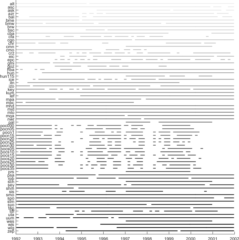
Figure 10: The availability of observations over time for all stations. A more detailed description of the stations can be found in e.g. Rödenbeck, (2005).

The spatial network of $\text{CO}_{2}$ monitoring sites is illustrated in Figure 2. Here, locations indicated with blue triangles are used for estimating the fluxes, while locations marked with red circles are used for validation. The number of available observations at each station varies in time and is shown in Appendix A, Figure 10.

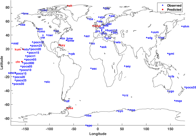
Figure 2: Network of global measurement stations. The observations locations marked with blue triangles are used to estimate fluxes, whereas observation locations indicated with red circles is used for validating the different model performances.

5.1.2 Measurement error

The measurement error is expressed on the form (23), and in the application on real data, the diagonal elements of $\bm{M}$ is defined by

$$M_{ii}=\sigma_{mod,i}^{2}+\sigma_{meas,i}^{2}.$$ (38)

As in Rödenbeck, (2005), the model error, $\sigma_{mod}$, is classified based on the location type, see Table 2. In our study, the measurement error, $\sigma_{meas}$, is set to $0.3$ ppm independently of the number of raw concentration averaged to obtain $y_{i}$. This simplification will have a small effect on the elements of $\bm{M}$, since the model error is much larger than the measurement error. The class specification for the 70 different measurement locations are given in the supplementary material.

Table 2: Class-separated model error that depends on the geographical location as proposed by Rödenbeck, (2005).

Class	Description	$\sigma_{mod}$ (ppm)
C	Continental	3.0
M	Mountain	1.5
R	Remote	1.0
S	Shore	1.5

5.1.3 Transport model

The meteorological transport of fluxes is here approximated by the atmospheric tracer transport model TM3 (Heimann and Körner,, 2003), with a latitude-longitude resolution of approximately $3.8^{\circ}\times 5^{\circ}$, yielding $48\times 72$ rectangular grid cells, and 19 vertical levels. As mentioned before, Jacobian representations of the atmospheric transport model TM3 are used in this study. The monthly Jacobians were calculated by sampling the transport model according to the timing of the actual measurements. The time resolution is one month, and information on gradient concentration range over the last $C=36$ months (2). The sensitivity to fluxes further back in time takes a constant value. As there is no terrestrial productivity on Antarctic and Greenland, the sensitivities to fluxes at these locations are set to zero.

5.1.4 Triangulation

The resolution of the triangulation is similar to the resolution of the TM3 transport grid. The triangulation is obtained by letting the node locations of the basis functions, $s_{\ell}$, be centred in the grid cells of the TM3 model (apart from the grid cells on the poles, where the nodes are located more sparse). This prevents the resolution specified by the triangular nodes to be lower than what can be resolved by the transport matrix. The mesh for modelling a single flux field is shown in Figure 1 (a). When modelling separate land and ocean fields, the flux resolution is higher for the spatial domain of interest, as illustrated in Figure 1 (b–c). Any node included in the mesh for a single flux can be found in either the land or ocean mesh. Moreover, node-points on the boundaries, i.e., node-points centred in TM3 grid cells containing both land and ocean, are included in both the land and ocean triangulations.

5.1.5 Prior fluxes

Prior fluxes consist of three components: net land-atmosphere exchange due to vegetation (Net Ecosystem Exchange, NEE), net ocean-atmosphere exchange (ocean flux), and fossil fuel emissions. All components are resolved on the transport grid (with a spatial resolution of $\approx 4^{\circ}\times 5^{\circ}$). The NEE fluxes consist of monthly NEE simulated from the BETHY dynamic vegetation model (Knorr,, 2000), whereas the ocean fluxes are temporally flat, with spatial ocean fluxes taken from Takahashi et al., (2002). Fossil fuel emission fields are resolved on a monthly time-scale with fossil fields obtained based on linear combinations of the emission fields evaluated at year 1990 (Andres et al.,, 1996) and 1995 (Brenkert,, 2003).

5.2 Models

In total six models (see Table 3) are introduced for modelling the latent field; S0, S1, S12, B0, B1 and B12. The letter S denotes models that include a single flux field, and thus do not separate ocean- and land-flux dynamics. The letter B denotes models that include both land and ocean flux fields (see Appendix C). The model number specifies the order of the autoregressive model used for modelling the time dependence. For example, model S0 models a single flux field assuming temporal independence.

Table 3: Description of the six models used.

Model	Field	AR-order
S0	Single	0
S1	Single	1
S12	Single	12
B0	Separate Land and Ocean	0
B1	Separate Land and Ocean	1
B12	Separate Land and Ocean	12

5.2.1 Simulation study

In the simulation study we only consider a model with zero-mean and a single spatio-temporal random field with seasonal dependence, i.e. model S12. For the simulated observations, two main cases are considered.

In the first case, referred to as bottom-up fluxes, pseudo-observation are based on the prior NEE and ocean fluxes (see Section 5.1.5); excluding the fossil fuel component. The aim of using $\text{CO}_{2}$ observations simulated from the bottom-up fluxes is to investigate the quality of the reconstructions based on known fluxes that resemble real-world $\text{CO}_{2}$ fluxes, and might not follow the Gaussian (and other) assumptions of the model.

In the second case, referred to as the Gaussian fluxes, the known fluxes are obtained by simulating the latent field from the stochastic model S12 using parameters estimated from the prior NEE and ocean fluxes. The aims of using simulated Gaussian fluxes are to evaluate how well model parameters are constrained by the observations and to compare reconstructions obtained with estimated versus true parameters.

In both cases, pseudo-observations are simulated according to (3), with observation error defined on the form (23). Two different noise levels are added; ”low” and ”high”, resulting in four sets of simulated data. The low observation noise has a standard error of $0.1$ ppm ($M_{ii}=0.01$, and $\sigma_{\epsilon}=1$), whereas the the high observational noise has standard deviations in the range 1-3 ppm (with $M$ defined in (38), and $\sigma_{\epsilon}=1$). The ”high” observational noise approximates the variance of the real observations, while the ”low” noise should highlight the reconstruction limits of the transport model.

5.2.2 Real data

The real fluxes are modelled using a deterministic expectation, $\mu_{0}(\bm{s},t)$, and a spatio-temporal field, $x(\bm{s},t)$. The expectation or prior flux, $\mu_{0}$, is constructed by adding up contributions from: 1) a seasonal NEE component obtained by averaging each calender month during 1982–1990; 2) ocean fluxes from Takahashi et al., (2002) which are already averaged in time; and 3) fossil fuel emissions. For the spatio-temporal field all six models in Table 3 are considered.

6 Results

6.1 Simulation study

For the simulation study, parameter estimates are provided in Table 4; root mean square error (RMSE) between the true and posterior flux fields, as well as between predicted and observed $\text{CO}_{2}$ concentrations at the validation sites are given in Table 5; and reconstructed fluxes for the bottom up case are given in Figure 3 (for January, April, July and October of 1999).

For the Gaussian fluxes the estimated parameters are close to those used to generate the data (Tbl. 4); especially for low observational noise. For high observational noise, the estimated range remains close to the true, while the scaling parameter, $\tau$, and the temporal parameters, $a$ and $b$, are slightly shifted. In the case of bottom-up fluxes, the deviations between parameters estimated directly from the fluxes (”true” parameters) and those estimated from $\text{CO}_{2}$ observations are large; we specifically note the shift towards longer spatial range (smaller $\kappa$ values) and stronger seasonal dependence (large $b$) when basing estimates on $\text{CO}_{2}$ observations. These discrepancies might be due to deviations from our Gaussian assumptions. Despite this, the reconstruction errors are of similar magnitude as for the simulated Gaussian fields (Tbl. 5).

Comparing RMSE-values for both $\text{CO}_{2}$ observations at validation sites and the complete flux fields, the errors are comparable between the Gaussian and bottom up data. Recall that the Gaussian fields are simulated using parameters estimated from the bottom up fields and should have comparable variances. Errors increase slightly when using high noise, and for all cases estimated parameters perform as good as or better than known parameters.

The inverse system performs quite well for the low observational noise. Some spatial flux information is lost across the Southern hemisphere and Siberia (Fig. 3); i.e. across regions with few measurement locations (Fig. 2). Using the pseudo-data with the higher noise level, a lot of spatial structure is smoothed out in the reconstructed fluxes, and strong signals in the bottom-up fluxes are only captured when located close to observation sites. However, the posterior fluxes still resolve the large scale patterns of the true fluxes, especially for the Northern hemisphere.

Table 4: Estimated parameter in the simulation study. ”low/high” refers to estimated parameters based on $\text{CO}_{2}$ concentrations observed with low and high noise, respectively. ”True” refers to true parameters, i.e. those estimated from the bottom up flux fields and then used to simulate the Gaussian fluxes. Spatial and temporal range, and standard deviation of the latent field corresponding to the estimated parameters are provided in the lower part of the table.

	True	Bottom up fluxes		Gaussian fluxes
Parameters		Low	High	Low	High
$\sigma_{\epsilon}$	$1.00$	$1.28$	$0.995$	$1.00$	$1.05$
$\tau$	$0.447$	$18.7$	$5.30$	$0.402$	$0.303$
$\kappa$	$23.9$	$3.53$	$5.18$	$22.9$	$23.3$
$a$	$0.555$	$0.0108$	$0.103$	$0.494$	$0.276$
$b$	$0.326$	$0.989$	$0.889$	$0.272$	$0.370$
$\rho_{S}$ – spatial r.	$0.118$	$0.801$	$0.546$	$0.124$	$0.121$
$\rho_{T}$ – temporal r.	$65.0$	$>10^{4}$	$2060$	$27.6$	$25.6$
$\sigma$ – std. dev.	$0.0391$	$0.0734$	$0.0372$	$0.0387$	$0.0458$

Figure 3: Results for the simulation study using observations simulated from the bottom-up fluxes. The first row shows the actual $\text{CO}_{2}$ bottom-up fluxes [$\text{kgC}/(\text{year}\cdot\text{m}^{2})$] for January, April, July, and October of 1999. The second and third row show the resulting posterior fluxes estimated using the S12-model and observations simulated with low and high noise, respectively.

Table 5: RMSE calculated for flux fields and observations (at validation sites) using either true (i.e. estimated directly from the bottom up flux fields or used to simulate the Gaussian fluxes) or estimated (from simulated $\text{CO}_{2}$ observations) model parameters. The results in the first two columns are obtained by simulating observations from bottom-up fluxes, while the results in the last two columns are obtained by simulating Gaussian fluxes. The notation ”low” and ”high” refers to low and high observational noise, respectively.

		Bottom-up fluxes		Gaussian fluxes
	Parameters	Low	High	Low	High
RMSE fluxes ($\text{kgC}/(\text{year}\cdot\text{m}^{2})$)	True	$0.0272$	$0.0319$	$0.0401$	$0.0410$
	Estimated	$0.0245$	$0.0294$	$0.0400$	$0.0410$
RMSE val. data (ppm)	True	$0.245$	$0.508$	$0.518$	$0.579$
	Estimated	$0.143$	$0.406$	$0.511$	$0.568$

6.2 Real data

Model performance for real data was evaluated by computing information criterias, AIC (Akaike,, 1969) and BIC (Schwarz et al.,, 1978), as well as RMSE for the validation data (Tbl. 6). Estimated model parameters for all six models are listed in Table 7.

Table 6: Information criterias (AIC & BIC) and root mean square error (RMSE) calculated for the prior fluxes, and posterior fluxes estimated using the six different models; lower values are better.

Model	AIC	BIC	RMSE (ppm)
$\mu_{0}$			$2.79$
S0	23 819	23 839	$1.40$
S1	22 587	22 614	$1.51$
S12	19 651	19 684	$1.62$
B0	20 896	20 930	$1.33$
B1	19 590	19 636	$1.35$
B12	17 995	18 054	$1.31$

Table 7: The estimated model parameters for all six models are provided in the top part of the table. The bottom part of the table gives the corresponding spatial and temporal ranges, and marginal standard deviations.

Parameter	S0	S1	S12	B0	B1	B12
$\sigma_{\epsilon}$	$1.05$	$0.921$	$0.904$	$0.824$	$0.860$	$0.897$
$\tau_{la}$	$1.31$	$0.265$	$0.285$	$0.007\,05$	$0.0137$	$0.0239$
$\kappa_{la}$	$3.72$	$11.6$	$15.5$	$38.6$	$30.5$	$36.7$
$a_{la}$		$0.782$	$0.269$		$0.618$	$0.149$
$b_{la}$			$0.723$			$0.832$
$\tau_{oc}$				$0.422$	$0.716$	$1.19$
$\kappa_{oc}$				$10.8$	$24.2$	$13.3$
$a_{oc}$					$0.987$	$0.121$
$b_{oc}$						$0.870$
$\rho_{S,la}$ – spatial r.	$0.760$	$0.244$	$0.183$	$0.0733$	$0.0928$	$0.0771$
$\rho_{T,la}$ – temporal r.		$9.36$	$2140$		$4.78$	$767$
$\sigma_{la}$ – std. dev.	$0.0579$	$0.147$	$0.206$	$1.04$	$0.859$	$0.858$
$\rho_{S,oc}$ – spatial r.				$0.262$	$0.117$	$0.213$
$\rho_{T,oc}$ – temporal r.					$176$	$1810$
$\sigma_{oc}$ – std. dev.				$0.0619$	$0.101$	$0.0606$

Including separate models for land and ocean improves performance across all three metrics (AIC, BIC, and RMSE), regardless of the temporal dependence. This is to be expected given the very different dynamics of land and ocean fields; illustrated by the differences in estimated marginal standard deviations, $\sigma_{la}$ and $\sigma_{oc}$, and ranges, $\rho_{la}$ and $\rho_{oc}$. Increasing the temporal structure in the model substantially decreases AIC and BIC for both the single and separate field cases. However, the RMSE values do not follow such a simple pattern. For the models with both land and ocean fields including a seasonal, i.e. AR(12), dependence gives the best result for the validation data, while the models with a single field perform best with no temporal dependence (the RMSE values at each observation and validation site can be found in the supplementary material). Overall the B12 model, land and ocean fields with seasonal dependence, performs best across all metrics.

The improvement from introducing a seasonal dependence is likely due to the strong seasonal trend present in the observational data. In Figure 4, the predicted concentrations at the validation sites based on the B12-model are illustrated together with the observations and the concentrations due to prior fluxes, $\bm{y}_{0}=\bm{c}_{0}+\bm{J}\bm{\mu}_{0}$ in (22). The prior fluxes fail to capture the reduction in $\text{CO}_{2}$ concentrations during summer (June, July, and August), resulting in a strong seasonal component that needs to be modelled by the latent field. We note the generally excellent agreement of the posterior concentrations estimated using the B12 model with the observations, except for some outliers at mainly Mace Head, Ireland (mhd) and Key Biscayne, Florida (key).

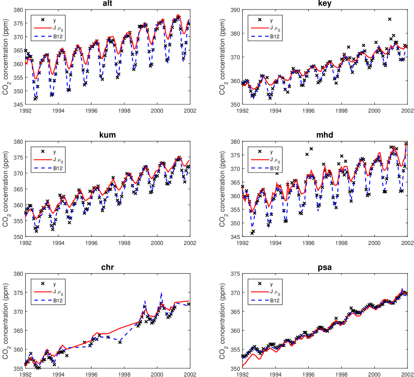
Figure 4: Observed atmospheric $\text{CO}_{2}$ concentrations (black crosses) at the six validation sites (see Fig. 2), illustrated together with predicted concentrations based on the prior fluxes (red solid line) and posterior fluxes (blue dashed line) obtained from the best model: B12.

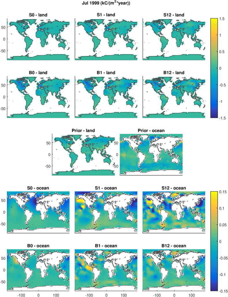
Figure 5: Estimated flux anomalies for July 1999, using the six different models. The first two rows show the land flux anomalies, the third row shows the prior land and ocean fluxes, and the last two rows display the ocean anomalies. Note that the colour scale differs for land and ocean fluxes.

Anomalies for a specific year and month (here July, 1999), estimated using the different models, are shown in Figure 5 (anomalies for January, April and October can be found in the supplementary material). The anomalies were obtained by subtracting the prior flux, $\bm{\mu}_{0}$, from the posterior fluxes (27), and are important for determining which $\text{CO}_{2}$ fluxes that not captured by the prior fluxes. The effect from having separate models for land and ocean fields is clear; resulting in stronger signals over land and weaker signals over oceans. Moreover, having separate land and ocean fields allow us to better resolve fluxes on the Southern continents (South America and Africa). Figure 6 illustrates the approximate posterior standard deviations for the B12-model during July of 1999 obtained using (37). The posterior standard deviations are smaller for areas with many observational sites; e.g. in central Europe and at the west coast of North America. The same holds for the standard deviations of the ocean fluxes, with lower values along the measurement locations in the Pacific Ocean.

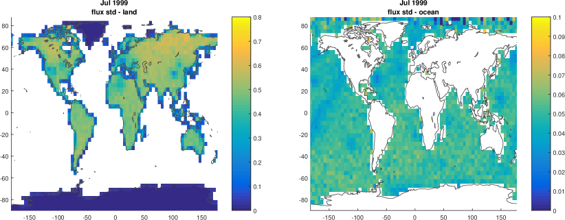
Figure 6: Approximate standard deviations for the land and ocean anomalies estimated using the B12-model (the anomalies are presented in Fig. 5) for July of 1999 [$\text{kgC}/(\text{year}\cdot\text{m}^{2})$].

7 Discussion

7.1 Model parameters

It is interesting to compare the estimated parameters of our best model (Tbl. 7, model B12) with those found in other inversion studies. Firstly, our estimated marginal standard deviations for the land field is about ten times larger than for the ocean field. The higher variability of land fluxes is consistent with previous inversion studies (Mueller et al.,, 2008; Bousquet et al.,, 2000).

For the spatial range most previous studies use an exponential covariance function $r(s)\propto\exp(-s/\ell)$ and report the parameter $\ell$ as the range. The link between $\ell$ and our definition of range is $\rho=\ell\cdot\log(10)$, and all ranges presented here have been transformed to follow our definition and are given in Earth radii. Additionally, previous studies either assume known spatial ranges (Rödenbeck et al.,, 2003) or estimate them from bottom-up fluxes (Mueller et al.,, 2008) and not directly from $\text{CO}_{2}$ observations as done here. Given these caveats, our spatial ranges are much smaller (see Table 8), than those reported in previous studies. However, our final range estimates are consistent with those we obtained from the prior NEE and ocean fluxes using a single field (Bottom-up estimate, Sec. 5.2.1).

Table 8: Comparison of our estimated spatial ranges for the latent flux field, first two lines, with those obtained or used in previous studies. Note that our bottom-up estimate is based on a single field for both land and ocean, and estimated from the prior NEE and ocean fluxes.

	Land	Ocean
Bottom-up estimate	0.118
$\text{CO}_{2}$ observations	$0.0771$	$0.213$
Rödenbeck et al., (2003)	$0.4605$	$0.6908$
Mueller et al., (2008)	$0.9758$	$2.0601$

Both Rödenbeck et al., (2003) and Michalak et al., (2004) use exponential covariances in time, equivalent to an AR(1), with parameters respectively assumed known or estimated from bottom-up fluxes. In contrast Mueller et al., (2008) includes different intercepts for each month in the regression model; essentially creating a seasonal dependence, somewhat similar to our AR(12)-process with $a=0$ and $b=1$. In general, our inclusion of a seasonal AR(12)-process results in substantially larger temporal ranges, than in previous studies.

The strong seasonal component in our model can be motivated by the seasonal trend in the observed $\text{CO}_{2}$ concentrations that is not fully explained by the prior fluxes (Fig. 4). In contrast to the spatial range, the estimated temporal parameters (Tbl. 7) are much larger than those obtained for the prior NEE and ocean fluxes (Tbl. 4), indicating that the temporal dependence might be overestimated. The simulation study also had problems identifying the temporal parameters when using bottom-up flux fields. Theses issues might be due to non-Gaussian distributions of the latent fluxes and/or insufficient information in the inverse system to identify both temporal and spatial dependence. However, despite these problems, models using an AR(12) dependence consistently outperformed all other models both in-sample and for the validation data (Tbl. 6).

7.2 Estimated Posterior fluxes

The reconstructed fluxes averaged across 1996–2000 and divided into prior fluxes, spatial field (anomalies) and posterior fluxes are shown in Figure 7. Two stronger sources in the anomalies are apparent in Northern Germany and South-east Europe (west of the black sea). We suspect, at least for South-east Europe, that this is due to local pollution events from fossil fuel emissions close to the measurement station in this region. In tropical South America we find a dipole source/sink character with the northern part of tropical South America being a source and southern a slight sink of CO₂. The other tropical regions in Africa and Asia are close to neutral or a small source. Note that the tropics, especially in South America, are not well constrained by the observational data due to the location of stations, Fig. 2, and substantial uncertainties in the reconstructions, Fig.6.

In the ocean anomalies, there is a recurrent sink visible in the South Pacific and sources in the North Pacific and in the Norwegian Sea. These patterns are obtained regardless of which model is used to reconstruct fluxes. Remaining sources and sinks have lower amplitudes and are more diffuse.

Average seasonal fluxes are given in Figure 8. Here we can see the large sources in the anomalies in central Europe (mentioned above) but also in the South Eastern USA are mainly apparent in the Northern Hemisphere autumn and winter, i.e. at times when the ecosystem respiration is dominating the terrestrial exchange fluxes. The largest sink occurs in North America and Eurasia during the Northern Hemisphere summer (growing season of the vegetation) and caused by the uptake of $\text{CO}_{2}$ by the vegetation through photosynthesis. For the ocean, there are substantial sinks with a strong seasonality in the North Atlantic and east of Japan in the Pacific.

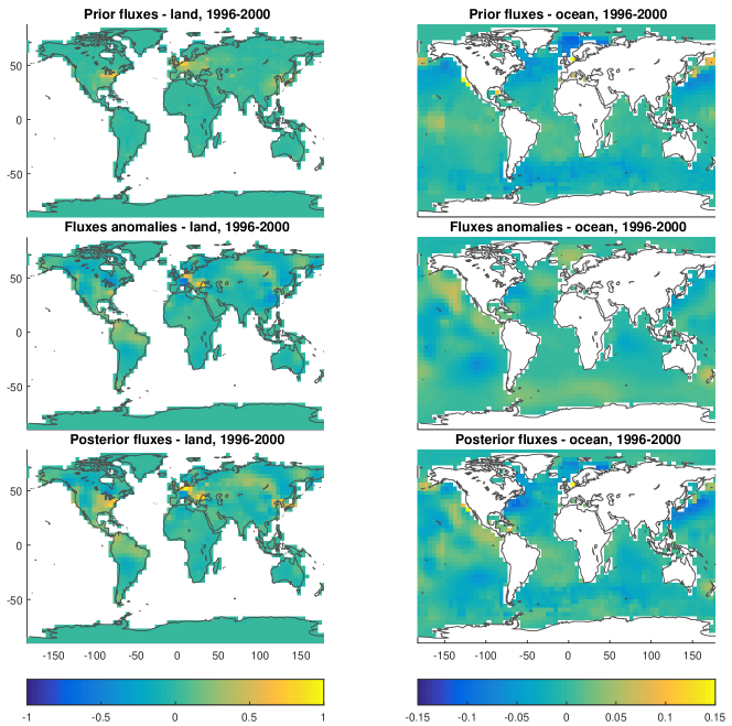
Figure 7: Averaged land and ocean fluxes [$\text{kgC}/(\text{year}\cdot\text{m}^{2})$] over the period 01/1996-12/2000 using the B12-model.

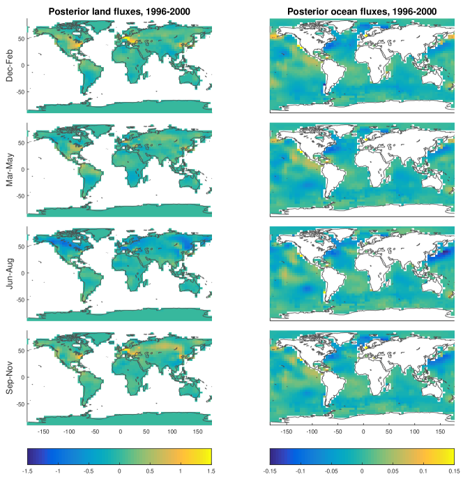
Figure 8: Average seasonal land and ocean fluxes [$\text{kgC}/(\text{year}\cdot\text{m}^{2})$] over the period 01/1996-12/2000 using the B12-model.

7.3 Time series

Time series of reconstructed $\text{CO}_{2}$ fluxes integrated globally and over different regions are shown in Figure 9, for the three models with both land and ocean fields. The contribution due to the fossil component in the prior fluxes, $\bm{\mu}_{0}$, has been removed, and the trends have been deseasonalized by averaging over running yearly intervals.. The regions used correspond to major continental landmasses, tropic and extra-tropical oceans; a map is provided in the supplementary material.

As can be expected, models with more complex temporal dependence, B1 and B12, exhibit smoother temporal trends. The global times-series quite closely resemble those found by Rödenbeck et al., (2003), with increases of $\text{CO}_{2}$ fluxes during 1994–1995 and 1998. When the response is split into land and ocean parts, the main difference with Rödenbeck et al., (2003) is the more distinct ocean peak for 1994–1995 seen in our inversion.

Across the eight individual regions we obtain quite different fluxes, depending on which model is used. The largest differences occur in Tropical and South America, Eurasia, and the Northern Oceans. This suggests that regional fluxes may not be well-constrained by the available observations in these areas, as already mention before in Section 7.2. In fact, the number of stations in these regions is lower than in Europe or North America. The large differences between models for Eurasia and the Northern Ocean are correlated, e.g. the B12-model has the largest sinks over Eurasia and the smallest sinks for the Northern Ocean whereas the opposite is true for the B1-model. We suspect that this is a consequence of the spatial distribution of observations stations across the Northern hemisphere combined with predominant easterly transport due to the dominating westerly wind fields.

Figure 9: Posterior fluxes integrated over different regions and deseasonalized. The top row gives global time-series at a monthly resolution, second row gives the land and ocean contributions, and the remaining rows provide regional fluxes.

8 Conclusion

In this article we introduced a new method for inverse modelling of global $\text{CO}_{2}$ surface fluxes based on GMRFs. In contrast to previous inversion methods, the definition of GMRFs as a basis expansion (6) allows for a spatially continuous representation of the fluxes. The observations response to fluxes is obtained by performing numerical integration over the different flux components, resulting in linear transport matrices. There are three main advantages of this method: (1) The GMRF model on the latent field provides a flexible system for constructing complex spatial and temporal covariances, demonstrated here by the inclusion of seasonal dependences. (2) The flux model represented on a continuous domain better represents the true fluxes, and reduces aggregation errors when combining data at different resolutions (Moraga et al., 2017b, ). (3) Computational advantages obtained through the use of sparse matrices and the Kronecker structure induced by a separable spatio-temporal covariance structure (Rue and Held,, 2004; Bakka et al.,, 2018).

In contrast to previous inversion studies, we estimate all model parameters using observations of $\text{CO}_{2}$ concentrations. Moreover, we show, using a simulation study, that the estimated parameters from $\text{CO}_{2}$ concentrations yield the best flux reconstructions, even when the true parameters of the system are available.

The best flux model obtained in this study, model B12 (see Table 3) has separate fields for land and ocean, and a strong seasonal dependence between months, e.g. January to January. The spatial dependencies in the model is shorter than in previous inversion studies (see Section 7.1). This might be an effect of the stronger temporal dependence combined with an inability of the model to correctly identify both temporal and spatial dependencies due to the limited number of observations.

The GMRF model for fluxes presented here can be extended to non-stationary covariances (Bolin et al.,, 2011; Ingebrigtsen et al.,, 2014). This could account for possible differences in correlation strength due to e.g. latitude (different vegetation, climate zones and dominating wind directions) and land/ocean interactions. However, more unknown parameters, would require more data to constrain, and we have therefore limited this study to stationary covariance models. With increasing measurements from satellites such as NASA’s Orbiting Carbon Observatory-2 (OCO-2,, 2019) the extension to a non-stationary covariance models could be interesting.

Additional information and supporting material for this article is available online at the journal’s website.

Appendix A Additional material

Appendix B Discretization

To compute the relation between latent flux fields and observations we need to evaluate the integral over space and time in (1). Introducing an initial $\text{CO}_{2}$ concentration, $c_{0}$, and truncating the temporal integral reduces (1) to (2). In practice the transport or sensitivity, $\bm{J}$, is defined at some spatial resolution (often a grid) on the globe, $\mathcal{J}=\{s_{k}\}_{k=1}^{n_{s}}$, and for regular time points $\{t_{m}\}_{m=1}^{n_{t}}$, where $n_{s}$ and $n_{t}$ are the spatial and temporal resolutions, respectively. Given a discrete representation of the sensitivity, i.e. $J(s_{i},t_{i},s_{k},t_{m})$, the spatially continuous observation model in (2) can be written as

$$\begin{split}y(s_{i},t_{i})&=c_{0}+\sum_{m=1}^{n_{t}}\sum_{k=1}^{n_{s}}J(s_{i},t_{i},s_{k},t_{m})\int_{\bm{s}\in s_{k}}\!\!f(\bm{s},t_{m})d\bm{s}+\epsilon(\bm{s},t)\\ &=c_{0}+\sum_{m=1}^{n_{t}}\sum_{k=1}^{n_{s}}J(s_{i},t_{i},s_{k},t_{m})\int_{\bm{s}\in s_{k}}\!\!\biggl{(}\mu_{0}(\bm{s},t_{m})+\mu_{\beta}(\bm{s},t_{m})+\sum_{\ell=1}^{n_{\ell}}\phi_{\ell}(\bm{s})\omega_{\ell}(t)\biggr{)}d\bm{s}+\epsilon(\bm{s},t),\end{split}$$

where $s_{k}$ should be interpreted as a grid cell. Here, we have allowed for a flux field consisting of a stochastic spatial field given by a basis expansion, as in (6), as well as a mean given by a constant and a regression component, see (14). The flux components ($\mu_{0}(\bm{s},t)$, $\mu_{\beta}(\bm{s},t)$, and $x(\bm{s},t)$) might be provided at resolutions that differ from the transport resolution, in which case they need to be integrated over the spatial domain specified by $\mathcal{J}=\{s_{k}\}_{k=1}^{n_{s}}$. Numerical integration of the flux components can be performed by forming matrices, $\bm{L}_{0}$, $\bm{L}_{\beta}$ and $\bm{L}_{\omega}$, that map each component to the transport grid.

B.1 Discretization of mean components

Let, $\bm{\mu}_{0}^{(\mathcal{U})}(s_{u},t_{m})$, be a discrete spatial representation of the constant mean at time $t_{m}$, given at a spatial resolution of $\mathcal{U}=\{s_{u}\}_{u=1}^{n_{u}}$ (again $s_{u}$ is a grid cell). The corresponding constant mean defined on the same resolution as the transport grid is given by

$$\bm{\mu}_{0}^{(\mathcal{J})}(s_{k},t_{m})=\!\!\!\int\limits_{\bm{s}\in s_{k}}\!\!\!\mu_{0}(\bm{s},t_{m})\,d\bm{s}\approx\sum_{u=1}^{n_{u}}\bm{\mu}_{0}^{(\mathcal{U})}(s_{u},t_{m})\!\!\!\!\!\!\int\limits_{\bm{s}\in s_{k}\cap s_{u}}\!\!\!\!\!\!1\,d\bm{s}=\sum_{u=1}^{n_{u}}D^{(\mathcal{U},\mathcal{J})}_{ku}\bm{\mu}_{0}^{(\mathcal{U})}(s_{u},t_{m}),$$

where the spatial mapping at time $t_{m}$ is given by a matrix with elements equal to the area of overlap between grid cells in the two spatial resolutions:

$$D^{(\mathcal{U},\mathcal{J})}_{ku}\triangleq\lvert s_{k}\cap s_{u}\rvert.$$ (39)

Since the spatial integration defined by (39) is independent of time the mapping between the spatio-temporal components, $\bm{\mu}_{0}^{(\mathcal{U})}$ and $\bm{\mu}_{0}^{(\mathcal{J})}$, can be formed by a tensor product

$$\bm{L}_{0}=\bm{I}_{n_{t}}\otimes\bm{D}^{(\mathcal{U},\mathcal{J})},$$ (40)

where $\bm{I}_{n_{t}}$ is an identity matrix of size $n_{t}$. Similarly, the basis functions used in the regression mean, e.g. $B_{j}(\bm{s},t)$ in (5), are mapped to the transport grid using

$$\bm{L}_{\beta} =\bm{I}_{n_{t}}\otimes\bm{D}^{(\mathcal{V},\mathcal{J})} D^{(\mathcal{V},\mathcal{J})}_{kv} \triangleq\lvert s_{k}\cap s_{v}\rvert,$$ with elements (41)

where $\mathcal{V}=\{s_{v}\}_{v=1}^{n_{v}}$ is the resolution at which covariates are provided. If the constant mean and/or covariates are provided at the same resolution as the transport matrix — i.e. if $\mathcal{U}$ and/or $\mathcal{V}$ are equal to $\mathcal{J}$ — the corresponding matrices, $\bm{L}_{0}$ and/or $\bm{L}_{\beta}$, simplify to identity matrices of suitable size.

B.2 Discretization of the stochastic field

For the spatial field the integration over $\mathcal{J}$ is performed numerically. First we define a (very) dense grid with centre points $s_{i}$ (see Figure 11) for each grid cell $s_{k}$ in $\mathcal{J}$. Given a basis expansion (6) of the spatial field, the basis functions are evaluated for each point in the dense grid, and the integrals are approximated using sums,

$$\int_{\bm{s}\in s_{k}}\!\!\!\!x(\bm{s},t)d\bm{s} =\sum_{\ell=1}^{n_{\ell}}\left(\int_{\bm{s}\in s_{k}}\!\!\!\!\phi_{\ell}(\bm{s})d\bm{s}\right)\omega_{\ell}(t)\approx\sum_{\ell=1}^{n_{\ell}}\left(\sum_{\{i:s_{i}\in s_{k}\}}\!\!\!\phi_{\ell}(s_{i})\Delta s_{i}\right)\omega_{\ell}(t).$$ (42)

Here $\Delta s_{i}$ represents the size of the grid cell centred at $s_{i}$; note that the grid cells will be of unequal size since the grid is defined on a sphere.

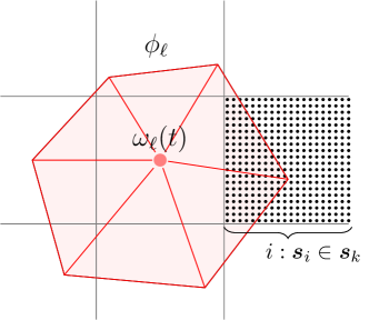
Figure 11: The numerical integration of basis functions to the observation grid, $s_{k}\in\mathcal{J}$, is done by evaluating the basis functions across a very dense grid, $s_{i}$, and replacing integrals by the corresponding approximate sums over $i$.

Introducing a matrix $\bm{G}$ with elements

$$G_{k\ell}\triangleq\sum_{\{i:s_{i}\in s_{k}\}}\!\!\!\phi_{\ell}(s_{i})\Delta s_{i},$$ (43)

and following the same argument regarding repeated temporal fields as in (40), the mapping from the weights in the spatio-temporal random field, $\bm{\omega}$, to the transport grid will be given by $\bm{L_{\omega}}=\bm{I}_{n_{t}}\otimes\bm{G}$.

Combining the spatio-temporal integration of all components, a discretized version of the transport model in (2) can be written as,

$$\begin{split}\bm{y}&=c_{0}\cdot\bm{1}+\bm{J}\bm{L}_{0}\bm{\mu}_{0}+\bm{J}\bm{L}_{\beta}\bm{B}\bm{\beta}+\bm{J}\bm{L}_{\omega}\bm{\omega}+\bm{\epsilon}\\ &=\underbrace{c_{0}\cdot\bm{1}+\bm{J}\bm{L}_{0}\bm{\mu}_{0}}_{\bm{y}_{0}}+\bm{J}\underbrace{\begin{bmatrix}\bm{L}_{\omega}&\bm{L}_{\beta}\bm{B}\end{bmatrix}}_{\bm{H}}\underbrace{\begin{bmatrix}\bm{\omega}\\ \bm{\beta}\end{bmatrix}}_{\bm{z}}+\bm{\epsilon},\end{split}$$

which results in the observation model in (14) and (22).

Appendix C Model Extension

Different dynamics for continental and ocean fluxes can be obtained by using separate flux models for land and ocean. With the latent field taking the land flux value if $\bm{s}$ is over land and the ocean flux value otherwise, we obtain a spatio-temporal flux model given by

$$f(\bm{s},t)=\mathbb{I}_{la}(\bm{s})f_{la}(\bm{s},t)+\mathbb{I}_{oc}(\bm{s})f_{oc}(t,\bm{s}).$$ (44)

where, $\mathbb{I}_{la}$ and $\mathbb{I}_{oc}$ are indicator functions defined as

$$\mathbb{I}_{la}(\bm{s}) =\begin{cases}1,&\text{if $\bm{s}\in$ land,}\\ 0,&\text{if $\bm{s}\in$ ocean,}\end{cases} \mathbb{I}_{oc}(\bm{s}) =\begin{cases}0,&\text{if $\bm{s}\in$ land,}\\ 1,&\text{if $\bm{s}\in$ ocean.}\end{cases}$$

As before the individual fluxes, $f_{la}(\bm{s},t)$ and $f_{oc}(\bm{s},t)$, are represented on the form (21); now with separate mean models and spatio-temporal dependencies. The full flux model, cf. (14), becomes

$$\bm{f} =\bm{L}_{0}\bm{\mu}_{0}+\underbrace{\begin{bmatrix}\bm{L}_{\omega_{la}}&\bm{L}_{\omega_{oc}}&\bm{L}_{\beta_{la}}\bm{B}&\bm{L}_{\beta_{oc}}\bm{B}\end{bmatrix}}_{\bm{H}}\underbrace{\begin{bmatrix}\bm{\omega}_{la}\\ \bm{\omega}_{oc}\\ \bm{\beta}_{la}\\ \bm{\beta}_{oc}\end{bmatrix}}_{\bm{z}},$$ (45)

where the $\bm{L}$ matrices are computed by accounting for the land/ocean indicators in the numerical integration detailed in Section 3.3 and Appendix B. Assuming prior uncorrelated land and ocean fluxes, the distribution for the latent $\bm{z}$-field is

$$\bm{z}=\begin{bmatrix}\bm{\omega}_{la}\\ \bm{\omega}_{oc}\\ \bm{\beta}_{la}\\ \bm{\beta}_{oc}\end{bmatrix} \in N\left(\begin{bmatrix}\bm{0}\\ \bm{0}\\ \bm{0}\\ \bm{0}\end{bmatrix},\begin{bmatrix}\bm{Q}_{T}(a_{la})\otimes\bm{Q}_{S}(\bm{\theta}_{la})&\bm{0}&\bm{0}&\bm{0}\\ \bm{0}&\bm{Q}_{T}(a_{oc})\otimes\bm{Q}_{S}(\bm{\theta}_{oc})&\bm{0}&\bm{0}\\ \bm{0}&\bm{0}&\bm{Q}_{\beta_{la}}&\bm{0}\\ \bm{0}&\bm{0}&\bm{0}&\bm{Q}_{\beta_{oc}}\end{bmatrix}\right).$$ (46)

Supplementary Material

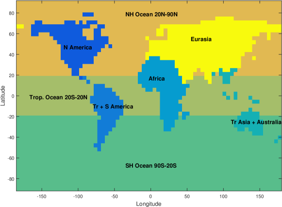
Figure 14: Earth divided into eight regions, five continental regions and three ocean regions, for analysis of regional trends in $\text{CO}_{2}$ .

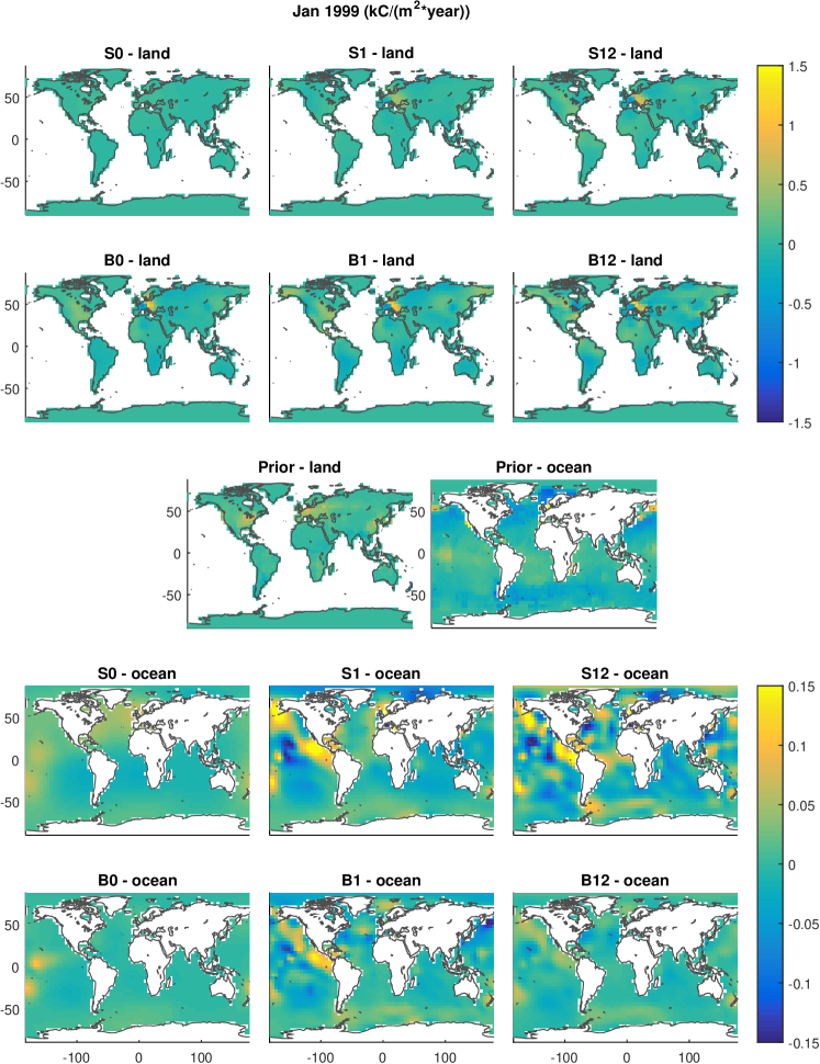
Figure 15: Flux anomalies for January 1999, using the six different models. The first two rows show the estimated land flux anomalies, the third row shows the prior mean land and ocean fluxes, and the last two rows display the estimated ocean anomalies. Note that the colour scale differs for land and ocean fluxes.

This supplementary material to the article Spatio-Temporal Reconstructions of Global CO2-Fluxes using Gaussian Markov Random Fields provides some additional technical details and results not included in the main paper. The precision matrix for a seasonal AR(12)-process and the Yule-Walker equations for computing corresponding covariance functions are provided in Section S1. Section S2 provides details of the likelihood simplifications using the Woodbury, (1950) matrix identity and resulting computational complexities. Finally, Section S3 provides additional figures and results. This includes: The class specification and reconstruction error at the 70 measurement locations (Tbl. LABEL:tab:bias_rmse_class); the division of earth into regions used in the analysis of regional trends (Fig. 14); and flux anomalies for January, April and October of 1999 using all 6 models in Figures 15—17.

Appendix S1 Temporal precision matrix

The temporal dependence in our model is obtained by driving an AR(1) or a seasonal AR(12) process with spatially dependent noise. The precision matrix for the resulting spatio-temporal process is given by the Kronecker product between the precision for the AR-process and the driving noise (Blangiardo and Cameletti,, 2015, Ch. 7): $\bm{Q}_{\omega}=\bm{Q}_{T}\otimes\bm{Q}_{S}$.

To determine the temporal precision we consider a seasonal AR(p) process with

$$x_{t} =ax_{t-1}+bx_{t-p}+\eta_{t}, \eta_{t}\sim N(0,\sigma^{2}).$$ (47)

The conditional distribution is given by

$$[x_{t}|x_{-t}] =[x_{t}|x_{t-1},x_{t-p}]\in N(ax_{t-1}+bx_{t-p},\sigma_{e}^{2}),\qquad t>p>1,$$ (48)

where $x_{-t}$ contains all elements occurring before $t$, i.e. $x_{-t}=\{x_{\tau}:t>\tau\geq 1\}$. The distribution for the vector $\bm{x}=\begin{bmatrix}x_{T}&x_{T-1}&\ldots&x_{1}\end{bmatrix}$ can be written as a product of conditional distributions and an initial stationary component:

$$\begin{split}p(\bm{x})=&\left(\prod_{t=p+1}^{T}p(x_{t}|x_{t-1},x_{t-p})\right)p(x_{p},\ldots,x_{1})\propto\\ \propto&\exp\left(-\frac{1}{\sigma^{2}}\sum_{t=p+1}^{T}{(x_{t}-ax_{t-1}-bx_{t-p})}^{2}\right)p(x_{p},\ldots,x_{1})=\\ =&\exp\left(-\frac{1}{\sigma^{2}}\bm{x}^{T}\bm{Q}_{T}\bm{x}\right),\end{split}$$ (49)

where we want to identify the (scaled) precision matrix, $\bm{Q}_{T}$. The quadratic sum above expands to

$$\begin{split}\sum_{t=p+1}^{T}{(x_{t}-ax_{t-1}-bx_{t-p})}^{2}=&\sum_{t=p+1}^{T}x_{t}^{2}+\sum_{t=p}^{T-1}a^{2}x_{t}^{2}+\sum_{t=1}^{T-p}b^{2}x_{t}^{2}-\sum_{t=p+1}^{T}2ax_{t}x_{t-1}+\\ &+\sum_{t=p+1}^{T}2bx_{t}x_{t-p}+\sum_{t=p+1}^{T}2abx_{t-1}x_{t-p}.\end{split}$$ (50)

Given a stationary initial distribution for $p(x_{p},\ldots,x_{1})$ the final elements of the time-series will be stationary, and by symmetry the top left and lower left corner of a stationary precision matrix $\bm{Q}_{T}$ have to be equal. Identifying the elements in (50) with corresponding elements in the quadratic form $\bm{x}^{T}\bm{Q}_{T}\bm{x}$ the temporal precision matrix is:

$$\bm{Q}_{T}=\hbox{}\vbox{\kern 0.86108pt\hbox{$\kern 0.0pt\kern 2.5pt\kern-5.0pt\left[\kern 0.0pt\kern-2.5pt\kern-5.55557pt\vbox{\kern-0.86108pt\vbox{\vbox{ \halign{\kern\arraycolsep\hfil\@arstrut$\kbcolstyle#$\hfil\kern\arraycolsep& \kern\arraycolsep\hfil$\@kbrowstyle#$\ifkbalignright\relax\else\hfil\fi\kern\arraycolsep&& \kern\arraycolsep\hfil$\@kbrowstyle#$\ifkbalignright\relax\else\hfil\fi\kern\arraycolsep\cr 5.0pt\hfil\@arstrut$\scriptstyle\mbox{indices}$\hfil\kern 5.0pt&5.0pt\hfil$\scriptstyle 1$\hfil\kern 5.0pt&5.0pt\hfil$\scriptstyle 2$\hfil\kern 5.0pt&5.0pt\hfil$\scriptstyle 3$\hfil\kern 5.0pt&5.0pt\hfil$\scriptstyle\ldots$\hfil\kern 5.0pt&5.0pt\hfil$\scriptstyle p$\hfil\kern 5.0pt&5.0pt\hfil$\scriptstyle p+1$\hfil\kern 5.0pt&5.0pt\hfil$\scriptstyle p+2$\hfil\kern 5.0pt&5.0pt\hfil$\scriptstyle\ldots\\1$\hfil\kern 5.0pt&5.0pt\hfil$\scriptstyle 1$\hfil\kern 5.0pt&5.0pt\hfil$\scriptstyle-a$\hfil\kern 5.0pt&5.0pt\hfil$\scriptstyle$\hfil\kern 5.0pt&5.0pt\hfil$\scriptstyle$\hfil\kern 5.0pt&5.0pt\hfil$\scriptstyle 0$\hfil\kern 5.0pt&5.0pt\hfil$\scriptstyle-b$\hfil\kern 5.0pt&5.0pt\hfil$\scriptstyle$\hfil\kern 5.0pt&5.0pt\hfil$\scriptstyle\\2$\hfil\kern 5.0pt&5.0pt\hfil$\scriptstyle-a$\hfil\kern 5.0pt&5.0pt\hfil$\scriptstyle 1+a^{2}$\hfil\kern 5.0pt&5.0pt\hfil$\scriptstyle-a$\hfil\kern 5.0pt&5.0pt\hfil$\scriptstyle$\hfil\kern 5.0pt&5.0pt\hfil$\scriptstyle$\hfil\kern 5.0pt&5.0pt\hfil$\scriptstyle ab$\hfil\kern 5.0pt&5.0pt\hfil$\scriptstyle-b$\hfil\kern 5.0pt&5.0pt\hfil$\scriptstyle\\3$\hfil\kern 5.0pt&5.0pt\hfil$\scriptstyle$\hfil\kern 5.0pt&5.0pt\hfil$\scriptstyle-a$\hfil\kern 5.0pt&5.0pt\hfil$\scriptstyle 1+a^{2}$\hfil\kern 5.0pt&5.0pt\hfil$\scriptstyle-a$\hfil\kern 5.0pt&5.0pt\hfil$\scriptstyle$\hfil\kern 5.0pt&5.0pt\hfil$\scriptstyle$\hfil\kern 5.0pt&5.0pt\hfil$\scriptstyle ab$\hfil\kern 5.0pt&5.0pt\hfil$\scriptstyle\ddots$\hfil\kern 5.0pt&5.0pt\hfil$\scriptstyle$\hfil\kern 5.0pt&5.0pt\hfil$\scriptstyle\\\vdots$\hfil\kern 5.0pt&5.0pt\hfil$\scriptstyle$\hfil\kern 5.0pt&5.0pt\hfil$\scriptstyle$\hfil\kern 5.0pt&5.0pt\hfil$\scriptstyle$\hfil\kern 5.0pt&5.0pt\hfil$\scriptstyle\ddots$\hfil\kern 5.0pt&5.0pt\hfil$\scriptstyle$\hfil\kern 5.0pt&5.0pt\hfil$\scriptstyle$\hfil\kern 5.0pt&5.0pt\hfil$\scriptstyle$\hfil\kern 5.0pt&5.0pt\hfil$\scriptstyle\\p$\hfil\kern 5.0pt&5.0pt\hfil$\scriptstyle 0$\hfil\kern 5.0pt&5.0pt\hfil$\scriptstyle$\hfil\kern 5.0pt&5.0pt\hfil$\scriptstyle$\hfil\kern 5.0pt&5.0pt\hfil$\scriptstyle-a$\hfil\kern 5.0pt&5.0pt\hfil$\scriptstyle 1+a^{2}$\hfil\kern 5.0pt&5.0pt\hfil$\scriptstyle-a$\hfil\kern 5.0pt&5.0pt\hfil$\scriptstyle$\hfil\kern 5.0pt&5.0pt\hfil$\scriptstyle\\p+1$\hfil\kern 5.0pt&5.0pt\hfil$\scriptstyle-b$\hfil\kern 5.0pt&5.0pt\hfil$\scriptstyle ab$\hfil\kern 5.0pt&5.0pt\hfil$\scriptstyle$\hfil\kern 5.0pt&5.0pt\hfil$\scriptstyle$\hfil\kern 5.0pt&5.0pt\hfil$\scriptstyle-a$\hfil\kern 5.0pt&5.0pt\hfil$\scriptstyle 1+a^{2}+b^{2}$\hfil\kern 5.0pt&5.0pt\hfil$\scriptstyle$\hfil\kern 5.0pt&5.0pt\hfil$\scriptstyle\\p+2$\hfil\kern 5.0pt&5.0pt\hfil$\scriptstyle$\hfil\kern 5.0pt&5.0pt\hfil$\scriptstyle-b$\hfil\kern 5.0pt&5.0pt\hfil$\scriptstyle ab$\hfil\kern 5.0pt&5.0pt\hfil$\scriptstyle$\hfil\kern 5.0pt&5.0pt\hfil$\scriptstyle$\hfil\kern 5.0pt&5.0pt\hfil$\scriptstyle\ddots$\hfil\kern 5.0pt&5.0pt\hfil$\scriptstyle$\hfil\kern 5.0pt&5.0pt\hfil$\scriptstyle\\\vdots$\hfil\kern 5.0pt&5.0pt\hfil$\scriptstyle$\hfil\kern 5.0pt&5.0pt\hfil$\scriptstyle$\hfil\kern 5.0pt&5.0pt\hfil$\scriptstyle\ddots$\hfil\kern 5.0pt&5.0pt\hfil$\scriptstyle$\hfil\kern 5.0pt&5.0pt\hfil$\scriptstyle$\hfil\kern 5.0pt&5.0pt\hfil$\scriptstyle$\hfil\kern 5.0pt&5.0pt\hfil$\scriptstyle$\hfil\kern 5.0pt&5.0pt\hfil$\scriptstyle\\$\hfil\kern 5.0pt\crcr}}}}\right]$}}.$$

The covariance function, $r(k)=\mathsf{C}(x_{t},x_{t-k})$, of the seasonal AR(p)-process can be found by solving the $(p+1)$-by-$(p+1)$ Yule-Walker equations (Brockwell,, 2009, Ch. 8):

$$\begin{bmatrix}1&-a&0&&\ldots&&-b\\ -a&1&0&&\ldots&-b&0\\ &&&\ddots&&&\\ 0&-b&0&\ldots&-a&1&0\\ -b&0&&\ldots&&-a&1\\ \end{bmatrix}\cdot\begin{bmatrix}r(0)\\ r(1)\\ \vdots\\ r(p-1)\\ r(p)\end{bmatrix}=\begin{bmatrix}\sigma_{e}^{2}\\ 0\\ \vdots\\ 0\\ 0\end{bmatrix},$$ (51)

and using the recursion

$$r(k) =a\cdot r(k-1)+b\cdot r(k-p),\qquad k>p.$$ (52)

For a pure seasonal component, i.e. $a=0$ and $p>1$, we have

$$r(k) =\begin{cases}\sigma_{e}^{2}\frac{b^{|l|}}{1-b^{2}},&k=lp\qquad l\in\mathbb{Z}\\ 0,&\text{otherwise,}\\ \end{cases}$$ (53)

and for the standard AR(1)-process ($b=0$):

$$r(k) =\sigma_{e}^{2}\frac{a^{|k|}}{1-a^{2}}.$$ (54)

Appendix S2 Computational details

Parameters estimates for the model (consisting of a latent Gaussian field with Gaussian observations) are obtained by maximising the log-likelihood (see Rue et al.,, 2009, for details)

$$L_{\bm{\Psi}}\propto\left(\frac{\lvert\bm{Q}_{\bm{z}}\rvert\lvert\bm{Q}_{{\epsilon}}\rvert}{\lvert\bm{Q}_{\bm{z}|\bm{y}}\rvert}\right)^{1/2}\exp\left(-1/2\left[\bm{\mu}_{\bm{z}|\bm{y}}^{T}\bm{Q}_{\bm{z}}\bm{\mu}_{\bm{z}|\bm{y}}+(\bm{y}-\bm{y}_{0}-\bm{\mu}_{\bm{z}|\bm{y}})^{T}\bm{Q}_{{\epsilon}}(\bm{y}-\bm{y}_{0}-\bm{\mu}_{\bm{z}|\bm{y}})\right]\right).$$ (55)

Given parameter estimates reconstructions of the latent field are given by the conditional expectation

$$\bm{\mu}_{{\bm{z}}|\bm{y}}(\bm{\Psi}) =\bm{Q}_{\bm{z}|\bm{y}}^{-1}(\bm{\Psi})\bm{A}^{T}\bm{Q}_{\epsilon}(\bm{\Psi})(\bm{y}-\bm{v_{0}}),$$ (56)

where the posterior precision is

$$\bm{Q}_{\bm{z}|\bm{y}}(\bm{\Psi}) =\bm{Q}_{\bm{z}}(\bm{\Psi})+\bm{A}^{T}\bm{Q}_{\epsilon}(\bm{\Psi})\bm{A}.$$ (57)

By the Woodbury, (1950) matrix identity, the inverse of the posterior precision, $\bm{Q}_{{z|y}}$ (57), can be expressed as

$$(\bm{Q}_{z}+\bm{A}^{T}\bm{Q}_{\epsilon}\bm{A})^{-1}=\bm{Q}_{z}^{-1}-\bm{Q}_{z}^{-1}\bm{A}^{T}(\bm{Q}_{\epsilon}^{-1}+\bm{A}\bm{Q}_{z}^{-1}\bm{A}^{T})^{-1}\bm{A}\bm{Q}_{z}^{-1}$$ (58)

where $\bm{Q}_{\bm{z}}$ is a sparse precision matrix of size $[n_{z}\times n_{z}]$, $\bm{A}$ is a dense, due to the integrated observations, observation matrix of size $[n_{\text{obs}}\times n_{z}]$, and $\bm{Q}_{\epsilon}$ is a diagonal precision matrix of size $[n_{\text{obs}}\times n_{\text{obs}}]$. We will now show how (58) can be used to simplify (56) and (55).

S2.1 Posterior mean

Inserting expression (58) into the definition of the posterior mean (56), we arrive at

$$\bm{\mu_{z|y}} = \bm{Q}_{z}^{-1}\bm{A}^{T}\bm{Q}_{\epsilon}(\bm{y}-\bm{y}_{0})-(\bm{Q}_{z}^{-1}\bm{A}^{T}(\bm{Q}_{\epsilon}^{-1}+\bm{A}\bm{Q}_{z}^{-1}\bm{A}^{T})^{-1}\bm{A}\bm{Q}_{z}^{-1})\bm{A}^{T}\bm{Q}_{\epsilon}(\bm{y}-\bm{y}_{0}).$$ (59)

Replacing the precision, $\bm{Q}_{z}$, with its corresponding Cholesky decomposition; i.e. let $\bm{R}_{z}$ be an upper triangular matrix such that $\bm{R}_{z}^{T}\bm{R}_{z}=\bm{Q}_{z}$; we identify a repeating term, $\bm{S}=\bm{A}\bm{R}_{z}^{-1}$, and the posterior mean in (59) can be written as

$$\bm{\mu_{z|y}} = \bm{R}_{z}^{-1}\bm{S}^{T}\bm{Q}_{\epsilon}(\bm{y}-\bm{y}_{0})-\bm{R}_{z}^{-1}\bm{S}^{T}(\bm{Q}_{\epsilon}^{-1}+\bm{S}\bm{S}^{T})^{-1}\bm{S}\bm{S}^{T}\bm{Q}_{\epsilon}(\bm{y}-\bm{y}_{0}).$$ (60)

Since $\bm{R}_{z}$ inherits sparsity as well as block and Kronecker structure from $\bm{Q}_{z}$ we have

$$\bm{R}_{z} =\begin{bmatrix}\bm{R}_{\omega}&0\\ 0&\bm{R}_{\beta}\end{bmatrix}=\begin{bmatrix}\bm{R}_{T}\otimes\bm{R}_{S}&0\\ 0&\bm{R}_{\beta}\end{bmatrix},$$ (61)

where $\bm{R}_{[\cdot]}$ are the Choleskey factors of the corresponding $\bm{Q}_{[\cdot]}$-matrices. This allows for efficient computation of $\bm{S}$; see Section S2.3 below. Finally we introduce $\bm{L}$ as the following Choleskey factorization

$$\bm{L}^{T}\bm{L} =(\bm{Q}^{-1}_{\epsilon}+\bm{S}\bm{S}^{T}),$$ (62)

and $\bm{M}=\bm{S}^{T}(\bm{Q}_{\epsilon}(\bm{y}-\bm{y}_{0}))$. Plugging these intermediate computations into (60) the posterior mean in (56) becomes

$$\bm{\mu_{z|y}}=\bm{R}_{z}^{-1}(\bm{M}-\bm{S}^{T}\bm{L}^{-1}\bm{L}^{-T}\bm{S}\bm{M}).$$ (63)

S2.2 Likelihood

In addition to the simplification of the posterior mean in (63) we can also rewrite the determinant as (Harville,, 1997, Thm. 8.1),

$$\frac{\lvert\bm{Q}_{{\bm{z}}}\rvert\lvert\bm{Q}_{\epsilon}\rvert}{\lvert\bm{Q}_{\bm{z}|\bm{y}}\rvert}=\frac{1}{\lvert\bm{Q}_{\epsilon}^{-1}+\bm{S}\bm{S}^{T}\rvert}=\frac{1}{\lvert\bm{L}\rvert^{2}}.$$ (64)

The resulting simplified negative log likelihood is

$$-\log L_{\bm{\Psi}} \propto\log\lvert\bm{L}\rvert+\frac{1}{2}\left(\bm{\mu}_{{z|y}}^{T}\bm{Q}_{\bm{z}}\bm{\mu}_{{z|y}}+(\bm{y}-\bm{y}_{0}-\bm{\mu}_{\bm{z}|\bm{y}})^{T}\bm{Q}_{{\epsilon}}(\bm{y}-\bm{y}_{0}-\bm{\mu}_{\bm{z}|\bm{y}})\right),$$ (65)

where $\bm{\mu}_{\bm{z}|\bm{y}}$ is computed using (63).

S2.3 Solving the linear system

The $\bm{S}$-matrix is computed by solving the triangular equation system $\bm{R}_{z}^{T}\bm{S}^{T}=\bm{A}^{T}$. Based on the block structure in $\bm{R}_{z}$, see (61), the equation system can be separated as

$$\bm{R}_{z}^{T}\bm{S}^{T} =\begin{bmatrix}\bm{R}_{\omega}^{T}&0\\ 0&\bm{R}_{\beta}^{T}\end{bmatrix}\begin{bmatrix}\bm{S}_{\omega}^{T}\\ \bm{S}_{\beta}^{T}\end{bmatrix}=\begin{bmatrix}\bm{R}_{T}^{T}\otimes\bm{R}_{S}^{T}&0\\ 0&\bm{R}_{\beta}^{T}\end{bmatrix}\begin{bmatrix}\bm{S}_{\omega}^{T}\\ \bm{S}_{\beta}^{T}\end{bmatrix}=\begin{bmatrix}\bm{A}_{\omega}^{T}\\ \bm{A}_{\beta}^{T}\end{bmatrix}.$$ (66)

Thus, we need to solve two separate linear systems: $\bm{R}_{\beta}^{T}\bm{S}_{\beta}^{T}=\bm{A}_{\beta}^{T}$ and $\bm{R}_{\omega}^{T}\bm{S}_{\omega}^{T}=\bm{A}_{\omega}^{T}$ (in case of both land and ocean flux fields, we obtain four linear systems), where the $\bm{R}$-matrices are sparse. The first system is $p$-dimensional, where $p$ is the number of covariates, since $p\ll n_{\omega}$ this will be much faster than solving the second system.

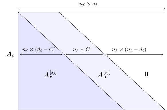
Figure 12: Part of the observation matrix related to a single location, $s_{j}$; observations for this location are then ordered in time with later observations towards the bottom. The matrix consists of three main parts: 1) Left triangle $\bm{A}_{c}^{[s_{j}]}$ — The mapping for well mixed fluxes; 2) Band: $\bm{A}_{a}^{[s_{j}]}$ — The mapping for the $C$ most recent flux fields; and 3) Right triangle: Zero-values indicating no sensitivity to future fluxes. A row in the matrix, as indicated by $\bm{A}_{i}$, gives the sensitivities for a single observation taken at time $d_{i}$.

The cost for solving the latter equation system can be greatly reduced by making use of the Kronecker structure of $\bm{R}_{\omega}$ and the structure of the observation matrix, $\bm{A}_{\omega}=\bm{J}\bm{L_{\omega}}$. For the remainder of this section we simplify the notation by dropping the $\bm{\omega}$-subscripts. In Section 2 we noted that the transport matrix could be divided into two sub-matrices, $\bm{J}=\begin{bmatrix}\bm{J}_{c}&\bm{J}_{a}\end{bmatrix}$, with sensitivities to well mixed fluxes, and recent fluxes, respectively. The structure of the observation matrix at a single site, $s_{j}$, is illustrated in Figure 12. Here, $\bm{A}_{c}^{[s_{j}]}$ and $\bm{A}_{a}^{[s_{j}]}$ represents the non-zero elements of rows in $\bm{J}_{c}\bm{L_{\omega}}$ and $\bm{J}_{a}\bm{L_{\omega}}$, corresponding to location $s_{j}$.

First, we note that,

$$\bm{R}^{T}\bm{S}^{T}=\bm{A}^{T}\Longleftrightarrow\bm{R}^{T}\bm{S}_{i}^{T}=\bm{A}_{i}^{T},\quad i=1,\ldots n_{\text{obs}}$$ (67)

where $\bm{A}_{i}$ is the $i^{\text{th}}$ row in $\bm{A}$. Using the Kronecker structure of $\bm{R}=\bm{R}_{T}\otimes\bm{R}_{S}$ we have (Fernandes et al.,, 1998),

$$\bm{R}^{T}\bm{S}_{i}^{T}=\bm{A}_{i}^{T} \Leftrightarrow\bm{S}_{i}^{T}={(\bm{R}_{T}^{T}\otimes\bm{R}_{S}^{T})}^{-1}\bm{A}_{i}^{T}$$

$$\Leftrightarrow\bm{S}_{i}^{T}=(\bm{R}_{T}^{-T}\otimes\bm{R}_{S}^{-T})\bm{A}_{i}^{T}$$

$$\Leftrightarrow\bm{S}_{i}^{T}=\text{vec}\left(\bm{R}_{S}^{-T}\text{ivec}(\bm{A}_{i}^{T})\bm{R}_{T}^{-1}\right)$$

$$\Leftrightarrow\bm{S}_{i}^{T}=\text{vec}\left(\left(\bm{R}_{T}^{-T}(\bm{R}_{S}^{-T}\text{ivec}(\bm{A}_{i}^{T}))^{T}\right)^{T}\right),$$

where $\text{ivec}(\bm{A}_{i}^{T})$ is the column vector $\bm{A}_{i}^{T}$ of length $n_{\ell}n_{t}$, reshaped to a matrix of size, $n_{\ell}\times n_{t}$, as illustrated in Figure 13. The first $d_{i}-C$ columns in $\bm{A}_{i}$ are equal (sensitivities to well mixed fluxes), the next $C$ columns represent sensitivities to the $C$ flux fields just before observational time, and the following $n_{t}-d_{i}$ columns are zero (sensitivities to future fluxes). Moreover, the columns representing sensitivities to well mixed fluxes are the same for all observations. As a result, $\bm{R}_{S}^{-T}\text{ivec}(\bm{A}_{i}^{T})$ is achieved by essentially computing only the ”recent” part $\bm{R}_{S}^{-T}\text{ivec}(\bm{A}_{{a,i}}^{T})$ at a cost of $\mathcal{O}(Cn_{\ell}\log n_{\ell})$. With a total cost of $\mathcal{O}(n_{\text{obs}}Cn_{\ell}\log n_{\ell}+n_{\ell}\log n_{\ell})$ across all observations, since $\bm{R}_{S}$ will have $\mathcal{O}(n_{\ell}\log n_{\ell})$ non-zero elements (Rue and Held,, 2004, p. 51) and we can reuse the $\bm{R}_{S}^{-T}\text{ivec}(\bm{A}_{{c,i}}^{T})$ computations for the constant part.

For the temporal component the sparse triangular systems has to be solved for all observations and locations resulting in a total cost of $\mathcal{O}(n_{\text{obs}}n_{t}n_{\ell})=\mathcal{O}(n_{\text{obs}}n_{\omega})$, which is the dominating factor when computing $\bm{S}=\bm{A}\bm{R}_{z}^{-1}$.

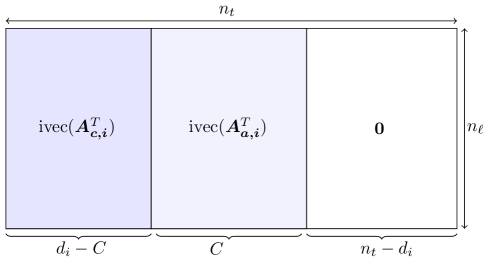
Figure 13: The matrix $ivec(\bm{A}_{i}^{T})$, composed into sub-matrices $ivec(\bm{A}_{{c,i}}^{T})$, $ivec(\bm{A}_{{a,i}}^{T})$, and a zero matrix.

S2.4 Computational costs

Considering the necessary computations; the Choleskey factors $\bm{R}_{t}$, $\bm{R}_{s}$, and $\bm{L}$ scale as $\mathcal{O}(n_{t})$, $\mathcal{O}(n_{s}^{3/2})$ and $\mathcal{O}(n_{\text{obs}}^{3})$, respectively. The different computational cost depends on the sparsity due to the temporal and spatial GMRFs (Rue and Held,, 2004, Ch. 2.4). Given the Choleskey factors, computation of the determinants is linear, since the determinant of a triangular matrix is computed as the product of the diagonal elemets: $\lvert\bm{L}\rvert=\prod_{i}\bm{L}_{ii}$. As described above the cost of computing $\bm{S}=\bm{A}\bm{R}_{z}^{-1}$, using back substitution and vectorization of the Kronecker product, is $\mathcal{O}(n_{\omega}n_{\text{obs}})$.

This makes the $\bm{S}\bm{S}^{T}$-product in (62) the most expensive calculation in (63) and (65), at a cost of $\mathcal{O}(n_{\text{obs}}^{2}n)$ since we typically have $n>n_{\text{obs}}$.

Appendix S3 Additional figures and results

Table 9: Observation class (last column) and reconstruction errors for all observations sites. The mean mismatch (bias) and RMSE were computed by comparing observed time-series of $\text{CO}_{2}$ from 01/1996 to 12/2000 with those obtained from the reconstructed fields using either the prior mean fluxes (a-prior) or conditional expectations from the spatio-temporal model (a-posteriori). Apart from the six validation locations marked in grey, the sites were used when computing the conditional expectations (i.e. they represent in-sample validation).

Location	Mean bias (ppm)		RMSE (ppm)		Class
	a-priori	a-posteriori	a-priori	a-posteriori
alt	2.385	-0.193	3.673	0.927	S
asc	1.113	0.050	1.514	0.356	R
ask	2.298	0.012	2.965	0.237	R
azr	2.057	0.048	2.764	0.946	R
bal	1.240	-0.120	4.087	2.123	C
bme	2.006	0.145	2.661	0.687	R
bmw	1.772	0.042	2.533	0.701	R
brw	2.111	0.089	3.661	0.361	S
bsc	-3.471	-0.279	6.985	2.254	C
cba	1.181	-0.579	3.547	1.234	S
cfa	0.568	0.001	1.436	0.730	S
cgo	0.579	-0.042	0.704	0.158	S
chr	1.046	0.624	1.412	0.980	R
cmn	3.531	0.875	5.451	2.409	C
cmo	1.829	0.147	3.966	1.275	S
crz	0.248	-0.013	0.667	0.444	R
eic	1.620	0.234	1.788	0.628	R
epc	2.128	0.062	4.091	1.547	S
gmi	1.436	0.077	2.115	0.700	R
goz	2.393	0.164	3.058	1.225	R
hba	0.369	0.071	0.580	0.231	R
hun	0.035	0.049	7.409	2.534	C
hun115	0.771	-0.661	6.216	1.741	C
ice	2.248	-0.009	3.621	0.597	R
itn	0.439	-0.793	3.663	2.179	C
izo	1.897	-0.109	2.652	0.549	R
key	1.138	-0.652	2.551	2.214	S
kum	1.549	-0.242	2.216	0.843	R
lef	2.365	-0.382	5.017	2.793	C
maa	0.298	0.075	0.489	0.197	R
mbc	2.031	-0.007	3.049	0.234	S
mhd	1.739	-0.697	3.709	1.887	S
mid	1.595	0.074	2.310	0.593	R
mlo	1.811	0.195	2.211	0.472	R
mqa	0.348	0.005	0.527	0.219	R
nwr	2.399	0.043	3.116	0.789	M
pal	2.301	-0.077	4.433	0.945	C
poc000	0.592	-0.272	2.329	1.556	R
pocn05	0.980	0.165	1.767	0.825	R
pocn1	0.634	-0.514	2.908	2.534	R
pocn15	1.535	0.182	2.693	1.105	R
pocn20	0.948	-0.358	3.501	2.253	R
pocn25	1.344	-0.070	2.934	1.171	R
pocn30	1.808	-0.057	3.105	1.106	R
pocs05	1.175	0.035	1.571	0.580	R
pocs10	0.838	-0.037	1.745	1.036	R
pocs15	1.026	0.050	1.366	0.589	R
pocs20	0.692	0.105	1.394	0.531	R
pocs25	0.406	0.002	1.499	0.852	R
pocs30	0.664	0.076	1.093	0.610	R
pocs35	0.210	-0.133	0.914	0.693	R
prs	3.055	0.737	4.088	1.470	C
psa	-0.273	-0.169	0.544	0.432	R
rpb	1.875	0.068	2.664	0.503	R
sch	4.905	0.054	5.879	0.501	R
sey	1.052	-0.134	1.351	0.601	R
shm	3.167	0.087	5.111	0.550	R
sis	2.525	-0.052	3.762	0.741	R
smo	1.319	0.012	1.455	0.313	R
spo	0.279	-0.052	0.498	0.135	R
stm	1.772	0.032	3.078	0.469	S
syo	-0.041	-0.261	0.595	0.483	R
tap	0.722	-0.164	3.816	2.197	S
tdf	0.089	0.075	0.740	0.429	S
uta	2.732	0.090	3.431	1.074	C
uum	2.335	-0.008	3.797	1.147	C
wes	0.857	-0.077	4.121	1.138	S
wis	1.731	-0.013	3.154	0.968	C
wlg	2.976	0.004	3.907	0.313	M
zep	2.099	-0.026	3.377	0.611	R

S3.1 Flux anomalies for January, April, and October 1999

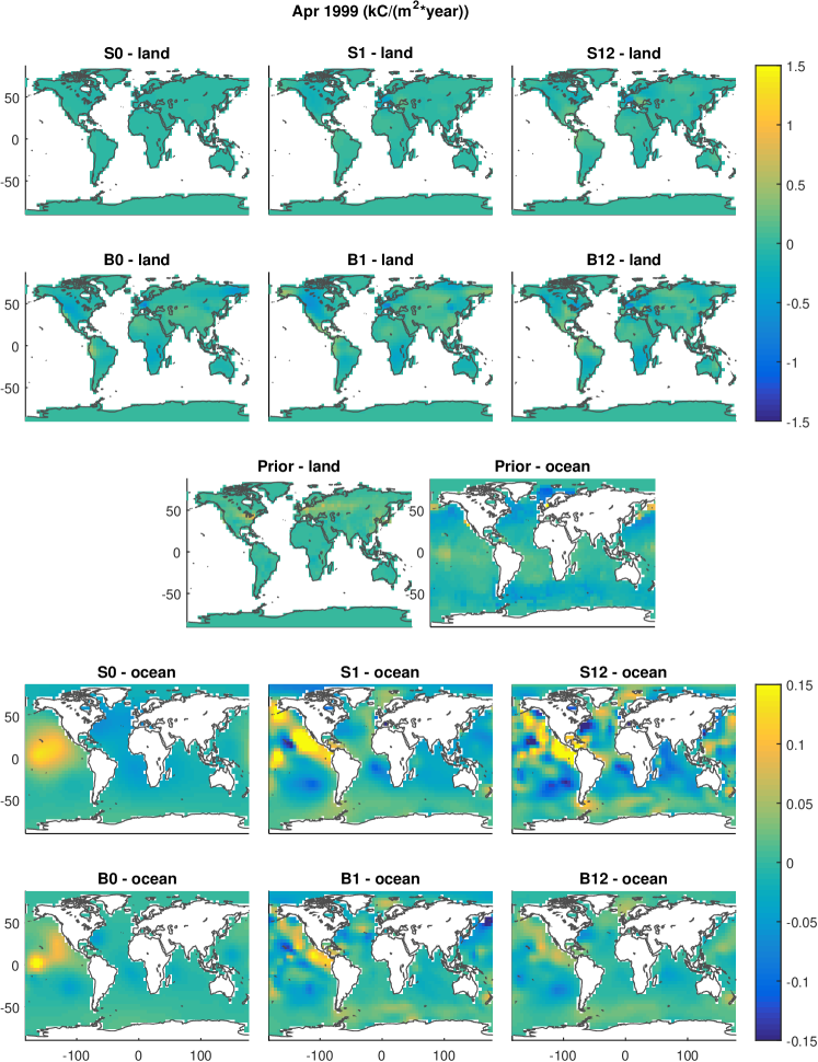
Figure 16: Flux anomalies for April 1999, using the six different models. The first two rows show the estimated land flux anomalies, the third row shows the prior mean land and ocean fluxes, and the last two rows display the estimated ocean anomalies. Note that the colour scale differs for land and ocean fluxes.

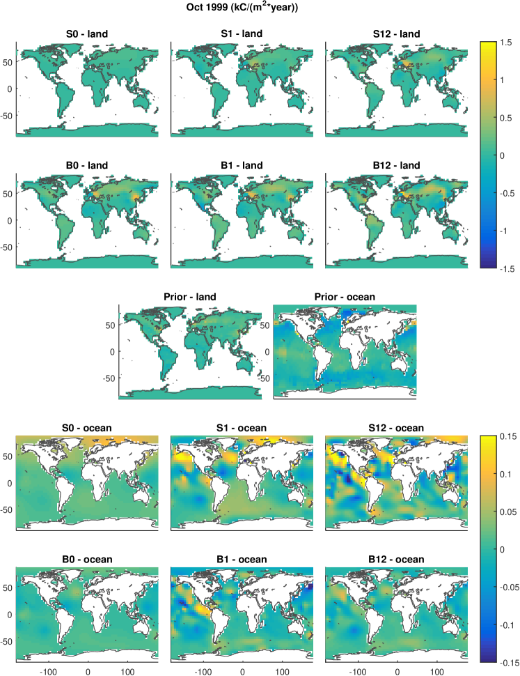
Figure 17: Flux anomalies for October 1999, using the six different models. The first two rows show the estimated land flux anomalies, the third row shows the prior mean land and ocean fluxes, and the last two rows display the estimated ocean anomalies. Note that the colour scale differs for land and ocean fluxes.

References

- Akaike, (1969) Akaike, H. (1969). Fitting autoregressive models for prediction. Annals of the Institute of Statistical Mathematics, 21:243–247.
- Andres et al., (1996) Andres, R. J., Marland, G., Fung, I., and Matthews, E. (1996). A 11∘ distribution of carbon dioxide emissions from fossil fuel consumption and cement manufacture, 1950-1990. Global Biogeochemical Cycles, 10(3):419–429.
- Baker et al., (2006) Baker, D., Law, R. M., Gurney, K. R., Rayner, P., Peylin, P., Denning, A., Bousquet, P., Bruhwiler, L., Chen, Y.-H., Ciais, P., et al. (2006). Transcom 3 inversion intercomparison: Impact of transport model errors on the interannual variability of regional CO2 fluxes, 1988–2003. Global Biogeochemical Cycles, 20(1).
- Bakka et al., (2018) Bakka, H., Rue, H., Fuglstad, G.-A., Riebler, A., Bolin, D., Illian, J., Krainski, E., Simpson, D., and Lindgren, F. (2018). Spatial modeling with R-INLA: A review. ”WIREs Comput. Stat.”, 10(6):e1443.
- Banerjee et al., (2008) Banerjee, S., Gelfand, A. E., Finley, A. O., and Sang, H. (2008). Gaussian predictive process models for large spatial data sets. Journal of the Royal Statistical Society: Series B, 70(4):825–848.
- Bekas et al., (2007) Bekas, C., Kokiopoulou, E., and Saad, Y. (2007). An estimator for the diagonal of a matrix. Applied numerical mathematics, 57(11-12):1214–1229.
- Blangiardo and Cameletti, (2015) Blangiardo, M. and Cameletti, M. (2015). Spatial and spatio-temporal Bayesian models with R-INLA. John Wiley & Sons.
- Boden et al., (2011) Boden, T. A., Marland, G., and Andres, R. J. (2011). Global, regional, and national fossil-fuel CO2 emissions, 1751–2008 (version 2011). Technical report, Carbon Dioxide Information Analysis Center CDIAC, Oak Ridge National Laboratory, Oak Ridge, TN.
- Bolin et al., (2011) Bolin, D., Lindgren, F., et al. (2011). Spatial models generated by nested stochastic partial differential equations, with an application to global ozone mapping. The Annals of Applied Statistics, 5(1):523–550.
- Bousquet et al., (2000) Bousquet, P., Peylin, P., Ciais, P., Le Quéré, C., Friedlingstein, P., and Tans, P. P. (2000). Regional changes in carbon dioxide fluxes of land and oceans since 1980. Science, 290(5495):1342–1346.
- Brenkert, (2003) Brenkert, A. L. (2003). Carbon dioxide emission estimates from fossil-fuel burning, hydraulic cement production, and gas flaring for 1995 on a one degree grid cell basis. [Available at http://cdiac.esd.ornl.gov/ndps/ndp058a.html].
- Brockwell, (2009) Brockwell, Peter J. adn Davis, R. A. (2009). Time Series: Theory and Methods. Springer, second edition.
- Enting, (2002) Enting, I. G. (2002). Inverse problems in atmospheric constituent transport. Cambridge University Press.
- Fernandes et al., (1998) Fernandes, P., Plateau, B., and Stewart, W. J. (1998). Efficient descriptor-vector multiplications in stochastic automata networks. Journal of the ACM, 45(3):381–414.
- Gelfand, (2010) Gelfand, A. E. (2010). Misaligned spatial data: The change of support problem. In Gelfand, A. E., Diggle, P., Guttorp, P., and Fuentes, M., editors, Handbook of Spatial Statistics, pages 517–539. Chapman & Hall/CRC.
- Gurney et al., (2003) Gurney, K. R., Law, R. M., Denning, A. S., Rayner, P. J., Baker, D., Bousquet, P., Bruhwiler, L., Chen, Y.-H., Ciais, P., Fan, S., et al. (2003). Transcom 3 CO2 inversion intercomparison: 1. annual mean control results and sensitivity to transport and prior flux information. Tellus B: Chemical and Physical Meteorology, 55(2):555–579.
- Gurney et al., (2004) Gurney, K. R., Law, R. M., Denning, A. S., Rayner, P. J., Pak, B. C., Baker, D., Bousquet, P., Bruhwiler, L., Chen, Y.-H., Ciais, P., et al. (2004). Transcom 3 inversion intercomparison: Model mean results for the estimation of seasonal carbon sources and sinks. Global Biogeochemical Cycles, 18(1).
- Guttorp and Gneiting, (2006) Guttorp, P. and Gneiting, T. (2006). Studies in the history of probability and statistics xlix on the matern correlation family. Biometrika, 93(4):989–995.
- Harville, (1997) Harville, D. A. (1997). Matrix Algebra From a Statistician’s Perspective. Springer, first edition.
- Heimann and Körner, (2003) Heimann, M. and Körner, S. (2003). The global atmospheric tracer model TM3: Model description and user’s manual release 3.8a. Technical Report 5, Max-Planck-Institut für Biogeochemie, Jena, Germany.
- Higdon, (2002) Higdon, D. (2002). Space and space-time modeling using process convolutions. In Quantitative methods for current environmental issues, pages 37–56. Springer.
- Houweling et al., (1999) Houweling, S., Kaminski, T., Dentener, F., Lelieveld, J., and Heimann, M. (1999). Inverse modeling of methane sources and sinks using the adjoint of a global transport model. Journal of Geophysical Research: Atmospheres, 104(D21):26137–26160.
- ICOS, (2019) ICOS (2019). ICOS carbon portal. https://www.icos-cp.eu/. accessed 2019-05-15.
- Ingebrigtsen et al., (2014) Ingebrigtsen, R., Lindgren, F., and Steinsland, I. (2014). Spatial models with explanatory variables in the dependence structure. Spatial Statistics, 8:20–38.
- Kaminski et al., (1999) Kaminski, T., Heimann, M., and Giering, R. (1999). A coarse grid three-dimensional global inverse model of the atmospheric transport: 2. inversion of the transport of CO2 in the 1980s. Journal of Geophysical Research: Atmospheres, 104(D15):18555–18581.
- Knorr, (2000) Knorr, W. (2000). Annual and interannual co2 exchanges of the terrestrial biosphere: Process-based simulations and uncertainties. Global Ecology and Biogeography, 9(3):225–252.
- Lang et al., (2015) Lang, A., Schwab, C., et al. (2015). Isotropic gaussian random fields on the sphere: regularity, fast simulation and stochastic partial differential equations. The Annals of Applied Probability, 25(6):3047–3094.
- Law et al., (2003) Law, R. M., Chen, Y.-H., Gurney, K. R., and Modellers, T.-. (2003). Transcom 3 CO2 inversion intercomparison: 2. sensitivity of annual mean results to data choices. Tellus B: Chemical and Physical Meteorology, 55(2):580–595.
- Le Quéré et al., (2018) Le Quéré, C., Andrew, R. M., Friedlingstein, P., Sitch, S., Hauck, J., Pongratz, J., Pickers, P. A., Korsbakken, J. I., Peters, G. P., Canadell, J. G., Arneth, A., Arora, V. K., Barbero, L., Bastos, A., Bopp, L., Chevallier, F., Chini, L. P., Ciais, P., Doney, S. C., Gkritzalis, T., Goll, D. S., Harris, I., Haverd, V., Hoffman, F. M., Hoppema, M., Houghton, R. A., Hurtt, G., Ilyina, T., Jain, A. K., Johannessen, T., Jones, C. D., Kato, E., Keeling, R. F., Goldewijk, K. K., Landschützer, P., Lefèvre, N., Lienert, S., Liu, Z., Lombardozzi, D., Metzl, N., Munro, D. R., Nabel, J. E. M. S., Nakaoka, S.-I., Neill, C., Olsen, A., Ono, T., Patra, P., Peregon, A., Peters, W., Peylin, P., Pfeil, B., Pierrot, D., Poulter, B., Rehder, G., Resplandy, L., Robertson, E., Rocher, M., Rödenbeck, C., Schuster, U., Schwinger, J., Séférian, R., Skjelvan, I., Steinhoff, T., Sutton, A., Tans, P. P., Tian, H., Tilbrook, B., Tubiello, F. N., van der Laan-Luijkx, I. T., van der Werf, G. R., Viovy, N., Walker, A. P., Wiltshire, A. J., Wright, R., Zaehle, S., and Zheng, B. (2018). Global carbon budget 2018. Earth System Science Data, 10(4):2141–2194.
- Lindgren and Rue, (2007) Lindgren, F. and Rue, H. (2007). Explicit construction of GMRF approximations to generalised Matérn fields on irregular grids. Technical Report 12, Centre for Mathematical Sciences, Lund University, Lund, Sweden.
- Lindgren et al., (2011) Lindgren, F., Rue, H., and Lindström, J. (2011). An explicit link between gaussian fields and gaussian markov random fields: the stochastic partial differential equation approach. Journal of the Royal Statistical Society: Series B, 73(4):423–498.
- Michalak et al., (2004) Michalak, A. M., Bruhwiler, L., and Tans, P. P. (2004). A geostatistical approach to surface flux estimation of atmospheric trace gases. Journal of Geophysical Research: Atmospheres, 109(D14).
- (33) Moraga, P., Cramb, S. M., Mengersen, K. L., and Pagano, M. (2017a). A geostatistical model for combined analysis of point-level and area-level data using INLA and SPDE. Spatial Statistics, 21:27–41.
- (34) Moraga, P., Cramb, S. M., Mengersen, K. L., and Pagano, M. (2017b). A geostatistical model for combined analysis of point-level and area-level data using INLA and SPDE. Spatial Statistics, 21:27–41.
- Mueller et al., (2008) Mueller, K. L., Gourdji, S. M., and Michalak, A. M. (2008). Global monthly averaged CO2 fluxes recovered using a geostatistical inverse modeling approach: 1. results using atmospheric measurements. Journal of Geophysical Research: Atmospheres, 113(D21).
- OCO-2, (2019) OCO-2 (2019). Orbiting carbon observatory-2 (OCO-2). https://ocov2.jpl.nasa.gov/. accessed 2019-05-15.
- Peters et al., (2005) Peters, W., Miller, J., Whitaker, J., Denning, A., Hirsch, A., Krol, M., Zupanski, D., Bruhwiler, L., and Tans, P. (2005). An ensemble data assimilation system to estimate CO2 surface fluxes from atmospheric trace gas observations. Journal of Geophysical Research: Atmospheres, 110(D24).
- Rayner et al., (1999) Rayner, P., Enting, I., Francey, R., and Langenfelds, R. (1999). Reconstructing the recent carbon cycle from atmospheric CO2, C and O2/N2 observations. Tellus B: Chemical and Physical Meteorology, 51(2):213–232.
- Rödenbeck, (2005) Rödenbeck, C. (2005). Estimating CO2 sources and sinks from atmospheric mixing ratio measurements using a global inversion of atmospheric transport. Technical Report 06, Max-Planck-Institut für Biogeochemie, Jena, Germany.
- Rödenbeck et al., (2003) Rödenbeck, C., Houweling, S., Gloor, M., and Heimann, M. (2003). CO2 flux history 1982–2001 inferred from atmospheric data using a global inversion of atmospheric transport. Atmospheric Chemistry and Physics, 3(6):1919–1964.
- Rue and Held, (2004) Rue, H. and Held, L. (2004). Gaussian Markov random fields: theory and applications. CRC Press.
- Rue et al., (2009) Rue, H., Martino, S., and Chopin, N. (2009). Approximate bayesian inference for latent gaussian models by using integrated nested laplace approximations. Journal of the Royal Statistical Society: Series B, 71(2):319–392.
- Schwarz et al., (1978) Schwarz, G. et al. (1978). Estimating the dimension of a model. The annals of statistics, 6(2):461–464.
- Simpson et al., (2016) Simpson, D., Illian, J., Lindgren, F., Sorbye, S., and Rue, H. (2016). Going off grid: Computationally efficient inference for log-gaussian cox processes. Biometrika, online:1–22.
- Takahashi et al., (2002) Takahashi, T., Sutherland, S. C., Sweeney, C., Poisson, A., Metzl, N., Tilbrook, B., Bates, N., Wanninkhof, R., Feely, R. A., Sabine, C., et al. (2002). Global sea–air CO2 flux based on climatological surface ocean pCO2, and seasonal biological and temperature effects. Deep Sea Research Part II: Topical Studies in Oceanography, 49(9-10):1601–1622.
- Whittle, (1954) Whittle, P. (1954). On stationary processes in the plane. Biometrika, pages 434–449.
- Woodbury, (1950) Woodbury, M. A. (1950). Inverting modified matrices. Memorandum Rept. 42, Statistical Research Group, Princeton University.
- Zupanski et al., (2007) Zupanski, D., Denning, A. S., Uliasz, M., Zupanski, M., Schuh, A. E., Rayner, P. J., Peters, W., and Corbin, K. D. (2007). Carbon flux bias estimation employing maximum likelihood ensemble filter (mlef). Journal of Geophysical Research: Atmospheres, 112(D17).