Warm-Started Optimized Trajectory Planning for ASVs

Abstract

We consider warm-started optimized trajectory planning for autonomous surface vehicles (ASVs) by combining the advantages of two types of planners: an A^⋆ implementation that quickly finds the shortest piecewise linear path, and an optimal control-based trajectory planner. A nonlinear 3-degree-of-freedom underactuated model of an ASV is considered, along with an objective functional that promotes energy-efficient and readily observable maneuvers. The A^⋆ algorithm is guaranteed to find the shortest piecewise linear path to the goal position based on a uniformly decomposed map. Dynamic information is constructed and added to the A^⋆-generated path, and provides an initial guess for warm starting the optimal control-based planner. The run time for the optimal control planner is greatly reduced by this initial guess and outputs a dynamically feasible and locally optimal trajectory.

1 Introduction

Motivated by potential for reduced costs, as well as safer and more environmentally friendly operations, technology for autonomous surface vehicles (ASVs) is being developed at a rapid pace. Several commercial actors are spearheading the search for solutions for safe, collision-free and reliable autonomous operations. Rolls-Royce and Finferries demonstrated the world’s first autonomous car ferry “Falco” in 2018 (Jallal, 2018), which navigated autonomously between two ports in Finland by combining advanced sensor technology and collision avoidance algorithms.

A prerequisite for safe and efficient operation is a well-functioning path or trajectory planning method. Such a method is responsible for providing the ASV with a safe trajectory that avoids static obstacles such as land and shallow waters. Depending on the type of operation, one might want to optimize the trajectory for various objectives, such as energy efficiency, speed or trajectory length.

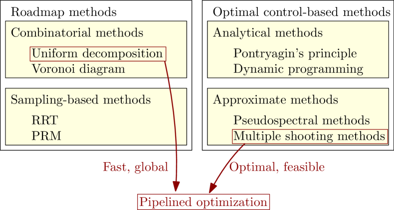
Figure 1: Categorization of some planning algorithms.

Numerous path and trajectory planning algorithms have been researched and are available for marine applications. One may categorize these planning algorithms as being roadmap-based or optimization-based. Figure 1 gives an overview of the categorization of some planning algorithm types. Roadmap methods are based on exploring points in the geometric space in order to build a path between the start and goal positions. There are two subcategories in roadmap methods. Combinatorial methods decompose an obstacle map using a preferred strategy, and perform a search in the resulting graph. The decomposition strategies include e.g. uniform grids, Voronoi diagrams and visibility graphs. The combinatorial methods explore the entire geometric space. The graph search is often performed using A^⋆, which is an efficient and well-known search algorithm widely used to solve path planning problems (Hart et al., 1968). A^⋆ guarantees to find the shortest path when using an admissible heuristic function. Hybrid A^⋆ extends the A^⋆ algorithm by generating dynamic trajectories to connect nodes, thus adding dynamic information to the search (Dolgov et al., 2010). As opposed to combinatorial methods, sampling-based methods randomly explores points in the map to build a path towards the goal. Probabilistic roadmap (PRM) is a sampling-based planning method that draws samples from the configuration space and connects them using a local planner (Kavraki et al., 1996). A graph search algorithm is applied to find the minimum cost path from start to goal in the resulting graph. Rapidly-exploring random tree (RRT) is another sampling-based method which calculates input trajectories between randomly sampled points and connects them in a tree until the start and goal positions are connected (LaValle, 1998). Although RRT uses a cost function, the method is not optimal and will lock into the first connection between start and goal. Various flavors of RRT are developed to amend this, e.g. RRT ^⋆ (Karaman and Frazzoli, 2011). This method continuously performs tree rewiring and has probabilistic completeness, but converges slowly.

The other group of planning methods contains algorithms based on optimal control. This group may further be divided into analytical and approximate methods. Analytical methods such as Pontryagin’s principle are only able to find solutions in very simple cases and are generally unpractical. Approximate methods such as e.g. pseudospectral optimal control (Bitar et al., 2018; Ross and Karpenko, 2012) are highly sensitive to initial guesses of the solution and will converge to a local optimum close to this guess. Without a good initial guess, they also experience long run times and are sensitive to problem dimensionality.

Zhang et al. (2018) plan trajectories for parking autonomous cars by combining hybrid A^⋆ with an optimal control-based method. Motivated by the same goals of exploiting the strengths and mitigate the weaknesses of optimal control-based algorithms, we here attempt to solve the long-term trajectory planning problem for ASVs as a transcribed optimal control problem (OCP), and warm start the solver using the smoothed solution of an A^⋆ geometric planner. In this three-step pipelined approach, the A^⋆ planner swiftly provides a set of waypoints representing the shortest path as Section 3. This path is converted into a full state trajectory by adding artificial and nearly feasible temporal information as Section 4. Section 5 takes this trajectory and uses it as the initial guess for an OCP solver, which finds an optimized trajectory near the globally shortest path. The structure of this pipelined concept is illustrated in Figure 2. The method is an off-line global planner, which assumes that information about the map and environment is known a priori.

Figure 2: Pipelined path planning concept.

The rest of this paper is organized as follows: Section 2 presents the mathematical model of the ASV used in simulations and planning. Finding the waypoints describing the shortest path with A^⋆ is described in Section 3, and Section 4 explains how the A^⋆ solution is converted to a trajectory. Section 5 shows how the OCP is transcribed to an nonlinear program (NLP), which yields an optimized trajectory when solved. Simulation scenarios and results are presented in Section 6, while Section 7 concludes the paper.

2 ASV modeling and obstacles

In (Loe, 2008), a simple nonlinear 3-degree-of-freedom ship model is identified to approximate the dynamics of the ASV Viknes 830. Without loss of generality for the method described in this paper, we use that model to perform trajectory planning. The model has the form

$$\dot{\bm{\eta}} =\bm{\mathrm{R}}(\psi)\bm{\nu}$$ (1a)

$$\bm{\mathrm{M}}\dot{\bm{\nu}}+\bm{\mathrm{C}}(\bm{\nu})\bm{\nu}+\bm{\mathrm{D}}(\bm{\nu})\bm{\nu} =\bm{\tau}(\bm{u})\,.$$ (1b)

The pose vector $\bm{\eta}=[x,y,\psi]^{\top}\in{}^{2}\times\operatorname{S}$ contains the ASV’s position and heading angle in the Earth-fixed North East Down (NED) frame. The velocity vector $\bm{\nu}=[u,v,r]^{\top}\in\mathbb{R}^{3}$ contains the ASV’s body-fixed velocities: surge, sway and yaw rate, respectively. The rotation matrix $\bm{\mathrm{R}}(\psi)$ transforms the body-fixed velocities to NED:

$$\bm{\mathrm{R}}(\psi)=\begin{bmatrix}\cos\psi&-\sin\psi&0\\ \sin\psi&\cos\psi&0\\ 0&0&1\end{bmatrix}.$$ (2)

The matrix $\bm{\mathrm{M}}\in{}^{3\times 3}$ represents system inertia, $\bm{\mathrm{C}}(\bm{\nu})\in{}^{3\times 3}$ Coriolis and centripetal effects, and $\bm{\mathrm{D}}(\bm{\nu})\in{}^{3\times 3}$ represents damping effects. The ASV is controlled by the control vector $\bm{u}=[X,N]^{\top}\in{}^{2}$, which contains surge force and yaw moment. The control vector is mapped to a force vector $\bm{\tau}(\bm{u})=[X,0,N]^{\top}$. The ASV’s states are collected in the vector $\bm{x}=[x,y,\psi,u,v,r]^{\top}$, and we collect the dynamic model (1) in the following compact form for notational ease in the remainder of the paper:

$$\dot{\bm{x}}=\bm{f}(\bm{x},\bm{u})=\begin{bmatrix}\bm{\mathrm{R}}(\psi)\bm{\nu}\\ \bm{\mathrm{M}}^{-1}\left(-\bm{\mathrm{C}}(\bm{\nu})\bm{\nu}-\bm{\mathrm{D}}(\bm{\nu})\bm{\nu}+\bm{\tau}(\bm{u})\right)\end{bmatrix}.$$ (3)

3 Step 1: A^⋆ path planner

To quickly find the global shortest collision-free path between a start and goal position, we use an A^⋆ implementation on a uniformly decomposed grid. The A^⋆ implementation is standard, and details may be found in e.g. (Hart et al., 1968). The search algorithm looks for collision-free paths between nodes in the uniform grid, and uses Euclidean distance as cost and heuristic functions.

The decomposition of the map affects the solution space and the run time for Section 3. Using a uniform grid with grid size $\Delta d>0$ too large will take paths going through narrow passages away from the solution space, and the desired shortest path may not be found. A smaller grid size will explore more options, but requires more evaluation, giving a longer run time. This uniform grid is in our case chosen for simplicity, however exploring other decompositions such as Voronoi diagrams or a non-uniform grid might be desirable for performance reasons.

4 Step 2: Trajectory generation

In order to use the shortest path generated by Section 3 as an initial guess for the OCP, we convert it to a trajectory based on straight segments and circle arcs using a nominal forward velocity $u_{\text{nom}}>0$. The trajectory generation consists of three sub-steps: waypoint reduction, waypoint connection, and adding dynamic information.

4.1 Waypoint reduction

Algorithm 1 is employed to reduce the A^⋆ path from Section 3 to a minimum number of waypoints. The algorithm outputs a reduced path as an ordered set of waypoints $\mathbb{P}=\mathinner{\left\{\bm{p}_{k}\in{}^{2}~{}|~{}k=1,\dots,N_{r}\right\}}$ where $N_{r}$ is the number of waypoints. The A^⋆ waypoints are denoted $\bm{p}^{\star}_{k}$ for $k=1,\dots,N_{\star}$, ordered from start to goal, where $N_{\star}$ is the number of waypoints.

Algorithm 1 Waypoint reduction algorithm.

1:procedure Reduce

2:     $i\leftarrow N_{\star}$; $\mathbb{P}\leftarrow\texttt{InitializePath}(\bm{p}^{\star}_{i})$

3:     do

4:         for $j=1$ to $i-1$ do

5:              if $\lnot\texttt{Collision}(\bm{p}^{\star}_{i},\bm{p}^{\star}_{j})$ then

6:                  $\texttt{AddPoint}(\mathbb{P},\bm{p}^{\star}_{j})$

7:                  $i\leftarrow j$

8:                  break                       

9:     while  $i>1$

4.2 Waypoint connection

The waypoints in the reduced path $\bm{p}_{k}\in\mathbb{P}$ are connected with straight segments and circle arcs to increase geometric feasibility. This is done by calculating the parameters of a circle based on a radius of acceptance $R_{\text{acc}}>0$. The result is a path with discontinuous turn rate since the turn rate of such a curve will experience jumps at the beginning and end of the circle arcs. However, if the circle arcs have a turning radius $R_{\text{turn}}>0$ larger than the minimum turning radius of the ASV $R_{\text{turn},\text{min}}>0$, the resulting geometry of the path can be followed tightly. Additional information about such a path waypoint connection is available in (Fossen, 2011).

For each straight segment, the turn rate is $0$. For the circle arcs, the turn rate is $\nicefrac{{u_{\text{nom}}}}{{R_{\text{turn},k}}}$, where $R_{\text{turn},k}>0$ is the turning radius for arc $k$. The tangent angles for the straight segments are $\gamma_{k}\in\operatorname{S}$, and for the circle arcs, the tangent angles move between $\gamma_{k}$ and $\gamma_{k+1}$, depending on how far along the curve it is evaluated.

Using this information, we can concatenate a path consisting of alternations of straights and circle arcs, and construct a path function parametrized by length with position

$$\bm{p}_{g}\mathrel{\mathop{\mathchar 58\relax}}[0,L_{\text{path}}]\to{}^{2}\,,$$ (4a)

where $$L_{\text{path}}>0$$ is the total length of the path. Functions for path tangential angle and turn rate are also constructed:

$$\gamma_{g} \mathrel{\mathop{\mathchar 58\relax}}[0,L_{\text{path}}]\to\operatorname{S}\text{, and}$$ (4b)

$$r_{g} \mathrel{\mathop{\mathchar 58\relax}}[0,L_{\text{path}}]\to\real\,,$$ (4c)

respectively. These functions are subscripted by $(\cdot)_{g}$ to indicate that they are based on the path geometry.

4.3 Adding temporal information

After obtaining an arc-length parametrized path we add temporal information by assuming a constant surge velocity $u_{\text{nom}}$, a sway velocity $v$ of zero, and piecewise constant yaw rate $r$. The nominal surge velocity is determined by $u_{\text{nom}}=\frac{L_{\text{path}}}{t_{\text{max}}}$, where $t_{\text{max}}>0$ is the tunable time to complete the trajectory, which is valid on $t\in[0,t_{\text{max}}]$. The distance traveled will be $L(t)=u_{\text{nom}}\cdot t$, and the states will then have trajectories

$$\begin{bmatrix}x_{w}(t)&y_{w}(t)\end{bmatrix}^{\top} =\bm{p}_{g}(L(t))$$ (5a)

$$\psi_{w}(t) =\gamma_{g}(L(t))$$ (5b)

$$u_{w}(t) =u_{\text{nom}}$$ (5c)

$$v_{w}(t) =0$$ (5d)

$$r_{w}(t) =r_{g}(L(t))\,.$$ (5e)

The input trajectory is set to the constant values

$$\tau_{X,w}(t)=\tau_{X,ss},\quad\tau_{N,w}(t)=0\,$$ (6)

where $\tau_{X,ss}\in\real$ is calculated as the steady-state value required to maintain nominal forward velocity $u_{\text{nom}}$. The trajectories are subscripted by $(\cdot)_{w}$ to indicate that they will be used for warm-starting the OCP in Section 5.

The resulting trajectory is not dynamically feasible according to (1) but will be used as an initial guess for the OCP solver, described in the next section. The trajectory is collected in the following vectors:

$$\bm{x}_{w}(t)=\begin{bmatrix}x_{w}(t)\\ y_{w}(t)\\ \psi_{w}(t)\\ u_{w}(t)\\ v_{w}(t)\\ r_{w}(t)\end{bmatrix}\ \bm{u}_{w}(t)=\begin{bmatrix}\tau_{X,w}(t)\\ \tau_{N,w}(t)\end{bmatrix}\ \forall\,t\in[0,t_{\text{max}}]\,.$$ (7)

The goal of the method described in this paper is to find a trajectory of states and inputs that minimizes a cost functional $J(\bm{x}(\cdot),\bm{u}(\cdot))$:

$$J(\bm{x}(\cdot),\bm{u}(\cdot))=\int_{0}^{t_{\text{max}}}F(\bm{x}(\tau),\bm{u}(\tau))\operatorname{d\!}\tau\,,$$ (8)

which is dependent on a cost-to-go function $F(\bm{x},\bm{u})$. This function may be selected to find e.g. the trajectory that minimizes energy usage. The initial guess for the cost trajectory $J_{w}(\cdot)$ at time $t$ is determined by

$$J_{w}(t)=\int_{0}^{t}F(\bm{x}_{w}(\tau),\bm{u}_{w}(\tau))\operatorname{d\!}\tau\,.$$ (9)

5 Step 3: Optimal control

Optimal control is used to make feasible and optimize the trajectory provided by Section 4. An OCP is formulated as

$$\min_{\bm{x}(\cdot),\bm{u}(\cdot)}\int_{0}^{t_{\text{max}}}F(\bm{x}(\tau),\bm{u}(\tau))\operatorname{d\!}\tau$$ (10a)

subject to

$$\dot{\bm{x}}(t)=\bm{f}(\bm{x}(t),\bm{u}(t))~{}\forall t\in[0,t_{\text{max}}]$$ (10b)

$$\bm{h}(\bm{x}(t),\bm{u}(t))\leq\bm{0}~{}\forall t\in[0,t_{\text{max}}]$$ (10c)

$$\bm{e}(\bm{x}(0),\bm{x}(t_{\text{max}}))=\bm{0}\,.$$ (10d)

The solution of this OCP gives a trajectory of states $\bm{x}(\cdot)$ and inputs $\bm{u}(\cdot)$ that minimizes (8).

5.1 Cost functional

The cost functional described in (8) is dependent on the cost-to-go function $F(\bm{x},\bm{u})$. This function may be adjusted and structured according to the desired sense of optimality. Our aim is a trajectory which is optimized for energy usage, as well as performing readily observable maneuvers, as is required by International Regulations for Preventing Collisions at Sea (COLREGs) Rule 8. This results in a two-part cost-to-go function:

$$F(\bm{x},\bm{u})=K_{e}F_{e}(\bm{x},\bm{u})+K_{t}F_{t}(\bm{x})\,,$$ (11)

with tuning parameters $K_{e},K_{t}>0$. The first term penalizes energy usage and describes work done by the actuators:

$$F_{e}(\bm{x},\bm{u})=\mathinner{\!\left\lvert u\cdot\tau_{X}\right\rvert}+\mathinner{\!\left\lvert r\cdot\tau_{N}\right\rvert}\,.$$ (12)

The second term is a disproportionate penalization on turn-rate $r$, which prefers readily observable turns performed with high turn-rate. The function has the form

$$F_{t}(\bm{x})=\left(a_{t}r^{2}+(1-e^{-\frac{r^{2}}{b_{t}}})\right)\frac{1}{F_{t,max}}\,,$$ (13)

where

$$F_{t,max}=a_{t}r_{\text{max}}^{2}+(1-e^{-\frac{r_{\text{max}}^{2}}{b_{t}}})\,,$$ (14)

and $r_{\text{max}}>0$ is the ASV’s maximum yaw rate. The tuning parameters $a_{t}>0$ and $b_{t}>0$ shape the penalization to prefer higher or lower turn-rate, which is an idea obtained from (Eriksen and Breivik, 2017).

5.2 Obstacles

Obstacles are encoded as elliptic inequalities in (10c). The basis for one elliptic obstacle is

$$\left(\frac{x-x_{c}}{x_{a}}\right)^{2}+\left(\frac{y-y_{c}}{y_{a}}\right)^{2}\geq 1\,,$$ (15)

where $x_{c}$ and $y_{c}$ describe the ellipse center and $x_{a}$ and $y_{a}$ describe the sizes of the two elliptic axes. The ellipses are rotated by $\alpha$, which is the angle between the global $x$-axis and the direction of $x_{a}$. The resulting inequality becomes

$$g_{o}(x,y,x_{c},y_{c},x_{a},y_{a},\alpha)=\\ -\log\bigg{[}\left(\frac{(x-x_{c})\cos\alpha+(y-y_{c})\sin\alpha}{x_{a}}\right)^{2}\\ +\left(\frac{-(x-x_{c})\sin\alpha+(y-y_{c})\cos\alpha}{y_{a}}\right)^{2}+\epsilon\bigg{]}\\ +\log(1+\epsilon)\leq 0\,,$$ (16)

where a small value $\varepsilon>0$ is added to deal with feasibility issues as $x\to x_{c}$ and $y\to y_{c}$, and the logarithmic function is used to reduce numerical sizes, without changing the inequality. The same function is used in (Bitar et al., 2019).

5.3 NLP transcription

A multiple-shooting approach is used to transcribe the OCP into an NLP:

$$\min_{\bm{w}}\phi(\bm{w})$$ (17a)

subject to

$$\bm{g}_{lb}\leq\bm{g}(\bm{w})\leq\bm{g}_{ub}$$ (17b)

$$\bm{w}_{lb}\leq\bm{w}\leq\bm{w}_{ub}\,.$$ (17c)

The dynamics are discretized into $N_{ocp}$ steps in time, with step length $h=\nicefrac{{t_{\text{max}}}}{{N_{ocp}}}$. The decision variables $\bm{w}$ consist of the state variables $\bm{x}_{k}=\bm{x}(t_{k}),\,k=0,1,\dots,N_{ocp}$, the accumulated costs $J_{k}=J(t_{k}),\,k=0,1,\dots,N_{ocp}$, where

$$J(t)=\int_{0}^{t}F(\bm{x}(\tau),\bm{u}(\tau))\operatorname{d\!}\tau\,,$$ (18)

and the control inputs $\bm{u}_{k}=\bm{u}(t_{k}),\,k=0,1,\dots,N_{ocp}-1$:

$$\bm{w}=\begin{bmatrix}\bm{z}_{0}^{\top}&\bm{u}_{0}^{\top}&\bm{z}_{1}^{\top}&\dots&\bm{u}_{N_{ocp}-1}^{\top}&\bm{z}_{N_{ocp}}^{\top}\end{bmatrix}^{\top},$$ (19)

where $\bm{z}_{k}=[\bm{x}_{k}^{\top},J_{k}]^{\top}$.

The cost function (17a) approximates (10a) and is

$$\phi(\bm{w})=J_{N_{ocp}}\,.$$ (20)

The constraints (17b) are used to satisfy shooting constraints, as well as the collision avoidance constraints. For the shooting constraints, we construct a discrete representation of the dynamics (10b) as well as the integral (18) using a RK4 scheme with $K_{ocp}$ steps. We define the discrete version of (10b) augmented with the time derivative of (18) as

$$\bm{z}_{k+1}=\bm{F}(\bm{z}_{k},\bm{u}_{k})\,,$$ (21)

and construct the shooting constraints

$$\bm{g}_{s}(\bm{w})=\begin{bmatrix}\bm{z}_{1}-\bm{F}(\bm{z}_{0},\bm{u}_{0})\\ \vdots\\ \bm{z}_{N_{ocp}}-\bm{F}(\bm{z}_{N_{ocp}-1},\bm{u}_{N_{ocp}-1})\end{bmatrix},$$ (22)

with associated lower and upper bounds

$$\bm{g}_{s,lb}=\bm{g}_{s,ub}=\bm{0}_{(n+1)\cdot N_{ocp}}\,.$$ (23)

For obstacles $i=1,2,\dots,N_{o}$, we avoid collisions by satisfying the inequality constraint

$$g_{o}(x_{k},y_{k},x_{c,i},y_{c,i},a_{i},b_{i},\alpha_{i})\leq 0\,,$$ (24)

where $x_{k}=x(t_{k})$ and $y_{k}=y(t_{k})$ for $k=1,2,\dots,N_{ocp}$. We create a vector for all our obstacles in a single time step:

$$\begin{gathered}\bar{\bm{g}}_{o}(\bm{x}_{k})=\\ \begin{bmatrix}g_{o}(x_{k},y_{k},x_{c,1},y_{c,1},a_{1},b_{1},\alpha_{1})\\ g_{o}(x_{k},y_{k},x_{c,2},y_{c,2},a_{2},b_{2},\alpha_{2})\\ \vdots\\ g_{o}(x_{k},y_{k},x_{c,N_{o}},y_{c,N_{o}},a_{N_{o}},b_{N_{o}},\alpha_{N_{o}})\end{bmatrix}.\end{gathered}$$ (25)

Obstacle constraints for all time steps are gathered in

$$\bm{g}_{o}(\bm{w})=\begin{bmatrix}\bar{\bm{g}}_{o}(\bm{x}_{0})\\ \bar{\bm{g}}_{o}(\bm{x}_{1})\\ \vdots\\ \bar{\bm{g}}_{o}(\bm{x}_{N_{ocp}-1})\\ \end{bmatrix}$$ (26)

with associated lower and upper bounds

$$\bm{g}_{o,lb}=-\bm{\infty}_{N_{o}\cdot N_{ocp}}\quad\text{and}\quad\bm{g}_{o,ub}=\bm{0}_{N_{o}\cdot N_{ocp}}\,.$$ (27)

The nonlinear inequality constraints (17b) are completed as

$$\bm{g}_{lb}=\begin{bmatrix}\bm{g}_{s,lb}\\ \bm{g}_{o,lb}\end{bmatrix},~{}\bm{g}(\bm{w})=\begin{bmatrix}\bm{g}_{s}(\bm{w})\\ \bm{g}_{o}(\bm{w})\end{bmatrix},~{}\bm{g}_{ub}=\begin{bmatrix}\bm{g}_{s,ub}\\ \bm{g}_{o,ub}\end{bmatrix}.$$ (28)

The decision variable bounds (17c) are used to satisfy constant state and input constraints, as well as boundary conditions (10d). The bounds are

$$\begin{gathered}\bm{w}_{lb}^{\top}=\\ \begin{bmatrix}\bm{z}_{s,lb}^{\top}&\bm{u}_{lb}^{\top}&\bm{z}_{lb}^{\top}&\bm{u}_{lb}^{\top}&\dots&\bm{u}_{lb}^{\top}&\bm{z}_{f,lb}^{\top}\end{bmatrix}\end{gathered}$$ (29c)

$$\begin{gathered}\bm{w}_{ub}^{\top}=\\ \begin{bmatrix}\bm{z}_{s,ub}^{\top}&\bm{u}_{ub}^{\top}&\bm{z}_{ub}^{\top}&\bm{u}_{ub}^{\top}&\dots&\bm{u}_{ub}^{\top}&\bm{z}_{f,ub}^{\top}\end{bmatrix},\end{gathered}$$ (29f)

where

$$\bm{z}_{s,lb} =\begin{bmatrix}x_{s}&y_{s}&\psi_{lb}&u_{r,s}&0&0&0\end{bmatrix}^{\top}$$ (30a)

$$\bm{z}_{s,ub} =\begin{bmatrix}x_{s}&y_{s}&\psi_{ub}&u_{r,s}&0&0&0\end{bmatrix}^{\top}$$ (30b)

$$\bm{z}_{f,lb} =\begin{bmatrix}x_{f}&y_{f}&\psi_{lb}&u_{r,lb}&0&0&0\end{bmatrix}^{\top}$$ (30c)

$$\bm{z}_{f,ub} =\begin{bmatrix}x_{f}&y_{f}&\psi_{ub}&u_{r,ub}&0&0&\infty\end{bmatrix}^{\top}$$ (30d)

$$\bm{z}_{lb} =\begin{bmatrix}x_{lb}&y_{lb}&\psi_{lb}&u_{r,lb}&v_{lb}&r_{lb}&0\end{bmatrix}^{\top}$$ (30e)

$$\bm{z}_{ub} =\begin{bmatrix}x_{ub}&y_{ub}&\psi_{ub}&u_{r,ub}&v_{ub}&r_{ub}&\infty\end{bmatrix}^{\top}$$ (30f)

$$\bm{u}_{lb} =\begin{bmatrix}X_{lb}&N_{lb}\end{bmatrix}^{\top}$$ (30g)

$$\bm{u}_{ub} =\begin{bmatrix}X_{ub}&N_{ub}\end{bmatrix}^{\top},$$ (30h)

and where values subscripted with $(\cdot)_{s}$ represent initial conditions, $(\cdot)_{f}$ the final conditions, and $(\cdot)_{lb}$ and $(\cdot)_{ub}$ represent lower and upper bounds, respectively.

5.4 Initial guess and solver

The trajectories $\bm{x}_{w}(\cdot)$, $\bm{u}_{w}(\cdot)$ and $J_{w}(\cdot)$ from Section 5.4 are used as an initial guess to warm-start the NLP. These trajectories are sampled at the time steps $t_{k}$, $k=0,\dots,N_{ocp}$ using interpolation, and shaped into the form of the decision vector $\bm{w}$ (19), providing the initial guess $\bm{w}_{0}$.

The NLP as defined by (17) is solved by the interior-point method Ipopt (Wächter and Biegler, 2005) using Casadi (Andersson et al., 2018) for Matlab.

5.5 Algorithm summary

The pipelined algorithm is summarized by the steps in Table 1, where the properties of each step are highlighted in terms of parametrization, feasibility according to (1) and optimality.

Table 1: Algorithm step explanation.

Step	Parametrized by	Dynamic feasibility	Optimality
3	Length	None, piecewise linear	Shortest piecewise linear path
4	Time	Discontinuous yaw rate $r$	None
5	Time	Adheres to (1)	Energy and COLREGs Rule 8

While Section 3 gives the shortest piecewise linear path, it is parametrized by length, and will not be dynamically feasible for warm-starting the OCP in Section 5. Section 4 connects the waypoints with circle arcs and adds artificial dynamics, which moves us closer to a dynamically feasible trajectory. However, we lose the optimality of the shortest path with this modification, and the yaw rate is discontinuous, which is not possible according to (1). This trajectory is usable as an initial guess for Section 5, which converges to a trajectory that adheres to (1), and adds optimality according to (10a).

6 Simulation scenarios and results

The scenario selected for testing our planning method is Sjernarøy north of Stavanger, Norway, near $59.25\text{\,}\frac{\mathrm{\SIUnitSymbolDegree}}{}$N and $5.83\text{\,}\frac{\mathrm{\SIUnitSymbolDegree}}{}$E. A map of this scenario is shown in Figure 3. The scenario has many possible routes between the start and goal positions, including routes that go outside the islands, and the narrow passage between the islands. The narrow passage is the shortest path, and one could claim that in the absence of disturbances, this shortest path is also the most energy efficient. However, since the problem of finding this path is non-convex and resembles an integer problem, the OCP alone would struggle to find the shortest path. We use the algorithm parameters presented in Table 2.

Table 2: Parameter values.

Param.	Val.	Param.	Val.
$\Delta d$	$50\text{\,}\mathrm{[}\mathrm{m}\mathrm{]}$	$t_{\text{max}}$	$2200\text{\,}\mathrm{[}\mathrm{s}\mathrm{]}$
$N_{ocp}$	$1000\text{\,}\frac{}{}$	$K_{ocp}$	$1\text{\,}\frac{}{}$
$K_{e}$	$3.5\text{⋅}{10}^{-4}\text{\,}\mathrm{[}\mathrm{J}^{-1}\mathrm{]}$	$K_{t}$	$800\text{\,}\frac{}{}$
$a_{t}$	$112\text{\,}\mathrm{[}\mathrm{s}\mathrm{{}^{2}}\mathrm{/}\mathrm{rad}\mathrm{{}^{2}}\mathrm{]}$	$b_{t}$	$6.25\text{⋅}{10}^{-5}\text{\,}\mathrm{[}\mathrm{rad}\mathrm{{}^{2}}\mathrm{/}\mathrm{s}\mathrm{{}^{2}}\mathrm{]}$
$R_{acc}$	$10\text{\,}\mathrm{[}\mathrm{m}\mathrm{]}$	$R_{\text{turn},\text{min}}$	$24.5\text{\,}\mathrm{[}\mathrm{m}\mathrm{]}$
$r_{\text{max}}$	$40\text{\,}\mathrm{[}\mathrm{\SIUnitSymbolDegree}\mathrm{/}\mathrm{s}\mathrm{]}$

To benchmark our planning algorithm, we apply it to the scenario illustrated in Figure 3 in Matlab on a laptop with an Intel Core i7-7700HQ processor. For comparison, we also apply the OCP to the same scenario without an initial guess, i.e. cold starting Section 5. Solutions from these two methods will be dynamically feasible trajectories with different routings to reach the goal position. We use metrics of total cost and run times to compare the algorithms. These metrics will also be applied to the trajectory after Section 4. This trajectory is not dynamically feasible according to (1) but can tell us how the smoothed A^⋆ trajectory performs without optimization.

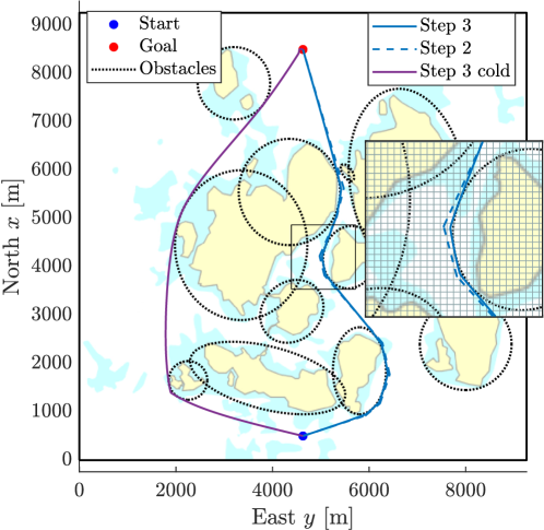
Figure 3: Map showing the scenario used for planning, with multiple elliptical obstacle boundaries surrounding the small islands. Trajectories after steps 4 and 5 are plotted. A cold-started solution is also included.

The resulting trajectories are plotted on top of the scenario in Figure 3. We see that the initial guess goes through the narrow passage between the islands and that the warm-started OCP finds a solution along the same route. As expected, the cold-started OCP goes outside the passage and finds a longer solution. A zoomed inset in Figure 3 shows how the OCP is able to produce readily observable maneuvers by making sharp turns around the obstacle boundaries. The inset also includes the grid used by Section 3.

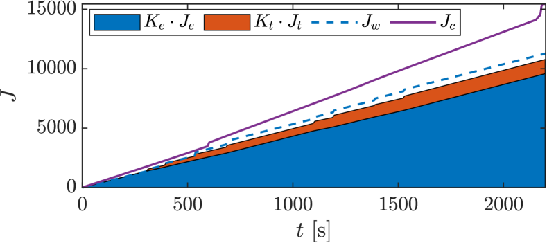
Figure 4: Cost functional development along both the optimized trajectory and the initial guess. The optimized trajectory shows the cost split into contributions from energy optimization and observable maneuvers. Also, the cost of the cold-started OCP is denoted $J_{c}$.

Figure 4 shows us the cost functional develops along the trajectories of the warm-started OCP ($K_{e}\cdot J_{e}+K_{t}\cdot J_{t}$), the initial guess ($J_{w}$) and the cold-started OCP ($J_{c}$). Table 3 shows the results at $t=t_{\text{max}}$ for the three methods. We see the scaled total cost as calculated by (10a) and (11), as well as the energy cost calculated by (12). An improvement of $30\text{\,}\frac{\mathrm{\char 37\relax}}{}$ is obtained by warm-starting the OCP compared to cold starting it, explained by the shorter route selection. The warm-started OCP is also able to improve on the dynamically infeasible initial guess by $4\text{\,}\frac{\mathrm{\char 37\relax}}{}$.

Table 3 also shows the run times of the three methods. Since the initial guess alone does not perform any iterative optimization, it has the lowest run time. The warm-started method spends $27\text{\,}\frac{\mathrm{s}}{}$ in total to find an optimized solution to the path planning problem, including $21\text{\,}\frac{\mathrm{s}}{}$ spent solving the OCP. This is an improvement of $84\text{\,}\frac{\mathrm{\char 37\relax}}{}$ compared to the cold-started OCP which spends approximately three minutes. The run-time cost of obtaining a feasible trajectory via optimal control is significant compared to performing A^⋆ and dynamic generation alone.

The state trajectories for the initial guess and warm-started OCP are shown in Figure 5. From the heading angle plot, we see that $\psi$ performs jumps of more than $30\text{\,}\frac{\mathrm{\SIUnitSymbolDegree}}{}$, which is a clear indication of intent to other vessels, even in situations with restricted visibility (Cockcroft and Lameijer, 2004). This is further observed in the yaw rate state $r$, where instead of having long turns with low yaw rate magnitude, we have abrupt turns with high-valued $r$. This is shown more clearly in Figure 6, which zooms in on a selected time interval.

Table 3: Scenario results.

	Warm started Section 5	Cold started Section 5	Section 4
Feasible	Yes	Yes	No
Scaled total cost ($J$)	$1.08\text{⋅}{10}^{4}\text{\,}\frac{}{}$	$1.54\text{⋅}{10}^{4}\text{\,}\frac{}{}$	$1.13\text{⋅}{10}^{4}\text{\,}\frac{}{}$
Unscaled energy cost ($J_{e}$)	$2.74\text{⋅}{10}^{7}\text{\,}\mathrm{[}\mathrm{J}\mathrm{]}$	$3.94\text{⋅}{10}^{7}\text{\,}\mathrm{[}\mathrm{J}\mathrm{]}$	$2.84\text{⋅}{10}^{7}\text{\,}\mathrm{[}\mathrm{J}\mathrm{]}$
Total run time	$26.7\text{\,}\mathrm{[}\mathrm{s}\mathrm{]}$	$174\text{\,}\mathrm{[}\mathrm{s}\mathrm{]}$	$5.7\text{\,}\mathrm{[}\mathrm{s}\mathrm{]}$
Section 3 run time	$3.4\text{\,}\mathrm{[}\mathrm{s}\mathrm{]}$	-	$3.4\text{\,}\mathrm{[}\mathrm{s}\mathrm{]}$
Section 4 run time	$2.2\text{\,}\mathrm{[}\mathrm{s}\mathrm{]}$	-	$2.2\text{\,}\mathrm{[}\mathrm{s}\mathrm{]}$
Section 5 run time	$21.1\text{\,}\mathrm{[}\mathrm{s}\mathrm{]}$	$174\text{\,}\mathrm{[}\mathrm{s}\mathrm{]}$	-
Section 5 iterations	58	549	-

Figure 5: State values for heading, velocities and yaw rate for both the optimized trajectory and the initial guess.

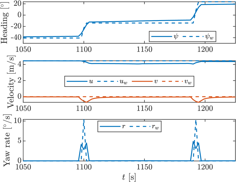
Figure 6: Zoomed-in section of Figure 5.

7 Conclusion

We have developed and demonstrated a pipelined trajectory planning algorithm that exploits the speed and global properties of an A^⋆ search with the optimality of an OCP solver. The results from Section 6 show that using the initial guess provided by a smoothed A^⋆ path in an OCP significantly improves both run time and optimality compared to a cold-started OCP alone. Performing optimization on the A^⋆ path significantly increases run time but will find a feasible locally optimal trajectory, as opposed to A^⋆ alone.

Qualitatively, the developed method is complete in terms of the shortest path, since this is the geometric objective of the A^⋆ implementation. This is dependent on the discretization of the map, since using larger grid spacing to reduce run time removes narrow passages from the solution space. Using a different discretization scheme such as e.g. Voronoi diagrams may guarantee a complete solution space. The developed method is also locally optimal in the sense of the provided objective, which is a combination of energy consumption and readily observable maneuvers in our case. The optimality is provided by the implemented OCP which alone is not able to find the global optimum, demonstrated by the cold-started result in Figure 3. However, the OCP warm-started by the shortest path found by the A^⋆ method is at least locally optimal and may be close to the global optimum, since, in the absence of disturbances, the shortest path is also the one that requires the least energy. In addition to improving optimality of the A^⋆ result, the OCP adds feasibility, unlike the A^⋆ consideration which is purely geometric. Using this warm-starting scheme is that the OCP will lock into one routing alternative. Depending on the desired sense of optimality, this may not be the desired solution, which is a disadvantage to some use cases.

The algorithm presented here has been used in a hybrid collision avoidance architecture in (Eriksen et al., 2019), where it is extended to include disturbances in the form of ocean currents.

Further work on this topic includes:

• Implementing a more general obstacle representation to handle a wider range of map representations. E.g. the obstacle representation in (Zhang et al., 2018) handles convex polygons as smooth inequality conditions.

• Improvements on the map discretization scheme are also desirable to reduce computational time of the A^⋆ algorithm while preserving completeness of the solution space.

• Additionally, an OCP representation that is parametrized by straight lines between waypoints in combination with full-state dynamics may be advantageous to inherently produce COLREGs-compliant trajectories.

References

- Andersson et al. (2018) Andersson, J. A. E., Gillis, J., Horn, G., Rawlings, J. B., and Diehl, M. (2018). CasADi – A software framework for nonlinear optimization and optimal control. Mathematical Programming Computation, 11(1):1–36.
- Bitar et al. (2018) Bitar, G., Breivik, M., and Lekkas, A. M. (2018). Energy-optimized path planning for autonomous ferries. In Proc. of the 11th IFAC CAMS, Opatija, Croatia, pages 389–394.
- Bitar et al. (2019) Bitar, G., Eriksen, B.-O.H., Lekkas, A. M., and Breivik, M. (2019). Energy-optimized hybrid collision avoidance for ASVs. In Proc. of the 17th ECC, Naples, Italy.
- Cockcroft and Lameijer (2004) Cockcroft, A. N. and Lameijer, J. N. F. (2004). A Guide to the Collision Avoidance Rules. Elsevier Butterworth-Heinemann.
- Dolgov et al. (2010) Dolgov, D., Thrun, S., Montemerlo, M., and Diebel, J. (2010). Path planning for autonomous vehicles in unknown semi-structured environments. The International Journal of Robotics Research, 29(5):485–501.
- Eriksen et al. (2019) Eriksen, B.-O.H., Bitar, G., Breivik, M., and Lekkas, A. M. (2019). Hybrid collision avoidance for ASVs compliant with COLREGs rules 8 and 13–17. arXiv:1907.00198 [eess.SY]. Submitted to Frontiers in Robotics and AI.
- Eriksen and Breivik (2017) Eriksen, B.-O.H. and Breivik, M. (2017). MPC-based mid-level collision avoidance for ASVs using nonlinear programming. In Proc. of the IEEE CCTA, Mauna Lani, HI, USA, pages 766–772.
- Fossen (2011) Fossen, T. I. (2011). Handbook of Marine Craft Hydrodynamics and Motion Control. Wiley-Blackwell.
- Hart et al. (1968) Hart, P., Nilsson, N., and Raphael, B. (1968). A formal basis for the heuristic determination of minimum cost paths. IEEE Transactions on Systems Science and Cybernetics, 4(2):100–107.
- Jallal (2018) Jallal, C. (2018). Rolls-Royce and Finferries demonstrate world’s first fully autonomous ferry. Maritime Digitalisation & Communications. Accessed 2019-04-11.
- Karaman and Frazzoli (2011) Karaman, S. and Frazzoli, E. (2011). Sampling-based algorithms for optimal motion planning. The International Journal of Robotics Research, 30(7):846–894.
- Kavraki et al. (1996) Kavraki, L. E., Svestka, P., Latombe, J.-C., and Overmars, M. H. (1996). Probabilistic roadmaps for path planning in high-dimensional configuration spaces. IEEE Transactions on Robotics and Automation, 12(4):566–580.
- LaValle (1998) LaValle, S. M. (1998). Rapidly-exploring random trees: A new tool for path planning. Technical report.
- Loe (2008) Loe, Ø. A. G. (2008). Collision avoidance for unmanned surface vehicles. Master’s thesis, Norwegian University of Science and Technology, Trondheim, Norway.
- Ross and Karpenko (2012) Ross, I. M. and Karpenko, M. (2012). A review of pseudospectral optimal control: From theory to flight. Annual Reviews in Control, 36(2):182–197.
- Wächter and Biegler (2005) Wächter, A. and Biegler, L. T. (2005). On the implementation of an interior-point filter line-search algorithm for large-scale nonlinear programming. Mathematical Programming, 106:25–57.
- Zhang et al. (2018) Zhang, X., Liniger, A., Sakai, A., and Borrelli, F. (2018). Autonomous parking using optimization-based collision avoidance. In Proc. of the IEEE CDC, Miami Beach, FL, USA, pages 4327–4332.