Interpretable Learning in Multivariate Big Data Analysis for Network Monitoring

Abstract

There is an increasing interest in the development of new data-driven models useful to assess the performance of communication networks. For many applications, like network monitoring and troubleshooting, a data model is of little use if it cannot be interpreted by a human operator. In this paper, we present an extension of the Multivariate Big Data Analysis (MBDA) methodology, a recently proposed interpretable data analysis tool. In this extension, we propose a solution to the automatic derivation of features, a cornerstone step for the application of MBDA when the amount of data is massive. The resulting network monitoring approach allows us to detect and diagnose disparate network anomalies, with a data-analysis workflow that combines the advantages of interpretable and interactive models with the power of parallel processing. We apply the extended MBDA to two case studies: UGR’16, a benchmark flow-based real-traffic dataset for anomaly detection, and Dartmouth’18, the longest and largest Wi-Fi trace known to date.

I Introduction

In the Big Data era, there is an increasing interest in the development of new data analysis methods to improve the performance of communication networks, in tasks like network monitoring, troubleshooting and optimization [1]. The current trend in data analysis is towards highly complex black-box methodologies, like deep learning [2]. These methodologies learn models of the data intended to be used automatically, and with little or no human supervision or interaction. Unfortunately, for many network applications, a model of the data is of little use if it cannot be interpreted by a human operator.

The relevance of interpretable models in several applications has raised a lot of attention in the research community in recent years [3]. There are two basic approaches to the derivation of interpretable models from data. On the one hand, the need for the interpretation of black-box models has given rise to concepts like interpretable or explainable machine learning [4], where strategies to explain black-box models or to calibrate more interpretable black-box models are pursued. An alternative approach is to use data analysis methods that are themselves interpretable, rather than black-box [5]. This paper lies in the second category.

Just like their black-box counterparts, interpretable models can be useful in classification, regression and anomaly detection tasks. However, a major advantage of interpretable models is that they also provide information about why a model gives a certain output. There are many situations in which an answer is not of practical use, without knowing the “why”. Network monitoring is an example: network operators desire to detect unwanted events during the network operation, but they also need to understand their root causes and troubleshoot them as soon as possible.

Multivariate analysis has been recognized as an outstanding data analysis approach in several domains, including industrial monitoring [6], network security [7], marketing [8], weather modeling [9], bioinformatics [10], food research [11], and so forth. In this paper, we are interested in a multivariate methodology for data interpretation: matrix factorization with component models. In this methodology, visualization, interpretation and data interaction are the principal tools for an analyst to understand the problem the data reflects. Two are the main features that make matrix factorization an appealing methodology for the analysis of complex data: i) most matrix factorization models are simple to interpret, because they are based on linear algebra, and ii) they generate factors that simplify the visualization of data. Another advantage is that, even if a model is created to respond to a specific question (e.g., anomaly detection), the interaction of the analyst with the data through the model can bring much more information, like the derivation of new, unexpected findings (e.g., network misconfiguration or sub-optimal functioning). This property is a useful one that black-box models do not normally provide.

Researchers have been quite active in the extension of machine learning methodologies to Big Data. Unfortunately, the extension of multivariate analysis to Big Data while retaining the capabilities of visualization, interpretation and data interaction has received little attention. In this context, the Multivariate Big Data Analysis (MBDA) tool [12] is a recent multivariate anomaly detection and data analysis approach suitable for Big Data. It is based on three modules: the downstream module, which transforms a Big Data stream into a small feature data; the analysis module, where the analyst can interact with the featured data to analyze and interpret anomalies; and the upstream module, useful to map anomalies to the original logs in the Big Data stream, so that operators can derive full understanding of their root causes. MBDA works as a magnifying glass into massive amounts of data, with a configurable trade-off between the level of detail for data visualization and the capability for data compression. The key to this trade-off is the downstream module, where we set the features and the time resolution for the subsequent analysis. In the original MBDA proposal [12], the features were manually defined, which is a sub-optimal solution and complicates its application to truly massive volumes of data.

In this paper, we define an automatic feature learning procedure for MBDA. This enhancement improves the performance in relatively massive datasets, and is principal in datasets so massive that manual features cannot be properly defined due to inherent limitations in the screening of raw data. To illustrate the resulting methodology, we present two case studies: i) a capture from a real network of a tier 3 Internet Server Provider (ISP) [13], and ii) a campus-wide Wi-Fi network [14].

Our contributions in this paper are as follows.

• We contribute an automatic feature-learning procedure, consistent with the MBDA methodology.

• We integrate this procedure into a Python tool and make it available for the community. This Python tool allows the parallelization of the computation in high-performance processing centers.

• We showcase the extended MBDA approach with feature learning in two real case studies, one from structured netflow data and one from unstructured SNMP data, highlighting what the method can provide to network operators and presenting the workflow in detail.

The rest of the paper is organized as follows. Section II discusses the interpretable and interactive characteristics in multivariate analysis. Section III presents the MBDA methodology. Sections IV describes the interpretable learning approach proposed in this paper. Section V introduces the materials and methods of the experimental study. Sections VI and VII walk through the case studies. Section LABEL:sec:related compares our contributions to the related work in the literature. Section VIII provides final conclusions.

II Interpretability and Interaction in Multivariate Analysis

This section is intended to motivate why and how multivariate analysis can be useful in the analysis of Big Data streams. The core of the original MBDA [12] is the Multivariate Statistical Network Monitoring (MSNM) [15] approach, which is originally based on Principal Component Analysis (PCA) [9, 16]. PCA is the most extended, most simple and most general matrix factorization. Here, simple and general are interesting features, since PCA will be easy to interpret and applicable to almost any data set. MSNM is a PCA-based approach for anomaly detection grounded on the theory of statistical control developed in the process industry by the end of the previous century [17, 18, 19]. Interpretability and data interaction constitute the foundation of this methodology.

II-A PCA Matrix Factorization for Interpretation

Let us take a data matrix $\mathbf{X}$ with $N$ rows and $M$ columns. The rows represent the observations (a.k.a individuals, objects or items). Generally speaking, observations are the elements one would like to compare, in order to understand their differences and commonalities. The columns of the data matrix represent the variables (a.k.a. features) that are measured per observation.

PCA transforms matrix $\mathbf{X}$ into a number $A<<M$ of uncorrelated features: the so-called principal components (PCs). The PCs are ordered by captured variance. PCA follows the expression:

$$\mathbf{X}=\mathbf{T}_{A}\cdot\mathbf{P}_{A}^{t}+\mathbf{E}_{A},$$ (1)

where $\mathbf{T}_{A}$ is the $N\times A$ scores matrix containing the projection of the observations in the PCs sub-space, $\mathbf{P}_{A}$ is the $M\times A$ loadings matrix containing the linear combination of the variables represented in each of the PCs, and $\mathbf{E}_{A}$ is the $N\times M$ matrix of residuals.

We call model (1) a matrix factorization, since the information in $\mathbf{X}$ is factorized into the scores in $\mathbf{T}_{A}$, the loadings in $\mathbf{P}_{A}$ and the residuals $\mathbf{E}_{A}$. While in the Machine Learning discipline, PCA has been traditionally regarded as a simple pre-processing mechanism to handle high-dimensional data, the matrix factorization in Eq. (1) is especially useful for the visualization of complex data. Thus, we can explore the distribution of the observations (rows) and of the variables (columns) of $\mathbf{X}$ in separate plots of $\mathbf{T}_{A}$ and $\mathbf{P}_{A}$, respectively. The latter are of much lower dimension than $\mathbf{X}$, and hence easier to visualize, while they retain most of the information in the data.

The plots of $\mathbf{T}_{A}$ are called score plots, while the plots of $\mathbf{P}_{A}$ are called loading plots. Clusters, trends or outliers can be identified in the plots. We can also combine scores and loadings in a single plot, commonly called a biplot [20]. Well-designed biplots allow us to establish the interaction between observations and variables. If one observation is located close to a variable in the biplot, we expect this observation to have a high value (load) of that variable. This property is useful to draw connections between the patterns of observations and variables: e.g., to identify which variables make an outlier different from the rest of observations.

Let us illustrate the capability of PCA for data interpretation with a very simple example: The Wine data [21], shown in Table I. The observations (10) correspond to countries, and the variables (5) include alcohol consumption and health information. The goal of this data set is to look for patterns between drinking habits and health variables across the countries.

TABLE I: The Wine data set [21] in the PLS-Toolbox [22].

Country	Liquor	Wine	Beer	LifeEx	HeartD
France	2.5	63.5	40.1	78	61.1
Italy	0.9	58	25.1	78	94.1
Switz	1.7	46	65	78	106.4
Austra	1.2	15.7	102.1	78	173
Brit	1.5	12.2	100	77	199.7
U.S.A.	2	8.9	87.8	76	176
Russia	3.8	2.7	17.1	69	373.6
Czech	1	1.7	140	73	283.7
Japan	2.1	1	55	79	34.7
Mexico	0.8	0.2	50.4	73	36.4

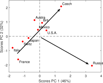
(a) Score plot

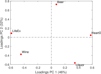
(b) Loading plot

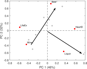
(c) Biplot

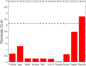
(d) Residuals: Q-statistic and control limits (95% and 99%)

Figure 1: PCA plots for the Wine data set.

We decompose the matrix of data into scores and loadings with two PCs, which represent 78% of the variance of the data. The variance is a measure of the patterns of change within the data. This means that the first 2 PCs contain almost 4/5 of the total patterns of change, and we can display all this information in a reduced number of plots.

The first plot (Figure 1(a)) is a score plot, which shows the distribution of the countries. In this plot we observe two patterns, highlighted with the arrows. Most countries are displayed in a quasi-linear pattern from France to the Czech Republic. As second pattern, Russia is far from the rest of the countries, manifesting a singular content in its variables in comparison to other countries.

The loading plot (Figure 1(b)) shows how variables distribute in the first 2 PCs. PC 1, in the abscissa, is mainly modeling the negative relationship between life expectancy and heart disease. The types of alcohol are evenly distributed in the plot, forming an almost perfect equilateral triangle. This shows that a preference for one type of alcohol leads to a reduced consumption of the other two.

Combining both scores and loadings in a biplot (Figure 1(c)), we can infer inter-connections between countries and variables. The trend from France to the Czech Republic shows where countries lie in their preference between wine and beer. Given also that this trend is slightly leaning towards the right, the pattern suggests that the wine preference correlates in the data with a higher life expectancy. Finally, Russia is separated from the rest due to its preference for liqueur and higher incidence of heart attacks.

Previous conclusions amount to 78% of the patterns of change in the data. This means that there is still 22% of change/information we have not observed yet. Most often, when subsequent PCs do not contain relevant patterns, we look at the residuals as squared aggregates. For instance, the residuals can be observed as sum-of-squares in the observations (or variables). The residual plot in Figure 1(d) shows there is more to understand about Mexico and Japan than what we observed in the first 2 PCs. Looking at the third PC (not shown), we can infer that mainly Mexico but also Japan have lower values in all variables, pattern that could not be seen in the first 2 PCs.

The matrix factorization in PCA can be extremely useful to understand data sets of high dimensionality, with up to thousands of variables or even more. Data interaction is also central in matrix factorization, due to its reduced computational burden: we can create a specific model to study in detail any pattern we find, or we can discard the data in a pattern in order to find new and more subtle patterns, an operation typically referred to as model update.

II-B MSNM for Interpretable Anomaly Detection

MSNM is an extension of the Multivariate Statistical Process Control developed in the past century, and originally inspired by the pioneering work in industrial quality control by Walter Andrew Shewhart [15]. MSNM is based on the PCA analysis of network data (traffic, logs, etc.), previously codified as interpretable counters. As part of statistical theory, interpretation has been a major cornerstone of MSNM.

MSNM handles the high-dimensional network data with PCA. From the scores and residuals in PCA, the data is further compressed in a pair of statistics, the D-statistic (D-st) and Q-statistic (Q-st), that represent the normality level of an observation in the model and residual sub-spaces of PCA, respectively. Upper control limits (UCLs, thresholds) are defined for each statistic to facilitate the detection of anomalies [15]. UCLs leave below-normal observations with a certain confidence level, e.g., $99\%$. An anomaly is detected if either its D-statistic or its Q-statistic exceed the corresponding control limit.

The D-statistic and the Q-statistic for observation $n$ are computed with the following equations:

$$D_{n}=\mathbf{t}_{n}\cdot(\Sigma_{T})^{-1}\cdot\mathbf{t}^{t}_{n}$$ (2)

$$Q_{n}=\mathbf{e}_{n}\cdot\mathbf{e}^{t}_{n}$$ (3)

where $\mathbf{t}_{n}$ is a $1\times A$ vector with the scores for observation $n$, $\mathbf{e}_{n}$ is a $1\times M$ vector with the residuals, and $\Sigma_{T}$ represents the covariance matrix of the scores. In order to detect anomalies, the number of PCs to use has to be determined. There are many methods to aid in that decision [16, 23].

Once an anomaly is detected, its interpretation is necessary for root cause analysis. Interpretation of anomalies in MSNM can be done following different diagnostic approaches [24, 25], but all of them amount to identifying a subset of variables associated with the specific anomaly. Generally speaking, diagnostic plots are plots where the contribution of the set of variables to a single statistic (D-st or Q-st) can be inspected.

Let us come back to the example of Figure 1(d). The Q-statistic for Mexico exceeds the control limit at 95% confidence level. An oMEDA diagnosis plot [26] is shown in Figure 2, with one bar per variable in the data. Since all bars are negative, we can conclude that Mexico has a lower value than the average country in all variables. This observation can be confirmed in Table I.

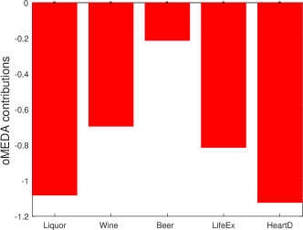
Figure 2: OMEDA diagnosis plot for Mexico for the Wine data set.

III Multivariate Big Data Analysis

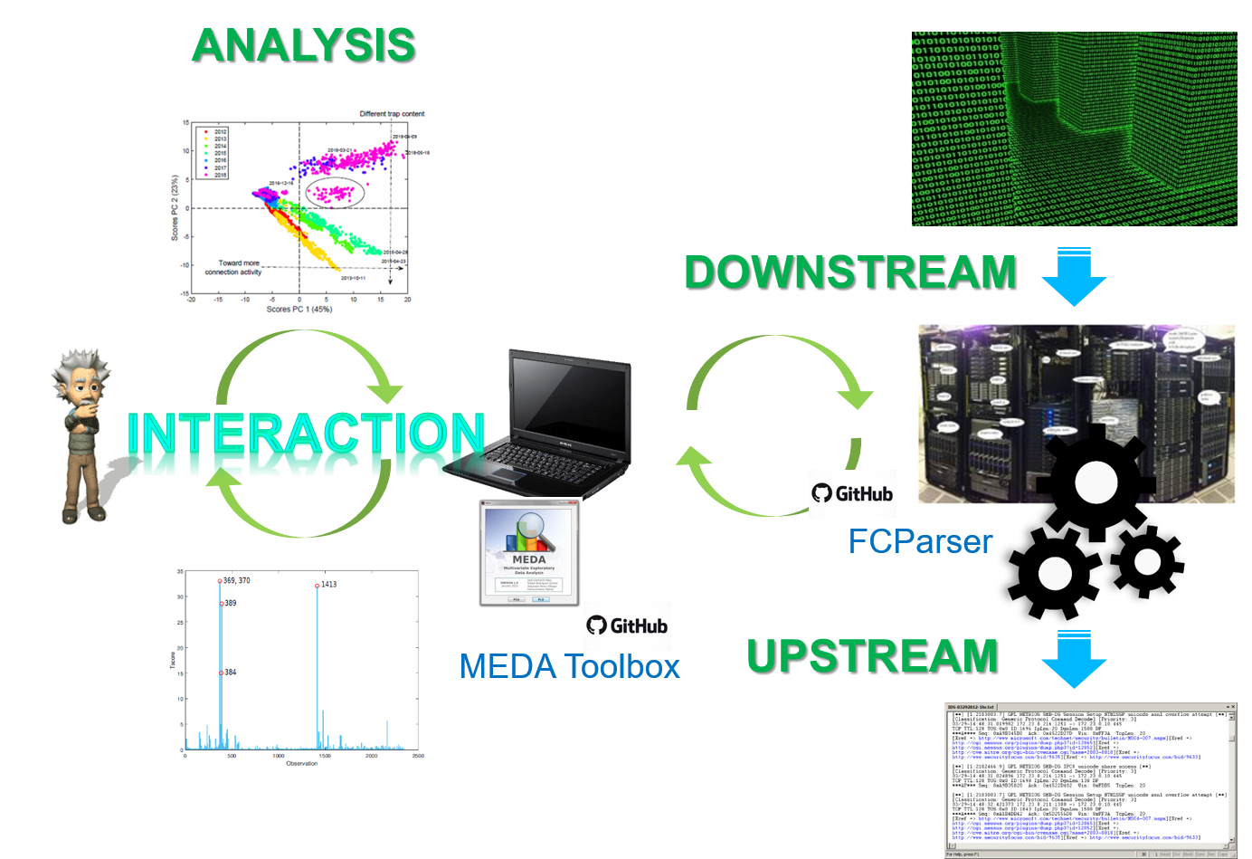
Figure 3: MBDA diagram.

The MBDA approach is depicted in Figure 3. It consists of three stages: downstream, analysis and upstream:

• In the downstream stage, we transform the Big Data input stream, coming from structured and/or unstructured sources, into time-resolved counters. The input stream is the data collected from the network (e.g., through a Security Information and Event Management system): typically a massive amount of logs and messages stored in a collector, potentially including different sources like network traffic, routing logs, SNMP, etc. [27]. We transform this data into a compressed form we refer to as the feature data. If several sources of data are considered, the features of the different sources of data are combined into a single feature data stream [15].

• In the analysis module, we visualize the feature data to identify anomalies in time using PCA and MSNM. For each anomaly, we find the associated features with a diagnosis plot, which provides a fast first hint to understand its root causes. The output of this second stage is a list of anomalies identified in time and the associated features.

• De-parsing: Using both detection and diagnosis information, we identify the original raw data records out of the massive input data that are related to the anomalies. This list of records allows a more detailed diagnosis, providing information about specific IPs, ports, etc. involved in the anomaly. The original MBDA paper [12] reports an accuracy above $0.99$ in presenting anomalous records, drastically reducing the amount of information to inspect by the human operator.

MBDA makes use of two open software packages available on Github: the MEDA Toolbox [28, 29] and the FCParser [30]. The FCParser is a Python tool for the parsing of both structured and unstructured logs. The MEDA Toolbox is a Matlab/Octave toolset for multivariate analysis and data visualization. The FCParser is used in the downstream and upstream modules, potentially on top of a computer cluster with enough computing power to handle the Big Data stream. The MEDA Toolbox is used in the analysis module in a regular computer, simplifying the interactive analysis by the human operator.

Basically, the downstream module transforms a Big Data stream into a manageable feature data set, that can be analyzed interactively in a traditional computer with multivariate analysis tools. Any interesting pattern found during the analysis can then be contrasted with the raw data thanks to the upstream module. Following this approach, we retain the interpretability and interactive nature of multivariate methods for the analysis of Big Data streams. These characteristics constitute a major advantage of MBDA over other Big Data methodologies, in particular black-box models.

III-A Feature-as-a-counter parsing

In the downstream stage, network logs are transformed into feature data. MBDA makes use of the feature-as-a-counter (FaaC) approach [7], described below.

In FaaC, each feature contains the number of times a given event takes place during a pre-defined time interval. Examples of suitable features are the counts of a given word in a log or the number of traffic flows with given destination port in a Netflow file. This flexible feature definition makes it possible to integrate, in a suitable way, most sources of information.

To implement the FaaC, the FCParser defines variables and features. Variables represent general entities in the raw data. In the previous two examples, the variables would be word and destination port. The features are defined for a specific value or regular expression of a variable. Examples of features would be word=‘food’ and destination port=‘80’. This representation in variables and features has the relevant advantage that allows for the definition of default features, e.g., word=$<$ANY_OTHER$>$, useful to count the instances of a variable that have not been considered in another feature.

Variables and features are defined using regular expressions in configuration files, where we also set the time resolution of the parsing. Each configuration file typically contains several variables and several features per variable. The FCParser applies this configuration to the data to compute a feature vector for each interval of time present in the original data. This operation is done using a multi-threading configuration to speed-up computation. By selecting the time resolution and the features, we define the trade-off between level of detail and compression. Defining more features and/or using a lower time resolution result in more detail, while defining fewer features and/or using a higher time resolution lead to more compression.

An example of the FaaC approach over a Simple Network Management Protocol (SNMP) trap of the second case study considered in this work can be found in Supplementary Materials.

IV Feature Learning in the Downstream Stage

MBDA relies on the definition of the features in the configuration files of the FCParser. To write such configuration files, the analyst needs to get familiarized with the data. Unfortunately, in a practical Big Data problem like the ones under analysis, the data capture is simply too massive for direct inspection. If we want to obtain a good description of the content, we may apply an automatic feature-derivation technique. The definition of this technique is not straightforward, since it needs to be consistent with the subsequent multivariate analysis, so that we maximize compression while retaining the interpretability required for anomaly detection and root cause analysis. There are two basic properties we would like to have in the learning procedure in consistency with PCA and MSNM: i) the main sources of variance (patterns of change within the data) need to be captured, and ii) uncommon characteristics with low variance should also be modeled somehow, in a summary of residual information.

We developed a learning algorithm to automatically identify a list of common FaaC features in a Big Data set, and included it in the FCParser repository at Github with the name fclearner.py. The learning algorithm is depicted in Algorithm 1. It takes as input a data set and a configuration file with the regular expressions of the variables. The goal is to learn features, that is, specific values that meet any of those regular expressions, with a local and global prevalence in the data above user-defined thresholds in the input configuration file, $T_{l}$ and $T_{g}$, respectively. The prevalence is defined as the portion of log entries where the feature appears in the raw data. The local prevalence threshold is applied over the time interval defined in the parsing, while the global prevalence is defined over the entire dataset.

Both local and global thresholds are complementary and need to be satisfied for a feature to be selected (learned). The local threshold $T_{l}$ needs to be satisfied at least in one time interval. The global $T_{g}$ needs to be satisfied in the complete data set. While in general $T_{l}$ may be lower than $T_{g}$, we may use higher values to speed-up computation. Satisfying both thresholds implies that any feature learned had to show a prevalence above $T_{l}$ in at least one interval and a global prevalence above $T_{g}$. That way, we learn those features that may be related to anomalous patterns in a handful of intervals, but with enough relevance to be considered a main source of change, meeting our first aforementioned requirement (i)). Those non-learned counters will still be integrated into the default features, so that we still have (arguably limited) observability of low variance patterns, meeting our second requirement (ii).

The learning algorithm works as follows. For each variable in the configuration file, the algorithm extracts its different features ($F_{j}^{1}$ to $F_{j}^{f}$) and the number of records in which they are found (counts $\#F_{j}^{1}$ to $\#F_{j}^{f}$) and store them in $\mathbf{P}_{j}$. The features which prevalence is above $T_{l}$ in at least one interval are included in list $\mathbf{F}_{j}$. At the last part, features with a global prevalence below $T_{g}$ or that are not in the list are discarded and their prevalence accumulated in the corresponding default feature ($F_{j}^{def}$) of the variable. Finally, the learning algorithm outputs all the features that satisfy both thresholds and the default features. The fclearner.py tool that implements this algorithm automatically transforms this output in a FCParser configuration file. In turn, this file can be used in the downstream stage of MBDA.

1

2

IN	PUT:
	$\mathbf{V}\leftarrow\{V_{1},...,V_{v}\}$: Regular expressions of variables
$\mathbf{D}\leftarrow\{D_{1},...,D_{d}\}$: Data files of disjoint time intervals
$T_{l}$: Local threshold
$T_{g}$: Global threshold
Ini	tialization:
	Set $C$ = 0: global counter of entries
Fo	r each variable $j$
	Set $\mathbf{P}_{j}=\emptyset$ : pairs of features and counts
Set $\mathbf{F}_{j}=\emptyset$ : list of features above threshold
Set $\#F_{j}^{def}$ = 0: count for default feature

3Al gorithm: Fo r each data file $D_{i}$ : parallelize at this point Fo r each time interval $D_{i}(t)$ in $D_{i}$ $C_{i}(t)\leftarrow count\_entries(D_{i}(t))$ $C\leftarrow C+C_{i}(t)$ Fo r each variable $j$ $\{(F_{j}^{1},\#F_{j}^{1})...,(F_{j}^{F},\#F_{j}^{F})\}\leftarrow Match(V_{j},D_{i}(t))$ $\mathbf{P}_{j}\leftarrow combine(\mathbf{P}_{j},\{(F_{j}^{1},\#F_{j}^{1})...,(F_{j}^{f},\#F_{j}^{F})\}$ ) Fo r $F_{j}^{f}$ in $\{F_{j}^{1}...,F_{j}^{F}\}$ If $(\#F_{j}^{f}/C_{i}(t))>T_{l}$ $\mathbf{F}_{j}\leftarrow\mathbf{F}_{j}\cup F_{j}^{f}$

4Fo r each variable $j$ Fo r $F_{j}^{f}$ in $\mathbf{P}_{j}$ If $(\#F_{j}^{f}/C)<T_{g}$ OR $F_{j}^{f}\not\in\mathbf{F}_{j}$ $\#F_{j}^{def}\leftarrow\#F_{j}^{def}+\#F_{j}^{i}$ $\mathbf{P}_{j}\leftarrow discard(\mathbf{P}_{j},(F_{j}^{i},\#F_{j}^{i})$)

5OUT PUT: $\mathbf{P}_{j}$ for all variables

6

Algorithm 1 Pseudocode for the learning algorithm.

V Materials & Methods

Below we describe the experimental case studies and the computational architecture used.

V-A The UGR’16 Case Study

The UGR’16 dataset [13] includes Netflow traffic flows captured in a ISP between March and June of 2016. In addition, another capture was made between July and August of 2016, including some controlled attacks launched to obtain a test dataset for validation of anomaly detection algorithms. To do this, twenty five virtual machines were deployed within one of the ISP sub-networks. Five of these machines attacked the other twenty. The type of attacks were: Denial of Service (DOS), port scanning in two modalities: either from one attacking machine to one victim machine (SCAN11) or from four attacking machines to four victim machines (SCAN44), and botnet traffic (NERISBOTNET). These attacks were launched during twelve days in different periods of time, following either planned or random scheduling, and with real background traffic. The flows of the dataset were labelled indicating if they were “background” (regarded as legitimate flows), or “anomalies” (identified as non-legitimate flows). The general characteristics of the dataset are provided in Table II.

TABLE II: Characteristics of the calibration and the test sets in UGR’16.

Feature Training Test Capture start 10:47h 03/18/2016 13:38h 07/27/2016 Capture end 18:27h 06/26/2016 09:27h 08/29/2016 Attacks start N/A 00:00h 07/28/2016 Attacks end N/A 12:00h 08/09/2016 Number of files 17 6 Size (compressed) 181GB 55GB # Connections $\approx$ 13,000M $\approx$ 3,900M

The UGR’16 data set was used to evaluate MBDA in its original work [12]. This application of MBDA, following a completely unsupervised anomaly detection approach, showed high performance in the detection of attacks with exception to the NERISBOTNET. Later, the detection performance was improved by using a semi-supervised extension of MBDA [31] based on Partial Least Squares (PLS) [32][33]. More recently, we showed that better performance than using semi-supervised methods can yet be achieved by properly performing outlier isolation in the background traffic [34]. Importantly, comparing MBDA to the One-Class Support Vector Machine (OCSVM), a widely used black-box anomaly detection approach, we found that outlier isolation impacts by far more than the specific anomaly detection method. We will benchmark the performance of the feature learning approach proposed in this paper against all these previous results.

Intensive Big Data analysis requires a parallel computer. We used a multi-GPU DGX-1 server with dual 20-core processors (80 threads) and 512GB RAM. Python scripts using the FCParser run on top of the parallel hardware as grid jobs. The paralellization of the downstream phase, from learning to parsing, is straightforward. We can split data in parallel jobs in agreement with the data file partition (see Algorithm 1), and the result is simply appended. This approach can also be applied in the upstream phase. The analysis stage was performed with the MEDA Toolbox in a regular laptop.

V-B The Dartmouth Wi-Fi network Case Study

Dartmouth College has a compact campus with over 200 buildings on 200 acres. The original evolution of the network is documented in the series of early papers [35, 36, 14]. The number of students, staff, and academic faculty reached near 6,500, 3,300 and 1,000, respectively, at the end of 2018, and the number of Access Points (APs) was above 3,000. Researchers at Dartmouth have been capturing data about the usage of the network for many years, providing a perfect case study for tools like MBDA.

In this paper we analyze a data capture containing the connections of users to the network in the seven years: from 2012 to 2018 [14]. This data contains Simple Network Management Protocol (SNMP) traps [37] sent from wireless controllers to a collector. The capture reveals the statistics in Table III. The data set contains a total of 5 Billion traps and 7 TB of data. A total of 38K authenticated users and an undetermined number of non-authenticated users have been connected to the network in the last seven years, using 600K devices. The network infrastructure supports several SSIDs, primarily Dartmouth Secure, the WPA2-Enterprise authenticated college network, Dartmouth Public, a public-access network, and eduroam, the world-wide roaming network for educational institutions [38]. Dartmouth Secure was entirely replaced by eduroam in the final months of the capture.

TABLE III: Details of the SNMP trap capture at Dartmouth College.

Statistic	Number
Capture period	Jan 1st 2012 - Dec 31st 2018
	(2556 days)
log entries (SNMP traps)	5 Billion
Data Size (raw)	7 TB
Access points	3,330
Authenticated Users	38,096
Stations	624,903
SSIDs	20

We used the Anthill Compute Cluster hosted by the Computer Science Department at Dartmouth for both the downstream and the upstream phase. Again, the analysis stage was performed with the MEDA Toolbox in a regular laptop.

VI UGR’16

Let us start with the application of the MBDA pipeline in the first case study. Our goal in this case is to automatically identify the attacks in the capture.

VI-A Downstream

VI-A1 Feature learning

We can think of at least two alternative ways to assess our approach for feature learning with the UGR’16 data set. One intuitive approach would be to learn the most prevalent features of background traffic in the training dataset, and then apply them for the detection of the attacks in the test set. This approach would render a purely unsupervised MBDA, equivalent to the work in [12]. Unfortunately, the background traffic also contains unlabeled anomalies and real attacks, and the evaluation based only in the artificial attacks may not be conclusive [34]. An alternative and arguably more objective option is to learn the features from part of the flows corresponding to the artificial attacks themselves, and assess if they provide an improved performance in the detection of the remaining flows of those attacks. This is the choice we take in the paper, which corresponds to a semi-supervised MBDA approach similar to the one in [31]. In a practical situation, the analyst would apply this approach when she wants to optimize the anomaly detector for specific (common) attacks. Still, given the unsupervised nature of the core of MBDA, MSNM, we retain the ability to detect unknown attacks.

In agreement with the semi-supervised version of MBDA in [31], we performed the feature learning on the raw files of the attacks corresponding to the first third of the test dataset, i.e., the first 4 days of attacks. The learning algorithm fclearner.py was launched in parallel in 24 processing jobs, one per hour in the day. The sampling interval, consistently with previous work, is set to 1 minute, and we set $T_{l}$ = 0.01 and $T_{g}$ = 0.001. Input variables were the source and destination port, the protocol and the tcp flags. Given the Netflow data is structured, the regular expressions of the variables are simply the location of the variable in the entries of the csv file with the raw dataset. The learning process resulted in a total of 396 features, most of them related to individual ports, and approximately 3 times the number of features in previous papers (134 manually selected features) [12, 31, 34]. We also considered a second set of learned features obtained for $T_{l}=T_{g}$ = 0.01, which resulted in a subset of the first set with a total of only 17 features. The whole learning process using the parallel hardware took 33 hours.

VI-A2 Parsing

We use FCParser to generate feature vectors with two variants of configuration files learned from the data: with 396 and 17 features, respectively. In agreement with the learning phase, we consider feature vectors for intervals of one minute. This generates a total of approx. 160K observations of 396/17 features, which can be handled with the Big Data version of the MEDA Toolbox in a regular computer [12]. Recall that we can vary the level of detail by using different time resolutions: if we use 1 hour intervals rather than 1 minute intervals, the number of observations would be reduced 60-fold to approx. 2,7K, but the resolution of detection would also be reduced.

The parsing was parallelized again in 24 processing jobs, one per hour in the day, and the whole process took 20 days. While this is a lengthy process, considering that the trace corresponds to 4 months of data, we can conclude that the parsing approach can be implemented in real time. In any case, this time can be reduced using a larger computer and properly arranging the input data for parallelization (see Algorithm 1). The resulting feature data is available on request from the authors.

VI-B Analysis

We focus on the ability of MBDA to identify the attacks in the part of the test set not used for the feature learning, that is, the last 8 days. To benchmark the anomaly detection performance with previous results, we compute the false positive rate (FPR) and true positive rate (TPR) of detection, and in turn the Receiver Operating Characteristic (ROC) curves, that shows the evolution of the TPR versus the FPR for different values of the anomaly detection threshold. A practical way to compare several ROC curves is with the Area Under the Curve (AUC), a scalar that quantifies the quality of the anomaly detector. The anomaly detector should present an AUC as close to 1 as possible, while an AUC around 0.5 corresponds to a random classifier.

Figure 4 shows the comparison of a number of different MBDA variants (see also Table IV), including:

• MBDA: The original, unsupervised approach [12] trained with the complete training dataset using manually selected features.

• MBDA Opt: The semi-supervised extension of MBDA [31] trained with the complete training dataset using manually selected features and optimized with Partial Least Squares (PLS) using the attacks of the first four days of the testset.

• MBDA WoJ: The unsupervised MBDA with manually selected features trained without June, where an anomaly with a similar pattern as a botnet was found [34].

• MBDA FL_0.001: The semi-supervised MBDA trained with the complete training dataset and with the 396 features learned for $T_{g}$ = 0.001 using the attacks of the first four days of the testset.

• MBDA FL_0.01: The semi-supervised MBDA trained with the complete training dataset and with the 17 features learned for $T_{g}$ = 0.01 using the attacks of the first four days of the testset.

• MBDA WoJ FL_0.01: The semi-supervised MBDA trained without June and with the 17 features learned for $T_{g}$ = 0.01 using the attacks of the first four days of the testset.

TABLE IV: MBDA variants under study.

Name Type Features June in training data MBDA unsupervised manual Yes MBDA Opt semi-supervised manual Yes MBDA WoJ unsupervised manual No MBDA FL_0.001 semi-supervised learned ($T_{g}$ = 0.001) Yes MBDA FL_0.01 semi-supervised learned ($T_{g}$ = 0.01) Yes MBDA WoJ FL_0.01 semi-supervised learned ($T_{g}$ = 0.01) No

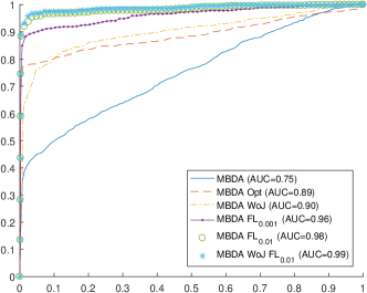
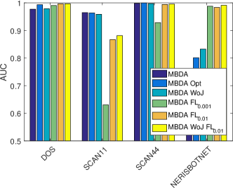
Figure 4: ROC curves (a) and attack-type based AUC results (b) for a set of different solutions based on MBDA.

Figure 4(a) presents the general ROC curves, obtained for the four types of attacks, and Figure 4(b) represents the AUCs per attack type. Our proposal for feature learning generally outperforms other methods based on manually selected features. We can see that the improvements are mainly on NERISBOTNET attacks, while the performance for SCAN attacks is generally better for versions of MBDA with manually selected features.

We can obtain more information about the root causes for aforementioned performance differences among the models when detecting specific attacks. For that purpose, we use the approach presented in [34] that combines oMEDA diagnosis plots (in particular, the full-rank version of oMEDA also referred to as Univariate-Squared (U-Squared) [25]), univariate box plots and t-tests for statistical inference. We compare MBDA Opt and MBDA FL_0.01 as representatives of models with manual features and learned features, respectively, since both are semi-supervised and trained with the complete training dataset.

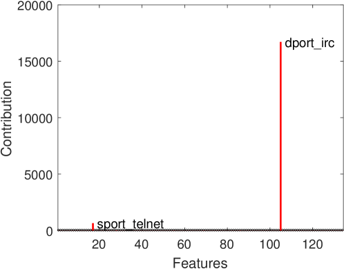
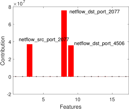
Figure 5: Profile of detection of NERISBOTNET attacks with MBDA Opt (a) and MBDA FL_0.01 (b) using oMEDA.

The diagnosis plots for NERISBOTNET attacks are shown in Figure 5. MBDA Opt emphasizes irc and telnet ports, while MBDA FL_0.01 focuses on ports 2077 and 4506. All selected features yield statistically significant differences between background traffic and NERISBOTNET attacks, as illustrated in Figure 6. However, according to AUC results, learned features provide a more powerful detection.

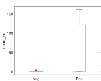
(a) Ttest $\mathbf{p_{-}value<0.01}$

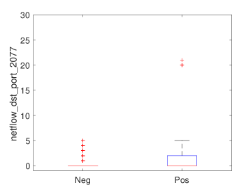
(b) Ttest $\mathbf{p_{-}value<0.01}$

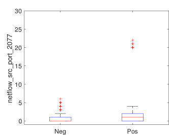
(c) Ttest $\mathbf{p_{-}value<0.01}$

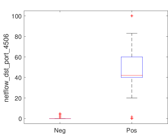
(d) Ttest $\mathbf{p_{-}value<0.01}$

Figure 6: Boxplots and ttests of selected features in background traffic (Negative) versus NERISBOTNET traffic (Positive).

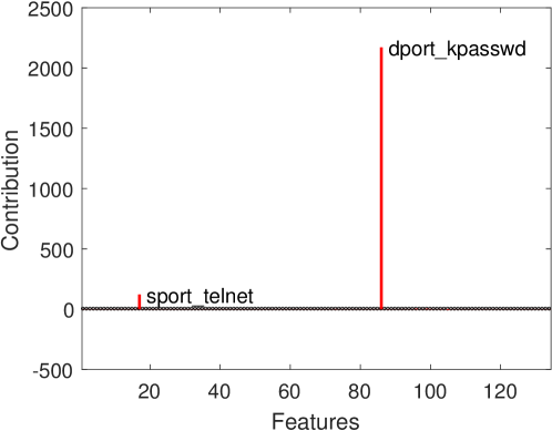
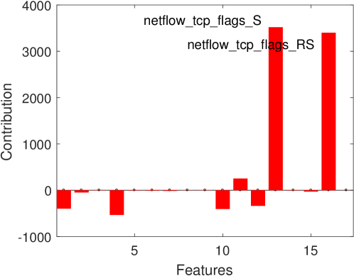
Figure 7: Profile of detection of SCAN11 attacks with MBDA Opt (a) and MBDA FL_0.01 (b) using oMEDA.

We repeat the same procedure for SCAN11 attacks, shown in Figures 7 and 8. MBDA Opt emphasizes kpasswd and telnet ports, while MBDA FL_0.01 focuses on the TCP flags, in particular Sync and the combination of Reset and Sync. In this case, the manual selection of features provides a more powerful detection in terms of AUC. However, neither pattern of detection is perfect: in SCAN attacks, the attacker sends probing messages to find open ports, and does that for a large number of different ports. MBDA Opt only detects the attack because there is one single port of those tested, kpasswd, with negligible background traffic, but the diagnosis does not reflect the true pattern of attack. MBDA FL_0.01 provides limited performance because the learning approach based on prevalence and counting features cannot capture the pattern of the attack. Future work may look at different learning loss functions other than prevalence and/or alternative definitions of features that capture distributional information of a variable, like the number of different ports in a time interval.

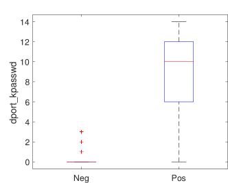
(a) Ttest $\mathbf{p_{-}value<0.01}$

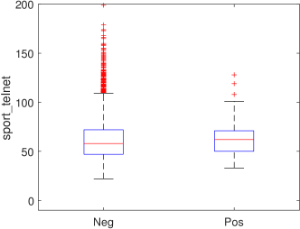
(b) Ttest $\mathbf{p_{-}value<0.01}$

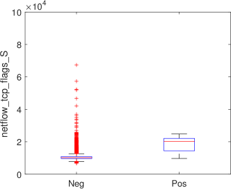
(c) Ttest $\mathbf{p_{-}value<0.01}$

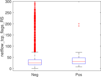
(d) Ttest $p_{-}value=0.83$

Figure 8: Boxplots and t-tests of selected features in background traffic (Negative) versus SCAN11 traffic (Positive).

VI-C Upstream

The previous analysis compared the accuracy of detection at time interval (1 minute) level. As an illustrative example of the upstream step, we compare here the accuracy of detection of the NERISBOTNET attack at flow-level by MBDA Opt and MBDA FL_0.01. Results are presented in Table V in terms of the number of true positives (TP) and negatives (TN), the number of false positives (FP) and negatives (FN), the accuracy ((TP+TN)/Total) and the False Discovery Rate (FDR = FP /(TP+FP)). While accuracy levels are close to 1.00, like those reported earlier [12], the FDR is a more relevant statistic to assess the difficulty in the process of root cause analysis. The FDR gives us an estimate of the relative number of false alarms an analyst will have to face in the process of alarm validation. In the example, we can see that the MBDA based on feature learning reduces the relative number of false alarms to only 1.8%, which is a competitive statistic and much lower that the one using manual features.

TABLE V: Comparison of MBDA Opt and MBDA FL_0.01 in the upstream step in the detection of the NERISBOTNET attack. We present the number of true positives (TP) and negatives (TN), the number of false positives (FP) and negatives (FN), the accuracy ((TP+TN)/Total) and the False Discovery Rate (FDR = FP /(TP+FP)). The total number of flows in the test data (the part used for performance evaluation, that is, the last 8 days) is 1,074,221,524, and the number of attack flows in the same data is 1,074,493 (0.1% of the total).

Method	TP	TN	FP	FN	Accuracy	FDR
MBDA Opt	33,613	1,073,101,984	45,047	1,040,880	$\approx 1.00$	0.570
MBDA FL0.01	61,261	1,073,145,928	1,103	1,013,232	$\approx 1.00$	0.018

VII Dartmouth Wi-Fi

Let us move on to the analysis of the Dartmouth Wi-Fi capture. Our goal here is to visualize and understand the main factors of variance in the connection data.

VII-A Downstream

VII-A1 Feature learning

TABLE VI: First 10 SNMP OIDs with more prevalence in the data. CLAM refers to CISCO-LWAPP-AP-MIB, AWM to AIRESPACE-WIRELESS-MIB and CLDCM to CISCO-LWAPP-DOT11-CLIENT-MIB.

Label	Type	Presence
CLAM::cLApDot11IfSlotId	OID	0.45
AWM::bsnAPName	OID	0.41
AWM::bsnStationMacAddress	OID	0.39
AWM::bsnStationAPIfSlotId	OID	0.39
AWM::bsnStationAPMacAddr	OID	0.39
AWM::bsnStationUserName	OID	0.39
CLAM::cLApName	OID	0.36
CLDCM::cldcClientMacAddress	OID	0.22
CLDCM::cldcApMacAddress	OID	0.22
AWM::bsnDot11StationAssociate	TT	0.20

We performed the learning strategy in two steps to identify high variance features in the Wi-Fi data. First, the learning algorithm fclearning.py was launched in parallel in 2556 processing jobs, each one for a different day in the capture, using a sampling interval of 1 day and a threshold values $T_{l}=0.05$ and $T_{g}=0.01$. Input variables were the regular expressions for a SNMP object identifier (OID) and for the trap type (TT) (see Supplementary Materials for more detail). The output is 2556 configuration files, one per day, with the set of most prevalent OIDs and TTs in each day. That way, we learn as features all those OIDs or TTs with a daily prevalence above the 5% in at least one day and a total prevalence above 1%. This resulted in a total of 90 features, including prevalent OIDs, TTs and default features. The ten most prevalent features are shown in Table VI, where we make the distinction between OIDs representing trap types (TTs) and the rest.

The whole learning process using the parallel hardware and multi-threading (4 threads per processor) took 12 hours, during which a maximum of 150 jobs were processed in parallel. This means that the processing time could be further reduced 17-fold using a larger computer cluster, where as many as 2556 jobs could be run in parallel.

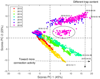
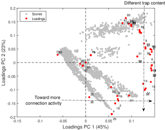
Figure 9: PCA scores and loadings for PC1 vs PC2.

VII-A2 Parsing

We use the FCParser to generate the feature vectors with the aforementioned configuration file learned from the data. In agreement with the learning phase, we consider feature vectors for intervals of one day. To the set of 90 learning features, we added the total number of traps and OIDs per day. This results in a compression of the data from 7TB to less than 1MB, yielding 2556 observations (days) of 92 features each in matrix $\mathbf{X}$. The compression conveniently transforms a Big Data set into a handleable data set in a common computer. Again, we can vary the level of detail by using different time resolutions or number of features.

The parsing was parallelized in 2556 processing jobs, one per day, and the whole process using the Anthill Computer Cluster and multi-threading (with a maximum of 150 jobs) took 15 hours. The resulting feature data is available on request from the authors.

VII-B Analysis

VII-B1 Analysis with PCA

Figure 9 depicts the plots corresponding to the first two PCs in matrix $\mathbf{X}$ (refer to Supplementary Materials for other patterns found in subsequent PCs). Recall that matrix $\mathbf{X}$ contains 2556 rows, representing days of the capture, and 92 features. We present the score plot at the left of the figure and a bi-plot at the right. In the score plot, points represent the 2556 days of the data capture and are colored according to the year. In the bi-plot, (red) points represent the 92 features and the (gray) shadow represent the scores.

The first two PCs represent 68% (45% + 23%) of the variance in the data. Because variance is a measure of the degree of change within the data set, these two PCs show the main patterns of change in $\mathbf{X}$. As a matter of fact, a variance of $68\%$ roughly indicates that only 1/3 of the patterns of change in the data is missing in this plot, giving an idea of how powerful PCA is for visualization.

The score plot at Figure 9(a) shows that the dots (days) with different colors are in different locations. This means that they are different in content, from which follows that there are large differences in prevalence of OIDs in different years.

To interpret the bi-plot at Figure 9(b), recall that the location of an observation (a day) will approach more the location of a feature (which represents counts of a specific OID) as the value of that feature increases in the observation. Thus, days with a large content on specific OIDs will be located closer in the plot to the loading representing that OID. The bi-plot shows that a large majority of the features are located far from the center of coordinates towards the right side. Therefore, any day toward the right in the score plot will have a generally higher content of OIDs. Thus, as we traverse from left to right in the score plot, the days will have more connection activity. Busy periods are represented towards the far right of the plot, and vacations are clustered to the left, and we could say that the first PC (the horizontal direction in the score and loading plots) represents the general activity in the network. We annotated this in both plots using a horizontal arrow.

The bi-plot in Figure 9(b) also shows that the variables are distributed from the bottom to top, and we see a similar distribution for the different years in the score plot: the first two years are in the bottom and the last two in the top, with middle years in between. We also see a separated cluster of days in 2018, highlighted with a circle. A closer look reveals that all the days in the cluster belong to the period from September to November, when eduroam replaced Dartmouth Secure. The vertical pattern in the loading and score plots shows that the distribution of traps has changed across the years: days towards the top have a higher content of traps and OIDs represented by the features in the top and less of those in the bottom, and vice-versa. Again, we annotated this in the score plot and the bi-plot using a vertical arrow. Questioned about this difference, the network operators replied that there was an update in the controllers’ software, which changed the types of SNMP traps that were collected. This variability in traps for different temporal periods makes the analysis of the data a real challenge. It may also go unnoticed if we do not use feature learning, since to determine features manually we can only screen limited portions of the massive data, and this operation would likely miss the changing pattern of OIDs.

Regarding processing burden, the analysis performed in this section is completely interactive in a regular computer, meaning that the time to obtain each of the plots is on the order of seconds.

VII-B2 Analysis with MSNM

TABLE VII: Pre-diagnosis of the excursions of 2013 and 2017 with oMEDA.

Timestamps	Features selected
2013-12-14 – 2013-12-16	bsnDot11StationAuthenticateFail, bsnAuthenticationFailure, bsnDot11StationAssociateFail,
	bsnStationReasonCode, bsnAuthFailureUserType, bsnAuthFailureUserName
2017-10-16 – 2017-10-30	ciscoLwappApIfUpNotify, ciscoLwappApIfDownNotify
	cLApAdminStatus, cLApSysMacAddress, cLApPortNumber

After the inspection of score and loading plots, one can visualize a summary of the whole data distribution in one single plot using MSNM: a scatter plot of the observations in terms of the D-statistic and the Q-statistic. The MSNM plot for the Wi-Fi data is shown in Figure 10. Anomalies are expected to surpass any of the two control limits: the vertical one for the D-statistic or the horizontal one for the Q-statistic. This plot is optimized for anomaly detection. Note that with only one visualization, the operator can identify the main patterns of change in 7TB of data. Clearly, in the plot we miss other details, like yearly and seasonal patterns and the difference in trap contents. A main advantage of this plot is that it also includes residuals, containing the remaining 6% of the variance that is not accounted for in the six PCs (including those shown in the Supplementary Materials). The Q-statistic, which comprises a summary of the residuals, clearly identifies anomalies in 2012 and 2013, while the D-statistic finds several anomalous intervals in 2012 and 2017.

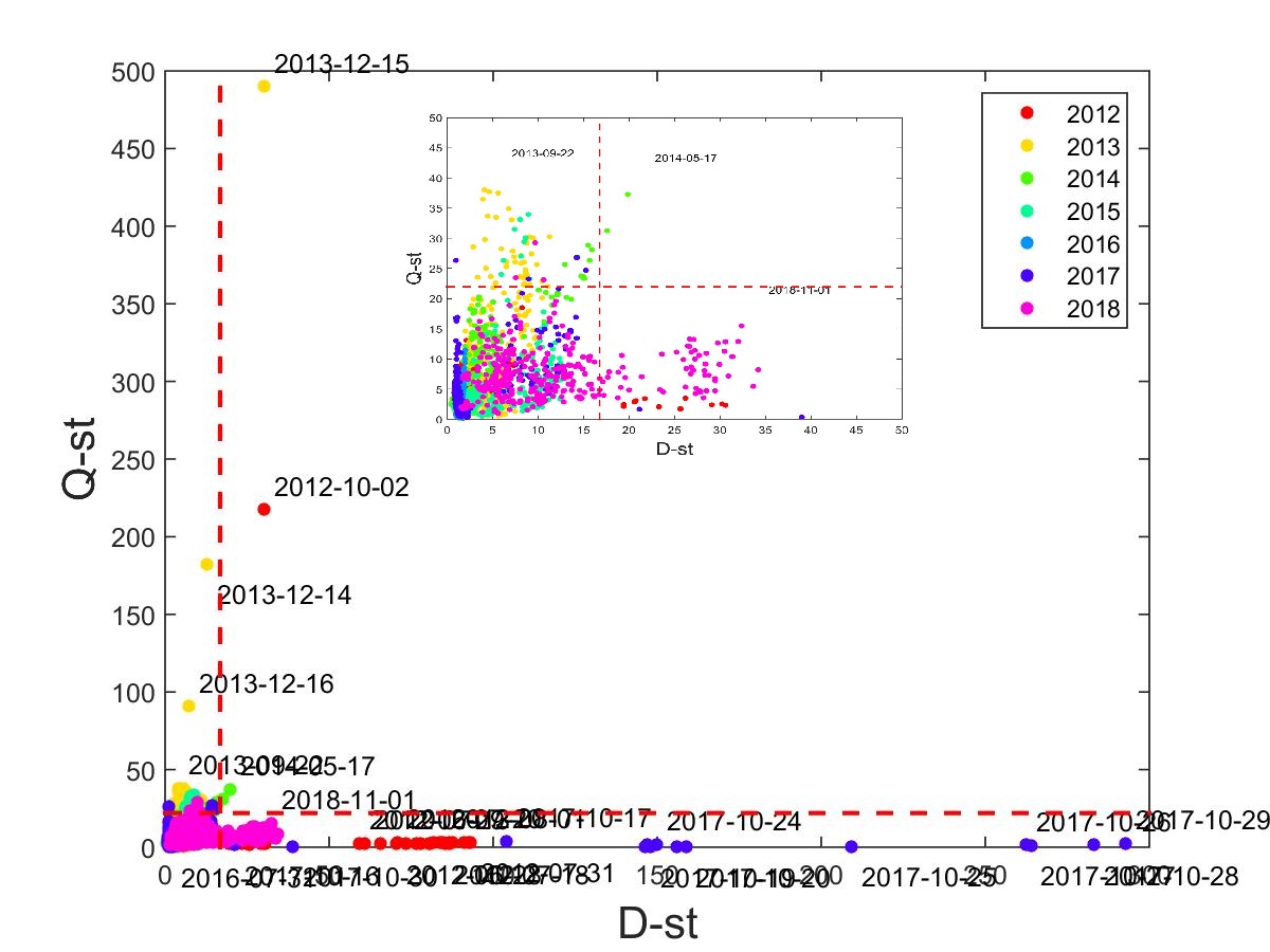
Figure 10: Multivariate Statistical Network Monitoring (MSNM) plot: D-statistic vs Q-statistic. At the top, zoomed image of the bottom left corner.

Note that the parsing (and thus of the learning process) has a principal impact in the visualization and anomaly detection of MBDA. For instance, we can detect anomalies (e.g., excursions) only at the day level when using one-day resolution. If we want to detect anomalies in other time resolutions, we can modify the parsing configuration and re-run the downstream stage. Furthermore, differences in OID content can only be directly visualized if we include features for those OIDs (recall default features will still represent such differences to a certain level). Therefore, learning features of high variance is paramount to obtaining accurate insights of the data distribution.

To illustrate the use of oMEDA in the diagnosis, we selected the anomalies in 2013 and 2017, which we found to be the main outliers in the Q-statistic and in the D-statistic, respectively. The plots are shown in Figure 11. The high bars identify the features that make the anomalous intervals different to the normal days. Each of the intervals are related to a different set of features. Table VII lists the specific features. We determined that the first anomaly (2013) is related to a large number of Authentication Fails, which in a subsequent analysis (not shown) we determined these fails were one order of magnitude higher than usual during the detected anomalous interval. The second anomaly (2017) is related to an unprecedentedly high number of re-starts of APs, two orders of magnitude higher than usual.

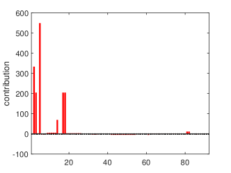
(a) Excursion in 2013

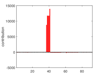
(b) Excursion in 2017

Figure 11: Pre-diagnosis of the anomalies in 2013 and 2017 with oMEDA.

As for 2018, the network operators did not have any records of these old anomalies, but they suggested that the second one could be related to the installation of a security patch after the publication of a vulnerability. Effectively, October 16th of 2017, the famous KRACK attack against WPA2 [39] and the corresponding patch was released to the public. Even if a restart is necessary after a patch installation, the number and duration (15 days) of the event is remarkable, evidencing that a major management problem took place that went unnoticed into the massive stream of SNMP traps.

Like the PCA analysis, the MSNM analysis is fully interactive and easily done in a regular computer.

VII-C Upstream

TABLE VIII: Deparsing of the anomalies of 2013 and 2017 with oMEDA.

Timestamps	log entries/tot	#APs	#Stations	#Users
2013-12-14 – 2013-12-16	5.4M/8.4M (64%)	824	595	103
2017-10-16 – 2017-10-30	19.0M/64.1M (30%)	1,376	0	0

We applied the upstream stage with the FCParser to the anomalies in 2013 and 2017 in the Wi-Fi data set. We parallelized the processing using the Anthill Computer Cluster and multi-threading (4 threads per processor), with as many parallel jobs as days in the excursions. The first anomaly took 30 minutes to be processed, and the second one 135 minutes. The output is a file per anomaly, containing the traps involved, which represent a subset of total set of traps in the corresponding periods of time. Table VIII provides some statistics of the deparsing. The human operator can use the output files to retrieve more information about the anomalies, like the main actors (APs, users, devices) involved.

VIII Conclusion

In this paper, we introduce feature learning in the Multivariate Big Data Analysis (MBDA), an interpretable data analysis tool optimized to analyze Big Data streams, for network monitoring. The application is concerned with the detection and diagnosis of anomalies in two real case studies: a Netflow trace from a TIER-3 ISP and a connection trace from a campus Wi-Fi network. The results illustrate that multivariate methods can bring light into massive data sets for network-monitoring purposes using interpretable feature learning.

The main advantages of the approach, illustrated through the paper, are the following:

• With MBDA, we can detect anomalies and other data patterns related to network operation that may go unnoticed otherwise due to the massive nature of network data. The paper illustrates several examples of those patterns. The detection is general in the sense that anomalies are detected without actually targeting them, so we do not require the user to pre-identify a set of potential failures.

• Thanks to the interpretability of multivariate models in the core of MBDA, we can also diagnose problems, so that potential root causes can be identified and problems can be troubleshooted faster.

• MBDA can run on parallel hardware to speed up computation. We analyzed 7TB of data in a little more than a day, and this can be reduced to a couple of hours in a high-throughput cluster.

• The MBDA data pipeline is designed so that the data analysis is partially done in a cluster of computers and in a regular computer. Long operations with raw, Big Data, are done in a cluster and provide as output a feature data set of limited size. These operations can be scheduled in non-busy periods of time and be fully automated. The network operator only needs to interact with the feature data to detect anomalies and diagnose them, and this can be done in real time in a regular computer. This approach combines the advantages of interactive models with the power of parallel processing.

• MBDA using feature learning is general framework for the extension of exploratory multivariate analysis to Big Data.

José Camacho José Camacho is Full Professor in the Department of Signal Theory, Telematics and Communication and head of the Computational Data Science Laboratory (CoDaS Lab), at the University of Granada, Spain. He holds a degree in Computer Science from the University of Granada (2003) and a Ph.D. from the Technical University of Valencia (2007), both in Spain. He worked as a post-doctoral fellow at the University of Girona, granted by the Juan de la Cierva program, and was a Fulbright fellow in 2018 at Dartmouth College, USA. His research interests include networkmetrics and intelligent communication systems, computational biology, knowledge discovery in Big Data and the development of new machine learning and statistical tools.

Katarzyna Wasielewska Katarzyna Wasielewska received MSc in computer science from the Faculty of Mathematics and Computer Science, Nicolaus Copernicus University in Torun (NCU), Poland, in 1999, and PhD in telecommunications from the Faculty of Telecommunication, Information Technology and Electrical Engineering, University of Science and Technology in Bydgoszcz (UTP), Poland, in 2014. She is Assistant Professor at the Institute of Applied Informatics, State University of Applied Sciences in Elblag, Poland. Currently, she is a Postdoctoral Researcher at the Department of Signal Theory, Telematics and Communication and the CoDaS Lab, University of Granada, Spain, granted by EU Marie Skodowska-Curie Actions Individual Fellowships program. Her research interests include computer communications, network traffic analysis, network security, multivariate analysis and machine learning. She worked 10 years as an ISP network administrator, and she is an active IEEE volunteer.

Rasmus Bro Rasmus Bro (born 1965) studied mathematics and analytical chemistry at the Technical University of Denmark and received his M.Sc. in 1994. In 1998 he obtained his Ph.D. in multiway analysis from the University of Amsterdam, The Netherlands. Since 1994 he has been employed at the Department of Food Science, at the University of Copenhagen, and in 2002 he was appointed full professor of chemometrics. He has had several stays abroad at research institutions in The Netherlands, Norway, France, and United States. Current research interests include chemometrics, multivariate calibration, multiway analysis, exploratory analysis, blind source separation, curve resolution, MATLAB programming.

David Kotz David Kotz is the Provost, and the Pat and John Rosenwald Professor in the Department of Computer Science, at Dartmouth College. He previously served as Associate Dean of the Faculty for the Sciences, as a Core Director at the Center for Technology and Behavioral Health, and as the Executive Director of the Institute for Security Technology Studies. His current research involves security and privacy in smart homes, and wireless networks. He has published over 250 refereed papers, obtained $89m in grant funding, and mentored over 100 research students and postdocs. He is an ACM Fellow, an IEEE Fellow, a 2008 Fulbright Fellow to India, a 2019 Visiting Professor at ETH Zürich, and an elected member of Phi Beta Kappa. He received his AB in Computer Science and Physics from Dartmouth in 1986, and his PhD in Computer Science from Duke University in 1991.

References

-
[1]
H. Song, F. Qin, P. Martinez-Julia, L. Ciavaglia, A. Wang,
Network
Telemetry Framework, Internet-Draft draft-ietf-opsawg-ntf-13, Internet
Engineering Task Force, work in Progress (Dec. 2021).
URL https://datatracker.ietf.org/doc/html/draft-ietf-opsawg-ntf-13 - [2] G. Pang, C. Shen, L. Cao, A. V. D. Hengel, Deep learning for anomaly detection: A review, ACM Computing Surveys (CSUR) 54 (2) (2021) 1–38.
- [3] C. Molnar, Interpretable Machine Learning, 2019, https://christophm.github.io/interpretable-ml-book/.
- [4] F. Doshi-Velez, B. Kim, Towards a rigorous science of interpretable machine learning, arXiv preprint arXiv:1702.08608 (2017).
- [5] C. Rudin, Stop explaining black box machine learning models for high stakes decisions and use interpretable models instead (2019). arXiv:1811.10154.
- [6] A. Ferrer, Latent structures-based multivariate statistical process control: A paradigm shift, Quality Engineering 26 (1) (2014) 72–91.
- [7] J. Camacho, G. Maciá-Fernández, J. Díaz-Verdejo, P. García-Teodoro, Tackling the Big Data 4 Vs for anomaly detection, in: Proceedings of IEEE INFOCOM, 2014, pp. 500–505. doi:10.1109/INFCOMW.2014.6849282.
- [8] J. Hernández-Méndez, F. Muñoz Leiva, J. Sánchez-Fernández, The influence of e-word-of-mouth on travel decision-making: consumer profiles, Current Issues in Tourism 1-14 (2013) 1–21. doi:10.1080/13683500.2013.802764.
- [9] I. Jolliffe, Principal component analysis, Springer Verlag, New York, 2002.
- [10] H. Zou, T. Hastie, R. Tibshirani, Sparse Principal Component Analysis, Journal of Computational and Graphical Statistics 15 (2) (2006) 265–286. arXiv:1205.0121v2, doi:10.1198/106186006X113430.
- [11] R. Bro, Multi-way analysis in the food industry - models, algorithms, and applications, Tech. rep., MRI, EPG and EMA, Proc ICSLP 2000 (1998).
- [12] J. Camacho, J. M. García-Giménez, N. M. Fuentes-García, G. Maciá-Fernández, Multivariate big data analysis for intrusion detection: 5 steps from the haystack to the needle, Computers & Security 87 (2019) 101603.
- [13] G. Maciá-Fernández, J. Camacho, R. Magán-Carrión, P. García-Teodoro, R. Therón, UGR‘16: A new dataset for the evaluation of cyclostationarity-based network IDSs, Computers & Security 73 (2018) 411–424.
- [14] J. Camacho, C. McDonald, R. Peterson, X. Zhou, D. Kotz, Longitudinal analysis of a campus wi-fi network, Computer Networks 170 (2020) 107103.
-
[15]
J. Camacho, A. Pérez-Villegas, P. García-Teodoro, G. Maciá-Fernández,
PCA-based
multivariate statistical network monitoring for anomaly detection, Computers
& Security 59 (2016) 118–137.
doi:10.1016/j.cose.2016.02.008.
URL http://www.sciencedirect.com/science/article/pii/S0167404816300116 - [16] J. Jackson, A User’s Guide to Principal Components, Wiley-Interscience, England, 2003.
- [17] J. V. Kresta, J. F. Macgregor, T. E. Marlin, Multivariate statistical monitoring of process operating performance, The Canadian Journal of Chemical Engineering 69 (1) (1991) 35–47. doi:10.1002/cjce.5450690105.
- [18] P. Nomikos, J. F. MacGregor, Monitoring batch processes using multiway principal component analysis, AIChE Journal 40 (8) (1994) 1361–1375. doi:10.1002/aic.690400809.
- [19] A. Ferrer, Multivariate statistical process control based on principal component analysis (MSPC-PCA): Some reflections and a case study in an autobody assembly process, Quality Engineering 19 (4) (2007) 311–325. doi:10.1080/08982110701621304.
- [20] K. Gabriel, The biplot graphic display of matrices with application to principal component analysis, Biometrika 58 (1971) 453–467.
- [21] Pls-toolbox, Newsweek 127 (4) (1996) 52.
- [22] B. Wise, N. Gallagher, R. Bro, J. Shaver, W. Windig, R. Koch, PLSToolbox 3.5 for use with Matlab, Eigenvector Research Inc., 2005.
-
[23]
E. Saccenti, J. Camacho,
Determining
the number of components in principal components analysis: A comparison of
statistical, crossvalidation and approximated methods, Chemometrics and
Intelligent Laboratory Systems 149, Part A (2015) 99–116.
doi:10.1016/j.chemolab.2015.10.006.
URL http://www.sciencedirect.com/science/article/pii/S0169743915002579 - [24] C. F. Alcala, S. J. Qin, Reconstruction-based contribution for process monitoring, Automatica 45 (7) (2009) 1593–1600.
-
[25]
M. Fuentes-García, G. Maciá-Fernández, J. Camacho,
Evaluation
of diagnosis methods in PCA-based multivariate statistical process
control, Chemometrics and Intelligent Laboratory Systems 172 (2018)
194–210.
doi:10.1016/j.chemolab.2017.12.008.
URL http://www.sciencedirect.com/science/article/pii/S0169743917302046 - [26] J. Camacho, Observation-based missing data methods for exploratory data analysis to unveil the connection between observations and variables in latent subspace models, Journal of Chemometrics 25 (11) (2011) 592–600.
- [27] M. Fuentes-García, J. Camacho, G. Maciá-Fernández, Present and future of network security monitoring, IEEE Access 9 (2021) 112744–112760. doi:10.1109/ACCESS.2021.3067106.
- [28] J. Camacho, A. Pérez-Villegas, R. A. Rodríguez-Gómez, E. Jiménez, Multivariate exploratory data analysis (MEDA) toolbox for Matlab, Chemometrics and Intelligent Laboratory Systems 143 (0) (2015) 49–57. doi:10.1016/j.chemolab.2015.02.016.
- [29] GitHub repository for the MEDA Toolbox, https://github.com/josecamachop/MEDA-Toolbox, accessed: 2018-09-30.
- [30] GitHub repository for the FCParser, https://github.com/josecamachop/FCParser, accessed: 2018-09-30.
- [31] J. Camacho, G. Maciá-Fernández, N. M. Fuentes-García, E. Saccenti, Semi-supervised multivariate statistical network monitoring for learning security threats, IEEE Transactions on Information Forensics and Security 14 (8) (2019) 2179–2189. doi:10.1109/TIFS.2019.2894358.
- [32] H. Martens, T. N. s, Multivariate Calibration, John Wiley & Sons, 1992.
- [33] P. Geladi, B. Kowalski, Partial least-squares regression: a tutorial, Analytica Chimica Acta 185 (1986) 1–17.
- [34]
- [35] D. Kotz, K. Essien, Analysis of a campus-wide wireless network, Wireless Networks 11 (1–2) (2005) 115–133. doi:10.1007/s11276-004-4750-0.
- [36] T. Henderson, D. Kotz, I. Abyzov, The changing usage of a mature campus-wide wireless network, Computer Networks 52 (14) (2008) 2690–2712. doi:10.1016/j.comnet.2008.05.003.
-
[37]
J. Case, M. Fedor, M. Schoffstall, J. Davin,
A Simple Network
Management Protocol (SNMP), RFC 1157, RFC Editor (May 1990).
URL https://www.rfc-editor.org/rfc/rfc1157.txt - [38] Eduroam: World wide education roaming for research & education, https://www.eduroam.org/, accessed: 2018-09-30.
-
[39]
M. Vanhoef, F. Piessens, Key
reinstallation attacks: Forcing nonce reuse in WPA2, in: Proceedings of
the ACM SIGSAC Conference on Computer and Communications Security, CCS ’17,
ACM, 2017, pp. 1313–1328.
doi:10.1145/3133956.3134027.
URL http://doi.acm.org/10.1145/3133956.3134027 - [40] A. D’Alconzo, I. Drago, A. Morichetta, M. Mellia, P. Casas, A survey on big data for network traffic monitoring and analysis, IEEE Transactions on Network and Service Management 16 (3) (2019) 800–813. doi:10.1109/TNSM.2019.2933358.
- [41] Q. Thai, C. Ordonez, O. Gnawali, Monitoring networks with queries evaluated by edge computing, in: 2020 IEEE International Conference on Big Data (Big Data), 2020, pp. 2223–2231. doi:10.1109/BigData50022.2020.9377998.
- [42] P. Khandait, N. Hubballi, B. Mazumdar, Efficient keyword matching for deep packet inspection based network traffic classification, in: 2020 International Conference on COMmunication Systems NETworkS (COMSNETS), IEEE, 2020, pp. 567–570. doi:10.1109/COMSNETS48256.2020.9027353.
- [43] A. Benzekri, R. Laborde, A. Oglaza, D. Rammal, F. Barrère, Dynamic security management driven by situations: An exploratory analysis of logs for the identification of security situations, in: 2019 3rd Cyber Security in Networking Conference (CSNet), IEEE, 2019, pp. 66–72. doi:10.1109/CSNet47905.2019.9108976.
- [44] A. Sgambelluri, F. Paolucci, A. Giorgetti, D. Scano, F. Cugini, Exploiting telemetry in multi-layer networks, in: 2020 22nd International Conference on Transparent Optical Networks (ICTON), IEEE, 2020, pp. 1–4. doi:10.1109/ICTON51198.2020.9203310.
- [45] R. A. K. Fezeu, Z. L. Zhang, Anomalous model-driven-telemetry network-stream bgp detection, in: 2020 IEEE 28th International Conference on Network Protocols (ICNP), 2020, pp. 1–6. doi:10.1109/ICNP49622.2020.9259411.
- [46] A. Sivanathan, H. Habibi Gharakheili, V. Sivaraman, Managing iot cyber-security using programmable telemetry and machine learning, IEEE Transactions on Network and Service Management 17 (1) (2020) 60–74. doi:10.1109/TNSM.2020.2971213.
- [47] N. Anerousis, P. Chemouil, A. A. Lazar, N. Mihai, S. B. Weinstein, The origin and evolution of open programmable networks and sdn, IEEE Communications Surveys Tutorials (2021) 1–1doi:10.1109/COMST.2021.3060582.
-
[48]
V. Chandola, A. Banerjee, V. Kumar,
Anomaly detection: A survey,
ACM Computing Surveys 41 (3) (Jul. 2009).
doi:10.1145/1541880.1541882.
URL https://doi.org/10.1145/1541880.1541882 -
[49]
M. Salehi, L. Rashidi, A survey
on anomaly detection in evolving data: [with application to forest fire risk
prediction], ACM SIGKDD Explorations Newsletter 20 (1) (2018) 13–23.
doi:10.1145/3229329.3229332.
URL https://doi.org/10.1145/3229329.3229332 - [50] A. A. Sawant, P. S. Game, Approaches for anomaly detection in network: A survey, in: 2018 Fourth International Conference on Computing Communication Control and Automation (ICCUBEA), IEEE, 2018, pp. 1–6. doi:10.1109/ICCUBEA.2018.8697557.
- [51] K. Kurniabudi, B. Purnama, Sharipuddin, D. Dr, D. Stiawan, S. Sahmin, A. Heryanto, R. Budiarto, Network anomaly detection research: A survey, Indonesian Journal of Electrical Engineering and Informatics 7 (2019) 36–49. doi:10.11591/ijeei.v7i1.773.
-
[52]
G. Fernandes, J. J. Rodrigues, L. F. Carvalho, J. F. Al-Muhtadi, M. L.
Proença, A comprehensive
survey on network anomaly detection, Telecommunications Systems 70 (3)
(2019) 447–489.
doi:10.1007/s11235-018-0475-8.
URL https://doi.org/10.1007/s11235-018-0475-8 - [53] M. Munir, M. A. Chattha, A. Dengel, S. Ahmed, A comparative analysis of traditional and deep learning-based anomaly detection methods for streaming data, in: 2019 18th IEEE International Conference On Machine Learning And Applications (ICMLA), 2019, pp. 561–566. doi:10.1109/ICMLA.2019.00105.
- [54] L. H. Gilpin, D. Bau, B. Z. Yuan, A. Bajwa, M. Specter, L. Kagal, Explaining explanations: An overview of interpretability of machine learning, in: 2018 IEEE 5th International Conference on Data Science and Advanced Analytics (DSAA), 2018, pp. 80–89. doi:10.1109/DSAA.2018.00018.
-
[55]
M. Du, N. Liu, X. Hu, Techniques for
interpretable machine learning, Communications of the ACM 63 (1) (2019)
68–77.
doi:10.1145/3359786.
URL https://doi.org/10.1145/3359786 - [56] M. Moradi, M. Samwald, Explaining black-box models for biomedical text classification, IEEE Journal of Biomedical and Health Informatics (2021) 1–1doi:10.1109/JBHI.2021.3056748.
- [57] A. Tahmassebi, J. Martin, A. Meyer-Baese, A. H. Gandomi, An interpretable deep learning framework for health monitoring systems: A case study of eye state detection using eeg signals, in: 2020 IEEE Symposium Series on Computational Intelligence (SSCI), 2020, pp. 211–218. doi:10.1109/SSCI47803.2020.9308230.
- [58] M. Li, K. Kuang, Q. Zhu, X. Chen, Q. Guo, F. Wu, Ib-m: A flexible framework to align an interpretable model and a black-box model, in: 2020 IEEE International Conference on Bioinformatics and Biomedicine (BIBM), 2020, pp. 643–649. doi:10.1109/BIBM49941.2020.9313119.
- [59] C. Rudin, Stop explaining black box machine learning models for high stakes decisions and use interpretable models instead, Nature Machine Intelligence 1 (2019) 206–215. doi:10.1038/s42256-019-0048-x.
- [60] D. C. Elton, Self-explaining ai as an alternative to interpretable ai, in: B. Goertzel, A. I. Panov, A. Potapov, R. Yampolskiy (Eds.), Artificial General Intelligence, 2020.
-
[61]
I. T. Jolliffe, J. Cadima,
Principal
component analysis: a review and recent developments, Philosophical
Transactions of the Royal Society A: Mathematical, Physical and Engineering
Sciences 374 (2065) (2016) 20150202.
arXiv:https://royalsocietypublishing.org/doi/pdf/10.1098/rsta.2015.0202,
doi:10.1098/rsta.2015.0202.
URL https://royalsocietypublishing.org/doi/abs/10.1098/rsta.2015.0202 -
[62]
K. M. . A. N. Lever, J., Principal
component analysis, Nature Methods 14 (2017) 641–642.
doi:10.1038/nmeth.4346.
URL https://doi.org/10.1038/nmeth.4346 -
[63]
C. Callegari, L. Gazzarrini, S. Giordano, M. Pagano, T. Pepe,
Improving
pca-based anomaly detection by using multiple time scale analysis and
kullback–leibler divergence, International Journal of Communication
Systems 27 (10) (2014) 1731–1751.
arXiv:https://onlinelibrary.wiley.com/doi/pdf/10.1002/dac.2432,
doi:https://doi.org/10.1002/dac.2432.
URL https://onlinelibrary.wiley.com/doi/abs/10.1002/dac.2432 - [64] A. Delimargas, E. Skevakis, H. Halabian, I. Lambadaris, N. Seddigh, B. Nandy, R. Makkar, Evaluating a modified pca approach on network anomaly detection, in: 2014 International Conference on Next Generation Networks and Services (NGNS), 2014, pp. 124–131. doi:10.1109/NGNS.2014.6990240.
-
[65]
J. Camacho, A. Pérez-Villegas, P. García-Teodoro, G. Maciá-Fernández,
Pca-based
multivariate statistical network monitoring for anomaly detection, Computers
& Security 59 (2016) 118–137.
doi:https://doi.org/10.1016/j.cose.2016.02.008.
URL https://www.sciencedirect.com/science/article/pii/S0167404816300116