What is the Benefit of Code-domain NOMA in Massive MIMO?

Abstract

In overloaded Massive MIMO systems, wherein the number $K$ of user equipments (UEs) exceeds the number of base station antennas $M$, it has recently been shown that non-orthogonal multiple access (NOMA) can increase performance. This paper aims at identifying cases of the classical operating regime $K<M$, where code-domain NOMA can also improve the spectral efficiency of Massive MIMO. Particular attention is given to use cases in which poor favorable propagation conditions are experienced. Numerical results show that Massive MIMO with planar antenna arrays can benefit from NOMA in practical scenarios where the UEs are spatially close to each other.

I Introduction

Massive MIMO (mMIMO) [1] and Non-Orthogonal Multiple Access (NOMA) [2, 3] are two physical layer technologies that have received large attention in recent years. While mMIMO has already made it into the 5G standard [4], the NOMA functionality remains to be standardized. Since mMIMO will likely be a mainstream feature in 5G networks, it is important to determine if and how NOMA can improve its performance. Recent results in this direction can be found in [5, 6, 7].

Conventional multiple access schemes assign orthogonal resources to each user equipment (UE). This provides restricted/dedicated resources per UE but eliminates inter-UE interference. As well-known, this approach is inefficient if the interference can be controlled in some other domain [2, 8]; the power and code domains are typically used for interference suppression in the NOMA literature, while the spatial domain is used in mMIMO. Although most of the previous work focuses on only one of these three domains, some recent works have considered the combination of power-domain NOMA in mMIMO systems [5, 6, 9]. The gains are, however, generally limited since power-domain NOMA requires UEs with non-orthogonal channels to be efficient, while a core feature of mMIMO is to make the UE channels nearly orthogonal [5].

This paper addresses the potential combination of code-domain NOMA and mMIMO, that has received limited attention so far. In [10], the spectral efficiency (SE) of a code-domain NOMA technique, called interleave division multiple-access, was analyzed with an iterative data-aided channel estimation receiver. In [7], it was shown that the SE of mMIMO can be improved by code-domain NOMA in the overloaded setting, where the number $K$ of active UEs in each cell is higher than the number $M$ of BS antennas, i.e., $M<K$. In contrast, this paper considers the traditional mMIMO regime wherein $M>K$.

As a matter of fact, the SE of a classical mMIMO system grows without bound as $M\to\infty$ when the spatial correlation properties of the interfering UEs’ channels are sufficiently different [11, 12]. Nevertheless, the SE that is achieved at any finite $M$ can potentially be improved. In particular, there are important use cases where the UEs are located close to each other, such as in public hubs like stadiums, offices in high-rise buildings, train stations, and in public outdoor events, wherein UEs’ spatial channel correlation properties can be very similar and, thus, a very large number of antennas is needed to deliver acceptable performance when relying solely on the spatial processing provided by classical mMIMO. We will show that code-domain NOMA with judiciously designed spreading codes can provide the necessary additional degrees of freedom to manage interference between UEs with similar channels.

The paper is organized as follows. Section II introduces the multicell system model of mMIMO-NOMA. An achievable uplink SE and its optimal receive combining are derived in Section III. Numerical results are provided in Section IV, while conclusions are drawn in Section V.

II System Model

We consider an mMIMO network composed of $L$ cells. The BS in each cell is equipped with $M$ antennas and simultaneously serves $K$ single-antenna UEs. We assume that the BSs and UEs operate according to a time-division-duplex (TDD) protocol with a data transmission phase and a pilot phase for channel estimation. We consider the standard block fading TDD protocol [1, Ch. 2] in which each coherence block consists of $\tau_{c}$ channel uses, whereof $\tau_{p}$ are used for uplink pilots, $\tau_{u}$ for uplink data, and $\tau_{d}$ for downlink data, with $\tau_{c}=\tau_{p}+\tau_{u}+\tau_{d}$. Only the uplink is considered in this work. We denote by $\mathbf{h}_{lk}^{j}\in\mathbb{C}^{M}$ the channel between UE $k$ in cell $l$ and BS $j$. In each coherence block, an independent correlated Rayleigh fading realization is drawn:

$$\mathbf{h}_{lk}^{j}\sim\mathcal{N}_{\mathbb{C}}\left(\mathbf{0}_{M},\mathbf{R}_{lk}^{j}\right)$$ (1)

where $\mathbf{R}_{lk}^{j}\in\mathbb{C}^{M\times M}$ is the spatial correlation matrix. It describes the macroscopic propagation conditions and is known at the BS. The Gaussian distribution models the small-scale fading variations. The normalized trace $\beta_{lk}^{j}=\mathrm{tr}(\mathbf{R}_{lk}^{j})/M$ is the average channel gain from BS $j$ to UE $k$ in cell $l$.

II-A Channel estimation

The uplink pilot sequence of UE $k$ in cell $j$ is denoted by $\boldsymbol{\phi}_{jk}\in\mathbb{C}^{\tau_{p}}$ and satisfies $\|\boldsymbol{\phi}_{jk}\|^{2}=\tau_{p}$. The elements of $\boldsymbol{\phi}_{jk}$ are scaled by the pilot power $\sqrt{p_{jk}}$ and transmitted over $\tau_{p}$ channel uses, giving the received signal $\mathbf{Y}_{j}^{p}\in\mathbb{C}^{M\times\tau_{p}}$ at BS $j$:

$$\mathbf{Y}_{j}^{p}=\underbrace{\sum_{i=1}^{K}\sqrt{p_{ji}}\mathbf{h}_{ji}^{j}\boldsymbol{\phi}_{ji}^{\mbox{\tiny$\mathrm{T}$}}}_{\textrm{Desired pilots}}+\underbrace{\sum_{l=1,l\neq j}^{L}\sum_{i=1}^{K}\sqrt{p_{li}}\mathbf{h}_{li}^{j}\boldsymbol{\phi}_{li}^{\mbox{\tiny$\mathrm{T}$}}}_{\textrm{Inter-cell pilots}}+\underbrace{\vphantom{\sum_{l=1,l\neq j}^{L}}\mathbf{N}_{j}^{p}}_{\textrm{Noise}}$$ (2)

where $\mathbf{N}_{j}^{p}\in\mathbb{C}^{M\times\tau_{p}}$ is noise with i.i.d. elements distributed as $\mathcal{N}_{\mathbb{C}}(0,\sigma^{2})$. Note that we are not assuming mutually orthogonal pilot sequences, but arbitrary spreading sequences. Hence, the minimum mean-squared error (MMSE) estimator of $\mathbf{h}_{jk}^{j}$ takes a more complicated form than in prior work [1, Ch. 3].

Lemma 1.

The MMSE estimate of $\mathbf{h}_{li}^{j}$ is

$$\widehat{\mathbf{h}}_{li}^{j}=\sqrt{p_{li}}\left({\boldsymbol{\phi}}_{li}^{\mbox{\tiny$\mathrm{H}$}}\otimes{\mathbf{R}}_{li}^{j}\right)\big{(}\mathbf{Q}_{li}^{j}\big{)}^{-1}{\rm{vec}}\left({\bf Y}_{j}^{p}\right)$$ (3)

where $\mathbf{Y}_{j}^{P}$ is given in (2) and

$$\mathbf{Q}_{li}^{j}=\sum_{l^{\prime}=1}^{L}\sum_{i^{\prime}=1}^{K}p_{l^{\prime}i^{\prime}}\left({\boldsymbol{\phi}}_{l^{\prime}i^{\prime}}{\boldsymbol{\phi}}_{l^{\prime}i^{\prime}}^{\mbox{\tiny$\mathrm{H}$}}\right)\otimes{\mathbf{R}}_{l^{\prime}i^{\prime}}^{j}+\sigma^{2}{\bf I}_{M\tau_{p}}.$$ (4)

The estimation error $\tilde{\mathbf{h}}_{li}^{j}=\mathbf{h}_{li}^{j}-\widehat{\mathbf{h}}_{li}^{j}$ is independent of $\widehat{\mathbf{h}}_{li}^{j}$ and has correlation matrix $\mathbf{C}_{li}^{j}=\mathbb{E}\{\tilde{\mathbf{h}}_{li}^{j}(\tilde{\mathbf{h}}_{li}^{j})^{\mbox{\tiny$\mathrm{H}$}}\}=\mathbf{R}_{li}^{j}-\mathbf{\Phi}_{li}^{j}$ with

$$\mathbf{\Phi}_{li}^{j}={p_{li}}\left({\boldsymbol{\phi}}_{li}^{\mbox{\tiny$\mathrm{H}$}}\otimes{\mathbf{R}}_{li}^{j}\right){(\mathbf{Q}_{li}^{j})}^{-1}\left({\boldsymbol{\phi}}_{li}\otimes{\mathbf{R}}_{li}^{j}\right).$$ (5)

Proof:

The proof follows from standard results and is omitted for space limitation. ∎

Notice that the MMSE estimate in (3) holds for any choice of pilot sequences $\{\boldsymbol{\phi}_{li}\}$, which can be arbitrarily taken from an orthogonal, random or sparse set. In classical mMIMO, orthogonal pilot sequences are usually employed, leading to the simplified expressions found in [1, Ch. 3].

II-B Uplink data transmission

While classical mMIMO only uses spreading sequences for uplink pilot transmission, the proposed mMIMO-NOMA system utilizes $N$-length spreading sequences also for the uplink data transmission. We denote by $\mathbf{u}_{jk}\in\mathbb{C}^{N}$ the spreading sequence assigned to UE $k$ in cell $j$ and assume that $\|\mathbf{u}_{jk}\|^{2}=N$. As for pilot transmission, the spreading sequences $\{\mathbf{u}_{jk}\}$ are also taken from an arbitrary set. The received signal ${\bf Y}_{j}\in\mathbb{C}^{M\times N}$ at BS $j$ is given by

$$\mathbf{Y}_{j}=\underbrace{\sum_{i=1}^{K}s_{ji}\mathbf{h}_{ji}^{j}\mathbf{u}_{ji}^{\mbox{\tiny$\mathrm{T}$}}}_{\textrm{Intra-cell signals}}+\underbrace{\sum_{l=1,l\neq j}^{L}\sum_{i=1}^{K}s_{li}\mathbf{h}_{li}^{j}\mathbf{u}_{li}^{\mbox{\tiny$\mathrm{T}$}}}_{\textrm{Inter-cell interference}}+\underbrace{\vphantom{\sum_{i=1,i\neq k}^{K}}\mathbf{N}_{j}}_{\textrm{Noise}}$$ (6)

where $s_{li}\sim\mathcal{N}_{\mathbb{C}}({0},p_{li})$ is the data signal from UE $i$ in cell $l$ with $p_{{li}}$ being the transmit power and $\mathbf{N}_{j}\in\mathbb{C}^{M\times N}$ is thermal noise with i.i.d. elements distributed as $\mathcal{N}_{\mathbb{C}}(0,\sigma^{2})$.

$$\gamma_{jk}^{\rm{ul}} =\frac{p_{jk}|\mathbf{v}_{jk}^{\mbox{\tiny$\mathrm{H}$}}\widehat{\mathbf{g}}_{jk}^{j}|^{2}}{{\mathbb{E}}\left\{\!\sum\limits_{l=1,l\neq j}^{L}\sum\limits_{i=1}^{K}p_{li}|\mathbf{v}_{jk}^{\mbox{\tiny$\mathrm{H}$}}{\mathbf{g}}_{li}^{j}|^{2}+\sum\limits_{i=1,i\neq k}^{K}p_{ji}|\mathbf{v}_{jk}^{\mbox{\tiny$\mathrm{H}$}}{\mathbf{g}}_{ji}^{j}|^{2}+p_{jk}|\mathbf{v}_{jk}^{\mbox{\tiny$\mathrm{H}$}}\tilde{\mathbf{g}}_{jk}^{j}|^{2}+\sigma^{2}\mathbf{v}_{jk}^{\mbox{\tiny$\mathrm{H}$}}\mathbf{v}_{jk}\Big{|}\{\widehat{\bf{h}}_{li}^{j}:\forall l,i\}\right\}}$$

$$=\frac{p_{jk}|\mathbf{v}_{jk}^{\mbox{\tiny$\mathrm{H}$}}\widehat{\mathbf{g}}_{jk}^{j}|^{2}}{\mathbf{v}_{jk}^{\mbox{\tiny$\mathrm{H}$}}\left(\sum\limits_{l=1,l\neq j}^{L}\sum\limits_{i=1}^{K}p_{li}\widehat{\mathbf{g}}_{li}^{j}{(\widehat{\mathbf{g}}_{li}^{j})}^{\mbox{\tiny$\mathrm{H}$}}+\sum\limits_{i=1,i\neq k}^{K}p_{ji}\widehat{\mathbf{g}}_{jk}^{j}{(\widehat{\mathbf{g}}_{jk}^{j})}^{\mbox{\tiny$\mathrm{H}$}}+{\mathbf{Z}}_{j}\right)\mathbf{v}_{jk}}$$ (10)

 

$$\left[\mathbf{R}_{li}^{j}\right]_{m_{1},m_{2}}=\beta_{li}^{j}\iint{\underbrace{e^{\mathsf{j}\pi(m_{1}-m_{2})\sin(\theta)}}_{\textrm{Vertical correlation}}\underbrace{e^{\mathsf{j}\pi(m_{1}-m_{2})\cos(\theta)\sin(\varphi)}}_{\textrm{Horizontal correlation}}f(\varphi,\theta)d\varphi d\theta}\vspace{-0.45cm}$$ (15)

 

III Spectral Efficiency

To detect the data signal $s_{jk}$ from $\mathbf{Y}_{j}$ in (6), BS $j$ selects the combining vector $\mathbf{v}_{jk}\in\mathbb{C}^{MN}$, which is multiplied with the vectorized version of $\mathbf{Y}_{j}$ to obtain

$$\!\!\mathbf{v}_{jk}^{\mbox{\tiny$\mathrm{H}$}}{\rm{vec}}\left({\bf Y}_{j}\right) =s_{jk}\mathbf{v}_{jk}^{\mbox{\tiny$\mathrm{H}$}}\mathbf{g}_{jk}^{j}+\underbrace{\sum_{i=1,i\neq k}^{K}s_{ji}\mathbf{v}_{jk}^{\mbox{\tiny$\mathrm{H}$}}\mathbf{g}_{ji}^{j}}_{\textrm{Intra-cell interference}}$$

$$+\underbrace{\sum_{l=1,l\neq j}^{L}\sum_{i=1}^{K}s_{li}\mathbf{v}_{jk}^{\mbox{\tiny$\mathrm{H}$}}\mathbf{g}_{li}^{j}}_{\textrm{Inter-cell interference}}+\underbrace{\vphantom{\sum_{i=1,i\neq k}^{K}}\mathbf{v}_{jk}^{\mbox{\tiny$\mathrm{H}$}}{\rm{vec}}\left({\bf N}_{j}\right)}_{\textrm{Noise}}$$ (7)

where $\mathbf{g}_{li}^{j}={\rm{vec}}\big{(}\mathbf{h}_{li}^{j}\mathbf{u}_{li}^{\mbox{\tiny$\mathrm{H}$}}\big{)}\in\mathbb{C}^{MN}$ or, equivalently,

$$\mathbf{g}_{li}^{j}=\mathbf{u}_{li}\otimes\mathbf{h}_{li}^{j}=\left(\mathbf{u}_{li}\otimes{\bf I}_{M}\right)\mathbf{h}_{li}^{j}$$ (8)

is the effective channel vector with correlation matrix $\mathbb{E}\{\mathbf{g}_{li}^{j}(\mathbf{g}_{li}^{j})^{\mbox{\tiny$\mathrm{H}$}}\}=\left(\mathbf{u}_{li}\otimes{\bf I}_{M}\right)\mathbf{R}_{li}^{j}\left(\mathbf{u}_{li}^{\mbox{\tiny$\mathrm{H}$}}\otimes{\bf I}_{M}\right)$. The MMSE estimate of $\mathbf{g}_{li}^{j}$ is obtained as $\widehat{\mathbf{g}}_{li}^{j}=\mathbf{u}_{li}\otimes\widehat{\mathbf{h}}_{li}^{j}=\left(\mathbf{u}_{li}\otimes{\bf I}_{M}\right)\widehat{\mathbf{h}}_{li}^{j}$.

The ergodic capacity under imperfect CSI is generally unknown, but there exist well-established lower bounds that can be used to rigorously analyze performance [1].

Lemma 2.

If the MMSE estimator is used, an uplink SE of UE $k$ in cell $j$ is

$$\begin{split}\mathsf{SE}_{jk}^{\rm{ul}}=\frac{1}{N}\frac{\tau_{u}}{\tau_{c}}\mathbb{E}\left\{\log_{2}\left(1+\gamma_{jk}^{\rm{ul}}\right)\right\}\quad\textrm{[bit/s/Hz] }\end{split}$$ (9)

where the effective instantaneous signal-to-interference-and-noise ratio (SINR) $\gamma_{jk}^{\rm{ul}}$ is given in (10) (see next page) and

$${\mathbf{Z}}_{j}=\sum_{l=1}^{L}\sum_{i=1}^{K}p_{li}\left(\mathbf{u}_{li}\mathbf{u}_{li}^{\mbox{\tiny$\mathrm{H}$}}\right)\otimes\mathbf{C}_{li}^{j}+\sigma^{2}{\bf I}_{MN}.$$ (11)

Proof:

The proof follows the same steps as the proof of [1, Th. 4.1] and is therefore omitted. ∎

The pre-log factor $\frac{1}{N}\frac{\tau_{u}}{\tau_{c}}$ accounts for the fraction of samples used for uplink data. It is smaller than $\frac{\tau_{u}}{\tau_{c}}$, which would be the case with classical mMIMO (i.e., in the absence of spreading sequences for data transmission), but if the sequences are properly associated to the UEs, the SINR can be substantially higher.

The SE expression in (9) holds for any combining vector and choice of spreading sequences for data transmission. A possible choice for $\mathbf{v}_{jk}$ is to use maximum ratio (MR) combining with $\mathbf{v}_{jk}=\widehat{\mathbf{g}}_{jk}^{j}$. However, (10) has the form of a generalized Rayleigh quotient. Hence, the vector that maximizes it can be obtained as follows.

Lemma 3.

The SINR in (10) is maximized by

$$\mathbf{v}_{jk}=p_{jk}\Bigg{(}\sum\limits_{l=1}^{L}\sum\limits_{i=1}^{K}p_{li}\widehat{\mathbf{g}}_{li}^{j}{(\widehat{\mathbf{g}}_{li}^{j})}^{\mbox{\tiny$\mathrm{H}$}}+\mathbf{Z}_{j}\Bigg{)}^{\!-1}\widehat{\mathbf{g}}_{jk}^{j}$$ (12)

which leads to

$$\gamma_{jk}^{\rm{ul}} =p_{jk}{(\widehat{\mathbf{g}}_{jk}^{j})}^{\mbox{\tiny$\mathrm{H}$}}\!\!\left(\!\sum\limits_{(l,i)\neq(j,k)}\!\!\!\!p_{li}\widehat{\mathbf{g}}_{li}^{j}{(\widehat{\mathbf{g}}_{li}^{j})}^{\mbox{\tiny$\mathrm{H}$}}+\mathbf{Z}_{j}\right)^{\!-1}\!\!\!\!\widehat{\mathbf{g}}_{jk}^{j}.$$ (13)

Proof:

This result follows from [1, Lemma B.10]. ∎

The combining vector $\mathbf{v}_{jk}$ in (12) is a function of the effective MMSE estimates $\{\widehat{\mathbf{g}}_{jk}^{j}\}$, rather than $\{\widehat{\mathbf{h}}_{jk}^{j}\}$ as would be the case in classical mMIMO.

It can be shown that the SINR-maximizing combiner in (12) minimizes the mean-squared error ${\rm{MSE}}_{k}=\mathbb{E}\{|s_{jk}-\mathbf{v}_{jk}^{\mbox{\tiny$\mathrm{H}$}}{\rm{vec}}\left({\bf Y}_{j}\right)|^{2}\big{|}\{\hat{\mathbf{h}}_{li}^{j}\}\}$, which represents the conditional MSE between the data signal $s_{jk}$ and the received signal $\mathbf{v}_{jk}^{\mbox{\tiny$\mathrm{H}$}}{\rm{vec}}\left({\bf Y}_{j}\right)$ after receive combining; see [1, Sec. 4.1] for details. We will therefore call it NOMA multicell-MMSE (M-MMSE) combining. The “multicell” notion refers to the fact that it is computed by utilizing both the intra- and inter-cell channel estimates that can be computed locally at BS $j$, using the existing pilot signaling. No cooperation between the cells is needed. Compared to heuristic solutions, such as NOMA-MR combining with $\mathbf{v}_{jk}=\widehat{\mathbf{g}}_{jk}^{j}$, it has higher computational complexity since it requires first the computation of the $MN\times MN$ matrix inverse in (12) and then a matrix-vector multiplication. In comparison, the computational complexity of MR is $MN$ complex multiplications for channel use; see [1, Sec. 4.1.2] for further details and alternative heuristic solutions.

TABLE I: Network parameters

Parameter	Value
Cell size	$250$ m $\times\,250$ m
UL noise power and UL transmit power	$\sigma^{2}=-94$ dBm, $p_{jk}=20$ dBm
Samples per coherence block	$\tau_{c}=200$
Distance between UE $i$ in cell $l$ and BS $j$	$d_{li}^{\,j}$
Large-scale fading coefficient for the channel between UE $i$ in cell $l$ and BS $j$	$\beta_{li}^{j}=-148.1-37.6\,\log_{10}\left(\frac{d_{li}^{j}}{1\,\textrm{km}}\right)+F_{li}^{j}$ dB
Shadow fading between UE $i$ in cell $l$ and BS $j$	$F_{li}^{j}\sim\mathcal{N}(0,10)$

IV Numerical analysis

To quantify the benefits of code-domain NOMA in mMIMO, we numerically evaluate the SE for the network setup in Table I using Lemma 2. Two different antenna geometries and channel models are considered, as follows:

1. The 2D one-ring channel model for a uniform linear array with half-wavelength spacing and average path loss $\beta_{li}^{j}$ [1, Sec. 2.6]. For an angle-of-arrival (AoA) $\varphi_{li}^{j}$, the scatterers are uniformly distributed in $[\varphi_{li}^{j}-\Delta,\varphi_{li}^{j}+\Delta]$ with $\Delta$ being the angular spread. This makes the $(m_{1},m_{2})$th element of $\mathbf{R}_{li}^{j}$ be:

   $$\left[\mathbf{R}_{li}^{j}\right]_{m_{1},m_{2}}=\frac{\beta_{li}^{j}}{2\Delta}\int_{-\Delta}^{\Delta}{e^{\mathsf{j}\pi(m_{1}-m_{2})\sin(\varphi_{li}^{j}+{\varphi})}}d{\varphi}.$$ (14)

2. The 3D one-ring channel model for a planar array with the antennas uniformly spaced with half-wavelength horizontal and vertical spacing [1, Sec. 7.3]. In this case, the $(m_{1},m_{2})$th element of $\mathbf{R}_{li}^{j}$ is given by (15) (see top of this page), where $f(\varphi,\theta)$ is the joint PDF of the azimuth $\varphi$ and elevation $\theta$ angles. We consider a planar array consisting of $\sqrt{M}$ horizontal rows with $\sqrt{M}$ antennas each. Following [1, Fig. 7.14, Sec. 7.3.2], the 3D model is implemented by assuming that the BS height is $25$ m, the UE height is $1.5$ m, and a uniform angular distribution is used.

The analysis is carried out with MR and M-MMSE combining. When mMIMO-NOMA is employed, $\mathbf{v}_{jk}$ is thus given by $\mathbf{v}_{jk}=\widehat{\mathbf{g}}_{jk}^{j}$ and (12), respectively. We assume that a set of $N$ orthogonal codes of length $N$ is used and randomly associated to the UEs. When mMIMO is considered, $\mathbf{v}_{jk}=\widehat{\mathbf{h}}_{jk}^{j}$ with MR and is given by [11, Eq. (32)] with M-MMSE. Due to space limitation, we only consider orthogonal spreading codes for both pilot and data transmission. The case of either random or sparse spreading sequences is left for the extended version.

IV-A A single-cell two-user scenario

We begin by considering the simple setup with $L=1$, $M=64$, and $K=2$. To investigate the SE behavior of UEs with respect to their locations, we fix the nominal angle of one UE at $30^{\circ}$ and let the nominal angle of the second one vary from $-180^{\circ}$ to $180^{\circ}$.

\begin{overpic}[unit=1mm,width=433.62pt]{SE_funcOfAoI_M64_ASD2_2D} \end{overpic}

(a) 2D channel model.

\begin{overpic}[unit=1mm,width=433.62pt]{SE_funcOfAoI_M64_ASD2_3D} \end{overpic}

(b) 3D channel model.

Figure 1: Average sum SE for a single-cell two-user setup with $\Delta=2^{\circ}$ and $M=64$ with mMIMO and mMIMO-NOMA for $N=2$, assuming the nominal angle of the desired UE is fixed at $30^{\circ}$, while the angle of the interfering UE ranges from $-180^{\circ}$ to $180^{\circ}$. The 2D and 3D channel models are considered.

Fig. 1 shows the average sum SE of the two UEs with classical mMIMO and mMIMO-NOMA. In the latter scheme, M-MMSE and MR perform exactly the same since $N=K=2$ and thus no interference is present—this is why only one curve is reported with mMIMO-NOMA. Both channel models are considered with a relatively small ASD $\Delta=2^{\circ}$ and with $M=64$. Fig. 1 shows that classical mMIMO gives higher SE than NOMA in both 2D and 3D models for most of the interfering angles. Different results are obtained for the case in which the interfering UE has a very similar AoA to the BS. This is a challenging setup characterized by poor favorable propagation, wherein NOMA can bring some benefits. For the 2D model, Fig. 1(a) shows that M-MMSE largely outperforms NOMA even in this poor favorable propagation condition. This is because M-MMSE is a sufficiently powerful scheme to reject the interference even when the UEs are very close in space. However, we notice that this is achieved at the cost of a higher computational complexity [1]. Specifically, it scales as $(NM)^{3}$ with M-MMSE, rather than as $NM$ with NOMA. Fig. 1 shows also that NOMA can provide some gain compared to MR, without any increase of the complexity. For the 3D model, Fig. 1(b) reveals that NOMA provides the highest SE irrespective of the combining scheme used with mMIMO when UEs are close in space. This is because the array has a smaller spatial resolution, which reduces the interference rejection capabilities of mMIMO in the spatial domain.

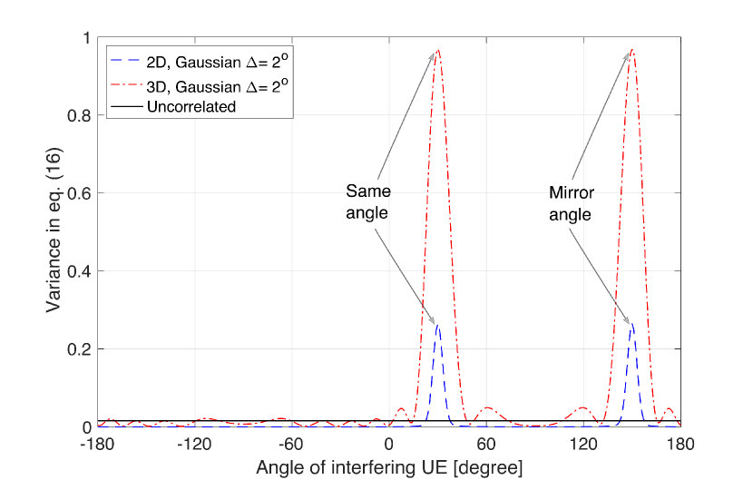
Figure 2: Behaviour of the variance defined in (16) for the same setup of Fig. 1. Uncorrelated fading is also reported for comparison with the 2D and 3D channel models.

To better understand these results, Fig. 2 plots the variance

$$\begin{split}\mathbb{V}\left\{\frac{(\mathbf{h}_{11}^{1})^{\mbox{\tiny$\mathrm{H}$}}\mathbf{h}_{12}^{1}}{\sqrt{\mathbb{E}\{\|\mathbf{h}_{11}^{1}\|^{2}\}\mathbb{E}\{\|\mathbf{h}_{12}^{1}\|^{2}\}}}\right\}=\frac{\mathrm{tr}\left(\mathbf{R}_{11}^{1}\mathbf{R}_{12}^{1}\right)}{\mathrm{tr}(\mathbf{R}_{11}^{1})\mathrm{tr}(\mathbf{R}_{12}^{1})}\end{split}$$ (16)

of the two UEs for 2D and 3D models in the setup of Fig. 1, which measures the so-called favorable propagation condition [1, Eq. (2.19)]. This is a measure of how much interference the two UEs cause to each other. A smaller variance corresponds to lower interference. As seen, it is a function of the spatial correlation matrices of the UEs. Ideally, the variance should be zero. Fig. 1 shows that (16) achieves its maximum values at $30^{\circ}$ and $150^{\circ}$ for both channel models. These correspond to the SE drops in Fig. 1. With the 2D model, the variance peaks are relatively small ($\approx 0.25$), leading to comparatively good favorable propagation conditions. This justifies why classical mMIMO performs well in the setup of Fig. 1(a). On the other hand, the variance is substantially larger ($\approx 0.95$) with the 3D model. This is because the array has only a horizontal spatial resolution given by 8 antennas and a vertical spatial resolution given by 8 antennas, thus it cannot separate the users in any of these domains. Hence, the two UEs cause much interference to each other, and thus the SE of mMIMO deteriorates, especially with MR. This issue can be solved by using NOMA, as shown previously in Fig. 1(b).

IV-B A multi-cell scenario with clusterized UEs

We now extend the SE analysis to a more general scenario with $L=4$ cells. Each BS is equipped with $M=64$ antennas and serve $K$ UEs that are gathered together in a cluster of radius $r$. Each cluster is randomly dropped within its own cell. As for the previous scenario, this setup is quite challenging for conventional mMIMO since the spatial resolution is often insufficient to separate the users, which may result in poor favorable propagation conditions between the UEs. We stress that there are important use cases where this scenario may occur, for example, in stadiums, train stations, public events, and so forth. With NOMA, each cluster is divided into $K/N$ (which is assumed to be an integer) subclusters, each with $N$ UEs. We assume that $N$ orthogonal codes are randomly assigned to the $N$ UEs that belong to a given subcluster.

\begin{overpic}[unit=1mm,width=433.62pt]{SE_funcOfK_random_2D} \end{overpic}

(a) 2D model.

\begin{overpic}[unit=1mm,width=433.62pt]{SE_funcOfK_random_3D} \end{overpic}

(b) 3D model.

Figure 3: Average sum SE for the multi-cell $K$-users setup with $\Delta=2^{\circ}$ vs. $K$ with mMIMO and mMIMO-NOMA for $N\in\{2,4,8\}$. The 2D and 3D models are both considered.

Figure  3 shows the average sum SE per cell as a function of $K$ for mMIMO and mMIMO-NOMA with $N\in\{2,4,8\}$. M-MMSE and MR are considered with both 2D and 3D channel models, and with the angular spread $\Delta=2^{\circ}$. The cluster radius is $r=10$ m and each cluster is randomly positioned at a distance larger than $25$ m from its serving BS. From Fig. 3, we see that the SE of M-MMSE with mMIMO-NOMA achieves better performance than with mMIMO, provided that a good combination of $K$ and $N$ is considered. For example, a $25\%$ gain for 2D model and $35\%$ gain for 3D model are achieved with $N=4$ and $K=32$. This is because the 3D model has a lower resolution in the horizontal/vertical angular domains, which penalizes mMIMO—as also observed in previous work (c.f. [1, Sec. 7.4]). Comparing the results of Figs. 3(a) and 3(b) we observe that the SE of MR is very marginally affected by $N$ in the 2D case, while it increases with $N$ in the 3D case. This is consistent with the basic setup of Sec. IV.A, where the interference between the UEs in the 3D scenario can be reduced by using NOMA. In summary, the above results show that NOMA allows to improve the SE of mMIMO in the considered cases. This happens even if the use of spreading sequences for uplink data transmission introduces an $N$ times lower pre-log factor in the SE expression in (9).

V Conclusions

This paper investigated the potential benefits of code-domain NOMA in Massive MIMO systems. Particularly, we showed that the SE can be improved by using NOMA when poor favorable propagation conditions are experienced by the UEs. This may happen when they are located close to each other and the antenna array does not provide sufficient resolution in the spatial domain. For example, numerical results were used to show that planar rectangular arrays with $M=64$ antennas can benefit from NOMA when the UEs experience poor favorable propagation conditions. This is the type of arrays that are currently being deployed in 4G and 5G networks. These results were obtained both for the heuristic MR combiner and the optimal M-MMSE combiner. This shows that NOMA may help even if schemes with high interference rejection capabilities are employed.

References

- [1] E. Björnson, J. Hoydis, and L. Sanguinetti, “Massive MIMO networks: Spectral, energy, and hardware efficiency,” Foundations and Trends® in Signal Processing, vol. 11, no. 3-4, pp. 154–655, 2017. [Online]. Available: http://dx.doi.org/10.1561/2000000093
- [2] L. Dai, B. Wang, Z. Ding, Z. Wang, S. Chen, and L. Hanzo, “A survey of non-orthogonal multiple access for 5G,” IEEE Communications Surveys Tutorials, vol. 20, no. 3, pp. 2294–2323, thirdquarter 2018.
- [3] M. T. P. Le, G. C. Ferrante, T. Q. S. Quek, and M. Di Benedetto, “Fundamental limits of low-density spreading NOMA with fading,” IEEE Transactions on Wireless Communications, vol. 17, no. 7, pp. 4648–4659, July 2018.
- [4] S. Parkvall, E. Dahlman, A. Furuskär, and M. Frenne, “NR: The new 5G radio access technology,” IEEE Communications Standards Magazine, vol. 1, no. 4, pp. 24–30, Dec 2017.
- [5] K. Senel, H. V. Cheng, E. Björnson, and E. G. Larsson, “What role can NOMA play in massive MIMO?” IEEE Journal of Selected Topics in Signal Processing, vol. 13, no. 3, pp. 597–611, June 2019.
- [6] D. Kudathanthirige and G. A. A. Baduge, “NOMA-aided multicell downlink massive MIMO,” IEEE Journal of Selected Topics in Signal Processing, vol. 13, no. 3, pp. 612–627, June 2019.
- [7] L. Liu, C. Yuen, Y. L. Guan, Y. Li, and C. Huang, “Gaussian message passing for overloaded massive MIMO-NOMA,” IEEE Transactions on Wireless Communications, vol. 18, no. 1, pp. 210–226, Jan 2019.
- [8] M. T. P. Le, G. C. Ferrante, G. Caso, L. De Nardis, and M. Di Benedetto, “On information-theoretic limits of code-domain NOMA for 5G,” IET Communications, vol. 12, no. 15, pp. 1864–1871, 2018.
- [9] D. Zhang, Z. Zhou, C. Xu, Y. Zhang, J. Rodriguez, and T. Sato, “Capacity analysis of NOMA with mmWave massive MIMO systems,” IEEE Journal on Selected Areas in Communications, vol. 35, no. 7, pp. 1606–1618, July 2017.
- [10] J. Ma, C. Liang, C. Xu, and L. Ping, “On orthogonal and superimposed pilot schemes in massive MIMO NOMA systems,” IEEE J. Sel. Areas Commun., vol. 35, no. 12, pp. 2696–2707, Dec 2017.
- [11] E. Björnson, J. Hoydis, and L. Sanguinetti, “Massive MIMO has unlimited capacity,” IEEE Trans. Wireless Commun., vol. 17, no. 1, pp. 574–590, Jan. 2018.
- [12] L. Sanguinetti, E. Björnson, and J. Hoydis, “Towards Massive MIMO 2.0: Understanding spatial correlation, interference suppression, and pilot contamination,” CoRR, vol. abs/1904.03406, 2019. [Online]. Available: https://arxiv.org/abs/1904.03406