Lattice paths and branched continued fractions
II. Multivariate Lah polynomials
and Lah symmetric functions

Abstract

We introduce the generic Lah polynomials $L_{n,k}(\bm{\phi})$, which enumerate unordered forests of increasing ordered trees with a weight $\phi_{i}$ for each vertex with $i$ children. We show that, if the weight sequence $\bm{\phi}$ is Toeplitz-totally positive, then the triangular array of generic Lah polynomials is totally positive and the sequence of row-generating polynomials $L_{n}(\bm{\phi},y)$ is coefficientwise Hankel-totally positive. Upon specialization we obtain results for the Lah symmetric functions and multivariate Lah polynomials of positive and negative type. The multivariate Lah polynomials of positive type are also given by a branched continued fraction. Our proofs use mainly the method of production matrices; the production matrix is obtained by a bijection from ordered forests of increasing ordered trees to labeled partial Łukasiewicz paths. We also give a second proof of the continued fraction using the Euler–Gauss recurrence method.

Key Words: Lah polynomial, Bell polynomial, Eulerian polynomial, symmetric function, increasing tree, forest, Łukasiewicz path, Stirling permutation, continued fraction, branched continued fraction, production matrix, Toeplitz matrix, Hankel matrix, total positivity, Toeplitz-total positivity, Hankel-total positivity.

Mathematics Subject Classification (MSC 2010) codes: 05A15 (Primary); 05A05, 05A18, 05A19, 05A20, 05C30, 05E05, 11B37, 11B73, 15B48, 30B70 (Secondary).

1 Introduction and statement of main results

In a seminal 1980 paper, Flajolet [16] showed that the coefficients in the Taylor expansion of the generic Stieltjes-type (resp. Jacobi-type) continued fraction — which he called the Stieltjes–Rogers (resp. Jacobi–Rogers) polynomials — can be interpreted as the generating polynomials for Dyck (resp. Motzkin) paths with specified height-dependent weights. Very recently it was independently discovered by several authors [17, 34, 26, 42] that Thron-type continued fractions also have an interpretation of this kind: namely, their Taylor coefficients — which we call, by analogy, the Thron–Rogers polynomials — can be interpreted as the generating polynomials for Schröder paths with specified height-dependent weights.

In a recent paper [37] we presented an infinite sequence of generalizations of the Stieltjes–Rogers and Thron–Rogers polynomials, which are parametrized by an integer $m\geq 1$ and reduce to the classical Stieltjes–Rogers and Thron–Rogers polynomials when $m=1$; they are the generating polynomials of $m$-Dyck and $m$-Schröder paths, respectively, with height-dependent weights, and are also the Taylor coefficients of certain branched continued fractions. We proved that these generalizations all possess the fundamental property of coefficientwise Hankel-total positivity [41, 42], jointly in all the (infinitely many) indeterminates. These facts were known when $m=1$ [41, 42] but were new when $m>1$. By specializing the indeterminates we were able to give many examples of Hankel-totally positive sequences whose generating functions do not possess nice classical continued fractions. (The concept of Hankel-total positivity [41, 42] will be explained in more detail later in this Introduction.)

In particular, in [37, section 12] we introduced the multivariate Eulerian polynomials and Eulerian symmetric functions: these are generating polynomials for increasing trees and forests of various types (see below for precise definitions), which vastly extend the classical univariate Eulerian and $r$th-order Eulerian polynomials; we proved their coefficientwise Hankel-total positivity. Here we would like to refine this analysis by considering (among other things) the row-generating polynomials: this leads to defining multivariate Lah polynomials and Lah symmetric functions, which extend the classical univariate Lah polynomials. So let us begin by reviewing briefly some well-known univariate combinatorial polynomials; then we define our multivariate and symmetric-function extensions.

Recall first that the Bell number $B_{n}$ is the number of partitions of an $n$-element set into nonempty blocks; by convention $B_{0}=1$. Refining this, the Stirling subset number (also called Stirling number of the second kind) $\genfrac{\{}{\}}{0.0pt}{}{n}{k}$ is the number of partitions of an $n$-element set into $k$ nonempty blocks; by convention $\genfrac{\{}{\}}{0.0pt}{}{0}{k}=\delta_{k0}$. The Bell polynomials $B_{n}(x)$ are then defined as $B_{n}(x)=\sum_{k=0}^{n}\genfrac{\{}{\}}{0.0pt}{}{n}{k}x^{k}$.

Similarly, the Lah number $L_{n}$ is the number of partitions of an $n$-element set into nonempty linearly ordered blocks (also called lists); we set $L_{0}=1$. Refining this, the Lah number $L(n,k)$ is the number of partitions of an $n$-element set into $k$ nonempty linearly ordered blocks; we set $L(0,k)=\delta_{k0}$. The Lah numbers also have the explicit expression

$$L(n,k)\;=\;{n!\over k!}\binom{n-1}{n-k}\;=\;\begin{cases}\delta_{k0}&\textrm{if $n=0$}\\[5.69054pt] {n!\over k!}\binom{n-1}{k-1}&\textrm{if $n\geq 1$}\end{cases}$$ (1.1)

The Lah polynomials $L_{n}(x)$ are then defined as $L_{n}(x)=\sum_{k=0}^{n}L(n,k)\>x^{k}$.

More generally, let $x$ and ${\mathbf{w}}=\{w_{m}\}_{m\geq 1}$ be indeterminates, and let $P_{n}(x,{\mathbf{w}})$ be the generating polynomial for partitions of an $n$-element set into nonempty blocks in which each block of cardinality $m$ gets a weight $xw_{m}$:

$$P_{n}(x,{\mathbf{w}})\;\stackrel{{\scriptstyle\rm def}}{{=}}\;\sum_{\pi\in\Pi_{n}}x^{|\pi|}\prod_{B\in\pi}w_{|B|}\;.$$ (1.2)

(In particular, the empty set has a unique partition into nonempty blocks — namely, the partition with zero blocks — so that $P_{0}(x,{\mathbf{w}})=1$.) Then the Bell polynomials correspond to $w_{m}=1$, while the Lah polynomials correspond to $w_{m}=m!$. It is not difficult to show that the polynomials $P_{n}(x,{\mathbf{w}})$ have the exponential generating function

$$\sum_{n=0}^{\infty}P_{n}(x,{\mathbf{w}})\,{t^{n}\over n!}\;=\;\exp\biggl{(}x\sum_{m=1}^{\infty}w_{m}\,{t^{m}\over m!}\biggr{)}\;.$$ (1.3)

The polynomials $P_{n}(x,{\mathbf{w}})$ are also known [11, pp. 133–134] as the complete Bell polynomials ${\bf Y}_{n}(xw_{1},\ldots,xw_{n})$.

Let us now express the Bell and Lah polynomials in terms of a different combinatorial object, namely, unordered forests of increasing ordered trees. Recall first [43, pp. 294–295] that an ordered tree (also called plane tree) is a rooted tree in which the children of each vertex are linearly ordered. An unordered forest of ordered trees is an unordered collection of ordered trees. An increasing ordered tree is an ordered tree in which the vertices carry distinct labels from a linearly ordered set (usually some set of integers) in such a way that the label of each child is greater than the label of its parent; otherwise put, the labels increase along every path downwards from the root. An unordered forest of increasing ordered trees is an unordered forest of ordered trees with the same type of labeling.

Now let ${\bm{\phi}}=(\phi_{i})_{i\geq 0}$ be indeterminates, and let $L_{n,k}({\bm{\phi}})$ be the generating polynomial for unordered forests of increasing ordered trees on the vertex set $[n]$, having $k$ components (i.e. $k$ trees), in which each vertex with $i$ children gets a weight $\phi_{i}$. Clearly $L_{n,k}({\bm{\phi}})$ is a homogeneous polynomial of degree $n$ with nonnegative integer coefficients; it is also quasi-homogeneous of degree $n-k$ when $\phi_{i}$ is assigned weight $i$. The first few polynomials $L_{n,k}({\bm{\phi}})$ [specialized for simplicity to $\phi_{0}=1$] are

$n\setminus k$	0	1	2	3	4	5
0	1
1	0	1
2	0	$\phi_{1}$	1
3	0	$\phi_{1}^{2}+2\phi_{2}$	$3\phi_{1}$	1
4	0	$\phi_{1}^{3}+8\phi_{1}\phi_{2}+6\phi_{3}$	$7\phi_{1}^{2}+8\phi_{2}$	$6\phi_{1}$	1
5	0	$\phi_{1}^{4}+22\phi_{1}^{2}\phi_{2}+16\phi_{2}^{2}+42\phi_{1}\phi_{3}+24\phi_{4}$	$15\phi_{1}^{3}+60\phi_{1}\phi_{2}+30\phi_{3}$	$25\phi_{1}^{2}+20\phi_{2}$	$10\phi_{1}$	1

(see also the Appendix for $n\leq 7$). Now let $y$ be an additional indeterminate, and define the row-generating polynomials $L_{n}({\bm{\phi}},y)=\sum_{k=0}^{n}L_{n,k}({\bm{\phi}})\>y^{k}$. Then $L_{n}({\bm{\phi}},y)$ is quasi-homogeneous of degree $n$ when $\phi_{i}$ is assigned weight $i$ and $y$ is assigned weight 1. We call $L_{n,k}({\bm{\phi}})$ and $L_{n}({\bm{\phi}},y)$ the generic Lah polynomials, and we call the lower-triangular matrix ${\sf L}=(L_{n,k}({\bm{\phi}}))_{n,k\geq 0}$ the generic Lah triangle. Here ${\bm{\phi}}=(\phi_{i})_{i\geq 0}$ are in the first instance indeterminates, so that $L_{n,k}({\bm{\phi}})\in{\mathbb{Z}}[{\bm{\phi}}]$ and $L_{n}({\bm{\phi}},y)\in{\mathbb{Z}}[{\bm{\phi}},y]$; but we can then, if we wish, substitute specific values for ${\bm{\phi}}$ in any commutative ring $R$, leading to values $L_{n,k}({\bm{\phi}})\in R$ and $L_{n}({\bm{\phi}},y)\in R[y]$. When doing this we use the same notation $L_{n,k}({\bm{\phi}})$ and $L_{n}({\bm{\phi}},y)$, as the desired interpretation for ${\bm{\phi}}$ should be clear from the context.

Note, finally, that an unordered forest of increasing ordered trees on the vertex set $[n]$, with $k$ components, can be obtained by first choosing a partition of $[n]$ into $k$ nonempty blocks, and then constructing an increasing ordered tree on each block. It follows that the generic Lah polynomial $L_{n}({\bm{\phi}},y)$ equals the set-partition polynomial $P_{n}(y,{\mathbf{w}})$ evaluated at $w_{m}=L_{m,1}({\bm{\phi}})$.

Now let $X=(x_{i})_{i\geq 1}$ be indeterminates, and let ${\bm{e}}=(e_{n}(X))_{n\geq 0}$ and ${\bm{h}}=(h_{n}(X))_{n\geq 0}$ be the elementary symmetric functions and complete homogeneous symmetric functions, respectively; they are elements of the ring ${\mathbb{Z}}[[X]]_{\rm sym}$ of symmetric functions, considered as a subring of the formal-power-series ring ${\mathbb{Z}}[[X]]$. We then define the Lah symmetric functions of positive type by $L_{n,k}^{(\infty)+}(X)=L_{n,k}({\bm{e}})$ and $L_{n}^{(\infty)+}(X,y)=L_{n}({\bm{e}},y)$, and the Lah symmetric functions of negative type by $L_{n,k}^{(\infty)-}(X)=L_{n,k}({\bm{h}})$ and $L_{n}^{(\infty)-}(X,y)=L_{n}({\bm{h}},y)$. Also, for any integer $r\geq 1$ we can imagine specializing $X$ by setting $x_{i}=0$ for $i>r$; we then define the multivariate Lah polynomials of positive type by $L_{n,k}^{(r)+}(x_{1},\ldots,x_{r})=L_{n,k}({\bm{e}}(x_{1},\ldots,x_{r}))$ and $L_{n}^{(r)+}(x_{1},\ldots,x_{r};y)=L_{n}({\bm{e}}(x_{1},\ldots,x_{r}),y)$, and the multivariate Lah polynomials of negative type by $L_{n,k}^{(r)-}(x_{1},\ldots,x_{r})=L_{n,k}({\bm{h}}(x_{1},\ldots,x_{r}))$ and $L_{n}^{(r)-}(x_{1},\ldots,x_{r};y)=L_{n}({\bm{h}}(x_{1},\ldots,x_{r}),y)$. In the Appendix we report the Lah symmetric functions $L_{n,k}^{(\infty)+}$ and $L_{n,k}^{(\infty)-}$ for $n\leq 7$ in terms of the monomial symmetric functions $m_{\lambda}$.

These multivariate Lah polynomials and symmetric functions can also be interpreted as generating polynomials for increasing $r$-ary and multi-$r$-ary trees and forests ($1\leq r\leq\infty$). Let us recall first [43, p. 295] the recursive definition of an $r$-ary tree ($1\leq r<\infty$): it is either empty or else consists of a root together with an ordered list of $r$ subtrees, each of which is an $r$-ary tree (which may be empty). We draw an edge from each vertex to the root of each of its nonempty subtrees; an edge from a vertex to the root of its $i$th subtree will be called an $i$-edge. Similarly, we can define recursively an $\infty$-ary tree: it is either empty or else consists of a root together with an ordered list of subtrees indexed by the positive integers ${\mathbb{P}}$, each of which is an $\infty$-ary tree (which may be empty) and only finitely many of which are nonempty; we define $i$-edges as before. But we can now view $r$-ary trees from a slightly different point of view: an $r$-ary (resp. $\infty$-ary) tree is simply an ordered tree in which each edge carries a label $i\in[r]$ (resp. $i\in{\mathbb{P}}$) and the edges emanating outwards from each vertex consist, in order, of zero or one edges labeled 1, then zero or one edges labeled 2, and so forth; an edge with label $i$ will be called an $i$-edge. Let us now consider the generating polynomial for unordered forests of increasing $\infty$-ary trees on the vertex set $[n]$, having $k$ components, in which each $i$-edge gets a weight $x_{i}$. Since the choice of labels on the edges emanating outwards from a vertex $v$ can be made independently for each $v$, this is equivalent to evaluating the generating polynomial $L_{n,k}({\bm{\phi}})$ at $\phi_{i}=e_{i}(X)$; in other words, it is the Lah symmetric function of positive type $L_{n,k}^{(\infty)+}(X)=L_{n,k}({\bm{e}})$. Similarly, $L_{n}^{(\infty)+}(X,y)=L_{n}({\bm{e}},y)$ is the generating polynomial for unordered forests of increasing $\infty$-ary trees on the vertex set $[n]$, in which each $i$-edge gets a weight $x_{i}$ and each tree (or equivalently, each root) gets a weight $y$. And if we set $x_{i}=0$ for $i>r$ so as to obtain $r$-ary trees or forests, we get the multivariate Lah polynomials $L_{n,k}^{(r)+}(x_{1},\ldots,x_{r})=L_{n,k}({\bm{e}}(x_{1},\ldots,x_{r}))$ and $L_{n}^{(r)+}(x_{1},\ldots,x_{r};y)=L_{n}({\bm{e}}(x_{1},\ldots,x_{r}),y)$.

The multivariate Lah polynomials and Lah symmetric functions of negative type can be interpreted in a similar way. We begin by adopting the reinterpretation of $r$-ary and $\infty$-ary trees as ordered trees with labeled edges, and then consider [37, section 10.3.2] the variant in which the number of edges of each label emanating from a given vertex, instead of being “zero or one”, is “zero or more”: we call this a multi-$r$-ary (resp. multi-$\infty$-ary) tree. We now consider the generating polynomial for unordered forests of increasing multi-$\infty$-ary trees on the vertex set $[n]$, having $k$ components, in which each $i$-edge gets a weight $x_{i}$. This is equivalent to evaluating the generating polynomial $L_{n,k}({\bm{\phi}})$ at $\phi_{i}=h_{i}(X)$; in other words, it is the Lah symmetric function of negative type $L_{n,k}^{(\infty)-}(X)=L_{n,k}({\bm{h}})$. Similarly, $L_{n}^{(\infty)-}(X,y)=L_{n}({\bm{h}},y)$ is the generating polynomial for unordered forests of increasing multi-$\infty$-ary trees on the vertex set $[n]$, in which each $i$-edge gets a weight $x_{i}$ and each tree (or equivalently, each root) gets a weight $y$. And if we set $x_{i}=0$ for $i>r$ so as to obtain multi-$r$-ary trees or forests, we get the multivariate Lah polynomials $L_{n,k}^{(r)-}(x_{1},\ldots,x_{r})=L_{n,k}({\bm{h}}(x_{1},\ldots,x_{r}))$ and $L_{n}^{(r)-}(x_{1},\ldots,x_{r};y)=L_{n}({\bm{h}}(x_{1},\ldots,x_{r}),y)$.

Let us now consider the further specialization of the multivariate Lah polynomials of positive type to $x_{1}=\ldots=x_{r}=1$, corresponding to $\phi_{i}=\binom{r}{i}$. It is well known [43, p. 24] that the number of increasing binary trees on $n$ vertices is $n!$, and more generally that the number of increasing $r$-ary trees on $n$ vertices is the multifactorial $F_{n}^{(r-1)}$ [4, p. 30, Example 1], where

$$F_{n}^{(r)}\;\stackrel{{\scriptstyle\rm def}}{{=}}\;\prod_{j=0}^{n-1}(1+jr)\;.$$ (1.4)

Therefore, the univariate $r$th-order Lah polynomials of positive type, $L_{n}^{(r)+}({\bm{1}};y)$, coincide with the set-partition polynomials $P_{n}(y,{\mathbf{w}})$ defined in (1.2) when we set $w_{m}=F_{m}^{(r-1)}$. In particular, for $r=1$ we have $w_{m}=1$ and obtain the Bell polynomials $B_{n}(y)$; for $r=2$ we have $w_{m}=m!$ and obtain the univariate Lah polynomials $L_{n}(y)$; for $r=3,4,5$ we have $w_{m}=(2m-1)!!,(3m-2)!!!,(4m-3)!!!!$ and obtain the row-generating polynomials of [33, A035342, A035469, A049029].

In a similar way, we can specialize the multivariate Lah polynomials of negative type to $x_{1}=\ldots=x_{r}=1$, corresponding to $\phi_{i}=\binom{r+i-1}{i}$. It is known [4, p. 30, Corollary 1(iv)] that the number of increasing multi-unary trees on $n$ vertices is $(2n-3)!!$; more generally, it was observed in [37, section 12.3] that the number of increasing multi-$r$-ary trees on $n$ vertices is the shifted multifactorial $\widetilde{F}_{n-1}^{(r+1)}$, where

$$\widetilde{F}_{n}^{(r)}\;\stackrel{{\scriptstyle\rm def}}{{=}}\;\prod\limits_{j=0}^{n-1}[(r-1)+jr]\;.$$ (1.5)

Therefore, the univariate $r$th-order Lah polynomials of negative type, $L_{n}^{(r)-}({\bm{1}};y)$, coincide with the set-partition polynomials $P_{n}(y,{\mathbf{w}})$ defined in (1.2) when we set $w_{m}=\widetilde{F}_{m-1}^{(r+1)}$. In particular, for $r=1$ we have $w_{m}=(2m-3)!!$ and obtain a variant of the Bessel polynomials [33, A001497] (see also Example 7.1 below); for $r=2,3$ we have $w_{m}=(3m-4)!!!,(4m-5)!!!!$ and obtain the row-generating polynomials of [33, A004747, A000369].

Let us now explain how all this relates to total positivity. Recall first that a finite or infinite matrix of real numbers is called totally positive (TP) if all its minors are nonnegative, and totally positive of order $r$ (TP_r) if all its minors of size $\leq r$ are nonnegative. Background information on totally positive matrices can be found in [27, 18, 38, 15]; they have application to many fields of pure and applied mathematics. In particular, it is known [19, Théorème 9] [38, section 4.6] that a Hankel matrix $(a_{i+j})_{i,j\geq 0}$ of real numbers is totally positive if and only if the underlying sequence $(a_{n})_{n\geq 0}$ is a Stieltjes moment sequence (i.e. the moments of a positive measure on $[0,\infty)$). And a Toeplitz matrix $(a_{i-j})_{i,j\geq 0}$ of real numbers (where $a_{n}=0$ for $n<0$) is totally positive if and only if its ordinary generating function can be written as

$$\sum_{n=0}^{\infty}a_{n}t^{n}\;=\;Ce^{\gamma t}t^{m}\prod_{i=1}^{\infty}{1+\alpha_{i}t\over 1-\beta_{i}t}$$ (1.6)

with $m\in{\mathbb{N}}$, $C,\gamma,\alpha_{i},\beta_{i}\geq 0$, $\sum\alpha_{i}<\infty$ and $\sum\beta_{i}<\infty$ [27, Theorem 5.3, p. 412].

But this is only the beginning of the story, because we are here principally concerned, not with sequences and matrices of real numbers, but with sequences and matrices of polynomials (with integer or real coefficients) in one or more indeterminates ${\mathbf{x}}$: they will typically be generating polynomials that enumerate some combinatorial objects with respect to one or more statistics. We equip the polynomial ring ${\mathbb{R}}[{\mathbf{x}}]$ with the coefficientwise partial order: that is, we say that $P$ is nonnegative (and write $P\succeq 0$) in case $P$ is a polynomial with nonnegative coefficients. We then say that a matrix with entries in ${\mathbb{R}}[{\mathbf{x}}]$ is coefficientwise totally positive if all its minors are polynomials with nonnegative coefficients; and analogously for coefficientwise total positivity of order $r$. We say that a sequence ${\bm{a}}=(a_{n})_{n\geq 0}$ with entries in ${\mathbb{R}}[{\mathbf{x}}]$ is coefficientwise Hankel-totally positive (resp. coefficientwise Toeplitz-totally positive) if its associated infinite Hankel (resp. Toeplitz) matrix is coefficientwise totally positive; and likewise for the versions of order $r$. Similar definitions apply to the formal-power-series ring ${\mathbb{R}}[[{\mathbf{x}}]]$. Most generally, we can consider sequences and matrices with values in an arbitrary partially ordered commutative ring (a precise definition will be given in Section 2.1); total positivity, Hankel-total positivity and Toeplitz-total positivity are then defined in the obvious way.

Let us also explain some partial orders on the ring of symmetric functions. Let $R$ be a commutative ring and let ${\mathbf{X}}=(x_{i})_{i\geq 1}$ be a countably infinite collection of indeterminates. Then let $R[[{\mathbf{X}}]]_{\rm sym}$ be the ring of symmetric functions with coefficients in $R$ [31, Chapter 1] [44, Chapter 7]; it is a subring of the formal-power-series ring $R[[{\mathbf{X}}]]$. (It goes without saying that “function” is a misnomer; these are formal power series.) Now let $R$ carry a partial order ${\mathcal{P}}$. When the coefficientwise order on $R[[{\mathbf{X}}]]$ is restricted to $R[[{\mathbf{X}}]]_{\rm sym}$, it becomes the monomial order: an element $f\in R[[{\mathbf{X}}]]_{\rm sym}$ is monomial-nonnegative if and only if it can be written as a (finite) nonnegative linear combination of monomial symmetric functions $m_{\lambda}({\mathbf{X}})$. However, the ring of symmetric functions can also be equipped with a stronger order, namely the Schur order: an element $f\in R[[{\mathbf{X}}]]_{\rm sym}$ is Schur-nonnegative if and only if it can be written as a (finite) nonnegative linear combination of Schur functions $s_{\lambda}({\mathbf{X}})$. This indeed defines a partial order compatible with the ring structure, since any product of Schur functions is a nonnegative linear combination of Schur functions (Littlewood–Richardson coefficients [44, Section 7.A1.3]). And it is strictly stronger than the monomial order, because every Schur function is a nonnegative linear combination of monomial symmetric functions (Kostka numbers [44, eq. (7.35), p. 311]) but not conversely (e.g. $m_{2}=s_{2}-s_{11}$).

We can now state our main result:

Theorem 1.1 (Total positivity of Lah matrices and Lah polynomials).

Fix $1\leq r\leq\infty$. Let $R$ be a partially ordered commutative ring, and let ${\bm{\phi}}=(\phi_{i})_{i\geq 0}$ be a sequence in $R$ that is Toeplitz-totally positive of order $r$. Then:

• The lower-triangular matrix ${\sf L}({\bm{\phi}})=(L_{n,k}({\bm{\phi}}))_{n,k\geq 0}$ is totally positive of order $r$ in the ring $R$.

• The sequence ${\bm{L}}({\bm{\phi}})=(L_{n}({\bm{\phi}},y))_{n\geq 0}$ is Hankel-totally positive of order $r$ in the ring $R[y]$ equipped with the coefficientwise order.

• The sequence ${\bm{L}}^{\triangle}({\bm{\phi}})=(L_{n+1,1}({\bm{\phi}}))_{n\geq 0}$ is Hankel-totally positive of order $r$ in the ring $R$.

Specializing this to ${\bm{\phi}}={\bm{e}}(X)$ or ${\bm{h}}(X)$ and using the Jacobi–Trudi identity [44, Theorem 7.16.1 and Corollary 7.16.2], we obtain:

Corollary 1.2 (Total positivity of Lah symmetric functions).

• The unit-lower-triangular matrices ${\sf L}^{(\infty)+}=(L_{n,k}({\bm{e}}(X)))_{n,k\geq 0}$ and ${\sf L}^{(\infty)-}=$ $(L_{n,k}({\bm{h}}(X)))_{n,k\geq 0}$ are totally positive with respect to the Schur order on the ring of symmetric functions (with coefficients in ${\mathbb{Z}}$).

• The sequences ${\bm{L}}^{(\infty)+}=(L_{n}({\bm{e}}(X),y))_{n\geq 0}$ and ${\bm{L}}^{(\infty)-}=(L_{n}({\bm{h}}(X),y))_{n\geq 0}$ are Hankel-totally positive with respect to the Schur order on the ring of symmetric functions (with coefficients in ${\mathbb{Z}}$) and the coefficientwise order on polynomials in $y$.

• The sequences ${\bm{L}}^{(\infty)+\triangle}=(L_{n+1,1}({\bm{e}}(X)))_{n\geq 0}$ and ${\bm{L}}^{(\infty)-\triangle}=(L_{n+1,1}({\bm{h}}(X)))_{n\geq 0}$ are Hankel-totally positive with respect to the Schur order on the ring of symmetric functions (with coefficients in ${\mathbb{Z}}$).

Weakening this result from the Schur order to the monomial order, and then further specializing by setting $x_{i}=0$ for $i>r$, we obtain:

Corollary 1.3 (Total positivity of multivariate Lah polynomials).

• The unit-lower-triangular matrices ${\sf L}^{(r)+}=(L_{n,k}({\bm{e}}(x_{1},\ldots,x_{r})))_{n,k\geq 0}$ and ${\sf L}^{(r)-}=(L_{n,k}({\bm{h}}(x_{1},\ldots,x_{r})))_{n,k\geq 0}$ are totally positive with respect to the coefficientwise order on the polynomial ring ${\mathbb{Z}}[x_{1},\ldots,x_{r}]$.

• The sequences ${\bm{L}}^{(r)+}=(L_{n}({\bm{e}}(x_{1},\ldots,x_{r}),y))_{n\geq 0}$ and ${\bm{L}}^{(r)-}=$    $(L_{n}({\bm{h}}(x_{1},\ldots,x_{r}),y))_{n\geq 0}$ are Hankel-totally positive with respect to the coefficientwise order on the polynomial ring ${\mathbb{Z}}[x_{1},\ldots,x_{r},y]$.

• The sequences ${\bm{L}}^{(r)+\triangle}=(L_{n+1,1}({\bm{e}}(x_{1},\ldots,x_{r})))_{n\geq 0}$ and ${\bm{L}}^{(r)-\triangle}=$    $(L_{n+1,1}({\bm{h}}(x_{1},\ldots,x_{r})))_{n\geq 0}$ are Hankel-totally positive with respect to the coefficientwise order on the polynomial ring ${\mathbb{Z}}[x_{1},\ldots,x_{r}]$.

Remarks. 1. In Theorem 1.1 and its two corollaries, part (c) follows trivially from part (b) by dividing $L_{n+1}({\bm{\phi}},y)$ by $y$ and then specializing to $y=0$. But in Section 3 we will introduce a generalization where the analogue of (c) still holds (by a different proof), but it is unknown whether there is any analogue of (b).

2. Corollaries 1.2(a) and 1.3(a) are essentially already contained in [37, Corollaries 12.5 and 12.25 and Remark after the proof of Lemma 12.13]. But the extension in Theorem 1.1(a) to the generic Lah polynomials is new.

3. Similarly, Corollaries 1.2(c) and 1.3(c) are already contained in [37, Corollaries 12.3 and 12.24]. Indeed, a slightly stronger version of Corollaries 1.2(c) and 1.3(c) for ${\sf L}^{(\infty)+}$ and ${\sf L}^{(r)+}$ — in which the Hankel-totally positive sequence is extended backwards by prepending one element — is given in [37, Theorem 12.1(a) and Corollaries 12.3 and 12.7]. There is also an analogous result for the case of negative type [37, Theorem 12.20(a) and Corollary 12.22], but it does not seem to imply (at least in any obvious way) the negative-type case of Corollaries 1.2(c) and 1.3(c). $\blacksquare$

Our proof of Theorem 1.1 will be based on the method of production matrices [12, 13]. We shall review this theory in Sections 2.2 and 2.3, so now we state only the bare-bones definitions. Let $P=(p_{ij})_{i,j\geq 0}$ be an infinite matrix with entries in a commutative ring $R$; we assume that $P$ is either row-finite (i.e. has only finitely many nonzero entries in each row) or column-finite. Now define an infinite matrix $A=(a_{nk})_{n,k\geq 0}$ by

$$a_{nk}\;=\;(P^{n})_{0k}\;.$$ (1.7)

We call $P$ the production matrix and $A$ the output matrix, and we write $A={\mathcal{O}}(P)$. The two key facts here are the following [42]: if $R$ is a partially ordered commutative ring and $P$ is totally positive of order $r$, then ${\mathcal{O}}(P)$ is totally positive of order $r$ and the zeroth column of ${\mathcal{O}}(P)$ is Hankel-totally positive of order $r$. See Section 2.3 for precise statements and proofs.

We shall prove Theorem 1.1 by explicitly constructing the production matrix that generates the the generic Lah triangle ${\sf L}=(L_{n,k}({\bm{\phi}}))_{n,k\geq 0}$, and then verifying its total positivity. Let $\Delta=(\delta_{i+1,j})_{i,j\geq 0}$ be the matrix with 1 on the superdiagonal and 0 elsewhere. We then have:

Proposition 1.4 (Production matrix for the generic Lah triangle).

Let ${\bm{\phi}}=(\phi_{i})_{i\geq 0}$ and $y$ be indeterminates, and work in the ring ${\mathbb{Z}}[{\bm{\phi}},y]$. Define the lower-Hessenberg matrix $P=(p_{ij})_{i,j\geq 0}$ by

$$p_{ij}\;=\;\begin{cases}0&\textrm{if $j=0$ or $j>i+1$}\\[2.84526pt] {\displaystyle{i!\over(j-1)!}}\,\phi_{i-j+1}&\textrm{if $1\leq j\leq i+1$}\end{cases}$$ (1.8)

and the unit-lower-triangular $y$-binomial matrix $B_{y}$ by

$$(B_{y})_{nk}\;=\;\binom{n}{k}\,y^{n-k}\;.$$ (1.9)

Then:

• $P$ is the production matrix for the generic Lah triangle ${\sf L}=(L_{n,k}({\bm{\phi}}))_{n,k\geq 0}$.

• $B_{y}^{-1}PB_{y}=P(I+y\Delta^{\rm T})$ is the production matrix for ${\sf L}B_{y}$.

We will prove Proposition 1.4(a) by constructing a bijection from ordered forests of increasing ordered trees to labeled partial Łukasiewicz paths, along the lines of [37, proofs of Theorems 12.11 and 12.28]. Then Proposition 1.4(b) will follow by a straightforward but slightly nontrivial computation (Lemma 3.6).

In fact, we will prove a generalization of Proposition 1.4(a) [and hence also of Theorem 1.1(a,c) and Corollaries 1.2(a,c) and 1.3(a,c)] for some polynomials ${\widehat{L}}_{n,k}({{\widehat{\vphantom{t}\smash{\bm{\phi}}\mkern 3.0mu}\mkern-3.0mu}{}})$, to be defined in Section 3.1, that depend on a refined set of indeterminates ${{\widehat{\vphantom{t}\smash{\bm{\phi}}\mkern 3.0mu}\mkern-3.0mu}{}}=(\phi_{i}^{[L]})_{i\geq 0,\,L\geq 1}$ and that reduce to $L_{n,k}({\bm{\phi}})$ when $\phi_{i}^{[L]}=\phi_{i}$ for all $L$. However, no analogue of Proposition 1.4(b) [and hence also of Theorem 1.1(b) and Corollaries 1.2(b) and 1.3(b)] appears to exist for these more general polynomials.

Remark. If we were to work in the ring ${\mathbb{Q}}[{\bm{\phi}},y]$ instead of ${\mathbb{Z}}[{\bm{\phi}},y]$, we would have $P=DT_{\infty}({\bm{\phi}})D^{-1}\Delta$ where $T_{\infty}({\bm{\phi}})$ is the infinite lower-triangular Toeplitz matrix associated to the sequence ${\bm{\phi}}$, and $D=\mathop{\rm diag}\nolimits\bigl{(}(n!)_{n\geq 0}\bigr{)}$. $\blacksquare$

Now return to the situation of Theorem 1.1. If the ring $R$ contains the rationals (with their usual order), it follows from $P=DT_{\infty}({\bm{\phi}})D^{-1}\Delta$ that $P$ is totally positive of order $r$ whenever ${\bm{\phi}}$ is Toeplitz-totally positive of order $r$; and the same holds for $B_{y}^{-1}PB_{y}=P(I+y\Delta^{\rm T})$. And even if $R$ does not contain the rationals, it turns out that the same conclusions are true, as we can show with a bit more work (Lemma 3.7). Theorem 1.1 is then an immediate consequence of Proposition 1.4 and Lemma 3.7 together with the general theory of production matrices and total positivity (Section 2.3).

Now fix an integer $r\geq 1$, and let us consider the multivariate Lah polynomials of positive type by specializing the production matrix (1.8) to $\phi_{n}=e_{n}(x_{1},\ldots,x_{r})$. Recall that the product of two lower-triangular Toeplitz matrices corresponds to the convolution of their generating sequences, or equivalently the product of their ordinary generating functions; and since $\sum\limits_{n=0}^{\infty}e_{n}(x_{1},\ldots,x_{r})\,t^{n}=\prod\limits_{i=1}^{r}(1+x_{i}t)$, it follows that the lower-triangular Toeplitz matrix $T_{\infty}({\bm{e}}(x_{1},\ldots,x_{r}))$ has the factorization $T_{\infty}({\bm{e}})=L_{1}\cdots L_{r}$ where $L_{i}=L(1,1,\ldots;x_{i},x_{i},\ldots)$ is the lower-bidiagonal Toeplitz matrix with 1 on the diagonal and $x_{i}$ on the subdiagonal. Therefore, $DT_{\infty}({\bm{e}})D^{-1}$ has the factorization $L^{\prime}_{1}\cdots L^{\prime}_{r}$ where $L^{\prime}_{i}=DL_{i}D^{-1}=L(1,1,\ldots;x_{i},2x_{i},3x_{i},\ldots)$; the production matrix $P(x_{1},\ldots,x_{r})=DT_{\infty}({\bm{e}})D^{-1}\Delta$ has the factorization $L^{\prime}_{1}\cdots L^{\prime}_{r}\Delta$; and the modified production matrix $B_{y}^{-1}PB_{y}=P(I+y\Delta^{\rm T})$ has the factorization

$$B_{y}^{-1}\,P(x_{1},\ldots,x_{r})\,B_{y}\;=\;L^{\prime}_{1}\,\cdots\,L^{\prime}_{r}\,(\Delta+yI)$$ (1.10)

(since $\Delta\Delta^{\rm T}=I$). On the other hand, (1.10) is precisely the production matrix for an $r$-branched S-fraction with coefficients

$${\bm{\alpha}}\;=\;(\alpha_{i})_{i\geq r}\;=\;y,x_{1},\ldots,x_{r},y,2x_{1},\ldots,2x_{r},y,3x_{1},\ldots,3x_{r},\ldots$$ (1.11)

(see [37, Propositions 7.2 and 8.2(b)] and eq. (2.21) below). Since the zeroth column of the matrix ${\sf L}B_{y}$ is given by the Lah polynomials $L_{n}({\bm{\phi}},y)$, it follows that the multivariate Lah polynomials of positive type $L_{n}^{(r)+}(x_{1},\ldots,x_{r};y)$ are given by an $r$-branched S-fraction with coefficients (1.11):

Theorem 1.5 (Branched S-fraction for multivariate Lah polynomials of positive type).

We have $L_{n}^{(r)+}(x_{1},\ldots,x_{r};y)=S_{n}^{(r)}({\bm{\alpha}})$ where the coefficients ${\bm{\alpha}}$ are given by (1.11). [Here $S_{n}^{(r)}({\bm{\alpha}})$ is the $r$-Stieltjes–Rogers polynomial of order $n$; see Section 2.4 for the precise definition.]

Remarks. 1. For $r=1$ the multivariate Lah polynomials of positive type are simply the homogenized Bell polynomials $L_{n}^{(1)+}(x_{1};y)=x_{1}^{n}B_{n}(y/x_{1})$, and this is the well-known classical S-fraction with coefficients ${\bm{\alpha}}=y,x_{1},y,2x_{1},y,3x_{1},\ldots$.

2. Since $L_{n}^{(r)+}(x_{1},\ldots,x_{r};y)$ is invariant under permutations of $x_{1},\ldots,x_{r}$, it is actually represented by $r!$ different $r$-branched S-fractions in which the coefficients ${\bm{\alpha}}$ are obtained from (1.11) by permuting $x_{1},\ldots,x_{r}$. This illustrates the nonuniqueness of $r$-branched S-fractions for $r\geq 2$ [37].

3. In Section 5 we will also give a completely independent proof of Theorem 1.5, based on the Euler–Gauss recurrence method. $\blacksquare$

For the multivariate Lah polynomials of negative type, the lower-triangular Toeplitz matrix $T_{\infty}({\bm{h}}(x_{1},\ldots,x_{r}))$ has the factorization $T_{\infty}({\bm{h}})={\widetilde{L}}_{1}\cdots{\widetilde{L}}_{r}$ where ${\widetilde{L}}_{i}=$ $L(1,1,\ldots;-x_{i},-x_{i},\ldots)^{-1}$; so $DT_{\infty}({\bm{h}})D^{-1}$ has the factorization ${\widetilde{L}}^{\prime}_{1}\cdots{\widetilde{L}}^{\prime}_{r}$ where ${\widetilde{L}}^{\prime}_{i}=D{\widetilde{L}}_{i}D^{-1}=L(1,1,\ldots;-x_{i},-2x_{i},-3x_{i},\ldots)^{-1}$; and the production matrix $DT_{\infty}({\bm{h}})D^{-1}\Delta$ has the factorization ${\widetilde{L}}^{\prime}_{1}\cdots{\widetilde{L}}^{\prime}_{r}\Delta$. But the matrices ${\widetilde{L}}_{i}$ and ${\widetilde{L}}^{\prime}_{i}$ are dense lower-triangular, not lower-bidiagonal, so we do not see any way of interpreting this as the production matrix of a branched S-fraction. Indeed, we have verified that the multivariate Lah numbers of negative type $L_{n}^{(r)-}(1,\ldots,1;1)$ cannot be expressed as an $m$-branched S-fraction of the following types:

• For $r=1,2,3$, the numbers $L_{n}^{(r)-}(1,\ldots,1;1)$ cannot be expressed as a 2-branched S-fraction with nonnegative integer coefficients: this was verified by exhaustive computer search using $n\leq 7,8,7$, respectively.

• For $m>r+1$, the numbers $a_{n}=L_{n}^{(r)-}(1,\ldots,1;1)$ cannot be expressed as an $m$-branched S-fraction with positive integer coefficients: this is simply because $a_{0}=a_{1}=1$ and $a_{2}=r+1$, while the $m$-Stieltjes–Rogers polynomial $S_{2}^{(m)}({\bm{\alpha}})$ equals $\alpha_{m}(\alpha_{m}+\alpha_{m+1}+\cdots+\alpha_{2m-1})$.

For $(r,m)=(1,3)$ and $(2,3)$, our computations (as far as we were able to go) were unable to give either a proof of nonexistence (with nonnegative integer coefficients) or a comprehensible candidate for ${\bm{\alpha}}$.

Although the present paper is a follow-up to our paper [37], we have endeavored, for the convenience of the reader, to make it as self-contained as possible. We have therefore begun (Section 2) with a brief review of the key definitions and results from [37] that will be needed in the sequel. We then proceed as follows: In Section 3 — which is the technical heart of the paper — we prove Proposition 1.4, from which we deduce Theorem 1.1; indeed, we state and prove a generalization involving a refined set of indeterminates. In Section 4 we give expressions for the multivariate Lah polynomials of positive and negative type in terms of the action of certain first-order linear differential operators. In Section 5 we give a second proof of Theorem 1.5, based on the differential operators and the Euler–Gauss recurrence method. In Section 6 we interpret the multivariate Lah polynomials of positive type $L_{n}^{(r)+}({\mathbf{x}},y)$ as generating polynomials for partitions of the set $[n]$ in which each block is “decorated” with an additional structure. In Section 7 we compute explicit expressions for the generic Lah polynomials $L_{n,k}({\bm{\phi}})$ by using exponential generating functions. In the Note Added (Section 8) we give an alternate proof of Proposition 1.4(a), using the theory of exponential Riordan arrays. In the Appendix we report the generic Lah polynomials and Lah symmetric functions for $n\leq 7$.

2 Preliminaries

Here we review some definitions and results from [37] that will be needed in the sequel.

2.1 Partially ordered commutative rings and total positivity

In this paper all rings will be assumed to have an identity element 1 and to be nontrivial ($1\neq 0$).

A partially ordered commutative ring is a pair $(R,{\mathcal{P}})$ where $R$ is a commutative ring and ${\mathcal{P}}$ is a subset of $R$ satisfying

• $0,1\in{\mathcal{P}}$.

• If $a,b\in{\mathcal{P}}$, then $a+b\in{\mathcal{P}}$ and $ab\in{\mathcal{P}}$.

• ${\mathcal{P}}\cap(-{\mathcal{P}})=\{0\}$.

We call ${\mathcal{P}}$ the nonnegative elements of $R$, and we define a partial order on $R$ (compatible with the ring structure) by writing $a\leq b$ as a synonym for $b-a\in{\mathcal{P}}$. Please note that, unlike the practice in real algebraic geometry [6, 29, 39, 32], we do not assume here that squares are nonnegative; indeed, this property fails completely for our prototypical example, the ring of polynomials with the coefficientwise order, since $(1-x)^{2}=1-2x+x^{2}\not\succeq 0$.

Now let $(R,{\mathcal{P}})$ be a partially ordered commutative ring and let ${\mathbf{x}}=\{x_{i}\}_{i\in I}$ be a collection of indeterminates. In the polynomial ring $R[{\mathbf{x}}]$ and the formal-power-series ring $R[[{\mathbf{x}}]]$, let ${\mathcal{P}}[{\mathbf{x}}]$ and ${\mathcal{P}}[[{\mathbf{x}}]]$ be the subsets consisting of polynomials (resp. series) with nonnegative coefficients. Then $(R[{\mathbf{x}}],{\mathcal{P}}[{\mathbf{x}}])$ and $(R[[{\mathbf{x}}]],{\mathcal{P}}[[{\mathbf{x}}]])$ are partially ordered commutative rings; we refer to this as the coefficientwise order on $R[{\mathbf{x}}]$ and $R[[{\mathbf{x}}]]$.

A (finite or infinite) matrix with entries in a partially ordered commutative ring is called totally positive (TP) if all its minors are nonnegative; it is called totally positive of order $\bm{r}$ (TP_r) if all its minors of size $\leq r$ are nonnegative. It follows immediately from the Cauchy–Binet formula that the product of two TP (resp. TP_r) matrices is TP (resp. TP_r). This fact is so fundamental to the theory of total positivity that we shall henceforth use it without comment.

We say that a sequence ${\bm{a}}=(a_{n})_{n\geq 0}$ with entries in a partially ordered commutative ring is Hankel-totally positive (resp. Hankel-totally positive of order $\bm{r}$) if its associated infinite Hankel matrix $H_{\infty}({\bm{a}})=(a_{i+j})_{i,j\geq 0}$ is TP (resp. TP_r). We say that ${\bm{a}}$ is Toeplitz-totally positive (resp. Toeplitz-totally positive of order $\bm{r}$) if its associated infinite Toeplitz matrix $T_{\infty}({\bm{a}})=(a_{i-j})_{i,j\geq 0}$ (where $a_{n}\stackrel{{\scriptstyle\rm def}}{{=}}0$ for $n<0$) is TP (resp. TP_r).

We will need an easy fact about the total positivity of special matrices:

Lemma 2.1 (Bidiagonal matrices).

Let $A$ be a matrix with entries in a partially ordered commutative ring, with the property that all its nonzero entries belong to two consecutive diagonals. Then $A$ is totally positive if and only if all its entries are nonnegative.

Proof. The nonnegativity of the entries (i.e. TP₁) is obviously a necessary condition for TP. Conversely, for a matrix of this type it is easy to see that every nonzero minor is simply a product of some entries. $\square$

2.2 Production matrices

The method of production matrices [12, 13] has become in recent years an important tool in enumerative combinatorics. In the special case of a tridiagonal production matrix, this construction goes back to Stieltjes’ [45, 46] work on continued fractions: the production matrix of a classical S-fraction or J-fraction is tridiagonal. In the present paper, by contrast, we shall need production matrices that are lower-Hessenberg (i.e. vanish above the first superdiagonal) but are not in general tridiagonal. We therefore begin by reviewing briefly the basic theory of production matrices. The important connection of production matrices with total positivity will be treated in the next subsection.

Let $P=(p_{ij})_{i,j\geq 0}$ be an infinite matrix with entries in a commutative ring $R$. In order that powers of $P$ be well-defined, we shall assume that $P$ is either row-finite (i.e. has only finitely many nonzero entries in each row) or column-finite.

Let us now define an infinite matrix $A=(a_{nk})_{n,k\geq 0}$ by

$$a_{nk}\;=\;(P^{n})_{0k}$$ (2.1)

(in particular, $a_{0k}=\delta_{0k}$). Writing out the matrix multiplications explicitly, we have

$$a_{nk}\;=\;\sum_{i_{1},\ldots,i_{n-1}}p_{0i_{1}}\,p_{i_{1}i_{2}}\,p_{i_{2}i_{3}}\,\cdots\,p_{i_{n-2}i_{n-1}}\,p_{i_{n-1}k}\;,$$ (2.2)

so that $a_{nk}$ is the total weight for all $n$-step walks in ${\mathbb{N}}$ from $i_{0}=0$ to $i_{n}=k$, in which the weight of a walk is the product of the weights of its steps, and a step from $i$ to $j$ gets a weight $p_{ij}$. Yet another equivalent formulation is to define the entries $a_{nk}$ by the recurrence

$$a_{nk}\;=\;\sum_{i=0}^{\infty}a_{n-1,i}\,p_{ik}\qquad\hbox{for $n\geq 1$}$$ (2.3)

with the initial condition $a_{0k}=\delta_{0k}$.

We call $P$ the production matrix and $A$ the output matrix, and we write $A={\mathcal{O}}(P)$. Note that if $P$ is row-finite, then so is ${\mathcal{O}}(P)$; if $P$ is lower-Hessenberg, then ${\mathcal{O}}(P)$ is lower-triangular; if $P$ is lower-Hessenberg with invertible superdiagonal entries, then ${\mathcal{O}}(P)$ is lower-triangular with invertible diagonal entries; and if $P$ is unit-lower-Hessenberg (i.e. lower-Hessenberg with entries 1 on the superdiagonal), then ${\mathcal{O}}(P)$ is unit-lower-triangular. In all the applications in this paper, $P$ will be lower-Hessenberg.

The matrix $P$ can also be interpreted as the adjacency matrix for a weighted directed graph on the vertex set ${\mathbb{N}}$ (where the edge $ij$ is omitted whenever $p_{ij}=0$). Then $P$ is row-finite (resp. column-finite) if and only if every vertex has finite out-degree (resp. finite in-degree).

This iteration process can be given a compact matrix formulation. Let $\Delta=(\delta_{i+1,j})_{i,j\geq 0}$ be the matrix with 1 on the superdiagonal and 0 elsewhere. Then for any matrix $M$ with rows indexed by ${\mathbb{N}}$, the product $\Delta M$ is simply $M$ with its zeroth row removed and all other rows shifted upwards by 1. (Some authors use the notation $\overline{M}\stackrel{{\scriptstyle\rm def}}{{=}}\Delta M$.) The recurrence (2.3) can then be written as

$$\Delta\,{\mathcal{O}}(P)\;=\;{\mathcal{O}}(P)\,P\;.$$ (2.4)

It follows that if $A$ is a row-finite matrix that has a row-finite inverse $A^{-1}$ and has first row $a_{0k}=\delta_{0k}$, then $P=A^{-1}\Delta A$ is the unique matrix such that $A={\mathcal{O}}(P)$. This holds, in particular, if $A$ is lower-triangular with invertible diagonal entries and $a_{00}=1$; then $A^{-1}$ is lower-triangular and $P=A^{-1}\Delta A$ is lower-Hessenberg. And if $A$ is unit-lower-triangular, then $P=A^{-1}\Delta A$ is unit-lower-Hessenberg.

We shall repeatedly use the following easy fact:

Lemma 2.2 (Production matrix of a product).

Let $P=(p_{ij})_{i,j\geq 0}$ be a row-finite matrix (with entries in a commutative ring $R$), with output matrix $A={\mathcal{O}}(P)$; and let $B=(b_{ij})_{i,j\geq 0}$ be a lower-triangular matrix with invertible (in $R$) diagonal entries. Then

$$AB\;=\;b_{00}\,{\mathcal{O}}(B^{-1}PB)\;.$$ (2.5)

That is, up to a factor $b_{00}$, the matrix $AB$ has production matrix $B^{-1}PB$.

Proof. Since $P$ is row-finite, so is $A={\mathcal{O}}(P)$; then the matrix products $AB$ and $B^{-1}PB$ arising in the lemma are well-defined. Now

$$a_{nk}\;=\;\sum_{i_{1},\ldots,i_{n-1}}p_{0i_{1}}\,p_{i_{1}i_{2}}\,p_{i_{2}i_{3}}\,\cdots\,p_{i_{n-2}i_{n-1}}\,p_{i_{n-1}k}\;,$$ (2.6)

while

$${\mathcal{O}}(B^{-1}PB)_{nk}\;=\;\sum_{j,i_{1},\ldots,i_{n-1},i_{n}}(B^{-1})_{0j}\,p_{ji_{1}}\,p_{i_{1}i_{2}}\,p_{i_{2}i_{3}}\,\cdots\,p_{i_{n-2}i_{n-1}}\,p_{i_{n-1}i_{n}}\,b_{i_{n}k}\;.$$ (2.7)

But $B$ is lower-triangular with invertible diagonal entries, so $(B^{-1})_{0j}=b_{00}^{-1}\delta_{j0}$. It follows that $AB=b_{00}\,{\mathcal{O}}(B^{-1}PB)$. $\square$

We will also need the following easy lemma:

Lemma 2.3 (Production matrix of a down-shifted matrix).

Let $P=(p_{ij})_{i,j\geq 0}$ be a row-finite or column-finite matrix (with entries in a commutative ring $R$), with output matrix $A={\mathcal{O}}(P)$; and let $c$ be an element of $R$. Now define

$$Q\;=\;\left[\begin{array}[]{c|c@{\hspace*{2mm}}c@{\hspace*{2mm}}c}0&c\hfil\hskip 5.69054pt&0\hfil\hskip 5.69054pt&\cdots\\ \hline\cr 0&\hfil\hskip 5.69054pt&\hfil\hskip 5.69054pt&\\ 0&\hfil\hskip 5.69054pt&P\hfil\hskip 5.69054pt&\\[-2.84526pt] \vdots&\hfil\hskip 5.69054pt&\hfil\hskip 5.69054pt&\\ \end{array}\right]\;=\;c{\bf e}_{01}\,+\,\Delta^{\rm T}P\Delta$$ (2.8)

and

$$B\;=\;\left[\begin{array}[]{c|c@{\hspace*{2mm}}c@{\hspace*{2mm}}c}1&0\hfil\hskip 5.69054pt&0\hfil\hskip 5.69054pt&\cdots\\ \hline\cr 0&\hfil\hskip 5.69054pt&\hfil\hskip 5.69054pt&\\ 0&\hfil\hskip 5.69054pt&cA\hfil\hskip 5.69054pt&\\[-2.84526pt] \vdots&\hfil\hskip 5.69054pt&\hfil\hskip 5.69054pt&\\ \end{array}\right]\;=\;{\bf e}_{00}\,+\,c\Delta^{\rm T}A\Delta\;.$$ (2.9)

Then $B={\mathcal{O}}(Q)$.

Proof. We use (2.2) and its analogue for $Q$:

$${\mathcal{O}}(Q)_{nk}\;=\;\sum_{i_{1},\ldots,i_{n-1}}q_{0i_{1}}\,q_{i_{1}i_{2}}\,q_{i_{2}i_{3}}\,\cdots\,q_{i_{n-2}i_{n-1}}\,q_{i_{n-1}k}\;.$$ (2.10)

In (2.10), the only nonzero contributions come from $i_{1}=1$, with $q_{01}=c$; and then we must also have $i_{2},i_{3},\ldots\geq 1$ and $k\geq 1$, with $q_{ij}=p_{i-1,j-1}$. Hence ${\mathcal{O}}(Q)_{nk}=ca_{n-1,k-1}$ for $n\geq 1$. $\square$

2.3 Production matrices and total positivity

Let $P=(p_{ij})_{i,j\geq 0}$ be a matrix with entries in a partially ordered commutative ring $R$. We will use $P$ as a production matrix; let $A={\mathcal{O}}(P)$ be the corresponding output matrix. As before, we assume that $P$ is either row-finite or column-finite.

When $P$ is totally positive, it turns out [42] that the output matrix ${\mathcal{O}}(P)$ has two total-positivity properties: firstly, it is totally positive; and secondly, its zeroth column is Hankel-totally positive. Since [42] is not yet publicly available, we shall present briefly here (with proof) the main results that will be needed in the sequel.

The fundamental fact that drives the whole theory is the following:

Proposition 2.4 (Minors of the output matrix).

Every $k\times k$ minor of the output matrix $A={\mathcal{O}}(P)$ can be written as a sum of products of minors of size $\leq k$ of the production matrix $P$.

In this proposition the matrix elements ${\mathbf{p}}=\{p_{ij}\}_{i,j\geq 0}$ should be interpreted in the first instance as indeterminates: for instance, we can fix a row-finite or column-finite set $S\subseteq{\mathbb{N}}\times{\mathbb{N}}$ and define the matrix $P^{S}=(p^{S}_{ij})_{i,j\in{\mathbb{N}}}$ with entries

$$p^{S}_{ij}\;=\;\begin{cases}p_{ij}&\textrm{if $(i,j)\in S$}\\[2.84526pt] 0&\textrm{if $(i,j)\notin S$}\end{cases}$$ (2.11)

Then the entries (and hence also the minors) of both $P$ and $A$ belong to the polynomial ring ${\mathbb{Z}}[{\mathbf{p}}]$, and the assertion of Proposition 2.4 makes sense. Of course, we can subsequently specialize the indeterminates ${\mathbf{p}}$ to values in any commutative ring $R$.

Proof of Proposition 2.4.  Consider any minor of $A$ involving only the rows 0 through $N$. We will prove the assertion of the Proposition by induction on $N$. The statement is obvious for $N=0$. For $N\geq 1$, let $A_{N}$ be the matrix consisting of rows 0 through $N-1$ of $A$, and let $A^{\prime}_{N}$ be the matrix consisting of rows 1 through $N$ of $A$. Then we have

$$A^{\prime}_{N}\;=\;A_{N}P\;.$$ (2.12)

If the minor in question does not involve row 0, then obviously it involves only rows 1 through $N$. If the minor in question does involve row 0, then it is either zero (in case it does not involve column 0) or else equal to a minor of $A$ (of one size smaller) that involves only rows 1 through $N$ (since $a_{0k}=\delta_{0k}$). Either way it is a minor of $A^{\prime}_{N}$; but by (2.12) and the Cauchy–Binet formula, every minor of $A^{\prime}_{N}$ is a sum of products of minors (of the same size) of $A_{N}$ and $P$. This completes the inductive step. $\square$

If we now specialize the indeterminates ${\mathbf{p}}$ to values in some partially ordered commutative ring $R$, we can immediately conclude:

Theorem 2.5 (Total positivity of the output matrix).

Let $P$ be an infinite matrix that is either row-finite or column-finite, with entries in a partially ordered commutative ring $R$. If $P$ is totally positive of order $r$, then so is $A={\mathcal{O}}(P)$.

Remarks. 1. In the case $R={\mathbb{R}}$, Theorem 2.5 is due to Karlin [27, pp. 132–134]; see also [38, Theorem 1.11]. Karlin’s proof is different from ours.

2. Our quick inductive proof of Proposition 2.4 follows an idea of Zhu [47, proof of Theorem 2.1], which was in turn inspired in part by Aigner [1, pp. 45–46]. The same idea recurs in recent work of several authors [48, Theorem 2.1] [8, Theorem 2.1(i)] [9, Theorem 2.3(i)] [30, Theorem 2.1] [10, Theorems 2.1 and 2.3] [20]. However, all of these results concerned only special cases: [1, 47, 9, 30] treated the case in which the production matrix $P$ is tridiagonal; [48] treated a (special) case in which $P$ is upper bidiagonal; [8] treated the case in which $P$ is the production matrix of a Riordan array; [10, 20] treated (implicitly) the case in which $P$ is upper-triangular and Toeplitz. But the argument is in fact completely general, as we have just seen; there is no need to assume any special form for the matrix $P$. $\blacksquare$

Now define $\mathchoice{{\scriptstyle\mathcal{O}}}{{\scriptstyle\mathcal{O}}}{{\scriptscriptstyle\mathcal{O}}}{\scalebox{0.6}{$\scriptscriptstyle\mathcal{O}$}}_{0}(P)$ to be the zeroth-column sequence of ${\mathcal{O}}(P)$, i.e.

$$\mathchoice{{\scriptstyle\mathcal{O}}}{{\scriptstyle\mathcal{O}}}{{\scriptscriptstyle\mathcal{O}}}{\scalebox{0.6}{$\scriptscriptstyle\mathcal{O}$}}_{0}(P)_{n}\;\stackrel{{\scriptstyle\rm def}}{{=}}\;{\mathcal{O}}(P)_{n0}\;\stackrel{{\scriptstyle\rm def}}{{=}}\;(P^{n})_{00}\;.$$ (2.13)

Then the Hankel matrix of $\mathchoice{{\scriptstyle\mathcal{O}}}{{\scriptstyle\mathcal{O}}}{{\scriptscriptstyle\mathcal{O}}}{\scalebox{0.6}{$\scriptscriptstyle\mathcal{O}$}}_{0}(P)$ has matrix elements

$$\!\!\!\!\!\!\!H_{\infty}(\mathchoice{{\scriptstyle\mathcal{O}}}{{\scriptstyle\mathcal{O}}}{{\scriptscriptstyle\mathcal{O}}}{\scalebox{0.6}{$\scriptscriptstyle\mathcal{O}$}}_{0}(P))_{nn^{\prime}}\;=\;\mathchoice{{\scriptstyle\mathcal{O}}}{{\scriptstyle\mathcal{O}}}{{\scriptscriptstyle\mathcal{O}}}{\scalebox{0.6}{$\scriptscriptstyle\mathcal{O}$}}_{0}(P)_{n+n^{\prime}}\;=\;(P^{n+n^{\prime}})_{00}\;=\;\sum_{k=0}^{\infty}(P^{n})_{0k}\,(P^{n^{\prime}})_{k0}\;=\;$$

$$\sum_{k=0}^{\infty}(P^{n})_{0k}\,((P^{\rm T})^{n^{\prime}})_{0k}\;=\;\sum_{k=0}^{\infty}{\mathcal{O}}(P)_{nk}\,{\mathcal{O}}(P^{\rm T})_{n^{\prime}k}\;=\;\big{[}{\mathcal{O}}(P)\,{{\mathcal{O}}(P^{\rm T})}^{\rm T}\big{]}_{nn^{\prime}}\;.\qquad$$ (2.14)

(Note that the sum over $k$ has only finitely many nonzero terms: if $P$ is row-finite, then there are finitely many nonzero $(P^{n})_{0k}$, while if $P$ is column-finite, there are finitely many nonzero $(P^{n^{\prime}})_{k0}$.) We have therefore proven:

Lemma 2.6 (Identity for Hankel matrix of the zeroth column).

Let $P$ be a row-finite or column-finite matrix with entries in a commutative ring $R$. Then

$$H_{\infty}(\mathchoice{{\scriptstyle\mathcal{O}}}{{\scriptstyle\mathcal{O}}}{{\scriptscriptstyle\mathcal{O}}}{\scalebox{0.6}{$\scriptscriptstyle\mathcal{O}$}}_{0}(P))\;=\;{\mathcal{O}}(P)\,{{\mathcal{O}}(P^{\rm T})}^{\rm T}\;.$$ (2.15)

Remark. If $P$ is row-finite, then ${\mathcal{O}}(P)$ is row-finite; ${\mathcal{O}}(P^{\rm T})$ need not be row- or column-finite, but the product ${\mathcal{O}}(P)\,{{\mathcal{O}}(P^{\rm T})}^{\rm T}$ is anyway well-defined. $\blacksquare$

Combining Proposition 2.4 with Lemma 2.6 and the Cauchy–Binet formula, we obtain:

Corollary 2.7 (Hankel minors of the zeroth column).

Every $k\times k$ minor of the infinite Hankel matrix $H_{\infty}(\mathchoice{{\scriptstyle\mathcal{O}}}{{\scriptstyle\mathcal{O}}}{{\scriptscriptstyle\mathcal{O}}}{\scalebox{0.6}{$\scriptscriptstyle\mathcal{O}$}}_{0}(P))=((P^{n+n^{\prime}})_{00})_{n,n^{\prime}\geq 0}$ can be written as a sum of products of the minors of size $\leq k$ of the production matrix $P$.

And specializing the indeterminates ${\mathbf{p}}$ to nonnegative elements in a partially ordered commutative ring, in such a way that $P$ is row-finite or column-finite, we deduce:

Theorem 2.8 (Hankel-total positivity of the zeroth column).

Let $P=(p_{ij})_{i,j\geq 0}$ be an infinite row-finite or column-finite matrix with entries in a partially ordered commutative ring $R$, and define the infinite Hankel matrix $H_{\infty}(\mathchoice{{\scriptstyle\mathcal{O}}}{{\scriptstyle\mathcal{O}}}{{\scriptscriptstyle\mathcal{O}}}{\scalebox{0.6}{$\scriptscriptstyle\mathcal{O}$}}_{0}(P))=((P^{n+n^{\prime}})_{00})_{n,n^{\prime}\geq 0}$. If $P$ is totally positive of order $r$, then so is $H_{\infty}(\mathchoice{{\scriptstyle\mathcal{O}}}{{\scriptstyle\mathcal{O}}}{{\scriptscriptstyle\mathcal{O}}}{\scalebox{0.6}{$\scriptscriptstyle\mathcal{O}$}}_{0}(P))$.

2.4 $\bm{m}$-Stieltjes–Rogers polynomials

Throughout this subsection we fix an integer $m\geq 1$. We recall [2, 7, 40, 37] that an $\bm{m}$-Dyck path is a path in the upper half-plane ${\mathbb{Z}}\times{\mathbb{N}}$, starting and ending on the horizontal axis, using steps $(1,1)$ [“rise” or “up step”] and $(1,-m)$ [“$m$-fall” or “down step”]. More generally, an $\bm{m}$-Dyck path at level $\bm{k}$ is a path in ${\mathbb{Z}}\times{\mathbb{N}}_{\geq k}$, starting and ending at height $k$, using steps $(1,1)$ and $(1,-m)$. Since the number of up steps must equal $m$ times the number of down steps, the length of an $m$-Dyck path must be a multiple of $m+1$.

Now let ${\bm{\alpha}}=(\alpha_{i})_{i\geq m}$ be an infinite set of indeterminates. Then [37] the $\bm{m}$-Stieltjes–Rogers polynomial of order $n$, denoted $S^{(m)}_{n}({\bm{\alpha}})$, is the generating polynomial for $m$-Dyck paths of length $(m+1)n$ in which each rise gets weight 1 and each $m$-fall from height $i$ gets weight $\alpha_{i}$. Clearly $S_{n}^{(m)}({\bm{\alpha}})$ is a homogeneous polynomial of degree $n$ with nonnegative integer coefficients.

Let $f_{0}(t)=\sum_{n=0}^{\infty}S^{(m)}_{n}({\bm{\alpha}})\,t^{n}$ be the ordinary generating function for $m$-Dyck paths with these weights; and more generally, let $f_{k}(t)$ be the ordinary generating function for $m$-Dyck paths at level $k$ with these same weights. (Obviously $f_{k}$ is just $f_{0}$ with each $\alpha_{i}$ replaced by $\alpha_{i+k}$; but we shall not explicitly use this fact.) Then straightforward combinatorial arguments [37] lead to the functional equation

$$f_{k}(t)\;=\;1\>+\>\alpha_{k+m}t\,f_{k}(t)\,f_{k+1}(t)\,\cdots\,f_{k+m}(t)$$ (2.16)

or equivalently

$$f_{k}(t)\;=\;{1\over 1\>-\>\alpha_{k+m}t\,f_{k+1}(t)\,\cdots\,f_{k+m}(t)}\;.$$ (2.17)

Iterating (2.17), we see immediately that $f_{k}$ is given by the branched continued fraction

$$f_{k}(t)&=\cfrac{1}{1\,-\,\alpha_{k+m}t\prod\limits_{i_{1}=1}^{m}\cfrac{1}{1\,-\,\alpha_{k+m+i_{1}}t\prod\limits_{i_{2}=1}^{m}\cfrac{1}{1\,-\,\alpha_{k+m+i_{1}+i_{2}}t\prod\limits_{i_{3}=1}^{m}\cfrac{1}{1-\cdots}}}}{}\\ =\scalebox{0.6}{$\cfrac{1}{1-\cfrac{\alpha_{k+m}t}{\Biggl{(}1-\cfrac{\alpha_{k+m+1}t}{\Bigl{(}1-\cfrac{\alpha_{k+m+2}t}{(\cdots)\,\cdots\,(\cdots)}\Bigr{)}\,\cdots\,\Bigl{(}1-\cfrac{\alpha_{k+2m+1}t}{(\cdots)\,\cdots\,(\cdots)}\Bigr{)}}\Biggr{)}\,\cdots\,\Biggl{(}1-\cfrac{\alpha_{k+2m}t}{\Bigl{(}1-\cfrac{\alpha_{k+2m+1}t}{(\cdots)\,\cdots\,(\cdots)}\Bigr{)}\,\cdots\,\Bigl{(}1-\cfrac{\alpha_{k+3m}t}{(\cdots)\,\cdots\,(\cdots)}\Bigr{)}}\Biggr{)}}}$}\\ {}$$ (2.18)

and in particular that $f_{0}$ is given by the specialization of (2.18) to $k=0$. We shall call the right-hand side of (2.18) an $\bm{m}$-branched Stieltjes-type continued fraction, or $\bm{m}$-S-fraction for short.

Remark. In truth, we hardly ever use the branched continued fraction (2.18); instead, we work directly with the $m$-Dyck paths and/or with the recurrence (2.16)/(2.17) that their generating functions satisfy. $\blacksquare$

We now generalize these definitions as follows. A partial $\bm{m}$-Dyck path is a path in the upper half-plane ${\mathbb{Z}}\times{\mathbb{N}}$, starting on the horizontal axis but ending anywhere, using steps $(1,1)$ [“rise”] and $(1,-m)$ [“$m$-fall”]. A partial $m$-Dyck path starting at $(0,0)$ must stay always within the set $V_{m}=\{(x,y)\in{\mathbb{Z}}\times{\mathbb{N}}\colon\>x=y\bmod m+1\}$.

Now let ${\bm{\alpha}}=(\alpha_{i})_{i\geq m}$ be an infinite set of indeterminates, and let $S^{(m)}_{n,k}({\bm{\alpha}})$ be the generating polynomial for partial $m$-Dyck paths from $(0,0)$ to ${((m+1)n,(m+1)k)}$ in which each rise gets weight 1 and each $m$-fall from height $i$ gets weight $\alpha_{i}$. We call the $S^{(m)}_{n,k}$ the generalized $\bm{m}$-Stieltjes–Rogers polynomials. Obviously $S^{(m)}_{n,k}$ is nonvanishing only for $0\leq k\leq n$, and $S^{(m)}_{n,n}=1$. We therefore have an infinite unit-lower-triangular array ${\sf S}^{(m)}=\big{(}S^{(m)}_{n,k}({\bm{\alpha}})\big{)}_{n,k\geq 0}$ in which the first ($k=0$) column displays the ordinary $m$-Stieltjes–Rogers polynomials $S^{(m)}_{n,0}=S^{(m)}_{n}$.

The production matrix for the triangle ${\sf S}^{(m)}$ was found in [37, sections 7.1 and 8.2]. We begin by defining some special matrices $M=(m_{ij})_{i,j\geq 0}$:

• $L(s_{1},s_{2},\ldots)$ is the lower-bidiagonal matrix with 1 on the diagonal and $s_{1},s_{2},\ldots$ on the subdiagonal:

  $$L(s_{1},s_{2},\ldots)\;=\;\begin{bmatrix}1&&&&\\ s_{1}&1&&&\\ &s_{2}&1&&\\ &&s_{3}&1&\\ &&&\ddots&\ddots\end{bmatrix}\;.$$ (2.19)

• $U^{\star}(s_{1},s_{2},\ldots)$ is the upper-bidiagonal matrix with 1 on the superdiagonal and $s_{1},s_{2},\ldots$ on the diagonal:

  $$U^{\star}(s_{1},s_{2},\ldots)\;=\;\begin{bmatrix}s_{1}&1&&&&\\ &s_{2}&1&&&\\ &&s_{3}&1&&\\ &&&s_{4}&1&\\ &&&&\ddots&\ddots\end{bmatrix}\;.$$ (2.20)

Then the production matrix for the triangle ${\sf S}^{(m)}$ is

$$P^{(m)\mathrm{S}}({\bm{\alpha}}) \stackrel{{\scriptstyle\rm def}}{{=}} L(\alpha_{m+1},\alpha_{2m+2},\alpha_{3m+3},\ldots)\>L(\alpha_{m+2},\alpha_{2m+3},\alpha_{3m+4},\ldots)\>\cdots\>\hskip 28.45274pt$$ (2.21)

$$\qquad L(\alpha_{2m},\alpha_{3m+1},\alpha_{4m+2},\ldots)\>U^{\star}(\alpha_{m},\alpha_{2m+1},\alpha_{3m+2},\ldots)\;,\hskip 28.45274pt$$

that is, the product of $m$ factors $L$ and one factor $U^{\star}$ [37, Proposition 8.2].

Finally, we proved the following fundamental results on total positivity [37, Theorems 9.8 and 9.10]:

• For each integer $m\geq 1$, the lower-triangular matrix ${\sf S}^{(m)}=\big{(}S^{(m)}_{n,k}({\bm{\alpha}})\big{)}_{n,k\geq 0}$ of generalized $m$-Stieltjes–Rogers polynomials is totally positive in the polynomial ring ${\mathbb{Z}}[{\bm{\alpha}}]$ equipped with the coefficientwise partial order.

• For each integer $m\geq 1$, the sequence ${\bm{S}}^{(m)}=(S^{(m)}_{n}({\bm{\alpha}}))_{n\geq 0}$ of $m$-Stieltjes–Rogers polynomials is a Hankel-totally positive sequence in the polynomial ring ${\mathbb{Z}}[{\bm{\alpha}}]$ equipped with the coefficientwise partial order.

Of course, we can then substitute for ${\bm{\alpha}}$ any sequence of nonnegative elements of any partially ordered commutative ring $R$, and the resulting matrix ${\sf S}^{(m)}$ (resp. sequence ${\bm{S}}^{(m)}$) will be totally positive (resp. Hankel-totally positive) in $R$.

3 Proofs of main results

In this section we prove Theorem 1.1 and its corollaries, by the following steps: First we prove Proposition 1.4(a), which asserts that the matrix $P$ defined in (1.8) is the production matrix for the generic Lah triangle ${\sf L}=(L_{n,k}({\bm{\phi}}))_{n,k\geq 0}$. Next we prove the matrix identity $B_{y}^{-1}PB_{y}=P(I+y\Delta^{\rm T})$. Once this is done, Lemma 2.2 implies that $P(I+y\Delta^{\rm T})$ is the production matrix for ${\sf L}B_{y}$, which completes the proof of Proposition 1.4(b). Finally, we show that if the Toeplitz matrix $T_{\infty}({\bm{\phi}})$ is TP_r, then so is $P$ (Lemma 3.7 and Corollary 3.8). Then Theorem 1.1 follows from the general theory of production matrices and total positivity (Theorems 2.5 and 2.8).

In fact, we will prove a generalization of Proposition 1.4(a) [and hence also of Theorem 1.1(a,c) and Corollaries 1.2(a,c) and 1.3(a,c)] for some polynomials ${\widehat{L}}_{n,k}({{\widehat{\vphantom{t}\smash{\bm{\phi}}\mkern 3.0mu}\mkern-3.0mu}{}})$ that depend on a refined set of indeterminates ${{\widehat{\vphantom{t}\smash{\bm{\phi}}\mkern 3.0mu}\mkern-3.0mu}{}}=(\phi_{i}^{[L]})_{i\geq 0,\,L\geq 1}$ and that reduce to $L_{n,k}({\bm{\phi}})$ when $\phi_{i}^{[L]}=\phi_{i}$ for all $L$. However, no analogue of Proposition 1.4(b) [and hence also of Theorem 1.1(b) and Corollaries 1.2(b) and 1.3(b)] appears to exist for these more general polynomials.

3.1 A generalization of Proposition 1.4(a)

In this subsection, we shall state and prove a generalization of Proposition 1.4(a). We begin by introducing the notion of level of a vertex in a forest, as was done in [37]:

Definition 3.1 (Level of a vertex).

Let $F$ be a forest of increasing trees on a totally ordered vertex set, with $k$ trees. For each vertex $j$ in $F$, let $r_{j}$ be the number of trees in $F$ that contain at least one vertex $\leq j$. Then the level of the vertex $j$ in the forest $F$, denoted ${\rm lev}_{F}(j)$, is the number of children of vertices $<j$ whose labels are $>j$, plus $k+1-r_{j}$.

Note that $1\leq r_{j}\leq k$, and hence ${\rm lev}_{F}(j)\geq 1$.

Remark. This definition of “level” is slightly different from the one given in [37], since our forests here have $k$ trees rather than $k+1$ as in [37], and our levels here are $\geq 1$ rather than $\geq 0$. $\blacksquare$

We can now define a generalization of our generic Lah triangle, as follows: Let ${{\widehat{\vphantom{t}\smash{\bm{\phi}}\mkern 3.0mu}\mkern-3.0mu}{}}=(\phi_{i}^{[L]})_{i\geq 0,\,L\geq 1}$ be indeterminates, and let ${\widehat{L}}_{n,k}({{\widehat{\vphantom{t}\smash{\bm{\phi}}\mkern 3.0mu}\mkern-3.0mu}{}})$ be the generating polynomial for unordered forests of increasing ordered trees on the vertex set $[n]$, having $k$ trees, in which each vertex with $i$ children and level $L$ gets a weight $\phi_{i}^{[L]}$. We shall refer to the lower-triangular matrix ${\widehat{{\sf L}}}=({\widehat{L}}_{n,k}({{\widehat{\vphantom{t}\smash{\bm{\phi}}\mkern 3.0mu}\mkern-3.0mu}{}}))_{n,k\geq 0}$ as the refined generic Lah triangle. Of course, when $\phi_{i}^{[L]}=\phi_{i}$ for all $L$, it reduces to the original generic Lah triangle ${\sf L}=(L_{n,k}({\bm{\phi}}))_{n,k\geq 0}$.

We shall see later that the polynomial ${\widehat{L}}_{n,k}({{\widehat{\vphantom{t}\smash{\bm{\phi}}\mkern 3.0mu}\mkern-3.0mu}{}})$ has a factor $\phi_{0}^{[1]}\phi_{0}^{[2]}\cdots\phi_{0}^{[k]}$. So we can, if we wish, pull this factor out, and consider also the lower-triangular array ${\widetilde{{\sf L}}}=\big{(}{\widehat{L}}_{n,k}({{\widehat{\vphantom{t}\smash{\bm{\phi}}\mkern 3.0mu}\mkern-3.0mu}{}})/(\phi_{0}^{[1]}\phi_{0}^{[2]}\cdots\phi_{0}^{[k]})\big{)}_{\!n,k\geq 0}$.

Finally, it turns out that, in proving the formula for the production matrix, it is most convenient to work with ordered forests of increasing ordered trees, not unordered ones. Since the trees of our forests are labeled and hence distinguishable, the generating polynomial for ordered forests on the vertex set $[n]$ with $k$ components is simply $k!$ times the generating polynomial for unordered forests. So we will begin by finding the production matrix $P^{\rm ord}$ for the triangle ${\widehat{{\sf L}}}^{\rm ord}=(k!\,{\widehat{L}}_{n,k}({{\widehat{\vphantom{t}\smash{\bm{\phi}}\mkern 3.0mu}\mkern-3.0mu}{}}))_{n,k\geq 0}$; then we will deduce from it the production matrix $P$ for the triangle ${\widehat{{\sf L}}}=({\widehat{L}}_{n,k}({{\widehat{\vphantom{t}\smash{\bm{\phi}}\mkern 3.0mu}\mkern-3.0mu}{}}))_{n,k\geq 0}$, and the production matrix ${\widetilde{P}}$ for the triangle ${\widetilde{{\sf L}}}=\big{(}{\widehat{L}}_{n,k}({{\widehat{\vphantom{t}\smash{\bm{\phi}}\mkern 3.0mu}\mkern-3.0mu}{}})/(\phi_{0}^{[1]}\phi_{0}^{[2]}\cdots\phi_{0}^{[k]})\big{)}_{\!n,k\geq 0}$.

We now claim that the following generalization of Proposition 1.4(a) holds:

Proposition 3.2 (Production matrix for the refined generic Lah triangle).

Let ${{\widehat{\vphantom{t}\smash{\bm{\phi}}\mkern 3.0mu}\mkern-3.0mu}{}}=(\phi_{i}^{[L]})_{i\geq 0,\,L\geq 1}$ be indeterminates, and work in the ring $\mathbb{Z}[{{\widehat{\vphantom{t}\smash{\bm{\phi}}\mkern 3.0mu}\mkern-3.0mu}{}}]$. Define the lower-Hessenberg matrices $P^{\rm ord}=(p^{\rm ord}_{ij})_{i,j\geq 0}$, $P=(p_{ij})_{i,j\geq 0}$ and ${\widetilde{P}}=({\widetilde{p}}_{ij})_{i,j\geq 0}$ by

$$p^{\rm ord}_{ij} = \begin{cases}0&\textrm{if $j=0$ or $j>i+1$}\\[2.84526pt] j\>\phi_{i-j+1}^{[j]}&\textrm{if $1\leq j\leq i+1$}\end{cases}$$ (3.1)

$$p_{ij} = \begin{cases}0&\textrm{if $j=0$ or $j>i+1$}\\[2.84526pt] {\displaystyle{i!\over(j-1)!}}\>\phi_{i-j+1}^{[j]}&\textrm{if $1\leq j\leq i+1$}\end{cases}$$ (3.2)

$${\widetilde{p}}_{ij} = \begin{cases}0&\textrm{if $j=0$ or $j>i+1$}\\[2.84526pt] {\displaystyle{i!\over(j-1)!}}\;\phi_{0}^{[j+1]}\cdots\phi_{0}^{[i]}\;\phi_{i-j+1}^{[j]}&\textrm{if $1\leq j\leq i$}\\[11.38109pt] 1&\textrm{if $j=i+1$}\end{cases}$$ (3.3)

Then:

• $P^{\rm ord}$ is the production matrix for the triangle ${\widehat{{\sf L}}}^{\rm ord}=(k!\,{\widehat{L}}_{n,k}({{\widehat{\vphantom{t}\smash{\bm{\phi}}\mkern 3.0mu}\mkern-3.0mu}{}}))_{n,k\geq 0}$.

• $P$ is the production matrix for the refined generic Lah triangle ${\widehat{{\sf L}}}=({\widehat{L}}_{n,k}({{\widehat{\vphantom{t}\smash{\bm{\phi}}\mkern 3.0mu}\mkern-3.0mu}{}}))_{n,k\geq 0}$.

• ${\widetilde{P}}$ is the production matrix for the triangle ${\widetilde{{\sf L}}}=\big{(}{\widehat{L}}_{n,k}({{\widehat{\vphantom{t}\smash{\bm{\phi}}\mkern 3.0mu}\mkern-3.0mu}{}})/(\phi_{0}^{[1]}\phi_{0}^{[2]}\cdots\phi_{0}^{[k]})\big{)}_{\!n,k\geq 0}$.

As preparation for the proof of Proposition 3.2, we recall the definition of the depth-first-search labeling of an ordered forest of ordered trees. (The more precise name is preorder traversal, i.e. parent first, then children in order from left to right, carried out recursively starting at the root.) The recursive definition can be found in [44, pp. 33–34], but there is a simple informal description: for each tree, we walk clockwise around the tree, starting at the root, and label the vertices in the order in which they are first seen; this is done successively for the trees of the forest, in the given order. Note that, in the depth-first-search labeling, all the children of a vertex $j$ will have labels $>j$; that is, the depth-first-search labeling is a (very special) increasing labeling. Note also that, in the depth-first-search labeling, if $r<r^{\prime}$, then all the vertices of the $r$th tree will have labels smaller than all the vertices of the $r^{\prime}$th tree; of course, this property need not hold in a general increasing labeling.

Finally, we recall that a partial Łukasiewicz path (in our definition) is a path in the upper half-plane ${\mathbb{Z}}\times{\mathbb{N}}$ using steps $(1,s)$ with $-\infty<s\leq 1$, while a reversed partial Łukasiewicz path is a path in the upper half-plane ${\mathbb{Z}}\times{\mathbb{N}}$ using steps $(1,s)$ with $-1\leq s<\infty$.

Proof of Proposition 3.2.  We will construct a bijection from the set of ordered forests of increasing ordered trees on the vertex set $[n]$, with $k$ components, to a set of ${\mathbf{L}}$-labeled reversed partial Łukasiewicz paths from $(0,k)$ to $(n,0)$, where the label sets ${\mathbf{L}}$ will be defined below. The case $n=k=0$ is trivial, so we assume $n,k\geq 1$.

Given an ordered forest $F$ of increasing ordered trees on the vertex set $[n]$, with $k$ components, we define a labeled reversed partial Łukasiewicz path $(\omega,\xi)$ of length $n$ as follows (see Figure 1 for an example):

Definition of the path ${\bm{\omega}}$. The path $\omega$ starts at height $h_{0}=k$ and takes steps $s_{1},\ldots,s_{n}$ with $s_{i}=\deg(i)-1$, where $\deg(i)$ is the number of children of vertex $i$. Therefore, the heights $h_{0},\ldots,h_{n}$ are

$$h_{j}\;=\;k\,+\,\sum_{i=1}^{j}[\deg(i)-1]\;.$$ (3.4)

Since $\sum_{i=1}^{n}\deg(i)=n-k$, we have $h_{n}=0$. We will show later that $h_{1},\ldots,h_{n-1}\geq 1$.

Definition of the labels ${\bm{\xi}}$. The label $\xi_{j}$ is, by definition, 1 plus the number of vertices $>j$ that are either children of $\{1,\ldots,j-1\}$ or roots and that precede $j$ in the depth-first-search order. Obviously $\xi_{j}$ is an integer $\geq 1$; we will show later that $\xi_{j}\leq h_{j-1}$ (Corollary 3.4).

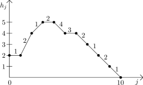
Figure 1: An ordered forest of two increasing ordered trees on the vertex set $[10]$, and its image under the bijection. We put the label $\xi_{j}$ above the step $s_{j}$.

Interpretation of the heights $\bm{h_{j}}$. Recall that $r_{j}$ is the number of trees in $F$ that contain at least one of the vertices $\{1,\ldots,j\}$. We then claim:

Lemma 3.3.

For $1\leq j\leq n$, the height $h_{j}=k+\sum_{i=1}^{j}s_{i}$ has the following interpretations:

• $h_{j}$ is the number of children of the vertices $\{1,\ldots,j\}$ whose labels are $>j$, plus $k-r_{j}$.

• $h_{j-1}$ is the number of children of the vertices $\{1,\ldots,j-1\}$ whose labels are $>j$, plus $k+1-r_{j}$. That is, $h_{j-1}$ is the level of the vertex $j$ as given in Definition 3.1.

In particular, $h_{j}>k-r_{j}$ whenever $j$ is not the highest-numbered vertex of its tree, and $h_{j}\geq k-r_{j}$ always.

Proof. By induction on $j$. For the base case $j=1$, the claims are clear since $r_{1}=1$, $h_{0}=k$ and $h_{1}=k+\deg(1)-1$.

For $j>1$, the vertex $j$ is either the child of another node, or the root of a tree. We consider these two cases separately:

(i) Suppose that $j$ is the child of another node (obviously numbered ${\leq j-1}$). By the inductive hypothesis (a), $h_{j-1}$ is the number of children of the vertices ${\{1,\ldots,j-1\}}$ whose labels are $\geq j$, plus $k-r_{j-1}$; and since one of these children is $j$, it follows that $h_{j-1}-1$ is the number of children of the vertices $\{1,\ldots,j-1\}$ whose labels are $>j$, plus $k-r_{j-1}$. Now vertex $j$ has $\deg(j)$ children, all of which have labels $>j$; so $h_{j}=h_{j-1}+s_{j}=h_{j-1}-1+\deg(j)$ is the number of children of the vertices $\{1,\ldots,j\}$ whose labels are $>j$, plus $k-r_{j-1}$. Since $r_{j}=r_{j-1}$, the preceding two sentences prove claims (b) and (a), respectively.

(ii) Suppose that $j$ is a root. By the inductive hypothesis (a), $h_{j-1}$ is the number of children of the vertices $\{1,\ldots,j-1\}$ whose labels are $\geq j$, plus $k-r_{j-1}$; and since $j$ is not one of these children, it follows that $h_{j-1}$ is also the number of children of the vertices $\{1,\ldots,j-1\}$ whose labels are $>j$, plus $k-r_{j-1}$. Now vertex $j$ has $\deg(j)$ children, all of which have labels $>j$; so $h_{j}=h_{j-1}+\deg(j)-1$ is the number of children of the vertices $\{1,\ldots,j\}$ whose labels are $>j$, plus $k-r_{j-1}-1$. Since $r_{j}=r_{j-1}+1$, the preceding two sentences prove claims (b) and (a), respectively. $\square$

It follows from Lemma 3.3(b) that $h_{0},\ldots,h_{n-1}\geq 1$ and $h_{n}=0$. So the path $\omega$ is indeed a reversed partial Łukasiewicz path from $(0,k)$ to $(n,0)$, which reaches level 0 only at the last step.

Corollary 3.4.

$\xi_{j}\leq h_{j-1}$.

Proof. By Lemma 3.3(b), the number of vertices $>j$ that are children of ${\{1,\ldots,j-1\}}$ is $h_{j-1}-(k+1-r_{j})$. The number of vertices $>j$ that are roots is at most $k-r_{j}$ (since any tree containing a vertex $\leq j$ necessarily has its root $\leq j$). So $\xi_{j}\leq 1+h_{j-1}-(k+1-r_{j})+(k-r_{j})=h_{j-1}$. $\square$

The inverse bijection. We claim that this mapping $F\mapsto(\omega,\xi)$ is a bijection from the set of ordered forests of increasing ordered trees on the vertex set $[n]$ with $k$ components to the set of labeled reversed partial Łukasiewicz paths from $(0,k)$ to $(n,0)$ that reach level 0 only at the last step, with integer labels satisfying $1\leq\xi_{j}\leq h_{j-1}$. To prove this, we explain the inverse mapping.

Given a labeled reversed partial Łukasiewicz path $(\omega,\xi)$, where $\omega$ reaches level 0 only at the last step, and $1\leq\xi_{j}\leq h_{j-1}$ for all $j$, we build up the ordered forest $F$ vertex-by-vertex: after stage $j$ we will have an ordered forest $F_{j}$ in which some of the vertices are labeled $1,\ldots,j$ and some others are unnumbered “vacant slots”. The starting forest $F_{0}$ has $k$ singleton components, each of which is a vacant slot (these components are of course ordered). We now “read” the path step-by-step, from $j=1$ through $j=n$. When we read a step $s_{j}$ with label $\xi_{j}$, we insert a new vertex $j$ into one of the vacant slots of $F_{j-1}$: namely, the $\xi_{j}$th vacant slot in the depth-first-search order of $F_{j-1}$. We also create $s_{j}+1$ new vacant slots that are children of $j$. This defines $F_{j}$. Since $F_{0}$ has $k=h_{0}$ vacant slots, and at stage $j$ we remove one vacant slot and add $s_{j}+1$ new ones, it follows by induction that $F_{j}$ has $h_{j}$ vacant slots. (In particular, the placement of the vertex $j$ into the $\xi_{j}$th vacant slot of $F_{j-1}$ is well-defined, since $1\leq\xi_{j}\leq h_{j-1}$ by hypothesis.) Since by hypothesis the path $\omega$ satisfies $h_{0},\ldots,h_{n-1}\geq 1$ and $h_{n}=0$, it follows that each forest $F_{0},\ldots,F_{n-1}$ has at least one vacant slot, while the forest $F_{n}$ has no vacant slot. We define $F=F_{n}$.

It is fairly clear that this insertion algorithm defines a map $(\omega,\xi)\mapsto F$ that is indeed the inverse of the mapping $F\mapsto(\omega,\xi)$ defined previously: this follows from the proof of Lemma 3.3 and the definition of the insertion algorithm.

Computation of the weights. We want to enumerate ordered forests of increasing ordered trees on the vertex set $[n]$ with $k$ components, in which each vertex at level $L$ with $i$ children gets a weight $\phi_{i}^{[L]}$. We use the bijection to push these weights from the forests to the labeled reversed partial Łukasiewicz paths. Given a forest $F$, each vertex $j\in[n]$ contributes a weight $\phi_{\deg(j)}^{[{\rm lev}(j)]}$. Under the bijection, this vertex is mapped to a step $s_{j}=\deg(j)-1$ from height $h_{j-1}={\rm lev}(j)$ to height $h_{j}=h_{j-1}+s_{j}$. Therefore, the weight in the labeled path $(\omega,\xi)$ corresponding to this vertex is $\phi_{s_{j}+1}^{[h_{j-1}]}$, and the weight of the labeled path $(\omega,\xi)$ is the product of these weights over $1\leq j\leq n$.

Now we sum over the labels $\xi$ to get the total weight for each path $\omega$: summing over $\xi_{j}$ gives a factor $h_{j-1}$. Therefore, the weight in the reversed partial Łukasiewicz path for a step $s$ ($-1\leq s<\infty$) starting from height $h$ will be

$$W(s,h)\;=\;h\,\phi_{s+1}^{[h]}\;.$$ (3.5)

Note that $W(s,0)=0$; this implements automatically the constraint that the reversed partial Łukasiewicz path is not allowed to reach level 0 before the last step.

We now want to read the path $\omega$ backwards, so that it becomes an ordinary partial Łukasiewicz path ${\widehat{\omega}}$ from $(0,0)$ to $(n,k)$. A step $s$ starting at height $h$ in $\omega$ becomes a step $s^{\prime}=-s$ starting at height $h^{\prime}=h+s$ in ${\widehat{\omega}}$. Therefore, in the ordinary partial Łukasiewicz path ${\widehat{\omega}}$, the weight will be

$$W^{\prime}(s^{\prime},h^{\prime})\;=\;(h^{\prime}+s^{\prime})\,\phi_{1-s^{\prime}}^{[h^{\prime}+s^{\prime}]}\;.$$ (3.6)

That is, a step from height $i$ to height $j$ gets a weight

$$p^{\rm ord}_{ij}\;=\;W(j-i,i)\;=\;j\,\phi_{i-j+1}^{[j]}\;.$$ (3.7)

(Note that $p^{\rm ord}_{i0}=0$, i.e. steps to level 0 are forbidden.) Then $P^{\rm ord}=(p^{\rm ord}_{ij})_{i,j\geq 0}$ is the production matrix for the triangle $(k!\,{\widehat{L}}_{n,k}({{\widehat{\vphantom{t}\smash{\bm{\phi}}\mkern 3.0mu}\mkern-3.0mu}{}}))_{n,k\geq 0}$ that enumerates ordered forests. This proves Proposition 3.2(a).

We then apply Lemma 2.2 with $B=\mathop{\rm diag}\nolimits\big{(}(1/k!)_{k\geq 0}\big{)}$, working temporarily in the ring ${\mathbb{Q}}[{{\widehat{\vphantom{t}\smash{\bm{\phi}}\mkern 3.0mu}\mkern-3.0mu}{}}]$. It follows that the production matrix $P$ for the triangle $({\widehat{L}}_{n,k}({{\widehat{\vphantom{t}\smash{\bm{\phi}}\mkern 3.0mu}\mkern-3.0mu}{}}))_{n,k\geq 0}$ is given by $P=B^{-1}P^{\rm ord}B$, which is precisely (3.2). This proves Proposition 3.2(b).

It also follows that the polynomial ${\widehat{L}}_{n,k}({{\widehat{\vphantom{t}\smash{\bm{\phi}}\mkern 3.0mu}\mkern-3.0mu}{}})$ has a factor $\phi_{0}^{[1]}\phi_{0}^{[2]}\cdots\phi_{0}^{[k]}$, since every partial Łukasiewicz path from $(0,0)$ to $(n,k)$ must have rises $0\to 1$, $1\to 2$, …, $k-1\to k$.

To prove Proposition 3.2(c), we apply Lemma 2.2 once again, this time with ${\widetilde{B}}=\mathop{\rm diag}\nolimits\big{(}(1/\phi_{0}^{[1]}\cdots\phi_{0}^{[k]})_{k\geq 0}\big{)}$, working temporarily in the ring ${\mathbb{Z}}[{{\widehat{\vphantom{t}\smash{\bm{\phi}}\mkern 3.0mu}\mkern-3.0mu}{}},{{\widehat{\vphantom{t}\smash{\bm{\phi}}\mkern 3.0mu}\mkern-3.0mu}{}}^{-1}]$. Of course the matrix elements of ${\widetilde{P}}={\widetilde{B}}^{-1}P{\widetilde{B}}$ lie in the subring ${\mathbb{Z}}[{{\widehat{\vphantom{t}\smash{\bm{\phi}}\mkern 3.0mu}\mkern-3.0mu}{}}]\subseteq{\mathbb{Z}}[{{\widehat{\vphantom{t}\smash{\bm{\phi}}\mkern 3.0mu}\mkern-3.0mu}{}},{{\widehat{\vphantom{t}\smash{\bm{\phi}}\mkern 3.0mu}\mkern-3.0mu}{}}^{-1}]$.

This completes the proof of Proposition 3.2. $\square$

Remark. The reasoning here using Lemma 2.2 corresponds, at the level of Łukasiewicz paths, to pairing each $\ell$-fall $i\to i-\ell$ ($\ell\geq 1$) with the corresponding rises $i-\ell\to i-\ell+1\to\ldots\to i$ and then transferring the weights (or part of the weights) from those rises to the $\ell$-fall (as was done in [37]). $\blacksquare$

Proof of Proposition 1.4(a).  Specialize Proposition 3.2(b) to the case $\phi_{i}^{[L]}=\phi_{i}$ for all $L$. $\square$

Note now that the triangular arrays ${\widehat{{\sf L}}}^{\rm ord}$, ${\widehat{{\sf L}}}$, ${\widetilde{{\sf L}}}$ are each of the form $\left[\begin{array}[]{c|c@{\hspace*{2mm}}c@{\hspace*{2mm}}c}1&0\hfil\hskip 5.69054pt&0\hfil\hskip 5.69054pt&\cdots\\ \hline\cr 0&\hfil\hskip 5.69054pt&\hfil\hskip 5.69054pt&\\ 0&\hfil\hskip 5.69054pt&L^{\wedge}\hfil\hskip 5.69054pt&\\[-2.84526pt] \vdots&\hfil\hskip 5.69054pt&\hfil\hskip 5.69054pt&\\ \end{array}\right]$. So it is of some interest to find the production matrix for the corresponding submatrices $L^{\wedge}$. Let us use the following notation: For any matrix $M=(m_{ij})_{i,j\geq 0}$, write $M^{\wedge}\stackrel{{\scriptstyle\rm def}}{{=}}\Delta M\Delta^{\rm T}$ for $M$ with its zeroth row and column removed. We then have:

Corollary 3.5.

Let ${{\widehat{\vphantom{t}\smash{\bm{\phi}}\mkern 3.0mu}\mkern-3.0mu}{}}=(\phi_{i}^{[L]})_{i\geq 0,\,L\geq 1}$ be indeterminates, and work in the ring $\mathbb{Z}[{{\widehat{\vphantom{t}\smash{\bm{\phi}}\mkern 3.0mu}\mkern-3.0mu}{}}]$. Define the lower-Hessenberg matrices $P^{\rm ord}$, $P$, ${\widetilde{P}}$ and the lower-triangular matrices ${\widehat{{\sf L}}}^{\rm ord}$, ${\widehat{{\sf L}}}$, ${\widetilde{{\sf L}}}$ as in Proposition 3.2. Then:

• $({\widehat{{\sf L}}}^{\rm ord})^{\wedge}=\phi_{0}^{[1]}\,{\mathcal{O}}((P^{\rm ord})^{\wedge})$.

• ${\widehat{{\sf L}}}^{\wedge}=\phi_{0}^{[1]}\,{\mathcal{O}}(P^{\wedge})$.

• ${\widetilde{{\sf L}}}^{\wedge}={\mathcal{O}}({\widetilde{P}}^{\wedge})$.

Proof. (a) By Proposition 3.2(a) we have ${\widehat{{\sf L}}}^{\rm ord}={\mathcal{O}}(P^{\rm ord})$. Now use Lemma 2.3 with $P,Q,c,A,B$ replaced by $(P^{\rm ord})^{\wedge},P^{\rm ord},\phi_{0}^{[1]},({\widehat{{\sf L}}}^{\rm ord})^{\wedge},{\widehat{{\sf L}}}^{\rm ord}$, respectively.

(b) and (c) are analogous. $\square$

Remark. In [37, sections 12.2 and 12.3] we considered the output matrix ${\widehat{{\sf L}}}^{\wedge}$ rather than ${\widehat{{\sf L}}}$, and therefore obtained the production matrix $P^{\wedge}$ rather than $P$. Also, in that paper we considered only the cases ${\bm{\phi}}={\bm{e}}$ and ${\bm{h}}$; but the proof for the generic case ${\bm{\phi}}$, given here, is completely analogous and indeed slightly simpler. $\square$

3.2 Identity for $\bm{B_{y}^{-1}PB_{y}}$ and proof of Proposition 1.4(b)

We now wish to prove the following identity:

Lemma 3.6 (Identity for $B_{y}^{-1}PB_{y}$).

Let ${\bm{\phi}}=(\phi_{i})_{i\geq 0}$ and $y$ be indeterminates, and work in the ring ${\mathbb{Z}}[{\bm{\phi}},y]$. Define the lower-Hessenberg matrix $P=(p_{ij})_{i,j\geq 0}$ by

$$p_{ij}\;=\;\begin{cases}0&\textrm{if $j=0$ or $j>i+1$}\\[2.84526pt] {\displaystyle{i!\over(j-1)!}}\,\phi_{i-j+1}&\textrm{if $1\leq j\leq i+1$}\end{cases}$$ (3.8)

and the unit-lower-triangular $y$-binomial matrix $B_{y}$ by

$$(B_{y})_{nk}\;=\;\binom{n}{k}\,y^{n-k}\;.$$ (3.9)

Let $\Delta=(\delta_{i+1,j})_{i,j\geq 0}$ be the matrix with 1 on the superdiagonal and 0 elsewhere. Then

$$B_{y}^{-1}PB_{y}\;=\;P(I+y\Delta^{\rm T})\;.$$ (3.10)

Proof. It is easy to see, using the Chu–Vandermonde identity, that $B_{y}B_{z}=B_{y+z}$ and hence that $B_{y}^{-1}=B_{-y}$. Therefore

$$(B_{y}^{-1}PB_{y})_{ij}\;=\;\sum_{k,\ell}(-1)^{i+k}\,{i!\over k!\,(i-k)!}\,y^{i-k}\>{k!\over(\ell-1)!}\,\phi_{k-\ell+1}\>{\ell!\over j!\,(\ell-j)!}\,y^{\ell-j}\;.$$ (3.11)

Then the coefficient of $\phi_{m}$ in this is (setting $k=\ell+m-1$)

$$&\!\!\!\![\phi_{m}]\,(B_{y}^{-1}PB_{y})_{ij}\;=\;(-1)^{i+m-1}\,{i!\over j!}\,y^{i-j+1-m}\sum_{\ell}(-1)^{\ell}\,{\ell\over(i-\ell-m+1)!\,(\ell-j)!}\qquad\\ \\ \qquad=\;(-1)^{i+m-1}\,{i!\over j!\,(i-j+1-m)!}\,y^{i-j+1-m}\sum_{\ell}(-1)^{\ell}\,\ell\,\binom{i-j+1-m}{\ell-j}\;.\\ {}$$ (3.12)

Now

$$\sum_{\ell}(-1)^{\ell}\,\binom{i-j+1-m}{\ell-j}\,x^{\ell}\;=\;(-x)^{j}\,(1-x)^{i-j+1-m}\;,$$ (3.13)

so that

$$\sum_{\ell}(-1)^{\ell}\,\ell\,\binom{i-j+1-m}{\ell-j}&={d\over dx}\bigl{[}(-x)^{j}\,(1-x)^{i-j+1-m}\bigr{]}\biggr{|}_{x=1}\\ =(-1)^{j}\,\bigl{[}j\delta_{m,i-j+1}\,-\,\delta_{m,i-j}\bigr{]}\;.$$ (3.14)

Substituting this into (LABEL:eq.proof.lemma.ByinvPBy.2.b) gives

$$(B_{y}^{-1}PB_{y})_{ij}&={i!\over j!}\,\bigl{[}j\phi_{i-j+1}\,+\,y\phi_{i-j}\bigr{]}\\ =p_{ij}\,+\,yp_{i,j+1}\;,$$ (3.15)

which is precisely (3.10). $\square$

We can now prove Proposition 1.4(b):

Proof of Proposition 1.4(b).  By Proposition 1.4(a), the matrix $P$ defined in (1.8)/(3.8) is the production matrix for the generic Lah triangle ${\sf L}$. By Lemma 2.2, the production matrix for ${\sf L}B_{y}$ is then $B_{y}^{-1}PB_{y}$; and by Lemma 3.6 this equals $P(I+y\Delta^{\rm T})$. $\square$

3.3 Total positivity of the production matrix

We shall use the following general lemma:

Lemma 3.7.

Let $A=(a_{ij})_{i,j\geq 0}$ be a lower-triangular matrix with entries in a partially ordered commutative ring $R$, and let ${\bm{d}}=(d_{i})_{i\geq 1}$. Define the lower-triangular matrix $B=(b_{ij})_{i,j\geq 0}$ by

$$b_{ij}\;=\;d_{j+1}d_{j+2}\cdots d_{i}\,a_{ij}\;.$$ (3.16)

Then:

• If $A$ is TP_r and ${\bm{d}}$ are indeterminates, then $B$ is TP_r in the ring $R[{\bm{d}}]$ equipped with the coefficientwise order.

• If $A$ is TP_r and ${\bm{d}}$ are nonnegative elements of $R$, then $B$ is TP_r in the ring $R$.

Proof. (a) Let ${\bm{d}}=(d_{i})_{i\geq 1}$ be commuting indeterminates, and let us work in the ring $R[{\bm{d}},{\bm{d}}^{-1}]$ equipped with the coefficientwise order. Let $D=\mathop{\rm diag}\nolimits(1,\,d_{1},\,d_{1}d_{2},\,\ldots)$. Then $D$ is invertible, and both $D$ and $D^{-1}=\mathop{\rm diag}\nolimits(1,\,d_{1}^{-1},\,d_{1}^{-1}d_{2}^{-1},\,\ldots)$ have nonnegative elements. It follows that $B=DAD^{-1}$ is TP_r in the ring $R[{\bm{d}},{\bm{d}}^{-1}]$ equipped with the coefficientwise order. But the matrix elements $b_{ij}$ actually belong to the subring $R[{\bm{d}}]\subseteq R[{\bm{d}},{\bm{d}}^{-1}]$. So $B$ is TP_r in the ring $R[{\bm{d}}]$ equipped with the coefficientwise order.

(b) follows from (a) by specializing indeterminates. $\square$

Corollary 3.8.

Let $(\phi_{i}^{[L]})_{i\geq 0,\,L\geq 1}$ be elements of a partially ordered commutative ring $R$, with $\phi_{i}^{[L]}\stackrel{{\scriptstyle\rm def}}{{=}}0$ for $i<0$. Suppose that the lower-triangular matrix $\Phi=(\phi_{i-j}^{[j+1]})_{i,j\geq 0}$ is TP_r. Then the matrices $P^{\rm ord}$ and $P$ defined by (3.1)/(3.2) are also TP_r.

Proof. (a) We have $P^{\rm ord}=\Phi\Delta D$ where $D=\mathop{\rm diag}\nolimits\big{(}(j)_{j\geq 0}\big{)}$.

(b) Applying Lemma 3.7(b) with $A=\Phi$ and $d_{i}=i!$, we see that the lower-triangular matrix $P^{\prime}=(p^{\prime}_{ij})_{i,j\geq 0}$ with entries $p^{\prime}_{ij}=(i!/j!)\,\phi_{i-j}^{[j+1]}$ is TP_r. But then $P=P^{\prime}\Delta$ is also TP_r. $\square$

The doubly-indexed sequence $(\phi_{i}^{[L]})_{i\geq 0,\,L\geq 1}$ is very general, but precisely because of its generality it is somewhat difficult to work with: indeed, the corresponding matrix $\Phi$ is a completely arbitrary lower-triangular matrix, for which it may or may not be feasible to determine its total positivity. It is therefore of interest to consider specializations for which the total positivity may be proven more easily. One such specialization is the following: Let ${\bm{\phi}}=(\phi_{i})_{i\geq 0}$ and ${\mathbf{c}}=(c_{L})_{L\geq 1}$ be two sequences of indeterminates, and set $\phi_{i}^{[L]}=\phi_{i}c_{L}$; we denote this specialization by the shorthand ${{\widehat{\vphantom{t}\smash{\bm{\phi}}\mkern 3.0mu}\mkern-3.0mu}{}}={\bm{\phi}}{\mathbf{c}}$. We then have the following easy fact:

Lemma 3.9.

Let ${\bm{\phi}}=(\phi_{i})_{i\geq 0}$ be a sequence in a partially ordered commutative ring $R$, with $\phi_{i}\stackrel{{\scriptstyle\rm def}}{{=}}0$ for $i<0$, and let ${\bm{c}}=(c_{L})_{L\geq 1}$; and define the lower-triangular matrix $\Phi=(\phi_{i-j}c_{j+1})_{i,j\geq 0}$ Then:

• If ${\bm{\phi}}$ is Toeplitz-TP_r and ${\bm{c}}$ are indeterminates, then $\Phi$ is TP_r in the ring $R[{\mathbf{c}}]$ equipped with the coefficientwise order.

• If ${\bm{\phi}}$ is Toeplitz-TP_r and ${\bm{c}}$ are nonnegative elements of $R$, then $\Phi$ is TP_r in the ring $R$.

Proof. We have $\Phi=T_{\infty}({\bm{\phi}})\,\mathop{\rm diag}\nolimits\big{(}(c_{j+1})_{j\geq 0}\bigr{)}$. $\square$

By combining Lemma 3.9 and Corollary 3.8, we deduce, under the same hypotheses, the TP_r property for the production matrices $P^{\rm ord}$ and $P$ evaluated at ${{\widehat{\vphantom{t}\smash{\bm{\phi}}\mkern 3.0mu}\mkern-3.0mu}{}}={\bm{\phi}}{\mathbf{c}}$.

3.4 Generalization of Theorem 1.1(a,c)

We can now state and prove a generalization of Theorem 1.1(a,c):

Theorem 3.10 (Total positivity of the refined generic Lah polynomials).

Let ${{\widehat{\vphantom{t}\smash{\bm{\phi}}\mkern 3.0mu}\mkern-3.0mu}{}}=(\phi_{i}^{[L]})_{i\geq 0,\,L\geq 1}$ be elements of a partially ordered commutative ring $R$, with $\phi_{i}^{[L]}\stackrel{{\scriptstyle\rm def}}{{=}}0$ for $i<0$, such that the lower-triangular matrix $\Phi=(\phi_{i-j}^{[j+1]})_{i,j\geq 0}$ is TP_r. Then:

• The lower-triangular matrix ${\widehat{{\sf L}}}({{\widehat{\vphantom{t}\smash{\bm{\phi}}\mkern 3.0mu}\mkern-3.0mu}{}})=({\widehat{L}}_{n,k}({{\widehat{\vphantom{t}\smash{\bm{\phi}}\mkern 3.0mu}\mkern-3.0mu}{}}))_{n,k\geq 0}$ is TP_r.

• The sequence ${\widehat{\bm{L}}}^{\triangle}({{\widehat{\vphantom{t}\smash{\bm{\phi}}\mkern 3.0mu}\mkern-3.0mu}{}})=({\widehat{L}}_{n+1,1}({{\widehat{\vphantom{t}\smash{\bm{\phi}}\mkern 3.0mu}\mkern-3.0mu}{}}))_{n\geq 0}$ is Hankel-TP_r.

Proof. (a) By Corollary 3.8, the production matrix $P$ defined in (3.2) is TP_r. By Proposition 3.2(b), the corresponding output matrix is ${\widehat{{\sf L}}}={\mathcal{O}}(P)$. So Theorem 2.5 implies that ${\widehat{{\sf L}}}$ is TP_r.

(c) By Corollary 3.8, the matrix $P$ is TP_r; hence so is $P^{\wedge}=\Delta P\Delta^{\rm T}$. By Corollary 3.5(b), we have ${\widehat{{\sf L}}}^{\wedge}=\phi_{0}^{[1]}\,{\mathcal{O}}(P^{\wedge})$. So Theorem 2.8 implies that the zeroth column of ${\widehat{{\sf L}}}^{\wedge}$ is Hankel-TP_r. But that is precisely $({\widehat{L}}_{n+1,1}({{\widehat{\vphantom{t}\smash{\bm{\phi}}\mkern 3.0mu}\mkern-3.0mu}{}}))_{n\geq 0}$. $\square$

Remark. Since an arbitrary lower-triangular matrix $\Phi$ can be written in the form $\Phi=(\phi_{i-j}^{[j+1]})_{i,j\geq 0}$, it follows that $\Phi\mapsto{\widehat{{\sf L}}}({{\widehat{\vphantom{t}\smash{\bm{\phi}}\mkern 3.0mu}\mkern-3.0mu}{}})$ is a well-defined polynomial mapping of the lower-triangular matrices into themselves, which preserves total positivity of each order $r$. However, this mapping seems rather complicated, even when restricted to Toeplitz matrices $\Phi$ (see the comments in Section 7 below). It would be interesting to better understand this mapping from an algebraic point of view. $\blacksquare$

As an immediate consequence of Lemma 3.9 and Theorem 3.10, we have:

Corollary 3.11.

Let ${\bm{\phi}}=(\phi_{i})_{i\geq 0}$ be a sequence in a partially ordered commutative ring $R$, and let ${\mathbf{c}}=(c_{L})_{L\geq 1}$ be indeterminates. If ${\bm{\phi}}$ is Toeplitz-TP_r, then:

• The lower-triangular matrix ${\widehat{{\sf L}}}({\bm{\phi}},{\mathbf{c}})=({\widehat{L}}_{n,k}({\bm{\phi}}{\mathbf{c}}))_{n,k\geq 0}$ is TP_r in the ring $R[{\mathbf{c}}]$ equipped with the coefficientwise order.

• The sequence ${\widehat{\bm{L}}}^{\triangle}({\bm{\phi}},{\mathbf{c}})=({\widehat{L}}_{n+1,1}({\bm{\phi}}{\mathbf{c}}))_{n\geq 0}$ is Hankel-TP_r in the ring $R[{\mathbf{c}}]$ equipped with the coefficientwise order.

Proof of Theorem 1.1(a,c).  Specialize Corollary 3.11(a,c) to ${\mathbf{c}}={\bm{1}}$. $\square$

3.5 Completion of the proofs

Proof of Theorem 1.1(b).  Since the zeroth column of the matrix ${\sf L}B_{y}$ is given by the Lah polynomials $L_{n}({\bm{\phi}},y)$, Theorem 1.1(b) is an immediate consequence of Proposition 1.4(b), Corollary 3.8 and Theorem 2.8. $\square$

Proof of Corollary 1.2.  The Jacobi–Trudi identity [44, Theorem 7.16.1 and Corollary 7.16.2] expresses all the Toeplitz minors of ${\bm{e}}$ or ${\bm{h}}$ as skew Schur functions. Furthermore, every skew Schur function is a nonnegative linear combination of Schur functions (Littlewood–Richardson coefficients [44, Section 7.A1.3]). So the sequences ${\bm{e}}$ and ${\bm{h}}$ are Toeplitz-totally positive with respect to the Schur order. Corollary 1.2 is then an immediate consequence of Theorem 1.1. $\square$

Furthermore, by using Corollary 3.11 here in place of Theorem 1.1(a,c), we obtain a generalization of Corollary 1.2(a,c), whose precise statement we leave to the reader; and likewise for Corollary 1.3.

4 Differential operators for the multivariate Lah polynomials

4.1 Differential operator for positive type

In [37, Proposition 12.6] we gave expressions for the multivariate Eulerian polynomials of positive type in terms of the action of certain first-order linear differential operators. Translated to our current notation, we proved the following:

Proposition 4.1.

[37, Proposition 12.6]  For every integer ${r\geq 1}$, we have

$$L_{n,1}^{(r)+}({\mathbf{x}}) = \Bigl{(}{\mathcal{D}}_{r}\,+\,\sum_{i=1}^{r}x_{i}\Bigr{)}^{\!n-1}\>1\qquad\hbox{for $n\geq 1$}$$ (4.1)

$$L_{n,k}^{(r)+}({\mathbf{x}}) = \Bigl{(}{\mathcal{D}}_{r}\,+\,k\sum_{i=1}^{r}x_{i}\Bigr{)}L_{n-1,k}^{(r)+}({\mathbf{x}})\>+\>L_{n-1,k-1}^{(r)+}({\mathbf{x}})\>+\>\delta_{n0}\delta_{k0}\quad\hbox{for $n,k\geq 0$}\qquad$$ (4.2)

where

$${\mathcal{D}}_{r}\;=\;\sum_{i=1}^{r}\biggl{(}\!x_{i}\!\!\!\!\sum_{00112233\begin{array}[]{c}1\leq j\leq r\\ j\neq i\end{array}}\!\!\!\!\!\!x_{j}\!\biggr{)}\,{\partial\over\partial x_{i}}\;.$$ (4.3)

Now we would like to extend this to give a differential expression for the row-generating polynomials $L_{n}^{(r)+}({\bf x},y)$:

Proposition 4.2.

For every integer $r\geq 1$, we have:

$$L_{n}^{(r)+}({\bf x},y)\;=\;({\widetilde{\mathcal{D}}}_{r}+y)^{n}\>1\;,$$ (4.4)

where

$${\widetilde{\mathcal{D}}}_{r}\;=\;{\mathcal{D}}_{r}\>+\>\sum_{i=1}^{r}x_{i}y\,{\partial\over\partial y}\;.$$ (4.5)

and ${\mathcal{D}}_{r}$ is defined in (4.3).

Proof. Multiply (4.2) by $y^{k}$ and sum over $k$: the factor $k$ becomes $y\,\partial/\partial y$, and we have

$$L_{n}^{(r)+}({\mathbf{x}},y)\;=\;\Bigl{(}{\mathcal{D}}_{r}\,+\,\sum_{i=1}^{r}x_{i}y\,{\partial\over\partial y}\,+\,y\Bigr{)}L_{n-1}^{(r)+}({\mathbf{x}},y)\>+\>\delta_{n0}\delta_{k0}\;.$$ (4.6)

Iterating this yields (4.4). $\square$

4.2 Differential operator for negative type

Similarly, in [37, Proposition 12.26] we gave expressions for the multivariate Eulerian polynomials of negative type in terms of the action of certain first-order linear differential operators. Translated to our current notation, we proved the following:

Proposition 4.3.

[37, Proposition 12.26]  For every integer ${r\geq 1}$, we have

$$L_{n,1}^{(r)-}({\mathbf{x}}) = \Bigl{(}{\mathcal{D}}^{-}_{r}\,+\,\sum_{i=1}^{r}x_{i}\Bigr{)}^{\!n-1}\>1\qquad\hbox{for $n\geq 1$}$$ (4.7)

$$L_{n,k}^{(r)-}({\mathbf{x}}) = \Bigl{(}{\mathcal{D}}^{-}_{r}\,+\,k\sum_{i=1}^{r}x_{i}\Bigr{)}L_{n-1,k}^{(r)-}({\mathbf{x}})\>+\>L_{n-1,k-1}^{(r)-}({\mathbf{x}})\>+\>\delta_{n0}\delta_{k0}\quad\hbox{for $n,k\geq 0$}\qquad$$ (4.8)

where

$${\mathcal{D}}^{-}_{r}\;=\;\sum_{i=1}^{r}\biggl{(}\!x_{i}^{2}\>+\>x_{i}\sum_{j=1}^{r}x_{j}\!\biggr{)}\,{\partial\over\partial x_{i}}\;.$$ (4.9)

Now we would like to extend this to give a differential expression for the row-generating polynomials $L_{n}^{(r)-}({\bf x},y)$, analogously to what we did for the positive type. The result is:

Proposition 4.4.

For every integer $r\geq 1$, we have:

$$L_{n}^{(r)-}({\bf x},y)\;=\;({\widetilde{\mathcal{D}}}_{r}^{-}+y)^{n}\>1\;,$$ (4.10)

where

$${\widetilde{\mathcal{D}}}_{r}^{-}\;=\;{\mathcal{D}}^{-}_{r}\>+\>\sum_{i=1}^{r}x_{i}y\,{\partial\over\partial y}\;.$$ (4.11)

and ${\mathcal{D}}^{-}_{r}$ is defined in (4.9).

Proof. Identical to the proof of Proposition 4.2, but with ${\mathcal{D}}_{r}$ replaced by ${\mathcal{D}}^{-}_{r}$. $\square$

5 Proof of Theorem 1.5 by the Euler–Gauss recurrence method

In the Introduction we explained how, for the multivariate Lah polynomials of positive type, the matrix $B_{y}^{-1}PB_{y}=P(I+y\Delta^{\rm T})$, which is the production matrix for ${\sf L}B_{y}$, has the bidiagonal factorization (1.10); and we explained how this in turn implies, by virtue of (2.21), that the multivariate Lah polynomials of positive type $L_{n}^{(r)+}({\mathbf{x}},y)$ are given by an $r$-branched S-fraction with coefficients

$${\bm{\alpha}}\;=\;(\alpha_{i})_{i\geq r}\;=\;y,x_{1},\ldots,x_{r},y,2x_{1},\ldots,2x_{r},y,3x_{1},\ldots,3x_{r},\,\ldots\;,$$ (5.1)

as stated in Theorem 1.5.

In this section we would like to give a second (and completely independent) proof of Theorem 1.5, based on the Euler–Gauss recurrence method for proving continued fractions, generalized to $m$-S-fractions as in [37, Proposition 2.3]. Let us recall briefly the method: if $(g_{k}(t))_{k\geq-1}$ are formal power series with constant term 1 (with coefficients in some commutative ring $R$) satisfying a recurrence

$$g_{k}(t)-g_{k-1}(t)\;=\;\alpha_{k+m}t\,g_{k+m}(t)\qquad\hbox{for }k\geq 0$$ (5.2)

for some coefficients ${\bm{\alpha}}=(\alpha_{i})_{i\geq m}$ in $R$, then $g_{0}(t)/g_{-1}(t)=\sum_{n=0}^{\infty}S^{(m)}_{n}({\bm{\alpha}})\,t^{n}$, where $S^{(m)}_{n}({\bm{\alpha}})$ is the $m$-Stieltjes–Rogers polynomial evaluated at the specified values ${\bm{\alpha}}$.

As in [37, sections 12.2.4 and 12.3.4], we will apply this method with the choice $g_{-1}(t)=1$. We need to find series $(g_{k}(t))_{k\geq 0}$ with constant term 1 satisfying (5.2), where here $m=r$. Let us write $g_{k}(t)=\sum_{n=0}^{\infty}g_{k,n}\,t^{n}$ and define $g_{k,n}=0$ for $n<0$. Then (5.2) can be written as

$$g_{k,n}\,-\,g_{k-1,n}\;=\;\alpha_{k+r}\,g_{k+r,n-1}\qquad\hbox{for }k,n\geq 0\;.$$ (5.3)

Here are the required $g_{k,n}$:

Proposition 5.1 (Euler–Gauss recurrence for multivariate Lah polynomials of positive type).

Let ${\mathbf{x}}=(x_{1},\ldots,x_{r})$ be indeterminates; we work in the ring $R={\mathbb{Z}}[{\mathbf{x}}]$. Set $g_{k,n}=\delta_{n0}$ for $k<0$, and then define $g_{k,n}$ for $k,n\geq 0$ by the recurrence

$$g_{k,n}\;=\;\Bigl{(}{\widetilde{\mathcal{D}}}_{r}\,+\,\sum_{i=1}^{r}\alpha_{k+i}\Bigr{)}g_{k,n-1}\>+\>g_{k-r,n}$$ (5.4)

where ${\widetilde{\mathcal{D}}}_{r}$ is given by (4.5) and ${\bm{\alpha}}$ are given by

$${\bm{\alpha}}\;=\;(\alpha_{i})_{i\geq 0}\;=\;\underbrace{0,\ldots,0}_{\text{$r$ times}},y,x_{1},\ldots,x_{r},y,2x_{1},\ldots,2x_{r},y,3x_{1},\ldots,3x_{r},\,\ldots$$ (5.5)

or in detail

$$\alpha_{i}\;=\;\begin{cases}\Big{\lfloor}\displaystyle\frac{i}{r+1}\Big{\rfloor}\,x_{j+1}&\textrm{if $i\equiv j\bmod r\!+\!1$ with $0\leq j\leq r\!-\!1$}\\[8.53581pt] y&\textrm{if $i\equiv r\bmod r\!+\!1$}\end{cases}$$ (5.6)

Then:

• $g_{k,0}=1$ for all $k\in{\mathbb{Z}}$.
  

• $(g_{k,n})$ satisfies the recurrence (5.3) for all $k\geq-r$ and $n\geq 0$.
  

• $S^{(r)}_{n}({\bm{\alpha}})=g_{0,n}=({\widetilde{\mathcal{D}}}_{r}+y)^{n}\,1$.

Proof. (a) We see trivially using (5.4) that $g_{k,0}=1$ for all $k\in{\mathbb{Z}}$, i.e. $g_{k}(t)$ has constant term 1.

(b) We will now prove that the recurrence (5.3) holds. The proof will be by an outer induction on $k$ (in steps of $r$) in which we encapsulate an inner induction on $n$. The base cases $k=-r,\ldots,-1$ for the outer induction hold trivially because $g_{k,n}=g_{k-1,n}=\delta_{n0}$ for $k<0$ and $\alpha_{0},\ldots,\alpha_{r-1}=0$. We now assume that (5.3) holds for a given $k$ and all $n\geq 0$; we want to prove that it still holds when we replace $k$ by $k+r$, i.e. that

$$g_{k+r,n}\>-\>g_{k+r-1,n}\>-\>\alpha_{k+2r}\,g_{k+2r,n-1}\;=\;0\quad\hbox{for all $n\geq 0$}\;.$$ (5.7)

We will prove (5.7) by induction on $n$.

Clearly (5.7) holds for $n=0$ because $g_{k+r,0}=g_{k+r-1,0}=1$ [from part (a)] and $g_{k+2r,-1}=0$ (by definition of the $g$’s).

When $n>0$, we use (5.4) on each of the three $g$’s on the left-hand side of (5.7), giving

$$g_{k+r,n}&=\Bigl{(}{\widetilde{\mathcal{D}}}_{r}\,+\,\sum_{i=1}^{r}\alpha_{k+r+i}\Bigr{)}g_{k+r,n-1}\>+\>g_{k,n}\\ g_{k+r-1,n}=\Bigl{(}{\widetilde{\mathcal{D}}}_{r}\,+\,\sum_{i=1}^{r}\alpha_{k+r-1+i}\Bigr{)}g_{k+r-1,n-1}\>+\>g_{k-1,n}\\ \alpha_{k+2r}\,g_{k+2r,n-1}=\alpha_{k+2r}\,\Bigl{(}{\widetilde{\mathcal{D}}}_{r}\,+\,\sum_{i=1}^{r}\alpha_{k+2r+i}\Bigr{)}g_{k+2r,n-2}\>+\>\alpha_{k+2r}\,g_{k+r,n-1}\qquad$$ (5.8)

We can then rewrite the left-hand-side of (5.7) as

LHS of (5.7) $$= g_{k,n}-g_{k-1,n}-\alpha_{k+2r}g_{k+r,n-1}$$ (5.9)

$$\quad+\,\sum_{i=1}^{r}\alpha_{k+r+i}\,(g_{k+r,n-1}-g_{k+r-1,n-1}-\alpha_{k+2r}g_{k+2r,n-2})$$

$$\quad+\,{\widetilde{\mathcal{D}}}_{r}(g_{k+r,n-1}-g_{k+r-1,n-1})\>-\>\alpha_{k+2r}\,{\widetilde{\mathcal{D}}}_{r}g_{k+2r,n-2}$$

$$\quad-\,\sum_{i=1}^{r}(\alpha_{k+r-1+i}-\alpha_{k+r+i})\,g_{k+r-1,n-1}$$

$$\quad-\,\sum_{i=1}^{r}(\alpha_{k+2r+i}-\alpha_{k+r+i})\,\alpha_{k+2r}\,g_{k+2r,n-2}\;.$$

On the right-hand side of (5.9), the first line is

$$g_{k,n}-g_{k-1,n}-\alpha_{k+2r}g_{k+r,n-1}$$

$$\qquad=\;g_{k,n}-g_{k-1,n}-\alpha_{k+r}g_{k+r,n-1}+(\alpha_{k+r}-\alpha_{k+2r})g_{k+r,n-1}$$

$$\qquad=\;(\alpha_{k+r}-\alpha_{k+2r})g_{k+r,n-1}\;,$$ (5.10)

where the first equality is trivial and the second one comes from the induction hypothesis on $k$. The second line of (5.9) is zero by the induction hypothesis on $n$. The fourth line of (5.9) is a telescoping sum over $i$, yielding simply $-(\alpha_{k+r}-\alpha_{k+2r})\,g_{k+r-1,n-1}$. For the third line of (5.9), we use the fact that ${\widetilde{\mathcal{D}}}_{r}$ is a pure first-order differential operator; then the Leibniz rule implies that the third line equals

$${\widetilde{\mathcal{D}}}_{r}(g_{k+r,n-1}-g_{k+r-1,n-1})\>-\>\alpha_{k+2r}{\widetilde{\mathcal{D}}}_{r}g_{k+2r,n-2}$$

$$\qquad=\;{\widetilde{\mathcal{D}}}_{r}(g_{k+r,n-1}-g_{k+r-1,n-1}-\alpha_{k+2r}g_{k+2r,n-2})\>+\>g_{k+2r,n-2}{\widetilde{\mathcal{D}}}_{r}\alpha_{k+2r}$$

$$\qquad=\;g_{k+2r,n-2}{\widetilde{\mathcal{D}}}_{r}\alpha_{k+2r}\;,$$ (5.11)

where the last equality comes from the induction hypothesis on $n$. We now need to do a distinction of cases to compute ${\widetilde{\mathcal{D}}}_{r}\alpha_{k+2r}$. If $k+2r\equiv r\bmod r+1$, we have $\alpha_{k+2r}=y$, and so

$${\widetilde{\mathcal{D}}}_{r}\alpha_{k+2r}\;=\;{\widetilde{\mathcal{D}}}_{r}y\;=\;y\sum_{i=1}^{r}x_{i}\;=\;\alpha_{k+2r}\sum_{i=1}^{r}x_{i}\;.$$ (5.12)

On the other hand, if $k+2r\equiv j\bmod r+1$ with $j\neq r$, we then have $\alpha_{k+2r}=\lfloor\frac{k+2r}{r+1}\rfloor x_{j+1}$, and so

$${\widetilde{\mathcal{D}}}_{r}\alpha_{k+2r}\;=\;{\widetilde{\mathcal{D}}}_{r}\Bigl{(}\Bigl{\lfloor}\frac{k+2r}{r+1}\Bigr{\rfloor}x_{j+1}\Bigr{)}\;=\;\Bigl{\lfloor}\frac{k+2r}{r+1}\Bigr{\rfloor}x_{j+1}\!\!\!\!\sum_{00112233\begin{array}[]{c}1\leq i\leq r\\ i\neq j+1\end{array}}\!\!\!\!x_{i}\;=\;\alpha_{k+2r}\!\!\!\!\sum_{00112233\begin{array}[]{c}1\leq i\leq r\\ i\neq j+1\end{array}}\!\!\!\!x_{i}\;.$$ (5.13)

Finally, the fifth line of of (5.9) is

$$-\sum_{i=1}^{r}(\alpha_{k+2r+i}-\alpha_{k+r+i})\,\alpha_{k+2r}\,g_{k+2r,n-2}$$

$$\qquad=\;-\Bigl{(}\alpha_{k+r}-\alpha_{k+2r}+\sum_{i=1}^{r}(\alpha_{k+2r+i}-\alpha_{k+r+i-1})\Bigr{)}\alpha_{k+2r}\,g_{k+2r,n-2}\qquad$$ (5.14)

by a change of index $i\to i-1$ in the second sum. Again, we need to do a distinction of cases to compute the sum. If $k+2r\equiv r\bmod r+1$, we then have

$$\sum_{i=1}^{r}\left(\alpha_{k+2r+i}-\alpha_{k+r+i-1}\right)\;=\;\sum_{i=1}^{r}x_{i}$$ (5.15)

by definition of the $\alpha$’s; whereas when $k+2r\equiv j\bmod r+1$ with $j\neq r$, we have

$$\sum_{i=1}^{r}\left(\alpha_{k+2r+i}-\alpha_{k+r+i-1}\right)\;=\;\!\!\!\!\sum_{00112233\begin{array}[]{c}1\leq i\leq r\\ i\neq j+1\end{array}}\!\!\!\!x_{i}\;.$$ (5.16)

And we still have the term $-(\alpha_{k+r}-\alpha_{k+2r})\alpha_{k+2r}g_{k+2r,n-2}$. In both cases, the sum involving the $x_{i}$’s cancels between the third and fifth lines; therefore, all that remains of the third and fifth lines is $-(\alpha_{k+r}-\alpha_{k+2r})\alpha_{k+2r}g_{k+2r,n-2}$.

Now, adding all the lines gives

$$(\alpha_{k+r}-\alpha_{k+2r})\,(g_{k+r,n-1}-g_{k+r-1,n-1}-\alpha_{k+2r}g_{k+2r,n-2})\;,$$ (5.17)

which vanishes by the induction hypothesis on $n$. This concludes the inductive step in $n$ to prove (5.7), which in turn concludes the induction on $k$ and finishes the proof of part (b).

(c) Putting $k=0$ in (5.4) gives $g_{0,n}=({\widetilde{\mathcal{D}}}_{r}+y)g_{0,n-1}+\delta_{n0}$, which proves $g_{0,n}=({\widetilde{\mathcal{D}}}_{r}+y)^{n}\,1$; and this equals $L_{n}^{(r)+}({\mathbf{x}},y)$ by Proposition 4.2. On the other hand, starting from the recurrence (5.3) and applying the Euler–Gauss recurrence method [37, Proposition 2.3], we conclude that $g_{0,n}=S_{n}^{(r)}({\bm{\alpha}})$. $\square$

6 Multivariate Lah polynomials in terms of decorated set partitions

In this section we would like to interpret the multivariate Lah polynomials of positive type $L_{n}^{(r)+}({\mathbf{x}},y)$ as generating polynomials for partitions of the set $[n]$ in which each block is “decorated” with an additional structure, where the nature of this structure depends on the value of $r$.

For $r=1,2$ we observed already in the Introduction how this goes: for $r=1$ the additional structure is empty, while for $r=2$ it is a linear ordering on the block. More precisely:

Proposition 6.1.

The polynomial $L_{n}^{(1)+}(1,y)$ is the Bell polynomial $B_{n}(y)$, that is, the generating polynomial of set partitions of $n$ elements with a weight $y$ for each block.

More generally, $L_{n}^{(1)+}(x_{1},y)$ is the homogenized Bell polynomial $x_{1}^{n}B_{n}(y/x_{1})$.

Proof. By definition, the polynomial $L_{n}^{(1)+}(1,y)$ is the generating polynomial of unordered forests of increasing unary trees. Since, given a set of integer labels, there is only one way to increasingly label a unary tree, there is a natural bijection between increasing unary trees and sets of labels. An unordered forest of increasing unary trees is then an unordered collection of disjoint sets of integers, whose union is $[n]$. But this is nothing other than a set partition of $[n]$.

The final statement follows from the fact that $L_{n}^{(1)+}(x_{1},y)$ is homogeneous of degree $n$. $\square$

Proposition 6.2.

The polynomial $L_{n}^{(2)+}({\bm{1}};y)$ is the Lah polynomial $L_{n}(y)$, that is, the generating polynomial of set partitions of $n$ elements into any number of nonempty lists (= linearly ordered subsets), with a weight $y$ for each list.

More generally, the polynomial $L_{n}^{(2)+}(x_{1},x_{2};y)$ is the generating polynomial of partitions of the set $[n]$ into any number of nonempty lists, with a weight $y$ for each list, $x_{1}$ for each descent in a list, and $x_{2}$ for each ascent in a list.

Proof. By definition, the polynomial $L_{n}^{(2)+}(x_{1},x_{2};y)$ is the generating polynomial of unordered forests of increasing binary trees, with a weight $y$ for each root (or equivalently, each tree) and a weight $x_{1}$ (resp. $x_{2}$) for each left (resp. right) child. Now, a classical bijection [43, pp. 23–25] sends increasing binary trees to permutations. Since a permutation is the same thing as a list, applying this classical bijection to each tree of the forest maps bijectively an unordered forest of increasing binary trees to a set of lists whose union is $[n]$, where the number of trees in the forest equals the number of lists.

The second claim comes out naturally, as this classical bijection maps a left (resp. right) child of the tree to a descent (resp. ascent) in the resulting permutation. $\square$

This can be generalized to any positive integer $r$ by using the concept of Stirling permutation [23, 21, 35, 36] as discussed in [37, section 12.5]. Recall that a word ${\mathbf{w}}=w_{1}\cdots w_{L}$ on a totally ordered alphabet $\mathbb{A}$ is called a Stirling word if $i<j<k$ and $w_{i}=w_{k}$ imply $w_{j}\geq w_{i}$: that is, between any two occurrences of any letter $a$, only letters that are larger than or equal to $a$ are allowed. (Equivalently, between any two successive occurrences of the letter $a$, only letters that are larger than $a$ are allowed.) Now let $\mathbb{A}$ be a totally ordered alphabet of finite cardinality $\ell$, and let $r$ be a nonnegative integer; we denote by $r\mathbb{A}$ the multiset consisting of $r$ copies of each letter $a\in\mathbb{A}$. A permutation of $r\mathbb{A}$ is a word $w_{1}\cdots w_{r\ell}$ containing exactly $r$ copies of each letter $a\in\mathbb{A}$; it is called a Stirling permutation of $r\mathbb{A}$ if it is also a Stirling word.

Now let $n$ be a nonnegative integer. We define an $\bm{r}$-Stirling set partition of $[n]$ to be a set partition of $[n]$ in which each block $B$ is decorated by a Stirling permutation of $rB$, where the total order on $B$ is of course the one inherited from the usual total order on the integers. In particular, when $r=0$, the decoration is empty, and we get back to classical set partitions; and when $r=1$, we get a partition of the set $[n]$ in which each block is decorated by a permutation of the letters of that block, or in other words, a partition of the set $[n]$ into nonempty lists.

Proposition 6.3.

The polynomial $L_{n}^{(r)+}({\bm{1}},y)$ is the generating polynomial of $(r-1)$-Stirling set partitions of $[n]$, with a weight $y$ for each block.

More generally, the polynomial $L_{n}^{(r)+}({\mathbf{x}},y)$ is the generating polynomial of $(r-1)$-Stirling set partitions of $[n]$, with a weight $y$ for each block, a weight $x_{i}$ ($1\leq i\leq r-1$) for each time the $i$th occurrence of a letter is the end of a descent, and a weight $x_{r}$ for each time the last occurrence of a letter is the beginning of an ascent.

Proof. By definition, the polynomial $L_{n}^{(r)+}({\mathbf{x}},y)$ is the generating polynomial for unordered forests of increasing $r$-ary trees, with a weight $y$ for each root and a weight $x_{i}$ for each $i$-child. Now a classical bijection [21, 25, 28] (see also [37, section 12.5]) sends increasing $r$-ary trees on the vertex set $[n]$ to Stirling permutations of the multiset $(r-1)[n]$, such that:

• A vertex $j$ has a 1-child if and only if the first occurrence of the letter $j$ in the word ${\mathbf{w}}$ is the end of a descent.

• A vertex $j$ has an $r$-child if and only if the last occurrence of the letter $j$ in the word ${\mathbf{w}}$ is the beginning of an ascent.

• A vertex $j$ has an $i$-child ($2\leq i\leq r-1$) if and only if in the word ${\mathbf{w}}$, between the $(i-1)$st and $i$th occurrences of the letter $j$ there is a nonempty subword; or equivalently, the $(i-1)$st occurrence of the letter $j$ is the beginning of an ascent; or equivalently, the $i$th occurrence of the letter $j$ is the end of a descent.

Applying this bijection to each tree of the forest maps bijectively unordered forests of increasing $r$-ary trees on the vertex set $[n]$ to a collection of Stirling permutations of multisets $(r-1)B_{i}$, where the $B_{i}$ taken together form a partition of the set $[n]$. This collection is nothing other than an $(r-1)$-Stirling set partition of $[n]$. $\square$

7 Exponential generating functions

By using exponential generating functions together with the Lagrange inversion formula, we can obtain explicit expressions for the generic Lah polynomials $L_{n,k}({\bm{\phi}})$. The method is due to Bergeron, Flajolet and Salvy [4]; see also [5, Chapter 5, especially pp. 364–365] and [37, section 12.2.1]. We will use Lagrange inversion in the following form [22]: If $A(u)$ is a formal power series with coefficients in a commutative ring $R$ containing the rationals, then there exists a unique formal power series $f(t)$ with zero constant term satisfying

$$f(t)\;=\;t\,A(f(t))\;,$$ (7.1)

and it is given by

$$[t^{n}]\,f(t)\;=\;{1\over n}\,[u^{n-1}]\,A(u)^{n}\quad\hbox{for $n\geq 1$}\;;$$ (7.2)

and more generally, if $H(u)$ is any formal power series, then

$$[t^{n}]\,H(f(t))\;=\;{1\over n}\,[u^{n-1}]\,H^{\prime}(u)\,A(u)^{n}\quad\hbox{for $n\geq 1$}\;.$$ (7.3)

Let ${\bm{\phi}}=(\phi_{i})_{i\geq 0}$ and $y$ be indeterminates; we will employ formal power series with coefficients in ${\mathbb{Q}}[{\bm{\phi}}]$ or ${\mathbb{Q}}[{\bm{\phi}},y]$. Recall that $L_{n,k}({\bm{\phi}})$ is the generating polynomial for unordered forests of increasing ordered trees on $n$ total vertices with $k$ components, in which each vertex with $i$ children gets a weight $\phi_{i}$; in particular, $L_{n,1}({\bm{\phi}})$ is the generating polynomial for increasing ordered trees. And $L_{n}({\bm{\phi}},y)=\sum_{k=0}^{n}L_{n,k}({\bm{\phi}})\>y^{k}$ are the row-generating polynomials. Define now the exponential generating function for trees:

$$U(t)\;=\;\sum_{n=1}^{\infty}L_{n,1}({\bm{\phi}})\,{t^{n}\over n!}\;.$$ (7.4)

It is easy to see that the exponential generating function for $k$-component unordered forests is

$${U(t)^{k}\over k!}\;=\;\sum_{n=0}^{\infty}L_{n,k}({\bm{\phi}})\,{t^{n}\over n!}\;.$$ (7.5)

Multiplying this by $y^{k}$ and summing over $k$ then gives the exponential generating function for the row-generating polynomials:

$$e^{yU(t)}\;=\;\sum_{n=0}^{\infty}L_{n}({\bm{\phi}},y)\,{t^{n}\over n!}\;.$$ (7.6)

Here is the key step: standard enumerative arguments [4, Theorem 1] show that $U(t)$ satisfies the ordinary differential equation

$$U^{\prime}(t)\;=\;\Phi(U(t))\;,$$ (7.7)

where $\Phi(w)\stackrel{{\scriptstyle\rm def}}{{=}}\sum_{k=0}^{\infty}\phi_{k}w^{k}$ is the ordinary generating function for ${\bm{\phi}}$. At this point it is convenient to specialize to $\phi_{0}=1$; at the end we can restore the missing factors of $\phi_{0}$ by recalling that $L_{n,k}({\bm{\phi}})$ is homogeneous of degree $n$ in ${\bm{\phi}}$. (Alternatively, we could keep $\phi_{0}$ and work over the ring ${\mathbb{Q}}[{\bm{\phi}},\phi_{0}^{-1}]$ instead of ${\mathbb{Q}}[{\bm{\phi}}]$.) We can now rewrite the differential equation (7.7) as the implicit equation

$$t\;=\;\int\limits_{0}^{U(t)}{dw\over\Phi(w)}\;.$$ (7.8)

Introducing $\Psi(w)\stackrel{{\scriptstyle\rm def}}{{=}}1/\Phi(w)\stackrel{{\scriptstyle\rm def}}{{=}}1+\sum_{i=1}^{\infty}\psi_{i}w^{i}$, we then have

$$t\;=\;U(t)\,\widehat{\Psi}(U(t))\qquad\hbox{where}\qquad\widehat{\Psi}(z)\;=\;1+\sum_{i=1}^{\infty}{\psi_{i}\over i+1}\,z^{i}\;.$$ (7.9)

Solving $U(t)=t/\widehat{\Psi}(U(t))$ by Lagrange inversion (7.3) with $A(u)=1/\widehat{\Psi}(u)$ and $H(u)=u^{k}/k!$ gives

$$&L_{n,k}({\bm{\phi}})\Bigr{|}_{\phi_{0}=1}\;=\;n!\>[t^{n}]\,{U(t)^{k}\over k!}\;=\;{(n-1)!\over(k-1)!}\>[z^{n-k}]\,\widehat{\Psi}(z)^{-n}\\ \;=\;{(n-1)!\over(k-1)!}\!\!\sum_{00112233\begin{array}[]{c}l_{1},l_{2},\ldots\geq 0\\ \sum il_{i}=n-k\end{array}}\!\!\!\!\binom{-n}{-n-\sum l_{i},\,l_{1},\,l_{2},\,\ldots}\prod_{i=1}^{\infty}\Bigl{(}{\psi_{i}\over i+1}\Bigr{)}^{\!l_{i}}\\ \;=\;{(n-1)!\over(k-1)!}\!\!\sum_{00112233\begin{array}[]{c}l_{1},l_{2},\ldots\geq 0\\ \sum il_{i}=n-k\end{array}}\!\!(-1)^{\sum l_{i}}\,\binom{n+\sum l_{i}-1}{n-1,\,l_{1},\,l_{2},\,\ldots}\prod_{i=1}^{\infty}\Bigl{(}{\psi_{i}\over i+1}\Bigr{)}^{\!l_{i}}\,.\;{}$$ (7.10)

Example 7.1 (Forests of increasing multi-unary trees).

The multivariate Lah polynomials of negative type $L_{n,k}^{(r)-}(x_{1},\ldots,x_{r})=L_{n,k}({\bm{h}}(x_{1},\ldots,x_{r}))$ specialized to $r=1$ and $x_{1}=1$ — which count unordered forests of increasing multi-unary trees — correspond to $\phi={\bm{1}}$, hence $\psi_{1}=-1$ and $\psi_{i}=0$ for $i\geq 2$. It follows that in (LABEL:eq.bergeron.Zn.c) we have $l_{1}=n-k$ and $l_{i}=0$ for $i\geq 2$, hence

$$L_{n,k}({\bm{1}})\;=\;{(2n-k-1)!\over 2^{n-k}\,(n-k)!\,(k-1)!}\;.$$ (7.11)

These are a shifted version of the coefficients of the (reversed) Bessel polynomials [33, A001497]. $\blacksquare$

Example 7.2 ($r=\infty$).

If we consider $r$-ary or multi-$r$-ary trees and take $r\to\infty$, then after an appropriate rescaling we get $\phi_{i}=1/i!$ and $\Phi(w)=e^{w}$. Solving (7.7) gives $U(t)=-\log(1-t)$ and hence

$$L_{n,k}({\bm{\phi}})\;=\;{n!\over k!}\;[t^{n}]\,(-\log(1-t))^{k}\;=\;\genfrac{[}{]}{0.0pt}{}{n}{k}\;,$$ (7.12)

the Stirling cycle numbers [33, A132393]. $\blacksquare$

Final remark. Here (LABEL:eq.bergeron.Zn.c) gives a nice explicit expression for $L_{n,k}({\bm{\phi}})$, but it is in terms of the coefficients $\psi_{i}$ in $\Psi(w)=1/\Phi(w)$, not directly in terms of the ${\bm{\phi}}$. Indeed, if one computes from (LABEL:eq.bergeron.Zn.c) the polynomials $L_{n,k}({\bm{\phi}})$, one finds some coefficients that have modestly (but not hugely) large prime factors: for instance, one of the terms in $L_{11,1}({\bm{\phi}})$ is $24950808\,\phi_{1}^{2}\phi_{2}\phi_{3}^{2}$, where $24950808=2^{3}\cdot 3^{3}\cdot 115513$; and one of the terms in $L_{13,1}({\bm{\phi}})$ is $2318149824\,\phi_{1}^{3}\phi_{2}^{3}\phi_{3}$, where $2318149824=2^{6}\cdot 3\cdot 12073697$. This suggests that the polynomials $L_{n,k}({\bm{\phi}})$ might not have any simple explicit expression. Or alternatively, they might have a simple explicit expression, but with coefficients that are given by sums and not just by products. We leave it as an open problem to find such an expression. $\blacksquare$

8 Note Added: Exponential Riordan arrays

After completing this paper we realized that the key Proposition 1.4(a), which expresses the production matrix of the generic Lah triangle and which we proved combinatorially in Section 3.1 by bijection onto labeled partial Łukasiewicz paths, can also be proven algebraically by using the theory of exponential Riordan arrays [14, 13, 3]. Here we would like to present briefly this alternate proof.

Let $R$ be a commutative ring containing the rationals, and let $F(t)=\sum_{n=0}^{\infty}f_{n}t^{n}/n!$ and $G(t)=\sum_{n=1}^{\infty}g_{n}t^{n}/n!$ be formal power series with coefficients in $R$; we set $g_{0}=0$. Then the exponential Riordan array associated to the pair $(F,G)$ — or equivalently to the pair of sequences ${\bm{f}}=(f_{n})_{n\geq 0}$ and ${\bm{g}}=(g_{n})_{n\geq 1}$ — is the infinite lower-triangular matrix ${\mathcal{R}}[F,G]=({\mathcal{R}}[F,G]_{nk})_{n,k\geq 0}$ defined by

$${\mathcal{R}}[F,G]_{nk}\;=\;{n!\over k!}\>[t^{n}]\,F(t)G(t)^{k}\;.$$ (8.1)

That is, the $k$th column of ${\mathcal{R}}[F,G]$ has exponential generating function $F(t)G(t)^{k}/k!$. Please note that the diagonal elements of ${\mathcal{R}}[F,G]$ are ${\mathcal{R}}[F,G]_{nn}=f_{0}g_{1}^{n}$, so the matrix ${\mathcal{R}}[F,G]$ is invertible in the ring $R^{{\mathbb{N}}\times{\mathbb{N}}}_{\rm lt}$ of lower-triangular matrices if and only if $f_{0}$ and $g_{1}$ are invertible in $R$.

We shall use an easy but important result that is sometimes called the fundamental theorem of exponential Riordan arrays (FTERA):

Lemma 8.1 (Fundamental theorem of exponential Riordan arrays).

Let ${\bm{b}}=(b_{n})_{n\geq 0}$ be a sequence with exponential generating function $B(t)=\sum_{n=0}^{\infty}b_{n}t^{n}/n!$. Considering ${\bm{b}}$ as a column vector and letting ${\mathcal{R}}[F,G]$ act on it by matrix multiplication, we obtain a sequence ${\mathcal{R}}[F,G]{\bm{b}}$ whose exponential generating function is $F(t)\,B(G(t))$.

Proof. We compute

$$\sum_{k=0}^{n}{\mathcal{R}}[F,G]_{nk}\,b_{k}&=\sum_{k=0}^{\infty}{n!\over k!}\,[t^{n}]\,F(t)G(t)^{k}\,b_{k}\\ =n!\>[t^{n}]\>F(t)\sum_{k=0}^{\infty}b_{k}\,{G(t)^{k}\over k!}\\ =n!\>[t^{n}]\>F(t)\,B(G(t))\;.$$ (8.2)

$\square$

We can now determine the production matrix of an exponential Riordan array ${\mathcal{R}}[F,G]$:

Theorem 8.2 (Production matrices of exponential Riordan arrays).

Let $L$ be a lower-triangular matrix (with entries in a commutative ring $R$ containing the rationals) with invertible diagonal entries and $L_{00}=1$, and let $P=L^{-1}\Delta L$ be its production matrix. Then $L$ is an exponential Riordan array if and only if $P=(p_{nk})_{n,k\geq 0}$ has the form

$$p_{nk}\;=\;{n!\over k!}\>(z_{n-k}\,+\,k\,a_{n-k+1})$$ (8.3)

for some sequences ${\bm{a}}=(a_{n})_{n\geq 0}$ and ${\bm{z}}=(z_{n})_{n\geq 0}$ in $R$.

More precisely, $L={\mathcal{R}}[F,G]$ if and only if $P$ is of the form (8.3) where the ordinary generating functions $A(t)=\sum_{n=0}^{\infty}a_{n}t^{n}$ and $Z(t)=\sum_{n=0}^{\infty}z_{n}t^{n}$ are connected to $F(t)$ and $G(t)$ by

$$G^{\prime}(t)\;=\;A(G(t))\;,\qquad{F^{\prime}(t)\over F(t)}\;=\;Z(G(t))$$ (8.4)

or equivalently

$$A(t)\;=\;G^{\prime}(\bar{G}(t))\;,\qquad Z(t)\;=\;{F^{\prime}(\bar{G}(t))\over F(\bar{G}(t))}$$ (8.5)

where $\bar{G}(t)$ is the compositional inverse of $G(t)$.

Proof (mostly contained in [3, pp. 217–218]). Suppose that $L={\mathcal{R}}[F,G]$. The hypotheses on $L$ imply that $f_{0}=1$ and that $g_{1}$ is invertible in $R$; so $G(t)$ has a compositional inverse. Now let $P=(p_{nk})_{n,k\geq 0}$ be a matrix; its column exponential generating functions are, by definition, $P_{k}(t)=\sum_{n=0}^{\infty}p_{nk}\,t^{n}/n!$. Applying the FTERA to each column of $P$, we see that ${\mathcal{R}}[F,G]P$ is a matrix whose column exponential generating functions are $\big{(}F(t)\,P_{k}(G(t))\big{)}_{k\geq 0}$. On the other hand, $\Delta\,{\mathcal{R}}[F,G]$ is the matrix ${\mathcal{R}}[F,G]$ with its zeroth row removed and all other rows shifted upwards, so it has column exponential generating functions

$${d\over dt}\,\big{(}F(t)\,G(t)^{k}/k!\big{)}\;=\;{1\over k!}\>\Big{[}F^{\prime}(t)\,G(t)^{k}\>+\>k\,F(t)\,G(t)^{k-1}\,G^{\prime}(t)\Big{]}\;.$$ (8.6)

Comparing these two results, we see that $\Delta\,{\mathcal{R}}[F,G]={\mathcal{R}}[F,G]\,P$ if and only if

$$P_{k}(G(t))\;=\;{1\over k!}\>{F^{\prime}(t)\,G(t)^{k}\>+\>k\,F(t)\,G(t)^{k-1}\,G^{\prime}(t)\over F(t)}\;,$$ (8.7)

or in other words

$$P_{k}(t)\;=\;{1\over k!}\>\biggl{[}{F^{\prime}(\bar{G}(t))\over F(\bar{G}(t))}\,t^{k}\>+\>k\,t^{k-1}\,G^{\prime}(\bar{G}(t))\biggr{]}\;.$$ (8.8)

Therefore

$$p_{nk}&={n!\over k!}\>[t^{n}]\,\biggl{[}{F^{\prime}(\bar{G}(t))\over F(\bar{G}(t))}\,t^{k}\>+\>k\,t^{k-1}\,G^{\prime}(\bar{G}(t))\biggr{]}\\ ={n!\over k!}\>\biggl{[}[t^{n-k}]\>{F^{\prime}(\bar{G}(t))\over F(\bar{G}(t))}\>+\>k\,[t^{n-k+1}]\>G^{\prime}(\bar{G}(t))\biggr{]}\\ ={n!\over k!}\>(z_{n-k}\,+\,k\,a_{n-k+1})$$ (8.9)

where ${\bm{a}}=(a_{n})_{n\geq 0}$ and ${\bm{z}}=(z_{n})_{n\geq 0}$ are given by (8.5).

Conversely, suppose that $P=(p_{nk})_{n,k\geq 0}$ has the form (8.3). Define $F(t)$ and $G(t)$ as the unique solutions (in the formal-power-series ring $R[[t]]$) of the differential equations (8.4) with initial conditions $F(0)=1$ and $G(0)=0$. Then running the foregoing computation backwards shows that $\Delta\,{\mathcal{R}}[F,G]={\mathcal{R}}[F,G]\,P$. $\square$

Alternate Proof of Proposition 1.4(a). We use the expressions for the exponential generating functions of the generic Lah polynomials, which were determined in Section 7. From (7.4)/(7.5) we see that the generic Lah triangle ${\sf L}=(L_{n,k}({\bm{\phi}}))_{n,k\geq 0}$ is the exponential Riordan array ${\mathcal{R}}[F,G]$ with $F(t)=1$ and $G(t)=U(t)$. Comparing (8.4) with (7.7), we see that $A(t)=\Phi(t)$ and $Z(t)=0$. The production matrix (8.3) then becomes (1.8), which proves Proposition 1.4(a). $\square$

Remark. This proof shows that the generic Lah triangle ${\sf L}=(L_{n,k}({\bm{\phi}}))_{n,k\geq 0}$ is in fact the general exponential Riordan array ${\mathcal{R}}[F,G]$ of the “associated subgroup” $F=1$, expressed in terms of its $A$-sequence ${\bm{a}}={\bm{\phi}}$. In this way, the theory of the generic Lah triangle is equivalent to the theory of exponential Riordan arrays of the “associated subgroup” ${\mathcal{R}}[1,G]$, expressed in the combinatorial language of unordered forests of increasing ordered trees. It would be interesting to work out the combinatorial interpretation of exponential Riordan arrays ${\mathcal{R}}[F,G]$ with $F\neq 1$. $\blacksquare$

This algebraic proof of Proposition 1.4(a) is arguably much simpler than the combinatorial proof presented in Section 3.1. On the other hand, the combinatorial method seems to be more powerful: we do not see (at least at present) how to extend the algebraic proof to obtain the more general Proposition 3.2, which expresses the production matrix of the refined generic Lah triangle.

Appendix A Lah polynomials for $\bm{n\leq 7}$

In this appendix we report the generic Lah polynomials $L_{n,k}({\bm{\phi}})$ for $n\leq 7$ (specialized for simplicity to $\phi_{0}=1$). We also report the Lah symmetric functions $L_{n,k}^{(\infty)+}$ and $L_{n,k}^{(\infty)-}$ for $n\leq 7$ in terms of the monomial symmetric functions $m_{\lambda}$; from these the reader can easily reconstruct explicit expressions for the multivariate Lah polynomials $L_{n,k}^{(r)+}(x_{1},\ldots,x_{r})$ and $L_{n,k}^{(r)-}(x_{1},\ldots,x_{r})$ for any chosen value of $r$. The conversions from $e_{\lambda}$ or $h_{\lambda}$ to $m_{\lambda}$ were performed using the SymFun Mathematica package (version 3.1), developed by Curtis Greene and collaborators [24].

A.1 Generic Lah polynomials

$$L_{1,1}({\bm{\phi}}) = 1$$

$$L_{2,1}({\bm{\phi}}) = \phi_{1}$$

$$L_{2,2}({\bm{\phi}}) = 1$$

$$L_{3,1}({\bm{\phi}}) = \phi_{1}^{2}+2\phi_{2}$$

$$L_{3,2}({\bm{\phi}}) = 3\phi_{1}$$

$$L_{3,3}({\bm{\phi}}) = 1$$

$$L_{4,1}({\bm{\phi}}) = \phi_{1}^{3}+8\phi_{1}\phi_{2}+6\phi_{3}$$

$$L_{4,2}({\bm{\phi}}) = 7\phi_{1}^{2}+8\phi_{2}$$

$$L_{4,3}({\bm{\phi}}) = 6\phi_{1}$$

$$L_{4,4}({\bm{\phi}}) = 1$$

$$L_{5,1}({\bm{\phi}}) = \phi_{1}^{4}+22\phi_{1}^{2}\phi_{2}+16\phi_{2}^{2}+42\phi_{1}\phi_{3}+24\phi_{4}$$

$$L_{5,2}({\bm{\phi}}) = 15\phi_{1}^{3}+60\phi_{1}\phi_{2}+30\phi_{3}$$

$$L_{5,3}({\bm{\phi}}) = 25\phi_{1}^{2}+20\phi_{2}$$

$$L_{5,4}({\bm{\phi}}) = 10\phi_{1}$$

$$L_{5,5}({\bm{\phi}}) = 1$$

$$L_{6,1}({\bm{\phi}}) = \phi_{1}^{5}+52\phi_{1}^{3}\phi_{2}+136\phi_{1}\phi_{2}^{2}+192\phi_{1}^{2}\phi_{3}+180\phi_{2}\phi_{3}+264\phi_{1}\phi_{4}+120\phi_{5}$$

$$L_{6,2}({\bm{\phi}}) = 31\phi_{1}^{4}+292\phi_{1}^{2}\phi_{2}+136\phi_{2}^{2}+342\phi_{1}\phi_{3}+144\phi_{4}$$

$$L_{6,3}({\bm{\phi}}) = 90\phi_{1}^{3}+240\phi_{1}\phi_{2}+90\phi_{3}$$

$$L_{6,4}({\bm{\phi}}) = 65\phi_{1}^{2}+40\phi_{2}$$

$$L_{6,5}({\bm{\phi}}) = 15\phi_{1}$$

$$L_{6,6}({\bm{\phi}}) = 1$$

$$L_{7,1}({\bm{\phi}}) = \phi_{1}^{6}+114\phi_{1}^{4}\phi_{2}+720\phi_{1}^{2}\phi_{2}^{2}+272\phi_{2}^{3}+732\phi_{1}^{3}\phi_{3}+2304\phi_{1}\phi_{2}\phi_{3}+540\phi_{3}^{2}$$

$$\quad+\,1824\phi_{1}^{2}\phi_{4}+1248\phi_{2}\phi_{4}+1920\phi_{1}\phi_{5}+720\phi_{6}$$

$$L_{7,2}({\bm{\phi}}) = 63\phi_{1}^{5}+1176\phi_{1}^{3}\phi_{2}+1848\phi_{1}\phi_{2}^{2}+2436\phi_{1}^{2}\phi_{3}+1680\phi_{2}\phi_{3}+2352\phi_{1}\phi_{4}+840\phi_{5}$$

$$L_{7,3}({\bm{\phi}}) = 301\phi_{1}^{4}+1792\phi_{1}^{2}\phi_{2}+616\phi_{2}^{2}+1512\phi_{1}\phi_{3}+504\phi_{4}$$

$$L_{7,4}({\bm{\phi}}) = 350\phi_{1}^{3}+700\phi_{1}\phi_{2}+210\phi_{3}$$

$$L_{7,5}({\bm{\phi}}) = 140\phi_{1}^{2}+70\phi_{2}$$

$$L_{7,6}({\bm{\phi}}) = 21\phi_{1}$$

$$L_{7,7}({\bm{\phi}}) = 1$$

A.2 Lah symmetric functions of positive type

$$L_{1,1}^{(\infty)+} = 1$$

$$L_{2,1}^{(\infty)+} = m_{1}$$

$$L_{2,2}^{(\infty)+} = 1$$

$$L_{3,1}^{(\infty)+} = m_{2}+4m_{11}$$

$$L_{3,2}^{(\infty)+} = 3m_{1}$$

$$L_{3,3}^{(\infty)+} = 1$$

$$L_{4,1}^{(\infty)+} = m_{3}+11m_{21}+36m_{111}$$

$$L_{4,2}^{(\infty)+} = 7m_{2}+22m_{11}$$

$$L_{4,3}^{(\infty)+} = 6m_{1}$$

$$L_{4,4}^{(\infty)+} = 1$$

$$L_{5,1}^{(\infty)+} = m_{4}+66m_{22}+26m_{31}+196m_{211}+576m_{1111}$$

$$L_{5,2}^{(\infty)+} = 15m_{3}+105m_{21}+300m_{111}$$

$$L_{5,3}^{(\infty)+} = 25m_{2}+70m_{11}$$

$$L_{5,4}^{(\infty)+} = 10m_{1}$$

$$L_{5,5}^{(\infty)+} = 1$$

$$L_{6,1}^{(\infty)+} = m_{5}+302m_{32}+57m_{41}+1898m_{221}+848m_{311}+5244m_{2111}+14400m_{11111}$$

$$L_{6,2}^{(\infty)+} = 31m_{4}+906m_{22}+416m_{31}+2446m_{211}+6576m_{1111}$$

$$L_{6,3}^{(\infty)+} = 90m_{3}+510m_{21}+1350m_{111}$$

$$L_{6,4}^{(\infty)+} = 65m_{2}+170m_{11}$$

$$L_{6,5}^{(\infty)+} = 15m_{1}$$

$$L_{6,6}^{(\infty)+} = 1$$

$$L_{7,1}^{(\infty)+} = m_{6}+2416m_{33}+1191m_{42}+120m_{51}+28470m_{222}+13644m_{321}+3228m_{411}$$

$$\quad+\,75216m_{2211}+36240m_{3111}+197856m_{21111}+518400m_{111111}$$

$$L_{7,2}^{(\infty)+} = 63m_{5}+6006m_{32}+1491m_{41}+31794m_{221}+15624m_{311}+82152m_{2111}+211680m_{11111}$$

$$L_{7,3}^{(\infty)+} = 301m_{4}+6006m_{22}+2996m_{31}+15316m_{211}+38976m_{1111}$$

$$L_{7,4}^{(\infty)+} = 350m_{3}+1750m_{21}+4410m_{111}$$

$$L_{7,5}^{(\infty)+} = 140m_{2}+350m_{11}$$

$$L_{7,6}^{(\infty)+} = 21m_{1}$$

$$L_{7,7}^{(\infty)+} = 1$$

A.3 Lah symmetric functions of negative type

$$L_{1,1}^{(\infty)-} = 1$$

$$L_{2,1}^{(\infty)-} = m_{1}$$

$$L_{2,2}^{(\infty)-} = 1$$

$$L_{3,1}^{(\infty)-} = 3m_{2}+4m_{11}$$

$$L_{3,2}^{(\infty)-} = 3m_{1}$$

$$L_{3,3}^{(\infty)-} = 1$$

$$L_{4,1}^{(\infty)-} = 15m_{3}+25m_{21}+36m_{111}$$

$$L_{4,2}^{(\infty)-} = 15m_{2}+22m_{11}$$

$$L_{4,3}^{(\infty)-} = 6m_{1}$$

$$L_{4,4}^{(\infty)-} = 1$$

$$L_{5,1}^{(\infty)-} = 105m_{4}+250m_{22}+210m_{31}+380m_{211}+576m_{1111}$$

$$L_{5,2}^{(\infty)-} = 105m_{3}+195m_{21}+300m_{111}$$

$$L_{5,3}^{(\infty)-} = 45m_{2}+70m_{11}$$

$$L_{5,4}^{(\infty)-} = 10m_{1}$$

$$L_{5,5}^{(\infty)-} = 1$$

$$L_{6,1}^{(\infty)-} = 945m_{5}+3010m_{32}+2205m_{41}+5810m_{221}+4760m_{311}+9156m_{2111}+14400m_{11111}$$

$$L_{6,2}^{(\infty)-} = 945m_{4}+2590m_{22}+2100m_{31}+4130m_{211}+6576m_{1111}$$

$$L_{6,3}^{(\infty)-} = 420m_{3}+840m_{21}+1350m_{111}$$

$$L_{6,4}^{(\infty)-} = 105m_{2}+170m_{11}$$

$$L_{6,5}^{(\infty)-} = 15m_{1}$$

$$L_{6,6}^{(\infty)-} = 1$$

$$L_{7,1}^{(\infty)-} = 10395m_{6}+48160m_{33}+42525m_{42}+27720m_{51}+122010m_{222}+97860m_{321}$$

$$\quad+\,69300m_{411}+197904m_{2211}+158928m_{3111}+320544m_{21111}+518400m_{111111}$$

$$L_{7,2}^{(\infty)-} = 10395m_{5}+38430m_{32}+26775m_{41}+79170m_{221}+63000m_{311}+129528m_{2111}$$

$$\quad+\,211680m_{11111}$$

$$L_{7,3}^{(\infty)-} = 4725m_{4}+14350m_{22}+11340m_{31}+23660m_{211}+38976m_{1111}$$

$$L_{7,4}^{(\infty)-} = 1260m_{3}+2660m_{21}+4410m_{111}$$

$$L_{7,5}^{(\infty)-} = 210m_{2}+350m_{11}$$

$$L_{7,6}^{(\infty)-} = 21m_{1}$$

$$L_{7,7}^{(\infty)-} = 1$$

References

- [1] M. Aigner, Catalan-like numbers and determinants, J. Combin. Theory A 87, 33–51 (1999).
- [2] J.-C. Aval, Multivariate Fuss-Catalan numbers, Discrete Math. 308, 4660–4669 (2008).
- [3] P. Barry, Riordan Arrays: A Primer (Logic Press, County Kildare, Ireland, 2016).
- [4] F. Bergeron, P. Flajolet and B. Salvy, Varieties of increasing trees, in CAAP ’92, edited by J.-C. Raoult, Lecture Notes in Computer Science #581 (Springer-Verlag, Berlin, 1992), pp. 24–48.
- [5] F. Bergeron, G. Labelle and P. Leroux, Combinatorial Species and Tree-Like Structures (Cambridge University Press, Cambridge–New York, 1998).
- [6] G.W. Brumfiel, Partially Ordered Rings and Semi-Algebraic Geometry, London Mathematical Society Lecture Note Series #37 (Cambridge University Press, Cambridge–New York, 1979).
- [7] N.T. Cameron and J.E. McLeod, Returns and hills on generalized Dyck paths, J. Integer Seq. 19, article 16.6.1 (2016), 28 pp.
- [8] X. Chen, H. Liang and Y. Wang, Total positivity of Riordan arrays, European J. Combin. 46, 68–74 (2015).
- [9] X. Chen, H. Liang and Y. Wang, Total positivity of recursive matrices, Lin. Alg. Appl. 471, 383–393 (2015).
- [10] X. Chen and Y. Wang, Notes on the total positivity of Riordan arrays, Lin. Alg. Appl. 569, 156–161 (2019).
- [11] L. Comtet, Advanced Combinatorics: The Art of Finite and Infinite Expansions (Reidel, Dordrecht–Boston, 1974). [French original: Analyse Combinatoire, tomes I et II, Presses Universitaires de France, Paris, 1970.]
- [12] E. Deutsch, L. Ferrari and S. Rinaldi, Production matrices, Adv. Appl. Math. 34, 101–122 (2005).
- [13] E. Deutsch, L. Ferrari and S. Rinaldi, Production matrices and Riordan arrays, Ann. Comb. 13, 65–85 (2009).
- [14] E. Deutsch and L. Shapiro, Exponential Riordan arrays, handwritten lecture notes, Nankai University, 26 February 2004, available on-line at http://www.combinatorics.net/ppt2004/Louis%20W.%20Shapiro/shapiro.pdf
- [15] S.M. Fallat and C.R. Johnson, Totally Nonnegative Matrices (Princeton University Press, Princeton NJ, 2011).
- [16] P. Flajolet, Combinatorial aspects of continued fractions, Discrete Math. 32, 125–161 (1980).
- [17] E. Fusy and E. Guitter, Comparing two statistical ensembles of quadrangulations: A continued fraction approach, Ann. Inst. Henri Poincaré D 4, 125–176 (2017).
- [18] F.R. Gantmacher and M.G. Krein, Oscillation Matrices and Kernels and Small Vibrations of Mechanical Systems (AMS Chelsea Publishing, Providence RI, 2002). Based on the second Russian edition, 1950.
- [19] F. Gantmakher and M. Krein, Sur les matrices complètement non négatives et oscillatoires, Compositio Math. 4, 445–476 (1937).
- [20] A.L.L. Gao, M. Pétréolle, A.D. Sokal, A.L.B. Yang and B.-X. Zhu, Total positivity of a class of Riordan-like matrices, implying a class of non-triangular linear transforms that preserve Hankel-total positivity, in preparation.
- [21] I. Gessel, A note on Stirling permutations, unpublished manuscript, August 1978, cited in [35].
- [22] I.M. Gessel, Lagrange inversion, J. Combin. Theory A 144, 212–249 (2016).
- [23] I. Gessel and R.P. Stanley, Stirling polynomials, J. Combin. Theory A 24, 24–33 (1978).
- [24] C. Greene et al., A Mathematica package for manipulating symmetric functions, http://ww3.haverford.edu/math/cgreene/symfun.html
- [25] S. Janson, M. Kuba and A. Panholzer, Generalized Stirling permutations, families of increasing trees and urn models, J. Combin. Theory A 118, 94–114 (2011).
- [26] M. Josuat-Vergès, A -analog of Schläfli and Gould identities on Stirling numbers, Ramanujan J. 46, 483–507 (2018).
- [27] S. Karlin, Total Positivity (Stanford University Press, Stanford CA, 1968).
- [28] M. Kuba and A.L. Varvak, On path diagrams and Stirling permutations, preprint, arXiv:0906.1672v2 [math.CO] at arXiv.org.
- [29] T.Y. Lam, An introduction to real algebra, Rocky Mountain J. Math. 14, 767–814 (1984).
- [30] H. Liang, L. Mu and Y. Wang, Catalan-like numbers and Stieltjes moment sequences, Discrete Math. 339, 484–488 (2016).
- [31] I.G. Macdonald, Symmetric Functions and Hall Polynomials, 2nd ed. (Clarendon Press, Oxford, 1995).
- [32] M. Marshall, Positive Polynomials and Sums of Squares, Mathematical Surveys and Monographs #146 (American Mathematical Society, Providence RI, 2008).
- [33] The On-Line Encyclopedia of Integer Sequences, published electronically at http://oeis.org
- [34] R. Oste and J. Van der Jeugt, Motzkin paths, Motzkin polynomials and recurrence relations, Electron. J. Combin. 22, no. 2, #P2.8 (2015).
- [35] S.-K. Park, The -multipermutations, J. Combin. Theory A 67, 44–71 (1994).
- [36] S.-K. Park, Inverse descents of -multipermutations, Discrete Math. 132, 215–229 (1994).
- [37] M. Pétréolle, A.D. Sokal and B.-X. Zhu, Lattice paths and branched continued fractions: An infinite sequence of generalizations of the Stieltjes–Rogers and Thron–Rogers polynomials, with coefficientwise Hankel-total positivity, preprint (2018), arXiv:1807.03271 [math.CO] at arXiv.org.
- [38] A. Pinkus, Totally Positive Matrices (Cambridge University Press, Cambridge, 2010).
- [39] A. Prestel and C.N. Delzell, Positive Polynomials: From Hilbert’s 17th Problem to Real Algebra (Springer-Verlag, Berlin, 2001).
- [40] H. Prodinger, Returns, hills, and -ary trees, J. Integer Seq. 19, article 16.7.2 (2016), 8 pp.
- [41] A.D. Sokal, Coefficientwise total positivity (via continued fractions) for some Hankel matrices of combinatorial polynomials, talk at the Séminaire de Combinatoire Philippe Flajolet, Institut Henri Poincaré, Paris, 5 June 2014; transparencies available at http://semflajolet.math.cnrs.fr/index.php/Main/2013-2014
- [42] A.D. Sokal, Coefficientwise total positivity (via continued fractions) for some Hankel matrices of combinatorial polynomials, in preparation.
- [43] R.P. Stanley, Enumerative Combinatorics, vol. 1 (Wadsworth & Brooks/Cole, Monterey, California, 1986). Reprinted by Cambridge University Press, 1999.
- [44] R.P. Stanley, Enumerative Combinatorics, vol. 2 (Cambridge University Press, Cambridge–New York, 1999).
- [45] T.J. Stieltjes, Sur la réduction en fraction continue d’une série procédant selon les puissances descendantes d’une variable, Ann. Fac. Sci. Toulouse 3, H1–H17 (1889).
- [46] T.J. Stieltjes, Recherches sur les fractions continues, Ann. Fac. Sci. Toulouse 8, J1–J122 (1894) and 9, A1–A47 (1895). [Reprinted, together with an English translation, in T.J. Stieltjes, Œuvres Complètes/Collected Papers (Springer-Verlag, Berlin, 1993), vol. II, pp. 401–566 and 609–745.]
- [47] B.-X. Zhu, Log-convexity and strong -log-convexity for some triangular arrays, Adv. Appl. Math. 50, 595–606 (2013).
- [48] B.-X. Zhu, Some positivities in certain triangular arrays, Proc. Amer. Math. Soc. 142, 2943–2952 (2014).