Abstract

This paper is concerned with inverse acoustic source problems in an unbounded domain with dynamical boundary surface data of Dirichlet kind. The measurement data are taken at a surface far away from the source support. We prove uniqueness in recovering source terms of the form $f(x)g(t)$ and $f(x_{1},x_{2},t)h(x_{3})$, where $g(t)$ and $h(x_{3})$ are given and $x=(x_{1},x_{2},x_{3})$ is the spatial variable in three dimensions. Without these a priori information, we prove that the boundary data of a family of solutions can be used to recover general source terms depending on both time and spatial variables. For moving point sources radiating periodic signals, the data recorded at four receivers are prove sufficient to uniquely recover the orbit function. Simultaneous determination of embedded obstacles and source terms was verified in an inhomogeneous background medium using the observation data of infinite time period. Our approach depends heavily on the Laplace transform.

Keywords: Inverse source problems, Laplace transform, moving point source, uniqueness.

1 Introduction

Inverse source problems have significant applications in many scientific areas such as antenna synthesis and design, biomedical engineering, medical imaging and optical tomography. For a mathematical overview of various inverse source problems we refer to [22] by Isakov where uniqueness and stability are discussed. An application in the fields of inverse diffraction and near-field holography was presented in [16, Chapter 2.2.5].

The approaches of applying Carleman estimate [30] and unique continuation [39] for hyperbolic equations have been widely used in the literature, giving rise to uniqueness and stability results for inverse coefficient and inverse source problems with the dynamical data over a finite time; we refer to [1, 8, 21, 25, 41, 42] for an incomplete list. Recently, an inverse source problem for doubly hyperbolic equations arising from the nucleation rate reconstruction in the three-dimensional time cone model was analyzed in [32]. A Lipschitz stability result was proved for recovering the spatial component of the source term using interior data and an iterative thresholding algorithm (see also [26] with the final observation data) was tested. However, most of the above mentioned works dealt with recovery of time independent source terms. We refer to [9, 36, 2, 18] where specific time-dependent source terms for hyperbolic equations were considered and to [29] for the recovery of some class of space-time-dependent source terms in the parabolic equation on a wave guide. In the time-harmonic case, inverse source problems with multi-frequency data have been extensively investigated. The increasing stability analysis in recovering spatial-dependent source terms has been carried out from both theoretical and numerical points of view (see e.g., [3, 6, 4, 5, 7, 11, 31, 40]).

In the time domain, it is very natural to transform the wave scattering problem governed by hyperbolic equations into elliptic inverse problems in the Fourier or Laplace domain with multi-frequency data; see e.g. [24] for determining sound-hard and impedance obstacles in a homogeneous background medium. In [7], the time-domain analysis helps for deriving an increasing stability to time-harmonic inverse source problems via Fourier transform. The same idea was used in [2, 20, 19] for recovering spatial-dependent sources as well as moving source profiles and orbits in elastodynamics and electromagnetism. The aim of this paper is to analyze the acoustic counterpart with new uniqueness results. Specially, this paper concerns the following four inverse problems with a single boundary surface data:

1. Simultaneous determination of sound-soft obstacles and separable source terms in an inhomogeneous medium (Subsection 2.1).

2. Simultaneous determination of sound-soft obstacles and general time-dependent source terms from a family of solutions (Subsection 2.2).

3. Inverse moving point source problems from the data of four receivers (Subsection 3.1) .

4. Determination of source terms which are independent of one spatial variable (Subsection 3.2) .

The Laplace (Fourier) transform will be used to handle the above inverse problems 1, 2 and 4. We highlight the novelty of this paper as follows. First, we verify the unique determination of both embedded obstacles and spatial-dependent source terms in an inhomogeneous medium. Although the acoustically sound-soft obstacles are considered within this paper, the proof carries over to other reflecting boundary conditions for impenetrable scatterers in acoustics and elastodynamics (see Remark 2.2). Second, the data of a family of solutions are used to recover a general source which depends on both time and space variables; Thirdly, the data of a finite number of receivers are proven sufficient to determine the orbit of a moving point source which radiates periodic temporal signals. This differs from inverse moving source problems of [19], where compactly supported temporal functions were considered and Huygens’ principle was applied. Our uniqueness proof seems new and leads straightforwardly to a numerical algorithm. Finally, the argument for recovering source terms independent of one spatial variable has simplified the corresponding proof in linear elasticity contained in [18]. Note that, although the measurement data are taken on a spherical surface, our results carry over to other non-spherical surfaces straightforwardly. In particular, Theorem 2.1, 2.5 and 3.3 remain valid if the data are observed on any subset of a closed analytical surface with positive Lebesgue measure.

The remaining part of this paper is divided into three sections. In the subsequent Section 2, we consider simultaneous determination of sound-soft obstacles and source terms via the Laplace transform. Section 3 is devoted to the unique determination of time-dependent source terms in a homogeneous background medium, including inverse moving source problems. Some remarks and open questions will be concluded in Section 4.

2 Simultaneous determination of sound-soft obstacles and source terms

Consider the time-dependent acoustic wave propagation in an inhomogeneous background medium with an acoustic source outside a sound-soft obstacle modelled by (see Figure 1)

$$\frac{1}{c^{2}(x)}{\color[rgb]{0.000,0.000,0.000}\partial^{2}_{t}}u(x,t)-\triangle u(x,t)=F(x,t),\quad x\in\mathbb{R}^{3}\backslash\bar{D},\quad t>0,$$ (2.1)

where $c(x)$ is the wave speed, $u(x,t)$ denotes the wave field, $D\subset\mathbb{R}^{3}$ represents the region of the sound-soft obstacle and $F(x,t)$ is the acoustic source term. Together with the above governing equation, we impose the homogeneous initial conditions

$$u(x,0)=0,\quad\partial_{t}u(x,0)=0,\quad x\in\mathbb{R}^{3}\backslash\bar{D},$$ (2.2)

and the Dirichlet boundary condition on $\partial D$:

$$u(x,t)=0,\quad(x,t)\in\partial D\times\mathbb{R}^{+}.$$ (2.3)

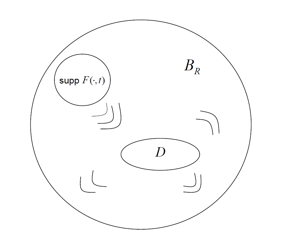
Figure 1: Radiation of a source in the exterior of a sound-soft obstacle $D$ in two dimensions. The inverse problem is to determine both the source term $F=F(x,t)$ and the obstacle $D$ from the displacement data measured on $\Gamma_{R}:=\{x\in\mathbb{R}^{3}:|x|=R\}{\color[rgb]{0.000,0.000,0.000}=\partial B_{R}}.$

Throughout this paper we assume that $D\subset B_{R}$ and that the source term $F(x,t)$ is compactly supported in $(B_{R}\backslash\overline{D})\times(0,T_{0})$. Here $B_{R}:=\{x\in\mathbb{R}^{3}:|x|<R\}$ and $R>0$, $T_{0}>0$ are constants. We denote the boundary of $B_{R}$ by $\Gamma_{R}:=\{x\in\mathbb{R}^{3}:|x|=R\}$. It is also supposed that $c\in L^{\infty}(\mathbb{R}^{3})$ satisfies

$$\exists c_{0}>0,\quad c(x)\geq c_{0}$$ (2.4)

and $\text{supp}(1-c)\subset B_{R}$, which means that the acoustic medium outside $B_{R}$ is homogeneous. We also assume that $\overline{\text{supp}(F(\cdot,t))}\cap\overline{D}=\emptyset$ for all $t>0$ and that $D$ is a $\mathcal{C}^{3}$-smooth domain with the connected exterior $\mathbb{R}^{3}\backslash\bar{D}$. Suppose that $F(x,t)\in L^{2}(0,T_{0};L^{2}(B_{R}\backslash\overline{D}))$. Then, the problem (2.1)-(2.3) admits a unique solution

$$u\in\mathcal{C}^{1}([0,+\infty);L^{2}(\mathbb{R}^{3}\backslash D))\cap\mathcal{C}([0,+\infty);H^{1}(\mathbb{R}^{3}\backslash D)).$$

The proof of this result can be carried out using the elliptic regularity properties of the Laplace operator (see [18, 17, 33, 34, 35]).

The goal of this section is to recover both the source term $F(x,t)$ and the embedded obstacle $D$ from the boundary surface data $\{u(x,t):~{}|x|=R,~{}t>0\}$ over an infinite time period. It is important to note that uniqueness in recovering time-dependent source terms is not true in general. A non-uniqueness example can be easily constructed in the absence of the obstacle $D$ (that is, $D=\emptyset$). In fact, let $\chi\in\mathcal{C}_{0}^{\infty}(B_{R}\times(0,T_{0}))\neq 0$ such that the function

$$F(x,t):=\frac{1}{c^{2}}{\color[rgb]{0.000,0.000,0.000}\partial^{2}_{t}}\chi-\triangle\chi,\quad(x,t)\in{\mathbb{R}}^{3}\times{\mathbb{R}}_{+}$$

does not vanish identically. Consider the inhomogeneous source problem

$$\begin{cases}\frac{1}{c(x)^{2}}{\color[rgb]{0.000,0.000,0.000}\partial^{2}_{t}}u(x,t)-\triangle u(x,t)=F(x,t),\quad x\in\mathbb{R}^{3}\times(0,+\infty),\\ u(x,0)=\partial_{t}u(x,0)=0,\quad x\in\mathbb{R}^{3}.\end{cases}$$ (2.5)

Clearly, from the uniqueness of solutions of (2.5) we conclude that $u=\chi$ is the unique solution. However, we have

$$u(x,t)=0,\quad|x|=R,\;t\in(0,+\infty),$$

due to the fact that $\text{supp}(\chi)\subset B_{R}\times(0,T_{0})$. This means that $F\neq 0$ is a non-radiation source and thus the surface data $\{u(x,t):|x|=R,~{}t>0\}$ usually do not allow the unique recovery of general source terms $F(x,t)$ satisfying $\text{supp}(F)\subset B_{R}\times(0,T_{0})$. It implies that there is no hope to prove uniqueness with a single measurement data. Facing this obstruction, we need to either know a certain a prior information of the source (see Subsections 2.1 and 3.2) or make use of extra data (see subsection 2.2) for recovering both time- and spatial-dependent source terms.

2.1 Spatial-dependent source terms in an inhomogeneous background medium

In this section we consider source terms of the form

$$F(x,t)=f(x)\;g(t),\quad x\in\mathbb{R}^{3}\backslash\bar{D},~{}t\in(0,\infty),$$ (2.6)

where $f\in L^{2}(B_{R}\backslash\overline{D})$ is the spatial-dependent source term to be determined and $g\in L^{2}(0,T_{0})$ is a given temporal function. We fix also $U$ an open and connected set of $\mathbb{R}^{3}$ such that $\overline{U}\subset B_{R}$.

Below we give a confirmative answer to the uniqueness issue of our inverse problem under proper assumptions on $supp(f_{j})$ and $D_{j}$.

Theorem 2.1.

Let $g\in L^{2}(0,T_{0})$ and let $c\in L^{\infty}(\mathbb{R})$ be such that $(1-c)$ is supported in $B_{R}$ and (2.4) is fulfilled. For $j=1,2$, let $D_{j}$ be an obstacle contained into $U$ and $f_{j}\in L^{2}(B_{R}\backslash\overline{D_{j}})$ satisfy ${\color[rgb]{0.000,0.000,0.000}\overline{supp(f_{j})}\subset B_{R}\backslash\overline{U}}$ and $U\setminus\overline{D_{j}}$ is connected. Here we assume that $f_{1},f_{2}$ are non-uniformly vanishing. Denote by $G$ the connected component of $U\backslash\overline{D_{1}\cup D_{2}}$ which can be connected to ${\mathbb{R}}^{3}\backslash\overline{B_{R}}$. We assume that there exists $\mathcal{O}$ an open and connected subset of $\mathbb{R}^{3}$ such that

$$\mathcal{O}\cap(\mathbb{R}^{3}\backslash B_{R})\neq\emptyset,\quad\mathcal{O}\cap G\neq\emptyset,\quad\mathcal{O}\cap\textrm{supp}(f_{1}-f_{2})=\emptyset.$$ (2.7)

Then, for $u_{j}$ solving (2.1)-(2.3) with $F(x,t)=f_{j}(x)g(t)$ and $D=D_{j}$, the condition

$$u_{1}(x,t)=u_{2}(x,t),\quad x\in\Gamma_{R},\,t>0,$$ (2.8)

implies $D_{1}=D_{2}$ and $f_{1}=f_{2}$.

If $f$ is known and $c(x)\equiv 1$, the unique determination of the sound-soft obstacle $D$ can be proved with the dynamical data over a finite time, following Isakov’s idea of using the sharp unique continuation for hyperbolic equations with analytic coefficients; see [23, Theorem 5.1]. If the obstacle $D$ is absent and the background medium is homogeneous, it was shown in [2, 20] via Huygens’ principle and Fourier transform that the boundary surface data can be used to uniquely determine $f$ in both elastodynamics and electromagnetism. Below we shall prove uniqueness in determining both $D$ and $f$ in an inhomogeneous medium. For this purpose, we need to apply the Laplace transform in place of the Fourier transform, because the strong Huygens’ principle is no longer valid.

Proof of Theorem 2.1. Obviously, $u_{1}$ and $u_{2}$ are solutions to

$$\begin{cases}\frac{1}{c^{2}(x)}{\color[rgb]{0.000,0.000,0.000}\partial^{2}_{t}}u_{j}(x,t)-\triangle u_{j}(x,t)=f_{j}(x)g(t),\quad&(x,t)\in\mathbb{R}^{3}\backslash\bar{D}_{j}\times\mathbb{R}^{+},\\ u_{j}(x,0)=\partial_{t}u_{j}(x,0)=0,\quad&x\in\mathbb{R}^{3}\backslash\bar{D}_{j},\\ u_{j}(x,t)=0,\quad&(x,t)\in\partial D_{j}\times\mathbb{R}^{+},\end{cases}$$ (2.9)

for $j=1,2$. By using standard argument for deriving energy estimates, we can prove that $u_{j}(x,t)$ $(j=1,2)$ has a long time behavior which is at most of polynomial type (see e.g., [18, Proposition 9]). This allows us to define the Laplace transform of $u:=u_{1}-u_{2}$ with respect to the time variable as following:

$$\hat{u}(x,s):=\int_{\mathbb{R}}u(x,t){\color[rgb]{0.000,0.000,0.000}{\rm e}}^{-st}{\rm d}t,\quad s>0,\quad x\in B_{R}.$$ (2.10)

Denote by $\tilde{D}$ the unbounded component of ${\mathbb{R}}^{3}\backslash\overline{D_{1}\cup D_{2}}$ and set $f:=f_{1}-f_{2}$. It then follows that

$$\begin{cases}\frac{1}{c^{2}(x)}{\color[rgb]{0.000,0.000,0.000}\partial^{2}_{t}}u(x,t)-\triangle u(x,t)=f(x)g(t),\quad&(x,t)\in\tilde{D}\times\mathbb{R}^{+},\\ u(x,0)=\partial_{t}u(x,0)=0,\quad&x\in\tilde{D},\\ u(x,t)=0,\quad&(x,t)\in\Gamma_{R}\times\mathbb{R}^{+}.\end{cases}$$

For notational convenience we set $\Omega_{1}:=B_{R}\backslash\bar{D}_{1}$, $\Omega_{2}:=B_{R}\backslash\bar{D}_{2}$ and $\Omega=B_{R}\cap\tilde{D}.$

Since $\widehat{{\color[rgb]{0.000,0.000,0.000}\partial^{2}_{t}}u}(x,s)=s^{2}\hat{u}(x,s)$ for all $s>0$ and the background wave speed $c(x)$ is known, the function $x\mapsto\hat{u}(x,s)$ solves

$$\begin{cases}\triangle\hat{u}(x,s)-\frac{s^{2}}{c^{2}(x)}\hat{u}(x,s)=f(x)\;\hat{g}(s)\quad&\text{in}\quad\tilde{D},\\ \hat{u}(x,s)=0\quad&\text{on}\quad\partial\tilde{D}.\end{cases}$$ (2.11)

Moreover, the uniqueness of solutions to the wave equation in the unbounded domain $|x|>R$ with the homogeneous Dirichlet boundary condition on $\Gamma_{R}\times(0,\infty)$, which can be justified via standard energy estimate (see e.g. [20] for a proof in electromagnetism), implies that $u(x,t)=0$ for $(x,t)\in(\mathbb{R}^{3}\backslash B_{R})\times(0,\infty)$. By Laplace transform, this gives the relation $\hat{u}(x,s)=0$ for $(x,s)\in(\mathbb{R}^{3}\backslash B_{R})\times(0,\infty)$. In view of (2.7), fixing $\mathcal{O}_{R}=\mathcal{O}\cap(\mathbb{R}^{3}\backslash B_{R})$, we deduce that, for all $s>0$, the restriction on $\mathcal{O}$ of $\hat{u}(\cdot,s)$ solves

$$\begin{cases}\triangle\hat{u}(x,s)-\frac{s^{2}}{c^{2}(x)}\hat{u}(x,s)=0\quad&x\in\mathcal{O},\\ \hat{u}(x,s)=0\quad&x\in\mathcal{O}_{R}.\end{cases}$$ (2.12)

Applying unique continuation results for elliptic equations (e.g. [14, Theorem 1.1] and [37, Theorem 1]), we deduce that

$$\hat{u}(x,s)=0\quad\text{for all}~{}x\in\mathcal{O}.$$

In particular, we have

$$\hat{u}(x,s)=0\quad\text{for all}~{}x\in\mathcal{O}\cap{\color[rgb]{0.000,0.000,0.000}G}$$

and we deduce that

$$\begin{cases}\triangle\hat{u}(x,s)-\frac{s^{2}}{c^{2}(x)}\hat{u}(x,s)=0\quad&x\in{\color[rgb]{0.000,0.000,0.000}G},\\ \hat{u}(x,s)=0\quad&x\in\mathcal{O}\cap{\color[rgb]{0.000,0.000,0.000}G}.\end{cases}$$ (2.13)

Applying again unique continuation results for elliptic equations and the fact that $O\cap({\mathbb{R}}^{3}\backslash B_{R})\neq\emptyset$, we deduce that

$$\hat{u}(x,s)=0\quad\text{for all}~{}x\in\overline{G}.$$ (2.14)

We first prove $D_{1}=D_{2}$. Assuming on the contrary that $D_{1}\neq D_{2}$, we shall derive a contraction as follows. Without loss of generality we may assume $D^{*}:=(U\backslash G)\backslash\overline{D}_{1}\neq\emptyset$. Then, using the fact that $\partial G\subset[\partial U\cup\partial(D_{1}\cup D_{2})]$ it holds that

$$\partial D^{*}\subset[\partial D_{1}\cup(\partial G\backslash\partial U)]\subset\partial D_{1}\cup(\partial G\cap\partial D_{2}).$$

On the other hand, from (2.14) we deduce that

$$\hat{u}_{1}(x,s)=\hat{u}_{2}(x,s)=0,\quad{\color[rgb]{0.000,0.000,0.000}x\in\partial G\cap\partial D_{2}},\ s>0.$$

Therefore, combining this with the fact that

$$\hat{u}_{1}(x,s)=0,\quad x\in\partial D_{1},\ s>0,$$

we deduce that $\hat{u}_{1}$ solves the boundary value problem

$$\begin{cases}\triangle\hat{u}_{1}(x,s)-\frac{s^{2}}{c^{2}(x)}\hat{u}_{1}(x,s)=0\quad&\text{in}~{}D^{*},\\ \hat{u}_{1}(x,s)=0\quad&\text{on}~{}\partial D^{*}\,{\color[rgb]{0.000,0.000,0.000},}\end{cases}$$

On the other hand, for all $s>0$, $0$ is not in the spectrum of the operator $-\triangle+\frac{s^{2}}{c^{2}(x)}$ with Dirichlet boundary condition on $D^{*}$ which is contained into $\left[\frac{s^{2}}{\|c\|_{L^{\infty}(D^{*})}},+\infty\right)$. Therefore, we have $\hat{u}_{1}(\cdot,s)\equiv 0$ in $D^{*}$. Applying unique continuation, we get $\hat{u}_{1}(\cdot,s)=0$ in $U\backslash\overline{D_{1}}$ for each $s>0$. In the same way, applying (2.7) we deduce that $\hat{u}_{1}(\cdot,s)=0$ in $\mathcal{O}$ and then that $\hat{u}_{1}(\cdot,s)=0$ on $\mathbb{R}^{3}\setminus\overline{B_{R}}$. Here we use the fact that $(\mathbb{R}^{3}\setminus\overline{B_{R}})\cap\mathcal{O}\neq\emptyset.$

For $R_{1}>R$, we fix $\tilde{\Omega}_{1}=B_{R_{1}}\backslash\overline{D_{1}}$ and $\Omega^{*}_{1}=B_{R_{1}}\backslash\overline{B_{R}}$. Then we have

$$\triangle{\color[rgb]{0.000,0.000,0.000}\hat{u}_{1}}(x,s)-\frac{s^{2}}{c^{2}(x)}{\color[rgb]{0.000,0.000,0.000}\hat{u}_{1}}(x,s)={\color[rgb]{0.000,0.000,0.000}f_{1}}(x)\;\hat{g}(s)\quad \text{in}\quad\tilde{\Omega}_{1},$$

and

$$\hat{u}_{1}(x,s)=0,\quad x\in\Omega^{*}_{1}$$

for every $s>0$. Denote by $\langle\cdot,\cdot\rangle$ the inner product in $L^{2}(\tilde{\Omega}_{1};c^{-2}dx)$, i.e.,

$$\langle u,v\rangle:=\int_{\tilde{\Omega}_{1}}c^{-2}(x)u(x)\bar{v}(x){\rm d}x,\quad u,v\in L^{2}(\tilde{\Omega}_{1}).$$

Denote by $\{\gamma_{l},\phi_{l,k}(x)\}_{l\in{\mathbb{N}}^{+},k\leq m_{l}}$ the eigenvalues and an associated orthonormal basis of eigenfunctions for the operator $-c^{2}(x)\triangle$ over $\tilde{\Omega}_{1}$ with the Dirichlet boundary condition acting on $L^{2}(\tilde{\Omega}_{1};c^{-2}dx)$. Here the eigenvalues satisfy the relation $0<\gamma_{1}<\gamma_{2}<\cdots<\gamma_{l}<\cdots$ and $\{\phi_{l,k}\}_{k=1}^{m_{l}}$ denotes the eigenspace associated with $\gamma_{l}$. In $\tilde{\Omega}_{1}$ we can represent the functions $c^{2}(x)f_{1}(x)$ and $\hat{u}_{1}(x,s)$ as

$$c^{2}(x)f_{1}(x) = \sum_{l\in\mathbb{N}^{+}}\sum_{k=1}^{m_{l}}\langle c^{2}f_{1},\phi_{l,k}\rangle\phi_{l,k}(x),\quad m_{l}\in{\mathbb{N}}^{+},$$

$$\hat{u}_{1}(x,s) = \hat{g}(s)\sum_{l\in\mathbb{N}^{+}}\frac{\sum_{k=1}^{m_{l}}\langle c^{2}f_{1},\phi_{l,k}\rangle\phi_{l,k}(x)}{s^{2}+\gamma_{l}},\quad s>0.$$ (2.15)

Note that the convergence of the series (2.15) can be understood in $L^{2}(\tilde{\Omega}_{1};c^{-2}dx)$. Since $g\in L^{2}(\mathbb{R}^{+})$ is supported in $[0,T_{0}]$ and does not vanish identically, there exists an interval $I\subset(0,+\infty)$ such that $|\hat{g}(s)|>0$ for all $s\in I$. Recalling that $\hat{u}_{1}(x,s)=0$ in $\Omega_{1}^{*}$, we have for all $s\in I$ that

$$\sum_{l\in\mathbb{N}^{+}}\frac{\sum_{k=1}^{m_{l}}\langle c^{2}f_{1},\phi_{l,k}\rangle\phi_{l,k}(x)}{s^{2}+\gamma_{l}}=0\quad\text{for}~{}\text{a.e.}~{}x\in\Omega^{*}_{1}.$$

On the other hand, the function

$$G(x,z):\quad z\rightarrow\sum_{l\in\mathbb{N}^{+}}\frac{\sum_{k=1}^{m_{l}}\langle c^{2}f_{1},\phi_{l,k}\rangle\phi_{l,k}(x)}{z+\gamma_{l}},\quad z\in\mathbb{C}\backslash\{-\gamma_{l}:l\in\mathbb{N}^{+}\}$$

can be regarded as a holomorphic function in the variable $z$ taking values in $L^{2}(\Omega^{*}_{1})$. Hence, by unique continuation for holomorphic functions we deduce that the condition

$$G(x,s^{2})={\color[rgb]{0.000,0.000,0.000}\hat{u}_{1}}(x,s)|_{x\in\Omega^{*}_{1}}=0\quad\text{for all}\quad s\in I$$

implies that

$$G(x,z)=0\quad\text{for all}\quad z\in\mathbb{C}\backslash\{-\gamma_{l}:l\in\mathbb{N}^{+}\}.$$

It follow that

$$(z+\gamma_{j})G(x,z)=0,\quad z\in\mathbb{C}\backslash\{-\gamma_{l}:l\in\mathbb{N}^{+}\},\quad j\in\mathbb{N}^{+}.$$ (2.16)

Therefore, letting $z\rightarrow-\gamma_{j}$ in (2.16) yields

$$\phi_{j}(x):=\sum_{k=1}^{m_{j}}\langle c^{2}f_{1},\phi_{j,k}\rangle\phi_{j,k}(x)=0\quad\text{for}\quad x\in\Omega^{*}_{1}.$$

On the other hand, we deduce that $\phi_{j}$ satisfies the elliptic equation

$$\triangle\phi_{j}(x)+\frac{\gamma_{j}}{c^{2}(x)}\phi_{j}(x)=0,\quad x\in\Omega^{*}_{1},$$

since $\phi_{l,k}$ are eigenfunctions. Applying the unique continuation of the Helmholtz equation gives

$$\sum_{k=1}^{m_{j}}\langle c^{2}f_{1},\phi_{j,k}\rangle\phi_{j,k}(x)=0\quad\text{for}\quad x\in\tilde{\Omega}_{1},$$

leading to the relations

$$\langle c^{2}f_{1},\phi_{j,k}\rangle=0,\quad k=1,2,\cdot\cdot\cdot,m_{j}.$$

Finally, by the arbitrariness of $j\in\mathbb{N}^{+}$ and the fact that $\text{supp}(f_{1})\subset\tilde{\Omega}_{1}$, we obtain

$$f_{1}=c^{-2}(c^{2}f_{1})\equiv 0\quad\text{for}~{}x\in\tilde{\Omega}_{1},$$

which is a contradiction to $f_{1}\neq 0$ in $\tilde{\Omega}_{1}$. Thus, we obtain $D_{1}=D_{2}$.

It remains to prove the coincidence of the source $f_{1}=f_{2}$. We shall deduce $f=f_{1}-f_{2}\equiv 0$ from the boundary value problem (2.11) in an open set $\tilde{\Omega}$ such that $\text{supp}(f)\subset\tilde{\Omega}\subset\subset\Omega$. It is easy to prove that $\hat{u}(x,s)$ vanishes in $\tilde{\Omega}\backslash\overline{\text{supp}(f)}$. Similarly to (2.15), we can represent $c^{2}(x)f(x),\hat{u}(x,s)$ in the form of (2.15) in $\tilde{\Omega}$. Consequently, following similar arguments in the first step we can obtain $f=0$ in $\tilde{\Omega}$ by making use of the vanishing of $u$ in ${\color[rgb]{0.000,0.000,0.000}\tilde{\Omega}\backslash\overline{\text{supp}(f)}}$. ∎

Remark 2.2.

(i) Assuming that $c\in\mathcal{C}^{1}(\mathbb{R}^{n})$, one can apply the local unique continuation results of [38, Theorem 1] in order to derive a global Holmgren uniqueness theorem similar to [27, Theorem 3.16] (see also [28, Theorem A.1.]). Combining this with the arguments used in [18, Theorem 2] it is possible to prove Theorem 2.1 in a more straightforward way. However, for more general coefficients $c\in L^{\infty}(\mathbb{R}^{n})$, it is not clear that [38, Theorem 1] holds true and we can not apply such arguments. In that sense, in contrast to [18, Theorem 2], the approach considered in Theorem 2.1 can be applied to equations with less regular coefficients.

(ii)The result of Theorem 2.1 carries over to other boundary conditions of the form

$$\partial_{\nu}u-a\partial_{t}u-bu=0\quad\mbox{on}\quad\partial D\times{\mathbb{R}}^{+},$$

where $a\geq 0$ and $b\geq 0$. The proof can be carried out by applying the Laplace transform with the variable $s=s_{1}+is_{2}\in{\mathbb{C}}^{+}$ such that $s_{1},s_{2}>0$; we refer to [24] by Isakov where uniqueness results for recovering impenetrable obstacles were discussed. Note that although the gap domain $D^{*}$ between two obstacles might be cuspidal and non-lipschitzian, the regularity assumption of $\partial D$ ensures that $\hat{u}(\cdot,s)\in H^{2}(B_{R}\backslash\overline{D})$ and the boundary $\partial D^{*}$ of the gap domain is piecewise smooth. Hence, the traces $\hat{u}(x,s)$ and $\partial_{\nu}\hat{u}(x,s)$ are well defined on ${\color[rgb]{0.000,0.000,0.000}\partial D^{*}}$. However, it remains unclear to us how to treat penetrable scatterers with transmission conditions on the interface.

(iii) The proof of Theorem 2.1 can be simplified if the background medium is homogeneous, i.e., $c(x)\equiv 1$ in ${\mathbb{R}}^{3}\backslash\overline{D}$. In fact, in a homogeneous medium the uniqueness proof can be reduced to verifying the vanishing of $f_{1}$ if

$$\triangle\hat{u}_{1}(x,s)-s^{2}\hat{u}_{1}(x,s)=\hat{g}(s)f_{1}(x), \quad x\in{\color[rgb]{0.000,0.000,0.000}\tilde{\Omega}_{1}},$$

$$\hat{u}_{1}(x,s)=\partial_{\nu}\hat{u}_{1}(x,s)(x,s)=0, \quad x\in\partial{\color[rgb]{0.000,0.000,0.000}\tilde{\Omega}_{1}}$$

for each $s>0$ and for some domain $\tilde{\Omega}_{1}$ containing ${\rm supp}(f_{1})$. Multiplying both sides of (2.2) by the test function $\varphi(x)={\color[rgb]{0.000,0.000,0.000}{\rm e}}^{sx\cdot d}$ with $d\in{\mathbb{R}}^{3}$, $|d|=1$ and integrating by parts over $B$ yield

$$\hat{g}(s)\int_{{\color[rgb]{0.000,0.000,0.000}\tilde{\Omega}_{1}}}f_{1}(x){\color[rgb]{0.000,0.000,0.000}{\rm e}}^{sx\cdot d}{\rm d}x=0\quad\mbox{for all}\quad s\in{\mathbb{R}}.$$ (2.17)

Clearly, $\hat{g}(z)$ and $\int_{{\color[rgb]{0.000,0.000,0.000}\tilde{\Omega}_{1}}}f_{1}(x){\color[rgb]{0.000,0.000,0.000}{\rm e}}^{zx\cdot d}{\rm d}x$ are both holomorphic functions with respect to the variable $z\in\mathbb{C}$. Using the assumption $g\neq 0$ it is easy to prove that $\int_{{\color[rgb]{0.000,0.000,0.000}\tilde{\Omega}_{1}}}f_{1}(x){\color[rgb]{0.000,0.000,0.000}{\rm e}}^{sx\cdot d}{\rm d}x=0$ for all $s\in\mathbb{R}$ and $|d|=1$. This implies that the Laplace transform of $f_{1}$ vanishes everywhere and hence $f_{1}\equiv 0$.

Consider the acoustic wave equation with a homogeneous source term and inhomogeneous initial conditions $v_{0}$ and $v_{1}$:

$$\begin{cases}\frac{1}{c^{2}(x)}{\color[rgb]{0.000,0.000,0.000}\partial^{2}_{t}}u(x,t)-\triangle u(x,t)=0,\quad&x=(x_{1},x_{2},x_{3})\in\mathbb{R}^{3}\backslash\bar{D},t>0,\\ u(x,0)=v_{0}(x),\partial_{t}u(x,0)=v_{1}(x),\quad&x\in\mathbb{R}^{3}\backslash D,\\ u(x,t)=0,\quad&(x,t)\in\partial D\times\mathbb{R}^{+}.\end{cases}$$ (2.18)

Applying the Laplace transform to $u$ and noting that $\widehat{{\color[rgb]{0.000,0.000,0.000}\partial^{2}_{t}}u}(x,s)=s^{2}\hat{u}(x,s)-v_{1}-sv_{0}$ yield the boundary value problem

$$\begin{cases}\triangle\hat{u}(x,s)-\frac{s^{2}}{c^{2}(x)}\hat{u}(x,s)=\frac{1}{c^{2}(x)}(sv_{0}(x)+v_{1}(x))\quad&\text{in}~{}R^{3}\backslash\bar{D},\\ \hat{u}(x,s)=0\quad&\text{on}~{}\partial D\,.\end{cases}$$

Following similar arguments as those in the proof of Theorem 2.1, we can determine simultaneously the obstacle $D$, the initial displacement $v_{0}$ and initial velocity $v_{1}$ from the radiated field $u$ measured on the surface $\Gamma_{R}\times\mathbb{R}^{+}$.

Corollary 2.3.

Let $c\in L^{\infty}(\mathbb{R})$ be such that $(1-c)$ is supported in $B_{R}$ and (2.4) is fulfilled. For $j=1,2$, let $D_{j}$ be an obstacle contained into $U$, $v_{j,0}\in H^{2}({\mathbb{R}}^{3}\backslash\overline{D})$ and $v_{j,1}\in H^{1}({\mathbb{R}}^{3}\backslash\overline{D})$ satisfy $\overline{supp(v_{j,0})}\cup\overline{supp(v_{j,1})}\subset B_{R}\backslash\overline{U}$ with $U\setminus\overline{D_{j}}$ connected. Here we assume that $v_{j,0}$, $v_{j,1}$, $j=1,2$, are non-uniformly vanishing. Assume also that there exists $\mathcal{O}$ an open and connected subset of $\mathbb{R}^{3}$ such that (2.7) is fulfilled with the last relation replaced by

$$\mathcal{O}\cap\textrm{supp}(v_{1,j}-v_{2,j})=\emptyset,\quad j=0,1.$$

Then, for $u_{j}$ solving (2.18) with $v_{0}=v_{j,0}$, $v_{1}=v_{j,1}$ and $D=D_{j}$, the condition

$$u_{1}(x,t)=u_{2}(x,t),\quad x\in\Gamma_{R},\,t>0,$$ (2.19)

implies $D_{1}=D_{2}$, $v_{1,0}=v_{2,0}$ and $v_{1,1}=v_{2,1}$.

Remark 2.4.

• Like Theorem 2.1, for $c\in\mathcal{C}^{1}(\mathbb{R}^{n})$ one can deduce and even improve Corollary 2.3 by using an approach based on unique continuation properties with arguments borrowed from [38, Theorem 1], [27, Theorem 3.11] and [18, Theorem 2]. However, since for $c\in L^{\infty}(\mathbb{R}^{n})$, it is not clear that [38, Theorem 1] holds true, we can not consider such approach. In that sense, in contrast to other similar results, Corollary 2.3 can be applied to equations with less regular coefficients $c$.
  

• The results of Theorem 2.1 and Corollary 2.3 hold true with a finite time observation data on $\Gamma_{R}\times(0,T)$ if $g(0)\neq 0$. In fact, by Duhamel’s principle, we may represent $u_{j}$ to the equation (2.9) as

  $$u_{j}(x,t)=\int_{0}^{t}g(t-s)\,v_{j}(x,s)\,ds,\qquad t\in(0,\infty),$$ (2.20)

  where $v_{j}$ solves the initial value problem of the homogeneous wave equation

  $$\begin{cases}\frac{1}{c^{2}(x)}{\color[rgb]{0.000,0.000,0.000}\partial^{2}_{t}}v_{j}(x,t)-\triangle v_{j}(x,t)=0,\quad&(x,t)\in\mathbb{R}^{3}\backslash\bar{D}_{j}\times\mathbb{R}^{+},\\ v_{j}(x,0)=0,\quad\partial_{t}v_{j}(x,0)=f_{j}(x),\quad&x\in\mathbb{R}^{3}\backslash\bar{D}_{j},\\ v_{j}(x,t)=0,\quad&(x,t)\in\partial D_{j}\times\mathbb{R}^{+}.\end{cases}$$

  If $g(0)\neq 0$, differentiating (2.20) and then applying the Grownwall inequality could lead to the relation $v_{1}(x,t)=v_{2}(x,t)$ in $\{|x|>R\}\times(0,T)$, if $u_{1}(x,t)=u_{2}(x,t)$ on $\Gamma_{R}\times(0,T)$. Together with the unique continuation for the wave equation ([12, 13]), this implies the coincidence of the initial velocities, i.e., $f_{1}=f_{2}$. The proof of $\partial D_{1}=\partial D_{2}$ can be proceeded analogously. In the case of the observation data over infinite time, one can also apply the Laplace transform to (2.20) to prove Theorem 2.1 and Corollary 2.3.

2.2 General source terms in a family of controllable background media

As mentioned at the beginning of section 2, it is in general impossible to uniquely recover a general source term of the form $F(x,t)$, due to the presence of time-dependent non-radiating sources. This subsection is devoted to proving uniqueness with a family of solutions $u_{\lambda}(x,t)$ measured on $\Gamma_{R}\times{\mathbb{R}}^{+}$.

Consider the wave equations

$$\begin{cases}q_{\lambda}(x){\color[rgb]{0.000,0.000,0.000}\partial^{2}_{t}}u_{\lambda}(x,t)-\triangle u_{\lambda}(x,t)=F(x,t)\quad&\text{in}~{}{\color[rgb]{0.000,0.000,0.000}\mathbb{R}^{3}\backslash\bar{D}}\times\mathbb{R}^{+},\\ u_{\lambda}(x,0)=\partial_{t}u_{\lambda}(x,0)=0\quad&\text{in}~{}\mathbb{R}^{3},\\ u_{\lambda}(x,t)=0&\text{on}~{}\partial D\times{\mathbb{R}}^{+},\end{cases}$$ (2.21)

where $q_{\lambda}(x)$ is the background medium function satisfying

$$q_{\lambda}(x)=\begin{cases}\lambda,\quad&x\in B_{R},\\ 1,\quad&x\in\mathbb{R}^{3}\backslash\overline{B}_{R}.\end{cases}$$ (2.22)

Our aim is to recover the compacted supported function $F$ from the data $\{u_{\lambda}(x,t):x\in\Gamma_{R},~{}t>0,~{}\lambda\in(a,b)\}$ for some $0<a<b$. Physically, such kind of the measurement data can be obtained by changing the background medium artificially and locally for the purpose of recovering a time-dependent source term which might be non-radiating for a fixed parameter. Our uniqueness result below shows that any compactly supported acoustic source term cannot be a non-radiating source for a range of parameters $\lambda\in(a,b)$.

Theorem 2.5.

For $j=1,2$, let $D_{j}$ be an obstacle contained into $U$ and $F_{j}\in L^{2}((B_{R}\backslash\overline{D_{j}})\times\mathbb{R}_{+})$ be supported on $(B_{R}\backslash\overline{D_{j}})\times[0,T]$, with $T>0$, satisfy

$${\color[rgb]{0.000,0.000,0.000}\overline{\textrm{supp}(F_{j}(\cdot,t))}\subset B_{R}\backslash\overline{U}},\quad t\in(0,T)$$ (2.23)

and $U\setminus\overline{D_{j}}$ is connected. Here we assume that $F_{1},F_{2}$ are non-uniformly vanishing. Assume also that there exists $\mathcal{O}$ an open and connected subset of $\mathbb{R}^{3}$ such that (2.7) is fulfilled with the last relation replaced by

$$\mathcal{O}\cap\textrm{supp}(F_{1}(\cdot,t)-F_{2}(\cdot,t))=\emptyset,\quad\mbox{for all}\quad t>0.$$

Then, for $u_{j,\lambda}$ solving (2.21) with $\lambda\in(a,b)$, $F=F_{j}$ and $D=D_{j}$, the condition

$$u_{1,\lambda}(x,t)=u_{2,\lambda}(x,t),\quad x\in\Gamma_{R},\,t>0,\ \lambda\in(a,b)$$ (2.24)

implies $D_{1}=D_{2}$ and $F_{1}=F_{2}$. Here $a$ and $b$ are two positive constants satisfying $a<b$.

Proof.

By our assumption, the function $u_{j,\lambda}$ ($j=1,2$) satisfies

$$\begin{cases}q_{\lambda}(x){\color[rgb]{0.000,0.000,0.000}\partial^{2}_{t}}u_{j,\lambda}(x,t)-\triangle u_{j,\lambda}(x,t)=F_{j}(x,t),\quad&(x,t)\in\mathbb{R}^{3}\backslash\bar{D}_{j}\times\mathbb{R}^{+},\\ u_{j,\lambda}(x,0)=\partial_{t}u_{j,\lambda}(x,0)=0,\quad&x\in\mathbb{R}^{3}\backslash\bar{D}_{j},\\ u_{j,\lambda}(x,t)=0,\quad&(x,t)\in\partial D_{j}\times\mathbb{R}^{+}.\end{cases}$$ (2.25)

We first prove $D_{1}=D_{2}$. If $D_{1}\neq D_{2}$, suppose without loss of generality that $D^{*}:=(U\backslash G)\backslash\overline{D}_{1}\neq\emptyset$ where $G$ denotes the connected component of $U\backslash(D_{1}\cup D_{2})$ which can be connected to $|x|>R$. As done in the proof of Theorem 2.1, one can prove that

$$\hat{u}_{1,\lambda}(x,s)=0,\quad x\in\mathbb{R}^{3}\setminus\overline{B_{R}},\ s>0,\ \lambda\in(a,b).$$ (2.26)

For $R_{1}>R$, we fix $\tilde{\Omega}_{1}=B_{R_{1}}\backslash\overline{D_{1}}$ and $\Omega^{*}_{1}=B_{R_{1}}\backslash\overline{B_{R}}$. Then, in a similar way to Theorem 2.1 we can prove that, for all $s>0$, we have

$$-\triangle\hat{u}_{1,\lambda}(x,s)+\lambda s^{2}\hat{u}_{1,\lambda}(x,s)=\hat{F}_{1}(x,s)\quad x\in\tilde{\Omega}_{1}\backslash\Omega^{*}_{1},\ \lambda\in(a,b),$$

and

$$\hat{u}_{1,\lambda}(x,s)=0,\quad x\in\Omega^{*}_{1},\ \lambda\in(a,b).$$

Therefore, we get

$$\begin{cases}-\triangle\hat{u}_{1,\lambda}(x,s)+\lambda s^{2}\hat{u}_{1,\lambda}(x,s)=\hat{F}_{1}(x,s)\quad&\text{in}\quad\tilde{\Omega}_{1},\\ \hat{u}_{1,\lambda}(x,s)=0,\quad x\in\Omega^{*}_{1}.\end{cases}$$ (2.27)

From now on we fix $s>0$. Denote by $\langle\cdot,\cdot\rangle$ the inner product in $L^{2}(\tilde{\Omega}_{1})$, i.e.,

$$\langle u,v\rangle:=\int_{\tilde{\Omega}_{1}}u(x)\bar{v}(x){\rm d}x,\quad u,v\in L^{2}(\tilde{\Omega}_{1}).$$

Denote by $\{\gamma_{l,s},\phi_{l,k,s}(x)\}_{l\in{\mathbb{N}}^{+},k\leq m_{l}}$ the eigenvalues and an associated orthonormal basis of eigenfunctions of the operator $-s^{-2}\triangle$ over $\tilde{\Omega}_{1}$ with the Dirichlet boundary condition acting on $L^{2}(\tilde{\Omega}_{1})$. Here the eigenvalues satisfy the relation $0<\gamma_{1,s}<\gamma_{2,s}<\cdots<\gamma_{l,s}<\cdots$ and $\{\phi_{l,k,s}\}_{k=1}^{m_{l}}$ denotes the eigenspace associated with $\gamma_{l,s}$. In $\tilde{\Omega}_{1}$ we can represent the functions $s^{-2}\hat{F}_{1}(x,s)$ and $\hat{u}_{1}(x,s)$ as

$$\hat{u}_{1,\lambda}(s,x)=\sum_{l\in\mathbb{N}^{+}}\frac{\sum_{k=1}^{m_{l}}\langle s^{-2}\hat{F}_{1}(\cdot,s),\phi_{l,k,s}\rangle\phi_{l,k,s}(x)}{\lambda+\gamma_{l,s}},\quad\lambda\in(a,b).$$

Following, the proof Theorem 2.1, combining this representation with the fact that

$$\hat{u}_{1,\lambda}(x,s)=0,\quad x\in\Omega^{*}_{1},\ \lambda\in(a,b),$$

we deduce that $\hat{F}_{1}(\cdot,s)=0$. This last identity holds true for any $s>0$ and the injectivity of the Laplace transform implies that $F_{1}\equiv 0$ which is a contradiction with the condition imposed on $F_{1}$. Hence we have $D_{1}=D_{2}$. In a similar manner we can prove $F_{1}(x,t)=F_{2}(x,t)$. ∎

Remark 2.6.

The condition (2.7) can always be fulfilled if $B_{R}\backslash(\text{supp}(F_{1}(\cdot,t))\cup\text{supp}(F_{2}(\cdot,t))$ is connected uniformly for all $t>0$. Under the additional assumption that $B_{R}\backslash(\text{supp}(F_{j}(\cdot,t))$ ($j=1,2$) are both connected, the domain $\Omega_{1}^{*}$ in (2.27) can be chosen to be a neighboring area of $\text{supp}(\hat{F}_{1}(\cdot,s))$ uniformly in all $s>0$. Then the vanishing of $F_{1}$ simply follows by multiplying $e^{s\sqrt{\lambda}x}$ on both sides of the equation in (2.27) and then using integration by parts over $\Omega_{1}^{*}$. Note that the Cauchy data of $\hat{u}_{1,\lambda}$ vanish on $\partial\Omega_{1}^{*}$ in this case.

Remark 2.7.

Consider the time-harmonic acoustic wave equation with a wave-number-dependent source term modelled by

$$\triangle u_{\lambda}+\kappa^{2}q_{\lambda}(x)u_{\lambda}=f(x,\kappa),\quad x\in\mathbb{R}^{3},$$ (2.28)

where $\text{supp}\,f(\cdot,k)\subset B_{R}$ for each $k>0$ and $q_{\lambda}(x)$ is specified by (2.22). Further, we suppose that $u_{\lambda}(x)$ fulfills the Sommerfeld radiation condition

$$r(\partial_{r}u_{\lambda}-iku_{\lambda})\rightarrow 0,\quad\mbox{as}\quad r=|x|\rightarrow\infty,$$

uniformly in all $\hat{x}=x/|x|$. The proof of Theorem 2.5 implies that the data $\{u_{\lambda}(x,\kappa):x\in\Gamma_{R},~{}\lambda\in(a,b),\kappa\in(\kappa_{min},\kappa_{max})\}$ uniquely determine $f(x,\kappa)$ for all $x\in B_{R}$ and $\kappa>0$. Here, $0<\kappa_{min}<\kappa_{max}$.

3 Determination of other time-dependent source terms

This section is devoted to the unique determination of other two time-dependent source terms. For simplicity we suppose that the background medium is homogeneous and isotropic without embedded obstacles. In particular, we are interested in the inverse problem of detecting of the track of a moving point source.

3.1 Moving point sources

Consider the acoustic wave propagation incited by a moving point source in a homogeneous medium modelled by

$$\begin{cases}{\color[rgb]{0.000,0.000,0.000}\partial^{2}_{t}}u(x,t)-\triangle u(x,t)=\delta(x-a(t))\cos(\omega t),\quad&(x,t)\in\mathbb{R}^{3}\times\mathbb{R}^{+}\backslash\{(a(t),t):t\in{\mathbb{R}}^{+}\},\\ u(x,0)=\partial_{t}u(x,0)=0,\quad&x\in\mathbb{R}^{3},\end{cases}$$ (3.29)

In (3.29), the symbol $\delta$ is the Dirac delta distribution in space, the function $a(t):[0,+\infty)\rightarrow\mathbb{R}^{3}$ models the orbit function of a moving source starting from the origin and $\cos(\omega t)$ is a cosine signal emitting from the moving source where $\omega>0$ denotes the frequency. Note that in this subsection the temporal function is not compactly supported in ${\mathbb{R}}^{+}$, differing from the other inverse problems of this paper. Physically, this means that the moving source radiates periodic signals continuously. It should be remarked that the relation between the orbit $a(t)$ and the signal $u(x,t)$ is non-linear and that the forward model cannot be understood in the time-harmonic sense. We state our inverse moving source problem as follows.

Inverse Problem: Determine the orbit function $\{a(t):t\in(0,T_{0})\}$ from the radiated wave field $u$ detected at a finite number of receivers lying on the surface $\Gamma_{R}$ over the finite time period $(0,T)$ for some sufficiently large ${\color[rgb]{0.000,0.000,0.000}T>T_{0}>0}$.

In the following uniqueness result we assume that $|a(t)|<R_{1}$ for some $0<R_{1}<R$ and all $t>0$, that is, the moving source does not enter into the exterior of $B_{R_{1}}$.

Theorem 3.1.

Assume $a(t)\in\mathcal{C}^{2}(0,+\infty)$, $|a^{\prime}(t)|<1$ and $a(0)=O$. Let $x^{(j)}\in\Gamma_{R}$ ($j=1,\cdots,4$) be four receivers which do not lie on one plane. Then the orbit function over a finite interval of time $\{a(t):t\in(0,T_{0})\}$ can be uniquely determined by the data $\{u(x^{(j)},t)\}:j=1,\cdot\cdot\cdot,4,t\in(0,T)$ for some $T>R+R_{1}+T_{0}$.

Proof.

Our proof relies on the distance function $t\mapsto|x-a(t)|$ between the receiver $x\in\Gamma_{R}$ and the source point $a(t)$ characterized by an ordinary differential equation with respect to $t>0$.

Firstly, we express the solution $u$ to the acoustic wave equation (3.29) in terms of the Green’s function as

$$u(x,t) =\int_{0}^{\infty}\int_{\mathbb{R}^{3}}\frac{\delta(t-s-|x-y|)}{4\pi|x-y|}\delta(y-a(s))\cos(\omega s){\rm d}y{\rm d}s$$

$$=\int_{0}^{\infty}\frac{\delta(t-s-|x-a(s)|)}{4\pi|x-a(s)|}\cos(\omega s){\rm d}s.$$ (3.30)

Define $f(t):=t+|x-a(t)|\in\mathcal{C}^{2}(0,+\infty)$ for some fixed receiver $x\in\Gamma_{R}$. Since $|a^{\prime}(t)|<1$, it is easy to see

$$f^{\prime}(t)=1+|x-a(t)|^{\prime}=1-\frac{(x-a(t))\cdot a^{\prime}(t)}{|x-a(t)|}>0,\quad t>0.$$

Note that $|x-a(t)|\neq 0$ for all $t>0$, due to the assumption $|a(t)|<R_{1}<|x|=R$. Hence, $f(t)>f(0){\color[rgb]{0.000,0.000,0.000}=|x|}=R$ for all $t>0$. From (3.1) we obtain

$$u(x,f(t))=\int_{0}^{\infty}\frac{\delta(f(t)-f(s))}{4\pi|x-a(s)|}\cos(\omega s){\rm d}s.$$ (3.31)

Change the variable by setting $\tau=f(s)$ in (3.31). Since $f$ is monotonically increasing in ${\mathbb{R}}^{+}$, its inverse $f^{-1}$ exists. Consequently, we obtain

$$u(x,f(t)) = \int_{{\color[rgb]{0.000,0.000,0.000}R}}^{\infty}\left\{\frac{\delta(f(t)-\tau)}{4\pi|x-a(s)|}\frac{\cos(\omega s)}{f^{\prime}(s)}\Big{|}_{s=f^{-1}(\tau)}\right\}\;{\rm d}\tau$$ (3.32)

$$= \frac{1}{4\pi|x-a(s)|}\frac{\cos(\omega s)}{f^{\prime}(s)}\Big{|}_{s=t}$$

$$= \frac{\cos(\omega t)}{4\pi|x-a(t)|}\frac{1}{1+|x-a(t)|^{\prime}}.$$

Here we have used once again the fact that $f(t)>R$ for $t>0$. Denote the distance function between the receiver $x$ and the source position at the time point $t$ by $g(t):=|x-a(t)|=f(t)-t\in\mathcal{C}^{2}(0,+\infty)$. It follows from (3.32) that $g(t)$ fulfills the ordinary differential equation

$$g^{\prime}(t)=\frac{S_{x}(t,g(t))}{4\pi\,g(t)}-1,\quad t\in(0,T_{0}],\qquad g(0)=R,$$ (3.33)

where the function

$$S_{x}(t,g(t)):=\frac{\cos(\omega t)}{u(x,t+g(t))},\quad t>0$$ (3.34)

is uniquely determined by the wave field measured at the receiver $x\in\Gamma_{R}$. The equation (3.33) characterizes a relation between the radial speed of the moving source at $t>0$ and the causal signal $u(x,t+g(t))$. Note that we have the upper bound $t+g(t)<T_{0}+R+R_{0}$ and by (3.32), $|S_{x}(t,g(t))|<8\pi(R+R_{0})$ and for all $t\in(0,T_{0})$.

To investigate the well-posedness of (3.33), we introduce the function

$$F(t,\tau)=\frac{S_{x}(t,\tau)}{4\pi\,\tau}-1,\qquad(t,\tau)\in{\color[rgb]{0.000,0.000,0.000}\mathcal{D}:=\{[0,T_{0}]\times[R-R_{1},R+R_{1}]\}}.$$

Combining (3.34) and (3.32), we have

$$S_{x}(t,\tau)=\frac{\cos(\omega t)}{u(x,t+\tau)},$$

and

$$u(x,t)=\frac{\cos(\omega b(t))}{4\pi(t-b(t))}\frac{1}{f^{\prime}(b(t))},\quad t>R,\quad b(t):=f^{-1}(t).$$

Note that $t\neq b(t)$ and $f^{\prime}(t)\neq 0$ for all $t>0$. This implies the expression

$$S_{x}(t,\tau)=4\pi\frac{\cos(\omega t)}{\cos(\omega b(t+\tau))}\,(t+\tau-b(t+\tau))\,f^{\prime}(b(t+\tau)).$$

Here we restrict the variables $(t,\tau)$ to a subset of $\mathcal{D}$:

$$(t,x)\in\mathcal{D}^{*}:=\mathcal{D}\cap\{(t,\tau):t+\tau>R,\quad|S_{x}(t,\tau)|<8\pi(R+R_{0})\}.$$

Since the orbit function $a(t)$ is of $\mathcal{C}^{2}$-smooth, the function $b(t)\in\mathcal{C}^{2}$ and $f^{\prime}\in\mathcal{C}^{1}$. This implies that the function $(t,\tau)\rightarrow S_{x}(t,\tau)$ is $\mathcal{C}^{1}$-smooth on $\overline{\mathcal{D}^{*}}$. Further, one can prove that

$$\frac{{\rm d}\,F(t,\tau)}{{\rm d}\,\tau}=\frac{1}{4\pi}\left\{-\frac{S_{x}(t,\tau)}{\tau^{2}}+\frac{1}{\tau}\frac{{\rm d}\,S_{x}(t,\tau)}{{\rm d}\,\tau}\right\}\leq L\quad{\color[rgb]{0.000,0.000,0.000}\mbox{for all}\quad(t,\tau)\in\overline{\mathcal{D}^{*}}}.$$

Hence, the dynamical system (3.33) admits a unique solution in $\mathcal{D}^{*}$. This implies that the distance function $|x-a(t)|$ for $0<t<T_{0}$ can be uniquely determined by $u(x,t)$ for $t\in(0,T)$ where $T=T_{0}+R+R_{1}$. Hence, the orbit function $\{a(t):t\in(0,T_{0})\}$ is uniquely determined by the wave fields $\{u(x^{(j)},t):j=1,2,3,4,t\in(0,T)\}$ detected at four receivers $x^{(j)}$ which do not lie on a plane. ∎

Remark 3.2.

The proof of Theorem 3.1 implies that for each $t_{0}>0$, we can get the distance $|a(t_{0})-x^{(j)}|=g_{j}(t_{0})$, where $g_{j}(t)$ solves the equation (3.33) with $x=x^{(j)}\in\Gamma_{R}$, $j=1,2,3,4$. This automatically gives an inversion scheme for calculating $a(t)$.

3.2 Source terms independent of one spatial variable

In this subsection we consider an inhomogeneous source term which does not depend on one spatial variable. Without loss of generality we suppose that $F(x,t)=\tilde{f}(\tilde{x},t)h(x_{3})$, where the function $\tilde{f}$ is compactly supported in $\tilde{B}_{R_{0}}\times[0,T_{0}]$ and $h$ is supported in $(-R_{0},R_{0})$ for some $R_{0}<R/\sqrt{2}$. Here $\tilde{x}:=(x_{1},x_{2})$ and $\tilde{B}_{R_{0}}:=\{\tilde{x}\in\mathbb{R}^{2}|~{}|\tilde{x}|<R_{0}\}$. Our aim is to recover $\tilde{f}$, assuming that $h\in L^{1}({\color[rgb]{0.000,0.000,0.000}\mathbb{R}})$ is known in advance. In particular, $\tilde{f}(\tilde{x},t)$ can be a moving source with the orbit lying on the $ox_{1}x_{2}$-plane and $h(x_{3})$ can be regarded as a function approximating the delta distribution $\delta(x_{3})$. Now, we consider the wave equation

$$\begin{cases}{\color[rgb]{0.000,0.000,0.000}\partial^{2}_{t}}u(x,t)-\triangle u(x,t)=\tilde{f}(\tilde{x},t)h(x_{3})\quad&\text{in}~{}\mathbb{R}^{3}\times\mathbb{R}^{+},\\ u(x,0)=\partial_{t}u(x,0)=0\quad&\text{in}~{}\mathbb{R}^{3}.\end{cases}$$ (3.35)

Throughout this subsection, the symbol $\,\widehat{\cdot}\,$ will denote the Fourier transform with respect to the time variable $t$.

Theorem 3.3.

Assume that $h\neq 0$ is given. Then $\tilde{f}(\tilde{x},t)$ can be uniquely determined by $\{u(x,t):x\in\Gamma_{R},t\in(0,T)\}$, where $T_{1}=T_{0}+R+R_{0}$.

Proof.

It suffices to prove that $\tilde{f}(\tilde{x},t)=0$ if $u(x,t)=0$ for $x\in\Gamma_{R}$ and $t\in(0,T)$. By the strong Huygens’ principle, it holds that $u(x,t)=0$ for $|x|<R$ and $t>T$ (see [20]). Then, applying the Fourier transform in time to $u$ in (3.35) yields

$$\begin{cases}\triangle\hat{u}(x,\kappa)+\kappa^{2}\hat{u}(x,\kappa)=\hat{\tilde{f}}(\tilde{x},\kappa)h(x_{3})\quad&\text{in}~{}B_{R},\\ \hat{u}(x,\kappa)=\partial_{\nu}\hat{u}(x,\kappa)=0\quad&\text{on}~{}\Gamma_{R},\end{cases}$$ (3.36)

where the Fourier transform of $u(x,t)$, given by

$$\hat{u}(x,\kappa)=\int_{B_{R}}u(x,t){\color[rgb]{0.000,0.000,0.000}{\rm e}}^{{\rm-i}\kappa t}{\rm d}t,\quad\kappa>0,$$

satisfies the Sommerfeld radiation condition for any $\kappa>0$ (see [20]). Here $\hat{\tilde{f}}(\tilde{x},\kappa)$ denotes the Fourier transform of $\tilde{f}(x,t)$. Define the test functions

$$\varphi(x;\kappa_{1}):={\color[rgb]{0.000,0.000,0.000}{\rm e}}^{{\rm i}\kappa_{1}\tilde{x}\cdot\tilde{d}}{\color[rgb]{0.000,0.000,0.000}{\rm e}}^{\sqrt{\kappa_{1}^{2}-\kappa^{2}}x_{3}},\quad\tilde{d}\in{\mathbb{R}}^{2},\quad|\tilde{d}|=1,\quad\kappa_{1}>\kappa.$$

Then it is easy to verify that $\varphi$ satisfies the Helmholtz equation

$$\triangle\varphi+\kappa^{2}\varphi=0\quad\mbox{in}\quad{\mathbb{R}}^{3}.$$

Multiplying both sides of (3.36) by $\varphi$ and using integration by parts over $B_{R}$ yield

$$\int_{B_{R}}\hat{\tilde{f}}(\tilde{x},\kappa)h(x_{3})\varphi(x){\rm d}x=\left(\int_{\tilde{B}_{R}}\hat{\tilde{f}}(\tilde{x},\kappa){\color[rgb]{0.000,0.000,0.000}{\rm e}}^{{\rm i}\kappa_{1}\tilde{x}\cdot\tilde{d}}{\rm d}\tilde{x}\right)\left(\int_{-R}^{R}h(x_{3}){\color[rgb]{0.000,0.000,0.000}{\rm e}}^{\sqrt{\kappa_{1}^{2}-\kappa^{2}}x_{3}}{\rm d}x_{3}\right)=0.$$

Since $h$ does not vanish identically, for $\kappa>0$ we can always find an interval $I$ such that $\int_{-R}^{R}h(x_{3}){\color[rgb]{0.000,0.000,0.000}{\rm e}}^{\sqrt{\kappa_{1}^{2}-\kappa^{2}}x_{3}}{\rm d}x_{3}\neq 0$ for all $\kappa_{1}\in I$ and $\kappa_{1}>\kappa$, implying that

$$\int_{\tilde{B}_{R}}\hat{\tilde{f}}(\tilde{x},\kappa){\color[rgb]{0.000,0.000,0.000}{\rm e}}^{{\rm i}\kappa_{1}\tilde{x}\cdot d}{\rm d}\tilde{x}=0$$ (3.37)

for such $\kappa_{1}$. Given $f(\tilde{x},t)$, denote by $\mathcal{F}(f)(\xi)$ ($\xi\in{\mathbb{R}}^{3}$) the Fourier transform of $f$ with respect to the variable $(\tilde{x},t)\in\mathbb{R}^{3}$, i.e.,

$$\mathcal{F}(f)(\xi)=\int_{\mathbb{R}^{3}}f(\tilde{x},t){\color[rgb]{0.000,0.000,0.000}{\rm e}}^{-{\rm i}\xi\cdot(\tilde{x},t)}{\rm d}\tilde{x}{\rm d}t,\quad\xi\in{\mathbb{R}}^{3}.$$

Then the relation (3.37) gives that

$$\mathcal{F}(f)(\kappa_{1}\tilde{d},\kappa)=0$$

for all $\kappa_{1}>\kappa>0$ and $|\tilde{d}|=1$. Since $\mathcal{F}(f)$ is analytic in $\mathbb{R}^{3}$ and $\{(\kappa_{1}\tilde{x},\kappa)|\kappa_{1}>\kappa,~{}|\tilde{d}|=0\}$ is an open set in $\mathbb{R}^{3}$, we have $\mathcal{F}(f)(\xi)=0$ for all $\xi\in\mathbb{R}^{3}$, leading to $f(x,t)=0$. The proof is complete. ∎

Remark 3.4.

Let $\tilde{f}(x,t)=\tilde{f}(\tilde{x}-\tilde{a}(t))$ be a moving source with the orbit $\tilde{a}(t):[0,+\infty)\rightarrow{\color[rgb]{0.000,0.000,0.000}\tilde{B}_{R}}$ lying on the $ox_{1}x_{2}$-plane. The proof of Theorem 3.3 implies the unique determination of the orbit $\tilde{a}(t)$. We refer to [19] for more discussions concerning inverse moving source problems in electromagnetism.

Based on the uniqueness proof of Theorem 3.3, one can obtain a log-type stability estimate under strong a priori assumptions of $\tilde{f}$ and $h$. The proof for the more complicated elastodynamical system was carried out in [18]. Below we only formulate the stability result and omit the proof for simplicity.

Theorem 3.5.

Let $R>\sqrt{2}R_{0},T_{1}=T_{0}+R+R_{0}$ and suppose $\tilde{f}\in H^{3}(\mathbb{R}^{2}\times R^{+})\cap H^{4}(0,T;L^{2}(\mathbb{R}^{2}))$ satisfies

$$\tilde{f}(\tilde{x},0)=\partial_{t}\tilde{f}(\tilde{x},0)=\partial^{2}_{t}\tilde{f}(\tilde{x},0)=\partial^{3}_{t}\tilde{f}(\tilde{x},0)=0,\quad\tilde{x}\in\mathbb{R}^{2}.$$

Assume also that $h$ is non-uniformly vanishing with a constant sign $(h\geq 0~{}\text{or}~{}h\leq 0)$ and that there exists $M>0$ such that

$$\|\tilde{f}\|_{H^{3}(\mathbb{R}^{2}\times\mathbb{R})}+\|\tilde{f}\|_{H^{4}(0,T;L^{2}(\mathbb{R}^{2}))}\leq M.$$

Then, there exists $C>0$ depending on $M,R,T,\|h\|_{L^{1}(\mathbb{R})}$ such that

$$\|\tilde{f}\|_{L^{2}((0,T)\times\tilde{B}_{R})}\leq C\left(\|u\|_{H^{3}(0,T;H^{3/2}(\partial B_{R}))}+\left|\ln\left(\|u\|_{H^{3}(0,T;H^{3/2}(\partial B_{R}))}\right)\right|^{-1}\right).$$

4 Concluding remarks

This paper is mainly concerned with a Fourier-Laplace approach to inverse acoustic source problems using boundary dynamical data over an infinite time interval. In situations where the Huygens’ principle does not hold (e.g., the inhomogeneous background medium considered in Section 2), we apply the Laplace transform in place of the Fourier transform. The Fourier transform was used in the proof of Theorem 3.3. It is worthwhile to investigate the uniqueness of recovering obstacles and source terms simultaneously using the data over a finite time interval without any other assumptions on the source term at $t=0$. This seems to be more realistic, but our approach of applying the Laplace transform cannot be applied. The increasing stability issue for time-domain inverse source problems with respect to exciting frequencies would be interesting. However, existing results are all justified in the time-harmonic regime only. The stability results in the time-domain will provide deep insights into the resolution analysis of inverse scattering problems modeled by hyperbolic equations. Finally, radiating and non-radiating time-dependent sources deserve to be rigorously characterized and classified. We hope to be able to address these issues and report the progress in the future.

References

- [1] Yu. E. Anikonov, J. Cheng and M. Yamamoto, A uniqueness result in an inverse hyperbolic problem with analyticity, European J. Appl. Math. 15 (2004), 533-543.
- [2] G. Bao, G. Hu, Y. Kian and T. Yin, Inverse source problems in elastodynamics, Inverse Problems, 34 (2018), 045009.
- [3] G. Bao, P. Li, J. Lin and F. Triki, Inverse scattering problems with multi-frequencies, Inverse Problems, 31 (2015), 093001.
- [4] G. Bao, J. Lin, and F. Triki, A multi-frequency inverse source problem, J. Differential Equations, 249 (2010), 3443-3465
- [5] G. Bao, P. Li and Y. Zhao, Stability in the inverse source problem for elastic and electromagnetic waves with multi-frequencies, preprint.
- [6] G. Bao, S. Lu, W. Rundell and B. Xu, A recursive algorithm for multi-frequency acoustic inverse source problems, SIAM J. Numer. Anal. 53 (2015), 1608-1628.
- [7] J. Cheng, V. Isakov and S. Lu, Increasing stability in the inverse source problem with many frequencies, J. Differential Equations, 260 (2016), 4786–4804.
- [8] M. Choulli and M. Yamamoto, Some stability estimates in determining sources and coefficients, J. Inverse Ill-Posed Probl. 14 (2006): 355-373.
- [9] M. V. De Hoop, L. Oksanen, and J. Tittelfitz, Uniqueness for a seismic inverse source problem modeling a subsonic rupture, Comm. PDE, 41(2016): 1895-1917.
- [10] L. C. Evans, Partial Differential Equations, Second Edition, American Mathematical Society, 2010.
- [11] M. Eller and N. Valdivia, Acoustic source identification using multiple frequency information, Inverse Problems 25 (2009): 115005
- [12] M. Eller, V. Isakov, G. Nakamura, D. Tataru, Uniqueness and Stability in the Cauchy Problem for Maxwell and Elasticity Systems, in Nonlinear partial differential equations and their applications. Colle‘ge de France Seminar, Vol. XIV (Paris, 1997/1998), Studies in Applied Mathematics, Vol. 31, North-Holland, Amsterdam, 2002, pp. 329-349.
- [13] M. Eller and D. Toundykov, A global Holmgren theorem for multidimensional hyperbolic partial differential equations, 91 (2012): 69-90.
- [14] N. Garofalo and F-H. Lin, Unique continuation for elliptic operators: a geometric-variational approach, Communications on Pure and Applied Mathematics, 40 (1987), 347-366.
- [15] M. J. Grote and J. B. Keller, Nonreflecting boundary conditions for time-dependent scattering, Journal of Computational Physics, 127 (1996): 52-65.
- [16] D.N. Ghosn Roy and L. S. Couchman, Inverse Problems and Inverse Scattering of Plane Waves, Acaddemic Press, 2001.
- [17] G. C. Hsiao and W. L. Wendland, Boundary Integral Equations, Springer: Berlin, 2008.
- [18] G. Hu and Y. Kian, Uniqueness and stability for the recovery of a time-dependent source in elastodynamics, arXiv: 1810.09662, 2018.
- [19] G. Hu, Y. Kian, P. Li and Y. Zhao Inverse moving source problems in electrodynamics, to appear in: Inverse Problems, 2019.
- [20] G. Hu, P. Li, X. Liu and Y. Zhao, Inverse source problems in electrodynamics, Inverse Problems and Imaging, 12 (2018), 1411-1428.
- [21] O. Y. Imanuvilov, M. Yamamoto, Global Lipschitz stability in an inverse hyperbolic problem by interior observations, Inverse Problems, 17 (2001), 717-728.
- [22] V. Isakov, Inverse Source Problems, AMS, Providence, RI, 1989.
- [23] V. Isakov, Inverse obstacle problem, Inverse Problems, 25 (2009), 123002.
- [24] V. Isakov, On uniqueness of obstacles and boundary conditions from restricted dynamical and scattering data, Inverse Problems and Imaging, 2 (2008), 151-165.
- [25] D. Jiang, Y. Liu and M. Yamamoto, Inverse source problem for the hyperbolic equation with a time-dependent principal part, J. Differ. Equ. 262 (2017), 653-681.
- [26] D. Jiang, Y. Liu, M. Yamamoto, Inverse source problem for a wave equation with final observation data, H. Itou et al. (eds.), Mathematical Analysis of Continuum Mechanics and Industrial Applications, Springer, Singapore, 2017, 153-164.
- [27] A. Katchalov, Y. Kurylev, M. Lassas, Inverse boundary spectral problems, Chapman & Hall/CRC, Boca Raton, FL, 2001, 123, xx+290.
- [28] Y. Kian, M. Morancey, L. Oksanen, Application of the boundary control method to partial data Borg-Levinson inverse spectral problem, MCRF, 9 (2019), 289-312.
- [29] Y. Kian, D. Sambou and E. Soccorsi, Logarithmic stability inequality in an inverse source problem for the heat equation on a waveguide, to appear in: Applicalbe Analysis. Available online at https://doi.org/10.1080/00036811.2018.1557324
- [30] M. V. Klibanov, Inverse problems and Carleman estimates, Inverse Problems, 8 (1992), 575–596.
- [31] P. Li and G. Yuan, Increasing stability for the inverse source scattering problem with multi-frequencies, Inverse Problems and Imaging, 11 (2017), 745–759.
- [32] Y. Liu, D. Jiang, M. Yamamoto, Inverse source problem for a double hyperbolic equation describing the three-dimensional time cone model, SIAM J. Appl. Math., 75 (2015), 2610-2635.
- [33] J-L. Lions and E. Magenes, Non-homogeneous boundary value problems and applications, Vol. I, Dunod, Paris, 1968.
- [34] J-L. Lions and E. Magenes, Non-homogeneous boundary value problems and applications, Vol. II, Dunod, Paris, 1968.
- [35] W. McLean, Strongly Elliptic Systems and Boundary Integral Equations, Cambridge Univ Press: Cambridge, 2000.
- [36] K. Rashedi and M. Sini, Stable recovery of the time-dependent source term from one measurement for the wave equation, Inverse Problems, 31 (2015): 105011.
- [37] J. C. Saut and B. Scheurer, Sur l’unicité du problème de Cauchy et le prolongement unique pour des équations elliptiques à coefficients non localement bornés, J. Diff. Equat., 43 (1982), 28-43.
- [38] D. Tataru, Unique continuation for solutions to PDE; between Hörmander’s theorem and Holmgren’s theorem, Commun. Partial Diff. Eqns., 20 (1995), 855-884.
- [39] D. Tataru, Carleman estimates and unique continuation for solutions to boundary value problems, J. Math. Pure Appl. 75 (1996), 367-408.
- [40] Y. Zhao and P. Li, Stability on the one-dimensional inverse source scattering problem in a two-layered medium, Applicable Analysis, 98 (2019), 682-692.
- [41] M. Yamamoto, Stability reconstruction formula and regularization for an inverse source hyperbolic problem by control method, Inverse Problems 11 (1995), 481-496.
- [42] M. Yamamoto, Uniqueness and stability in multidimensional hyperbolic inverse problems, J. Math. Pure Appl. 78 (1999), 65-98.