Confinement-controlled rectification in a geometric nanofluidic diode

Abstract

Recent experiments with electrolytes driven through conical nanopores give evidence of strong rectified current response. In such devices, the asymmetry in the confinement is responsible of the non-Ohmic response, suggesting that the interplay of entropic and enthalpic forces plays a major role. Here we propose a theoretical model to shed light on the physical mechanism underlying ionic current rectification (ICR). By use of an effective description of the ionic dynamics we explore the system’s response in different electrostatic regimes. We show that the rectification efficiency, as well as the channel selectivity, is driven by the surface-to-bulk conductivity ratio Dukhin length rather than the electrical double layer overlap.

I INTRODUCTION

Dating back to the famous thought experiment of Maxwell’s demon (1867), the dream of designing force-free transport devices has permeated different branches of physics, including nanofluidics. In the context of nanofluidics, one can imagine the ionic diode Cheng and Guo (2010), a nanofluidic device exhibiting ionic currents of unequal magnitude under voltages of equal magnitude and opposite polarity, as a realization of such a demon. The first realization of such a nanometric ionic diode was reported by Siwy and Fuliński in a geometrically asymmetric nanochannel obtained by asymmetric chemical etching of a polymer foil Siwy and Fuliński (2002). Their conical channel demonstrated a strongly non linear ionic current under ac voltage, resulting in a net average current under zero average forcing. Ionic current rectification (ICR) in conical nanochannels has since been extensively studied experimentally Siwy et al. (2005); Umehara et al. (2006); Nguyen, Vlassiouk, and Siwy (2010); Laohakunakorn et al. (2015); Jubin et al. (2018), thanks to the considerable progress made over the last twenty years in nano-fabrication technologies Perry et al. (2010). ICR has also been observed in symmetric channels subject to a concentration gradient Cheng and Guo (2007) and in the presence of a surface charge discontinuity Karnik et al. (2007).
Empirically, the two features necessary to observe current rectification have been identified as the presence of surface charge and broken symmetry in the direction of transport, irrespectively of the nature of the broken symmetry. Alongside practical applications in macromolecular sensing and manipulation Harrell et al. (2006); Wei et al. (2012), energy harvesting Xie et al. (2008); Siria et al. (2013); Wu, Ramiah Rajasekaran, and Martin (2016) and water desalination Zhang and Schatz (2017); Picallo et al. (2013), the phenomenon raises fundamental questions on the nature of ionic transport at the nanoscale. At this lengthscale, surfaces and entropic confinement strongly influence mass transport leading to the emergence of non-linear and exotic responses Bocquet and Charlaix (2010), of which ICR is a prominent example. A rationalization of the latter would then be a testbed for understanding more complex behaviour occurring at the nanoscale Bocquet and Charlaix (2010) such as that of biological functionalized protein channels Sui et al. (2001); Tsong and Xie (2002); Bhattacharya et al. (2011).

In nano-sized fluidic diodes, electrostatic interactions between charged species play a key role. In the presence of a surface charge density $\sigma$ in contact with an electrolyte solution, an electrical double layer (EDL) builds up inside the channel with a characteristic decay length given by the Debye length, over which the imbalance of charge due to the channel walls is screened,

$$\lambda_{D}=\sqrt{\frac{k_{B}T\epsilon_{0}\epsilon_{w}}{c_{s}z^{2}e^{2}}}.$$ (1)

Here, $k_{B}$ is the Boltzmann constant, T is the temperature, $\epsilon_{0}$ and $\epsilon_{w}$ are respectively vacuum and relative water permittivities, $c_{s}$ is the bulk electrolyte concentration, $z$ is the electrolyte valency and $e$ is the elementary charge. At room temperature $\epsilon_{w}\approx 80$ and the Debye length can span from tens of nanometers down to a few Ångstroms depending on the salt concentration. Within the EDL an excess counterion concentration screens the surface charge giving rise to an electrically charged region. In the so-called entropic electrokinetic regime Malgaretti, Pagonabarraga, and Rubi (2013) the Debye length is comparable to the tip of the nanopipette, i.e., the smallest aperture. This is typically the case in most synthetic realizations of nanochannels Siwy (2006); Cheng and Guo (2009); Laohakunakorn et al. (2015) as well as in biological ion channels. Notably, measures of ICR in micrometer-sized systems have been reported more recently in the literature He et al. (2017); Lin, Yeh, and Siwy (2018).
It is convenient to introduce a second electrostatic length known as the Dukhin length:

$$l_{Du}=\frac{|\sigma|}{ec_{s}}\sim\frac{\lambda_{D}^{2}}{l_{GC}}$$ (2)

which quantifies the relative importance of surface compared to bulk transport. Contrary to $\lambda_{D}$, the Dukhin length is a phenomenological length: it does not directly correspond to a physically observable length in the system. Therefore it can be much larger or smaller than the system’s sizeBocquet and Charlaix (2010). Eq. (2) indicates that the Dukhin length can be understood as the ratio between two different lengthscales, namely the Debye length (1) and the Gouy-Chapman length $l_{GC}=2\epsilon_{0}\epsilon_{w}k_{B}T/z^{2}e|\sigma|$, defined as the typical length at which the surface electrostatic potential energy equals the thermal energy.
Nonetheless, the electrostatic phase space, associated with the surface charge $\sigma$ and the bulk concentration $c_{s}$ degrees of freedom, is determined only by two independent lengths. As will become clear in the following, the choice of $\lambda_{D}$ and $l_{Du}$ as model parameters is convenient for the problem at hand. In analogy to colloidal science, we can also introduce a dimensionless Dukhin number 199 (1995):

$$Du=\frac{l_{Du}}{\bar{h}}$$ (3)

where $\bar{h}$ is the average half height of the channel. $Du\gg 1$ identifies the regime globally dominated by surface transport.
The theoretical literature on ICR has been confined mostly to numerical simulations of the ion dynamics using the classical Poisson-Nernst-Planck (PNP) equations for dilute electrolyte solutions Constantin and Siwy (2007); Ai et al. (2010); Kubeil and Bund (2011); Wang et al. (2014). Such a framework has quantitatively captured the phenomenon, demonstrating that a mean field continuum description is still valid for ionic dynamics down to a few nanometers.
An early qualitative interpretation of ICR is traceable back to a paper of Dietrich Woermann Woermann (2003) who rationalized the phenomenon in terms of ionic transference asymmetry between the ends of the channel.
At the same time, the study of particle transport over entropic barriers has attracted the attention in non-equilibrium statistical physics Malgaretti, Pagonabarraga, and Rubi (2013); Martens et al. (2011); Yang et al. (2017); Marbach, Dean, and Bocquet (2018). The first attempt to characterize transport in confined systems dates back to the early work of Jacobs Jacobs (1967) and Zwanzig Zwanzig (1992) who proposed the so-called Fick-Jacobs approach (FJ) to account for the transport of Brownian particles geometrically confined in a quasi-one-dimensional system. Under the assumption of a separation of scales between the longitudinal and the transversal coordinates, the latter is integrated and the description is reduced to an effective 1D equation now containing an entropic term. The validity of the approach has been tested both in the case of free diffusion Burada et al. (2007); Berezhkovskii, Dagdug, and Bezrukov (2015) and in the presence of an external force Reguera et al. (2006) and demonstrated to be quantitatively accurate for channel geometries with smoothly varying cross-section under moderate external field, typically requirements that are satisfied in nanofluidic setupsPerry et al. (2010); Laohakunakorn et al. (2015); Secchi et al. (2016) .
Overall the FJ approach represents a well-established systematic framework to describe transport in the presence of entropic barriers, and it has been recently extended to the regime of competition between energetic and entropic interactions in electrolyte dynamics Malgaretti, Pagonabarraga, and Rubi (2014).
Our goal in the present work is to gain insights on the fundamental mechanism controlling current rectification in a geometric diode, i.e., a conical channel with uniform charge density in contact with two reservoirs held at the same electrolyte concentration. Such a configuration corresponds to an extensively studied nanopipette experimental setup. Moreover, it represents the conceptually intriguing case in which symmetry breaking originates only from the geometric confinement; such a system is thus able to harness entropy to rectify ionic current. To address the problem we adapt the FJ approach to a 2D conical slab geometry. Contrary to previous works considering channels much larger than the Debye length Kosińska et al. (2008); Jubin et al. (2018), the present formalism allows us to investigate the regime of finite $\lambda_{D}$ where partial Debye overlap occurs inside the channel, and to fully capture the interplay between energetic and entropic contributions. Furthermore, we are able to derive analytical predictions for the limiting conductance in the regime of strong EDL overlap which, to the best of our knowledge, have not yet been derived for the geometric diode. Finally, our results assess the key role played by the Dukhin number in the microscopic mechanism of rectification providing further insight on the nature of ICR.

II IONIC DYNAMICS

As shown schematically in Fig. (1), we consider an open asymmetric channel with a slab geometry characterized by longitudinal size $L$, width $L_{z}$ and an x-dependent height

$$h(x)=\bar{h}+\frac{kL}{2}-kx$$ (4)

where $\bar{h}$ is the half-aperture of the channel and $k=|d_{x}h|=(h_{L}-h_{R})/L$ is the difference between the left $h_{L}$ and the right $h_{R}$ channel half-heights in units of channel length. In the following sections the channel slope is varied by keeping fixed its half-height $\bar{h}$ in order to compare systems with the same aspect ratio.

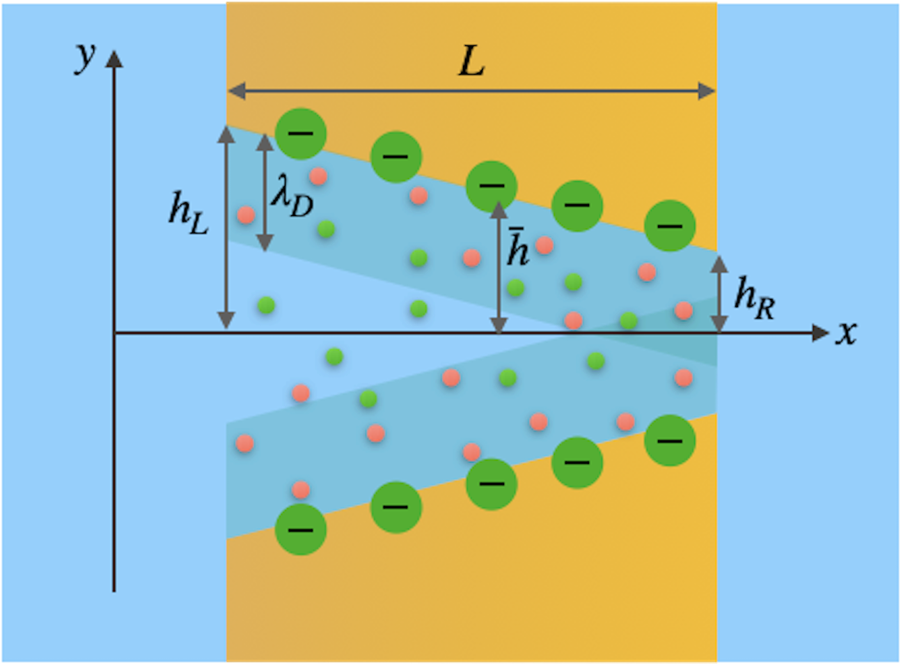
Figure 1: Schematic view of the channel in contact with two reservoirs at fixed salt concentration. The channel width is assumed to be constant along the z direction pointing out of the page. The channel walls carry a uniform negative charge density and a electrically charged double layer forms over a characteristic length $\lambda_{D}$.

The channel is filled with a symmetric monovalent electrolyte composed of species having equal diffusion coefficient $D$, in contact with two reservoirs at fixed temperature $T$ and ionic strength $c_{s}$. Each wall bears a uniform negative surface charge of density $\sigma<0$. We assume $L_{z}\gg\bar{h}$ so that we can neglect the $z$ dependence of any variables of the model and the resulting system is effectively 2D.
In order to characterize the ionic dynamics we derive effective one-dimensional transport equations for the ionic concentration profiles $c_{\pm}$. The approach relies on the constraint of a small aspect ratio $\epsilon=\bar{h}/L\ll 1$ , i.e. a slowly-varying channel geometry. In this case, the transversal relaxation dynamics with characteristic relaxation time $\tau_{y}\sim\bar{h}^{2}/D$ is decoupled from the longitudinal relaxation dynamics with $\tau_{x}\sim L^{2}/D$ and the ions are assumed to instantaneously adjust to the Boltzmann distribution at each cross-section. Such separation of scale is known in the literature as local thermodynamic equilibrium dr Groot and Mazir (1962) (LTE).
Under these assumptions the steady-state Nernst-Planck equation for the positive and negative ionic species reads:

$$j_{\pm}=\mp De\beta c_{\pm}(x,y)\partial_{x}\Phi(x,y)-D\partial_{x}c_{\pm}(x,y)$$ (5)

where $j_{\pm}$ is the constant mass flux density along $x$, $\beta=1/k_{B}T$ and $\Phi(x,y)$ is the total electrostatic potential inside the channel. We have neglected in (5) the advective flux which proved to be minor compared to the electrophoretic contribution for moderate surface charge densities and moderate external fields Ai et al. (2010).
Eq. (5) must be supplemented by the Poisson equation relating the electrostatic potential to the spatial charge distribution $q=e(c_{+}-c_{-})$ inside the channel:

$$\nabla^{2}\Phi(x,y)=-\frac{q(x,y)}{\epsilon_{o}\epsilon_{w}}$$ (6)

In the next section we reduce (5) to an effective 1D equation by introducing the FJ ansatz for the ionic concentration profiles as explained in II.1. For consistency, the same approximation is applied to the Poisson equation together with the assumption of small transversal variation of $\Phi$ (see section II.2), which allows to formally integrate (6).

II.1 The Fick-Jacobs approach

Since the ionic transversal and longitudinal dynamics are assumed to be decoupled, it is convenient to introduce the marginal concentration as the cross-sectional integral of the volumetric concentration:

$$c_{\pm}(x)=\int_{-h(x)}^{+h(x)}dy\ c_{\pm}(x,y)$$ (7)

Moreover, following the approach of Zwanzig Zwanzig (1992) we define $x-$dependent free energies $A_{\pm}(x)$ via:

$$e^{-\beta A_{\pm}(x)}=\frac{1}{\bar{h}}\int_{-h(x)}^{+h(x)}dy\ e^{\mp\beta e\Phi(x,y)}$$ (8)

From the hypothesis of LTE we may factor the volumetric concentrations $c_{\pm}(x,y)$ into the product of equilibrium normalized conditional densities $\xi_{\pm}(y;x)$ and the marginal concentrations,

$$c_{\pm}(x,y)\approx\xi_{\pm}(y;x)\cdot c_{\pm}(x)=\frac{e^{\mp\beta e\Phi(x,y)}}{\displaystyle\int_{-h(x)}^{+h(x)}dy\ e^{\mp\beta e\Phi(x,y)}}\cdot c_{\pm}(x).$$ (9)

Eq. (9) represents the key ansatz of the FJ approach. Martens et al Martens et al. (2011) proved that (9) can be recovered as the zero-order term of a perturbative expansion in series for the geometrical parameter $k$ around the zero-transversal-flux solution. Notably for the case of a conical channel, where $|d_{x}h(x)|=\rm const$, taking into account the extra $x-$dependence of the diffusivity $D(x)$ amounts to a rescaling of the diffusion coefficient thus making the theory here developed valid up to $k\leq 1$ Berezhkovskii, Dagdug, and Bezrukov (2015, 2017).
In the present work we examine the zero-order FJ approximation and we leave to future work the discussion of higher order corrections.

By integrating Eq. (5) in the $y$ coordinate and using (9) as a closure for $c_{\pm}(x,y)$, an effective one-dimensional equation is obtained,

$$J_{\pm}=Dc_{\pm}(x)\left[\frac{\partial_{x}\int_{-h(x)}^{+h(x)}e^{\mp\beta e\Phi(x,y)}dy}{\int_{-h(x)}^{+h(x)}e^{\mp\beta e\Phi(x,y)}dy}\right]-D\partial_{x}c_{\pm}(x)$$ (10)

where $J_{\pm}=\int dy\ j_{\pm}$ is the longitudinal mass flux per unit width for each species. In Eq. (10) the concentrations $c_{\pm}(x)$ are the marginal ones; in the following, we refer to the marginal concentrations unless the both $x-$ and $y-$dependences are explicitly noted.
Now we introduce dimensionless variables. As reported in table 1 we rescale the $x$ coordinate by the total length of the channel $L$ and the coordinate $y$ as well as the Debye length $\lambda_{D}$ and the channel profile $h(x)$ by the half-height $\bar{h}$. In this way the channel profile reads

$$h(x)=1+\frac{\kappa}{2}-\kappa x,$$ (11)

where we also introduced a rescaled channel slope $\kappa=k/\epsilon$. Since we keep fixed the half height $\bar{h}$ allowing for variation in the degree of corrugation we note that $\kappa<2$ for geometrical consistency.
The electrostatic potential is rescaled by the thermal one $k_{B}T/e$ and the volumetric concentrations $c_{\pm}$ by the concentration in the bulk $c_{s}$. Consequently, the charge density $q$ is rescaled by $ec_{s}$, the mass flux $J$ per unit width by $Dc_{s}\bar{h}/L$ and the conductance per unit width, $G=\partial I/\partial\Delta V$ with $I$ the total ionic current and $\Delta V$ the applied potential drop, by the bulk conductance $Dc_{s}\bar{h}e^{2}/k_{B}TL$.
In dimensionless form Eq. (10) now reads:

$$J_{\pm}=-c_{\pm}\Big{[}\partial_{x}\beta A_{\pm}+\partial_{x}\log c_{\pm}\Big{]}=-c_{\pm}\partial_{x}\mu_{\pm}$$ (12)

where we have introduced the (dimensionless) electrochemical potential $\mu_{\pm}=\log c_{\pm}+\beta A_{\pm}$. In Eq. (12) the electrophoretic contribution now appears in terms of the previously introduced effective free energies $A_{\pm}(x)$ . For a neutral species the effective free energy reduces to the standard Boltzmann entropy $\beta A(x)=-\log 2h(x)$. In this case $\frac{d}{dx}\beta A(x)$ is referred to as an entropic force, originating from the variation in phase-space volume available for free diffusion along the channel. For a charged species $A$ embeds both enthalpic and entropic contributions.

Table 1: Adimensionalization of the independent and derived quantities of the model.

Variables	Rescaled variables
Longitudinal coordinate x	x/L
Transversal coordinate y	y/$\bar{h}$
Channel profile h(x)	h(x)/$\bar{h}$
Debye length $\lambda_{D}$	$\lambda_{D}$/$\bar{h}$
Channel slope $\kappa$	k/$\epsilon$
Electrostatic potential $\phi$	$e\phi/k_{B}T$
Volumetric concentrations $c_{\pm}$	$c_{\pm}$/$c_{s}$
Charge density $q$	$q$/$ec_{s}$
Mass fluxes $J_{\pm}$	$J_{\pm}$/$(Dc_{s}\bar{h}$/$L)$
Differential conductance $G$	$G$/$(Dc_{s}\bar{h}e^{2}$/$Lk_{B}T)$

Eq. (12) must be integrated with the appropriate boundary conditions, i.e. by imposing continuity in the electrochemical potential at the ends of the channel .
The discontinuity in the surface charge distribution at the channel ends, and the consequent readjustment of ions within the diffusive layer results in an apparent local discontinuity in the concentration and electrostatic potential profiles. In the present framework, such discontinuities are treated as point-like discontinuities, which stands for the fact that these entrance effects are $\mathit{O}(\epsilon)$, hence they fall within the level of our approximation.

II.2 Local Debye-Hückel approximation

In dimensionless units, the Poisson equation (6) reads

$$\epsilon^{2}\partial_{x}^{2}\Phi+\partial_{y}^{2}\Phi=-\lambda_{D}^{-2}q.$$ (13)

It is convenient to decompose the electrostatic potential as

$$\Phi(x,y)=\psi(x,y)+\langle\phi\rangle(x)+\phi_{ext}(x)$$ (14)

where $\langle\phi\rangle=\frac{1}{2h(x)}\int_{-h(x)}^{+h(x)}dy\ \phi(x,y)$ is the average potential across $y$, $\psi=\phi-\langle\phi\rangle$ in the excess potential at each section and $\phi_{ext}=-\Delta V\left(x-\frac{1}{2}\right)$ is the potential drop applied externally, resulting in a constant electric field directed in the $x$ direction.
By using FJ approximation into Eq. (13) together with (14) and by linearizing in $\psi$ under the assumption of small potential variation in the transversal direction, we reduce (13) to

$$\epsilon^{2}\partial_{x}^{2}\Phi+\partial_{y}^{2}\psi=-\frac{\lambda_{D}^{-2}}{2h}\left[(c_{+}-c_{-})-(c_{+}+c_{-})\psi\right].$$ (15)

We refer to the linearization used to derive Eq. (15) as a local Debye-Huckel (DH) approximation: the potential is linearized with respect to the local cross-sectional average preserving therefore global nonlinearity. We stress that the assumption of small $\psi$ is more general than standard DH, which requires small $\zeta$ potential everywhere (typically Andelman (1995) $\zeta\leq 25mV$). In fact it allows to explore the ideal gas regime for arbitrarily high Dukhin number, where typically the global Debye-Hückel assumption would fail.
The small aspect ratio constraint allows for a lubrication-like approximation of (15) which reduces to a linear equation for $\psi$:

$$\partial_{y}^{2}\psi=-\frac{\lambda_{D}^{-2}}{2h}\left[(c_{+}-c_{-})-(c_{+}+c_{-})\psi\right]$$ (16)

Consistently, the scaling argument applies as well to the electrostatic wall boundary condition, which after neglecting terms of $\mathcal{O}(k^{2})$, and introducing rescaled variables, reduces to

$$\partial_{y}\phi\Big{|}_{y=\pm h}=\mp\frac{Du\ }{\lambda_{D}^{2}}.$$ (17)

We shall note here that the LTE hypothesis previously introduced implies local electroneutrality, in which the integrated charge density balances the surface charge density at each cross-section,

$$\int dy\ q(x,y)=c_{+}(x)-c_{-}(x)=2\ Du.$$ (18)

In fact, by integrating Eq. (15) in the $y-$coordinate, using (17) and neglecting $\mathcal{O}(\epsilon^{2})$ terms, Eq. (18) is obtained.
To first order approximation the FJ ansatz, the lubrication approximation and local electroneutrality are different naming for the same unique assumption, i.e. separation of transversal and longitudinal scales, applied to different physical propertiesMacGillivray (1968). The reduced Poisson equation can be formally integrated leading to

$$\psi=-\frac{Du(x)}{\lambda_{D}(x)}\frac{\cosh(y/\lambda_{D}(x))}{\sinh(h(x)/\lambda_{D}(x))}+\frac{c_{+}(x)-c_{-}(x)}{c_{+}(x)+c_{-}(x)}.$$ (19)

In Eq. (19) the potential is naturally expressed in terms of a local Dukhin number and a local Debye length respectively defined as:

$$\lambda_{D}(x)=\frac{\lambda_{D}}{\sqrt{c_{vol}(x)}}$$ (20)

$$Du(x)=\frac{Du}{c_{vol}(x)}$$ (21)

in terms of the total average volumetric concentration $c_{vol}(x)=[c_{+}(x)+c_{-}(x)]/2h(x)$.
We recognize the first term on the rhs of Eq. (19) to be the Debye-Huckel potential carrying an extra $x-$dependence due to the varying channel geometry. The second term on the rhs ensures local electroneutrality.
Eqs. (12) and (16) need to be solved numerically. It is convenient to rewrite Eq. (12) in terms of $\psi$ :

$$J_{+} = -\partial_{x}c_{+}+c_{+}[\partial_{x}\log h-(\partial_{x}\langle\phi\rangle-\Delta V)+\partial_{x}\log\langle e^{-\psi}\rangle]$$ (22a)

$$J_{-} = -\partial_{x}c_{-}+c_{-}[\partial_{x}\log h+(\partial_{x}\langle\phi\rangle-\Delta V)+\partial_{x}\log\langle e^{+\psi}\rangle]$$ (22b)

$$\partial_{y}^{2}\psi = -\frac{\lambda_{D}^{-2}}{2h}[(c_{+}-c_{-})-(c_{+}+c_{-})\psi]$$ (22c)

so that the coupling between the concentration profiles and the electrostatic potential is made now explicit. We use finite-element simulations (COMSOL) to solve the system of Eqs. (22a)(22b)(22c) in order to look at the electric current $I=J_{+}-J_{-}$ generated by the applied potential drop $\Delta V$. (See appendix for details on the numerical simulations).
The expression for the electric current obtained by formally integrating Eq. (22a) and (22b) reads

$$I=-\frac{1}{2}\left[\frac{e^{-\Delta V/2}-e^{+\Delta V/2}}{\displaystyle\int_{0}^{1}dx^{\prime}\ e^{\beta A_{+}(x^{\prime})}}-\frac{e^{+\Delta V/2}-e^{-\Delta V/2}}{\displaystyle\int_{0}^{1}dx^{\prime}\ e^{\beta A_{-}(x^{\prime})}}\right],$$ (23)

where the denominator is responsible for the non-linear (rectified) response of the channel, as it expresses the coupling between the dissipative dynamics (thermodynamic forcing) and the geometric asymmetry. For a flat channel, Eq. (23) reduces to the standard ohmic responseSchoch, Han, and Renaud (2008) (per unit width) which in dimensional unit reads

$$I_{ohm}=\frac{De^{2}}{k_{B}T}\left[\frac{2c_{-}}{L}+\frac{2\sigma}{eL}\right]\ \Delta V.$$ (24)

Eq. (23) is valid for slowly varying channels under the assumption of small potential variation in the transversal direction. Hence it represents a well-grounded expression for the ionic current allowing to span across different regimes in the electrostatic phase space in both $\lambda_{D}$ and $Du$.
Previously proposed analytical approaches Woermann (2003); Kosińska et al. (2008); Cervera et al. (2006) assume that $\lambda_{D}$ is the relevant controlling parameter by treating separately the case of no overlap $\lambda_{D}\ll 1$ and strong overlap $\lambda_{D}\gg 1$. This is not necessary in the present framework, where $\lambda_{D}$ can vary continuously. Nevertheless, it is useful at this stage to introduce the regime of strong Debye overlap as it represents a well-known scenario which we will use as a benchmark to compare with numerical results.

II.3 Strong Debye overlap, $\lambda_{D}\gg 1$

Let us consider the regime in which the channel height is much smaller than the Debye length. The EDL extends all throughout the interior of the confined electrolyte, rendering the channel perfectly charge-selective. Both the electrostatic potential, $\Phi(x)$, and the ionic concentration profiles, $c_{\pm}(x)$, are assumed to be uniform in the transversal direction allowing for a substantial simplification of the mathematical problem at hand. We stress that the concentrations $c_{\pm}(x)$ here are not the marginal concentrations but the total concentrations which in this limit are independent of $y$.
Together with local electroneutrality which in this case reads

$$2h(x)\left[c_{+}(x)-c_{-}(x)\right]=2Du,$$ (25)

continuity in the chemical potential provides an expression for the Donnan potential at either end of the channel Picallo et al. (2013); Schoch, Han, and Renaud (2008); Constantin and Siwy (2007),

$$\phi_{L}=\frac{1}{2}\log\left[\frac{-Du+\sqrt{Du^{2}+h_{L}^{2}}}{+Du+\sqrt{Du^{2}+h_{L}^{2}}}\right]+\frac{\Delta V}{2},$$ (26a)

$$\phi_{R}=\frac{1}{2}\log\left[\frac{-Du+\sqrt{Du^{2}+h_{R}^{2}}}{+Du+\sqrt{Du^{2}+h_{R}^{2}}}\right]-\frac{\Delta V}{2}.$$ (26b)

Notably, already at equilibrium the varying geometry results in a non-uniform tilted potential across the channel.
Analogously, the channel’s junctions concentrations read

$$c_{L}=c_{L}^{+}+c_{L}^{-}=\frac{\sqrt{Du^{2}+h_{L}^{2}}}{h_{L}},$$ (27a)

$$c_{R}=c_{R}^{+}+c_{R}^{-}=\frac{\sqrt{Du^{2}+h_{R}^{2}}}{h_{R}}.$$ (27b)

Hence, a jump in concentration profiles builds up at each junction of the channel to compensate for the potential discontinuity (26). Such a local balance is known in the literature as local Donnan equilibrium. These expressions will allow for asymptotic analytical predictions for the conductances when $\Delta V\to\pm\infty$.
The equation of motion (12) for $\lambda_{D}\gg 1$ reduces to

$$2h(x)\left[\mp c_{\pm}(x)d_{x}\phi(x)-d_{x}c_{\pm}(x)\right]=J_{\pm},$$ (28)

which, rewritten in terms of the total mass flux $J=J_{+}+J_{-}$ and electric current $I$, becomes

$$J = -2h(x)d_{x}c(x)-2Du\ d_{x}\phi,$$ (29a)

$$I = -2h(x)c(x)d_{x}\phi+2Du\ d_{x}\log 2h(x).$$ (29b)

In (29a-29b) local electroneutrality (25) has been used to further simplify the expressions.

III RESULTS

III.1 Current response and limiting conductances

We focus first on the current response obtained by numerically solving the system (22a-22c) under an applied potential difference $\Delta V$. The two reservoirs are kept at the same ionic strength so that the only thermodynamic force at play is a constant electric field along the longitudinal coordinate. A positive (negative) $\Delta V$ corresponds respectively to the anode being placed at the left (right) reservoir.
A standard measure of ionic rectification is given by the current-voltage (I-V) curve which we report in Fig. (2) for the case of $\lambda_{D}=1/2$ and $Du=1/2$ and for different values of the channel slope. This regime corresponds to the case of partial Debye overlap inside the channel. For instance, in the case of $k=3/2$ the local ratio $\frac{\lambda_{D}}{h(x)}$ spans from $\sim 0.3$ at the base junction up to $\sim 2$ at the tip junction. Therefore by moving from left to right ions experience the building up of a Donnan potential passing from a region (left) where the bulk dominates to a region (right) where the EDL dominates.

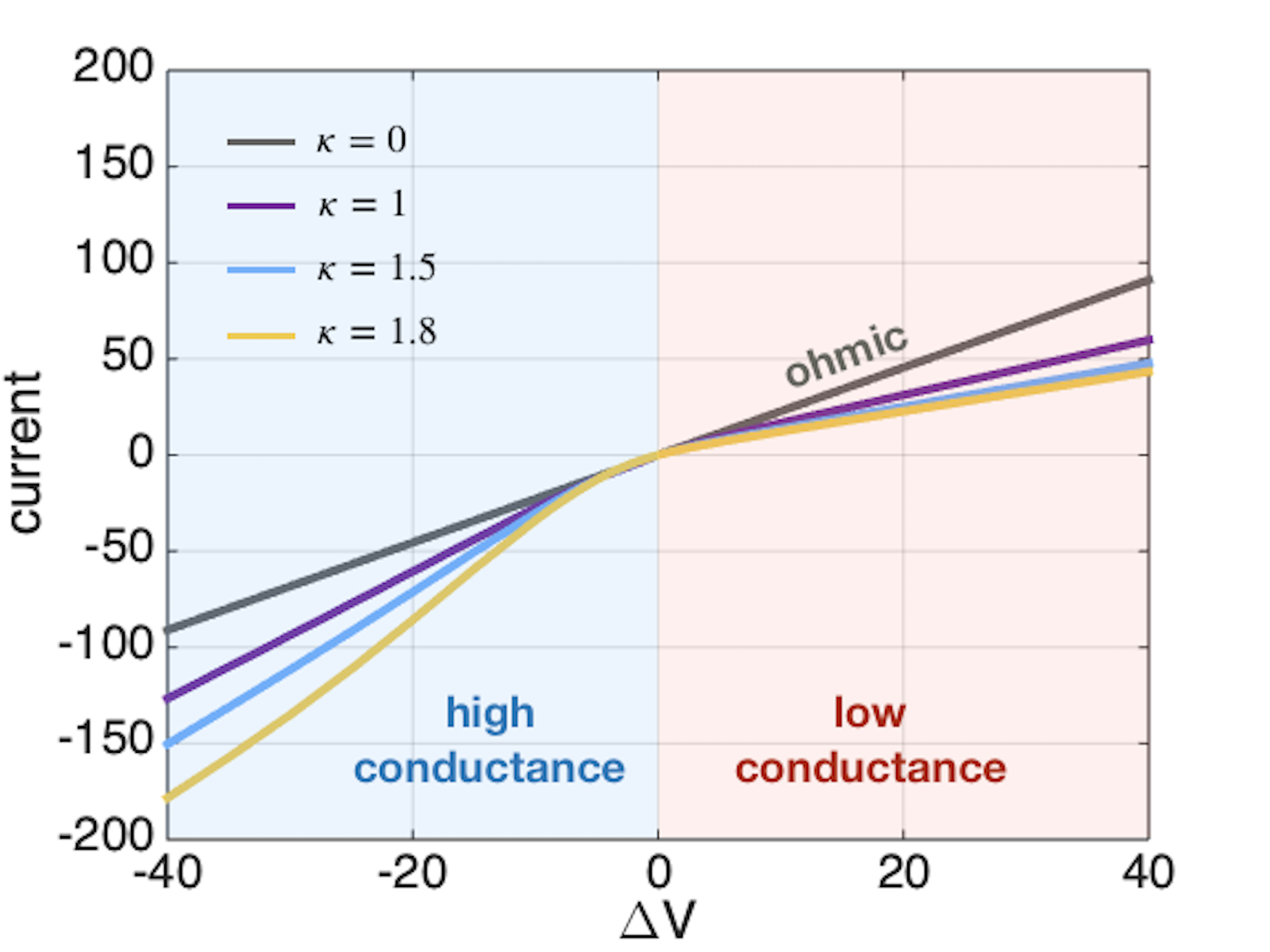
Figure 2: Dimensionless current I as a function of $\Delta V$ for a channel with $\lambda_{D}=1/2$, $Du=1/2$ at different value of channel slope, respectively $\kappa=0,1,3/2,1.8$. We recognize two different conductance states. For positive voltage drop (positive electric field) the system is in a low conductance state, the current being smaller than the Ohmic one (grey line). On the contrary for negative voltage drop (negative electric field) the current is magnified and the system is said to be in a high conductance state.

The non-linear curves in Fig. (2) display the usual diode-like behaviour reported in the literature, with a preferential direction of ionic current. When the electric field is applied parallel to the $x-$direction with the counterions moving from base to tip, the current is suppressed with respect to the Ohmic response (grey curve) and the system is said to be in a low conductance state. On the contrary, when the electric field is applied antiparallel with respect to $x$ with the counterions moving from tip to base, the current is magnified and the system is said to be in a high conductance state.
The rectification magnitude is monotonous in the degree of asymmetry in the system. The greater the channel’s slope the larger the rectification. This must come as no surprise since the channel slope is the only element introducing asymmetry in the system. For $k\to 0$ the channel is flat and it behaves like a standard Ohmic resistor.
The numerical I-V curves can be compared with analytical predictions of the limiting differential conductances

$$G_{\pm\infty}=\lim_{\Delta V\to\pm\infty}\frac{\partial I}{\partial\Delta V}.$$ (30)

For strong Debye overlap the equations of motion reduce to (29a-29b). By neglecting the diffusive contribution to the mass flow with respect to the electrophoretic contribution in (29a) and by integrating in $x$ we obtain

$$J=2Du\Delta V.$$ (31)

Combining Eqs. (29a) and (29b) we solve for $d_{x}c$ in terms of the ratio $\frac{I}{J}$

$$2hd_{x}c+\frac{(2Du)^{2}}{2hc}d_{x}\log 2h=\left(\frac{2Du}{2hc}\frac{I}{J}-1\right)J,$$ (32)

which is bound asymptotically, $\Delta V\to\pm\infty$, if the prefactor on the rhs vanishes, i.e. $\frac{2Du}{2hc}\frac{I}{J}\to 1$. Accordingly the limiting conductance, $G_{\pm\infty}$, reduces to

$$G_{\pm\infty}=\lim_{\Delta V\to\infty}(c_{+}+c_{-}),$$ (33)

because the diffusive contribution to the ionic flux for very large fields is negligible. Eq. (33) implies that the marginal concentration inside the channel approaches a uniform value in the limit $\Delta V\to\pm\infty$. When $\lambda_{D}\gg 1$ we have analytical expressions for the marginal concentration at the channel’s ends where, due to the channel geometry, the left end is characterized by the higher marginal concentration while the right end fixes the lower value. Hence, from Eqs. (27b-27b) (see Discussion section for further details)

$$G_{+\infty}=c_{vol}^{R}=2\sqrt{Du^{2}+h_{R}^{2}},$$ (34a)

$$G_{-\infty}=c_{vol}^{L}=2\sqrt{Du^{2}+h_{L}^{2}}.$$ (34b)

In Fig. (3) we show the I-V curves for $\lambda_{D}=2$ and $Du=1$, i.e. in the regime of strong overlap. For $k=3/2$ we report the analytical predictions for the asymptotic curves $I_{\pm\infty}=\pm G_{\pm\infty}\Delta V$ with the limiting conductances obtained from (34), showing that these analytical expressions accurately capture the numerical results. Further discussion on the saturation mechanism for the conductance are reported in the Discussion section.

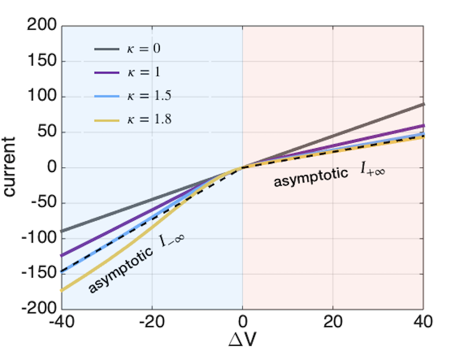
Figure 3: Dimensionless current $I$ as a function of $\Delta V$ for a channel with $\lambda_{D}=2$, $Du=1/2$ at different value of channel slope, respectively $\kappa=0,1,1.5,1.8$. The black dashed lines are the limiting currents for $k=3/2$ in the limit of $\Delta V\to\pm\infty$ using Eqs. (34).

From the comparison between Fig. (2) and Fig. (3) we observe that the quantitative structure of the I-V curves does not change respectively for partial Debye overlap with $\lambda_{D}=1/2$ and strong overlap with $\lambda_{D}=2$. It follows that the Debye length seems not to play a primary role in governing rectification. Notably, this is at odd with previous understanding of ICR which relies on $\lambda_{D}$ as the main controlling parameter.
In the next session this observation is further explored and clarified by looking closely to the dependence of ICR on the electrostatic lengthscales.

III.2 Current rectification ratio

In order to gain further insights on the rectified behaviour of the present system we introduce the rectification ratio $\eta$

$$\eta=\frac{|I(-\Delta V)|}{|I(+\Delta V)|},$$ (35)

defined as the ratio between the absolute value of the current for opposite polarity of the external field. In the case of an ohmic resistor $\eta=1$.
Fig. (4) displays $\eta$ as a function of the external forcing, $\Delta V$, for $\lambda_{D}=1/2$ and $\lambda_{D}=2$. Each plot shows the rectification ratio for different value of the channel slope. The asymptotic predictions for $\eta$ obtained from Eqs. (34a) and (34b) are reported in Fig.(4-b) (dashed black lines).

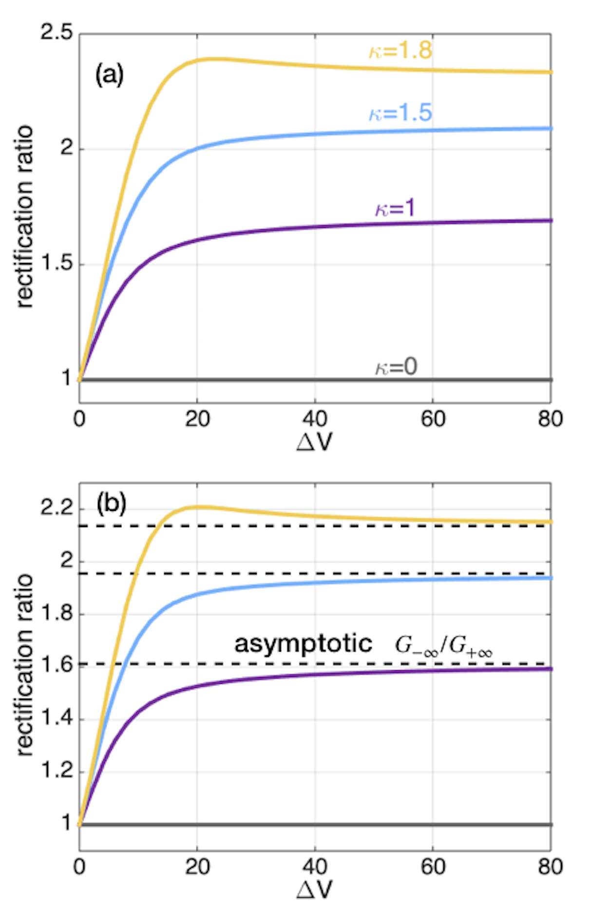
Figure 4: (a) The rectification ratio $\eta$ as a function of the amplitude $|\Delta V|$ in the case of $\lambda_{D}=1/2$ and $Du=1$ for $\kappa=0$, $\kappa=1$, $\kappa=3/2$ and $\kappa=1.8$. For a flat channel $\eta=1$ and the response is linear (gray line). (b) The rectification ratio $\eta$ as a function of the amplitude $|\Delta V|$ in the case of $\lambda_{D}=2$ and $Du=1$ for $\kappa=0$, $\kappa=1$, $\kappa=3/2$ and $\kappa=1.8$. The dashed black lines show the asymptotic value for $\eta$ in the limit of $|\Delta V|\to\infty$.

Fig. (4) shows a saturation behaviour for large value of $\Delta V$. The saturation value increases with the channel slope as already observed for the I-V curves. Moreover for strong overlap the analytical expressions (dashed lines) are in good agreement with the numerical results.
We now turn our attention to the dependence of ICR on the Dukhin number. Fig (5) shows $\eta$ as a function of the reference Dukhin number, Eq. (3), for $\lambda_{D}=2$ and $\kappa=3/2$ for different values of the external forcing. Interestingly, $\eta$ shows a strongly non-monotonic dependence on $Du$ with a maximum of rectification approximately at $Du\approx 1/2$. For $Du\ll 1$ or $Du\gg 1$ the rectification ratio goes to one and the standard ohmic behaviour is recovered. For values of $Du$ close to unity the rectification ratio reaches a maximum which depends on the strength of the applied field upon reaching a saturation value as shown in Fig. (4). The saturation value of $\Delta V$ is itself modulated by $Du$. Fig. (5) shows that $Du$ is a critical parameter controlling rectification, in contrast with $\lambda_{D}$ that seems not to be an adequate parameter to describe ICR. This is further illustrated by looking at Fig. (6), where $\eta$ is plotted as a function of $\lambda_{D}$ for three different values of $Du$. We report a dashed line when we enter the regime in which linearization in $\psi$ is no further justified. This happens in the limit of small $\lambda_{D}$ when the potential at the centerline vanishes and $\psi\sim\zeta$. In the regime of partial and strong overlap no significant dependence on $\lambda_{D}$ is shown. Albeit not quantitative, our results suggest that ICR decreases while approaching the limit of vanishing $\lambda_{D}$. In this limit it is known that ICR approaches a non-zero asymptotic valuePoggioli, Siria, and Bocquet (2019).

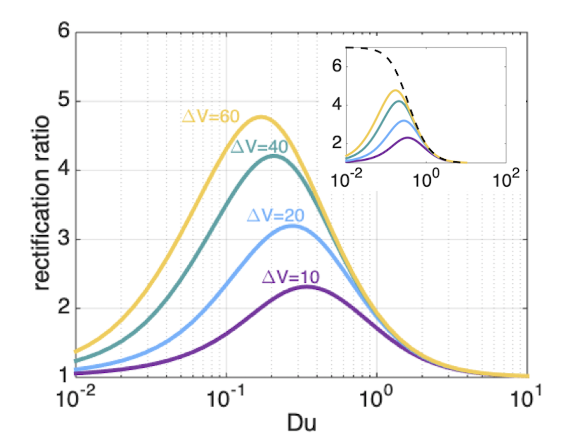
Figure 5: The rectification ratio $\eta$ as a function of the reference $Du$ for a channel with $\lambda_{D}=2$ and $k=3/2$ at different value of external forcing, respectively $\Delta V=10,20,40,60$. In the inset graph the analytical prediction for $\eta$ in the regime of strong overlap and of $|\Delta V|\to\infty$ is reported. For sufficiently large $Du$ it accurately estimates the behaviour of $\eta$ while in the limit of $Du\to 0$ it deviates from the numerical curves because of the breakdown of the hypothesis of strong overlap.

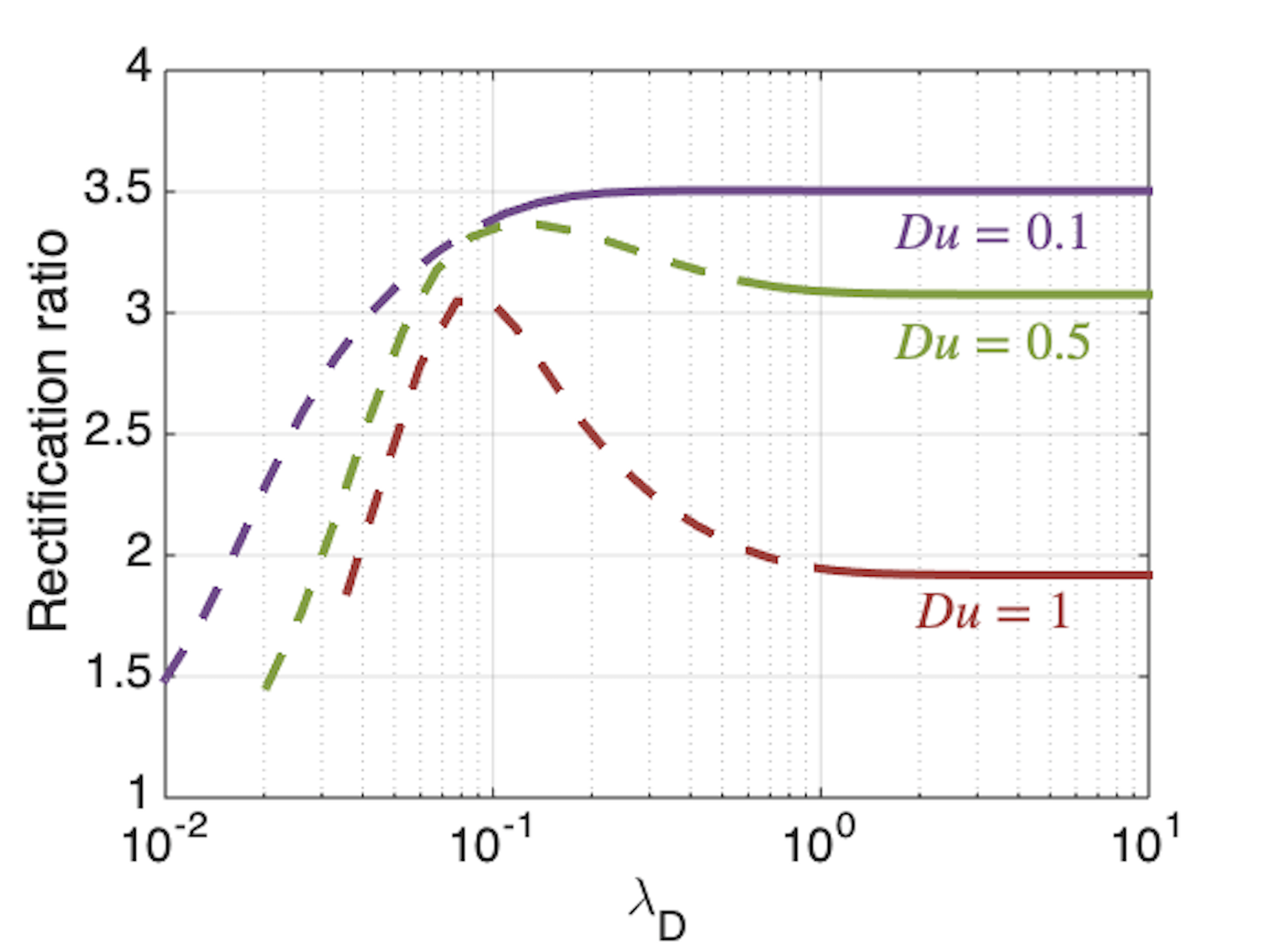
Figure 6: The rectification ratio $\eta$ as a function of the Debye length for different value of the Dukhin, respectively $Du=1/10$, $Du=1/2$, $Du=1$. The channel slope is $\kappa=3/2$ and the potential drop $\Delta V=40$. Dashed lines refer to the regime in which the approximation of local Debye-Hückel approximation is no longer justified.

IV DISCUSSION: The role of Dukhin number

IThe results of the previous section show that ICR is not primarily governed by the Debye length but rather by the Dunkhin length. This suggests that the Dukhin number directly controls the high (low) conductance state, for negative (positive) potential drop.

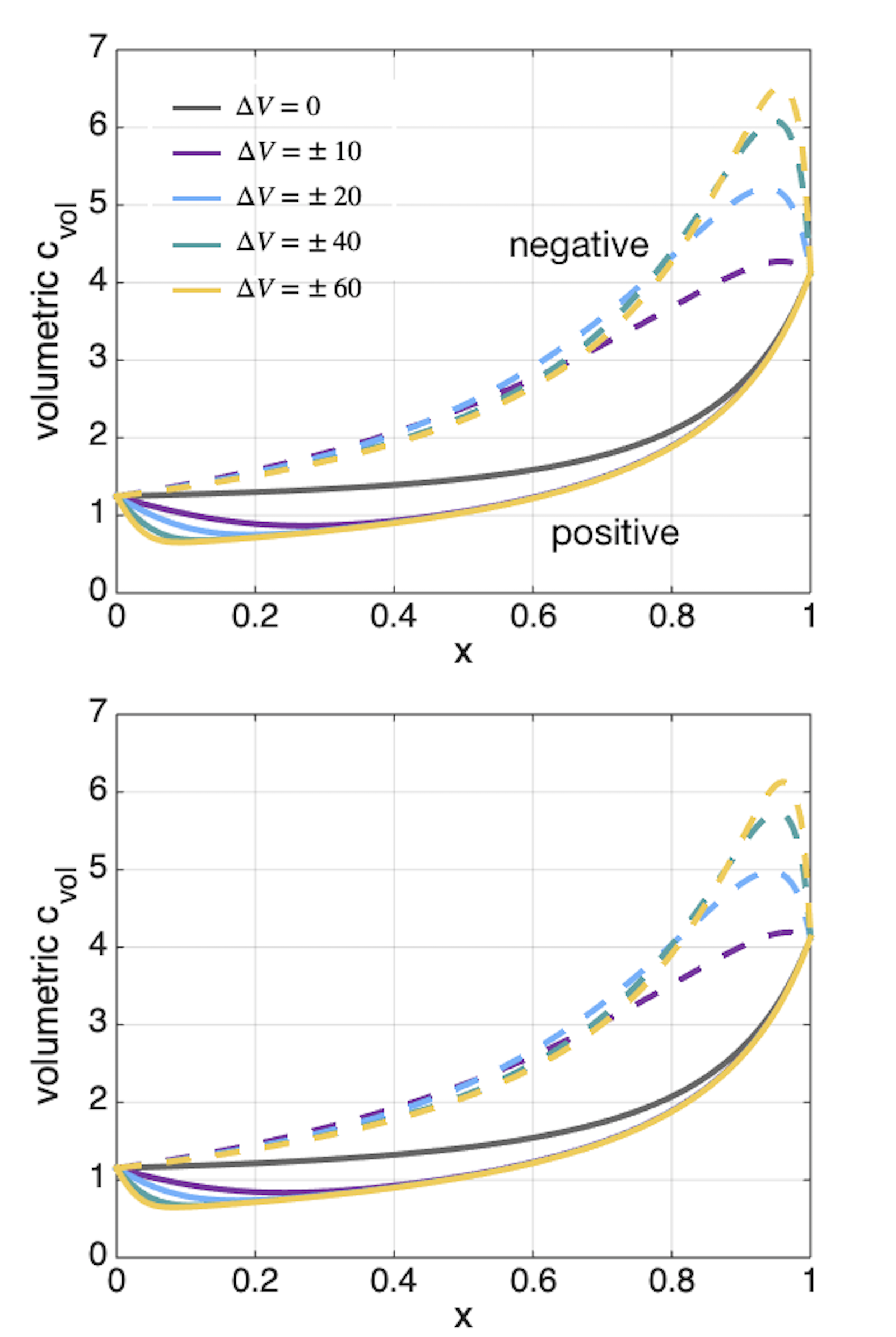
Figure 7: Volumetric cross-section average concentration $c_{vol}$ along the channel axis for different amplitude of the applied potential, respectively $\Delta V=0$, $\Delta V=|10|$, $\Delta V=|20|$, $\Delta V=|40|$ and $\Delta V=|60|$. In the figures solid lines corresponds to a positive potential drop while dashed lines to a negative potential drop. Concentration profiles for the following choice of parameters: (a) $\lambda_{D}=1/2$, $Du=1$ and $\kappa=3/2$ (b) $\lambda_{D}=2$, $Du=1$ and $\kappa=3/2$.

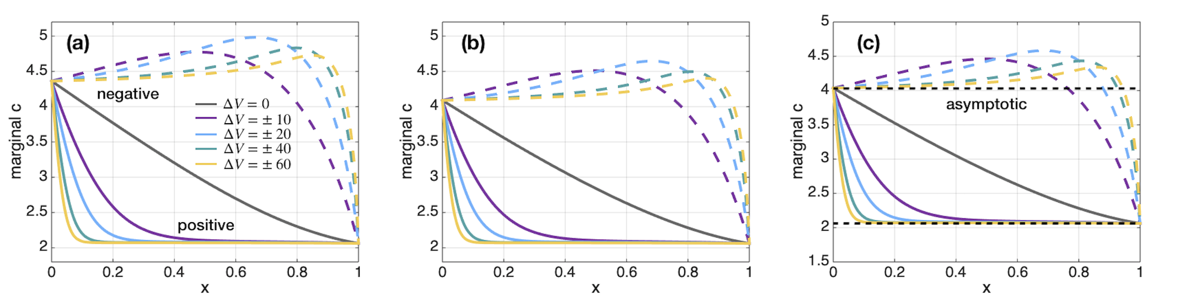
Figure 8: Marginal concentration $c$ along the channel axis for different amplitude of the applied potential, respectively $\Delta V=0$, $\Delta V=|10|$, $\Delta V=|20|$, $\Delta V=|40|$ and $\Delta V=|60|$. In the figures solid lines corresponds to a positive potential drop while dashed lines to a negative potential drop. Concentration profiles for the following choice of parameters: (a) $\lambda_{D}=1/2$, $Du=1$ and $\kappa=3/2$. (b) $\lambda_{D}=1$, $Du=1$ and $\kappa=3/2$ (c) $\lambda_{D}=2$, $Du=1$ and $\kappa=3/2$. The black dashed lines in (c) corresponds to the boundary value for the marginal concentration due to the local Donnan equilibrium (34a) and (34b).

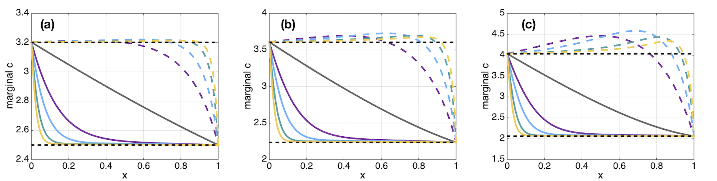
Figure 9: Marginal concentration $c$ along the channel axis for different amplitude of the applied potential, respectively $\Delta V=0$, $\Delta V=|10|$, $\Delta V=|20|$, $\Delta V=|40|$ and $\Delta V=|60|$. In the figures solid lines corresponds to a positive potential drop while dashed lines to a negative potential drop. Concentration profiles for the following choice of parameters: (a) $\lambda_{D}=2$, $Du=1$ and $\kappa=1/2$. (b) $\lambda_{D}=2$, $Du=1$ and $\kappa=1$ (c) $\lambda_{D}=2$, $Du=1$ and $\kappa=3/2$. The black dashed lines corresponds to the boundary value for the marginal concentration due to the local Donnan equilibrium (34a) and (34b).

This can be understood in terms of ionic concentration enrichment and depletion for opposite polarity of the external field, as discussed in previous works Woermann (2003); Siwy (2006); Cervera et al. (2006). The panel in Fig. (7) shows the volumetric cross-sectionally averaged concentration $c_{vol}$ along the channel axis for two different regimes of $\lambda_{D}$ . In both figures we observe an overall increase (decrease) of ionic concentration for negative (positive) $\Delta V$ with respect to the equilibrium profile, represented by the grey line. Therefore the high conductance state for negative $\Delta V$ is due to an increase in ionic concentration inside the channel. The larger the external forcing, the stronger the accumulation of ions. On the contrary, when a positive voltage drop is applied the electrical conductance decreases due to the decrease of ionic concentration.
In order to understand the phenomenon of salt accumulation and depletion we now turn our attention to the behaviour of the marginal concentration for large fields. In the previous section we already anticipated that in the limit of very large potential drop we expect the marginal concentration to saturate to a uniform value along the channel axis. Fig. (8) reports the marginal concentration along the longitudinal axis for increasing value of $\lambda_{D}$ ((a)-(c)). For increasing amplitude of the external forcing the marginal concentration indeed tends to a constant value which is determined by the boundary value at either end of the channel. In the case of a negative potential drop the marginal concentration saturates to the larger boundary value which is the value at the left end of the channel (base). On the other hand, for positive potential drop the saturation value is bounded to the boundary condition at the right site (tip).
Fig. (8) also shows an overshoot in the marginal concentration for large (but finite) negative $\Delta V$. The overshoot is not present in the case of positive $\Delta V$ which stands as an additional sign of the asymmetry in the system. The microscopic mechanism causing it is still not clear and requires further investigations. Fig. (9) reports the marginal concentration profiles for increasing slope of the channel showing a significant dependence of the overshot on $\kappa$.

Fig. (8)(c) displays the marginal concentrations for strong overlap, $\lambda_{D}\gg 1$. Local Donnan equilibrium builds up at the nanopore ends, controlling the corresponding marginal concentrations

$$c_{L}=2h_{L}\sqrt{\left(\frac{Du}{h_{L}}\right)^{2}+1},$$ (36a)

$$c_{R}=2h_{R}\sqrt{\left(\frac{Du}{h_{R}}\right)^{2}+1}.$$ (36b)

Asymptotically, $Du\gg 1$, $c_{L}\to c_{R}$, i.e. $\eta\to 1$. In this regime transport is controlled by the diode surface, where entropic interactions are negligible with respect to electrostatic interactions and ions do not feel the symmetry breaking originated from the confinement. That is to say, enthalpy wins.
The local marginal selectivity, $\gamma_{\pm}(x)$ (directly proportional to the ionic marginal concentrations), constitutes a second, relevant quantity. For the counterions, the local selectivity at either end of the channel respectively reads

$$\gamma_{+}^{L}=\frac{c_{+}^{L}}{(c_{+}^{L}+c_{-}^{L})}=\frac{\frac{Du}{h_{L}}+\sqrt{\left(\frac{Du}{h_{L}}\right)^{2}+1}}{2\sqrt{\left(\frac{Du}{h_{L}}\right)^{2}+1}}$$ (37a)

$$\gamma_{+}^{R}=\frac{c_{+}^{R}}{(c_{+}^{R}+c_{-}^{R})}=\frac{\frac{Du}{h_{R}}+\sqrt{\left(\frac{Du}{h_{R}}\right)^{2}+1}}{2\sqrt{\left(\frac{Du}{h_{R}}\right)^{2}+1}}$$ (37b)

making transparent the key role of the Dukhin number in controlling the local channel selectivity. Eq. (37) quantifies the relative importance of the counterion flux over the total transport. Due to the conical shape of the channel, $\gamma_{+}^{R}$ is larger than $\gamma_{-}^{L}$, meaning that counterion transfer in presence of an external driving is larger at the tip than at the base. Such imbalance in selectivities results in a transient ion readjustment when an external driving is switched on. In the case of counterions moving from tip to base (negative $\Delta V$) this imbalance in selectivities results in a transient accumulation of ions inside the channel. On the contrary, when counterions move from base to tip (positive $\Delta V$) there will be a relative larger amount of ions leaving than entering the channel resulting in an overall decrease of salt concentration. In either case, the stationary state is reached when the nonequilibrium accumulation/depletion dynamics counterbalances the asymmetry of local selectivity induced by the geometry. Eq. (37) implies that the imbalance in selectivities is controlled by the asymmetry between $Du/h_{L}$ and $Du/h_{R}$. Both $Du\ll 1$ and $Du\gg 1$ result in a uniform selectivity between the two ends of the channel, i.e. no rectification (see Fig. (10)). High Dukhin number, $Du\gg 1$, means that the selectivity of counterions at either end tends to one (that is the selectivity of coions tends to zero): the coions are completely excluded from the system and the geometrical asymmetry is nullified by the perfect selectivity of the channel. No bulk transport is present so that the entirety of transport takes place in the EDL. On the other side, for $Du\ll 1$ the selectivity at either ends tends to its bulk value $1/2$. In this regime, irrespectively of the physical extension of the EDL the entirely of transport takes place in the unselective bulk and the omhic bulk response is restored.
The asymmetry between $Du^{L}/h_{L}$ and $Du^{R}/h_{R}$ is maximized for $Du\sim 1$ (in our case $Du\sim 1/2$ because of the normalization used for the marginal concentrations).
The qualitative interpretation of ICR caused by an asymmetry in the local selectivity at either end of the nanochannel is qualitatively consistent with the pioneer proposal of Woarmann Woermann (2003). However, our analysis provides a fresh interpretation of an old puzzle. We have shown that $Du$ is the principal electrostatic parameter that locally controls the channel selectivity, with a secondary effect due to $\lambda_{D}$, while Woermann pointed at $\lambda_{D}$ as the main length to be compared with channel confinement. Although it may fly against intuition, it is not the physical size of the EDL that determines the system capability to rectify ionic current.

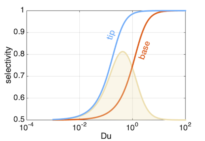
Figure 10: The counterion selectivity at the tip $\gamma_{+}^{R}$(blu) and at the base $\gamma_{+}^{L}$(red) of a channel with $k=3/2$ as a function of the reference Dukhin number. For $Du\sim 1/2$ the difference between the two selectivities (yellow curve) is maximized, leading to a maximum of rectification.

V Conclusion

In summary, we have presented here a theoretical analysis to address the phenomenon of ionic current rectification in nanometric channels. We have specifically focused on the case of a geometric ionic diode where the symmetry breaking is caused only by the conical geometry of the system. The theoretical framework mainly relies on two assumptions: a slowly varying channel geometry and a small electrostatic potential variation in the transversal direction. These ingredients allow us to derive formal expressions for the electrostatic potential, Eq. (19), and for the ionic current, Eq. (23), and to explore the response of the system for different values of $\lambda_{D}$ and $Du$. The main outcome of the work is the identification of the Dukhin length as the primary electrostatic length scale controlling rectification. It follows that rectification is expected to be measured in systems with size comparable to the Dukhin length, which remarkably can reach the micrometer scale Bocquet and Charlaix (2010). This fact may explain recent experimental worksHe et al. (2017); Lin, Yeh, and Siwy (2018) in which ICR is observed in mesoscopic pores.
To conclude by misquoting Wolfrang Pauli , it is a dynamical usage of surfaces that let the nanofluidic diode succeed where demons don’t.

VI Appendix

Here we report some details of the implementation in COMSOL for the numerical integration of the following equations:

$$J_{+} = -\partial_{x}c_{+}+c_{+}[\partial_{x}\log h-(\partial_{x}\langle\phi\rangle-\Delta V)+\partial_{x}\log\langle e^{-\psi}\rangle]$$

$$J_{-} = -\partial_{x}c_{-}+c_{-}[\partial_{x}\log h+(\partial_{x}\langle\phi\rangle-\Delta V)+\partial_{x}\log\langle e^{+\psi}\rangle]$$

$$\partial_{y}^{2}\psi = -\frac{\lambda_{D}^{-2}}{2h}[(c_{+}-c_{-})-(c_{+}+c_{-})\psi]$$ (38)

First of all let us recall here the appropriate boundary conditions for the system at hands. In both ends of the channel we have to impose continuity in the electrochemical potential for each species. Starting from the left side we write in adimensional variables:

$$\log\frac{1}{2}\pm\frac{\Delta V}{2}=\log c_{\pm}(0)+\beta A_{\pm}(0)$$ (39)

where by definition:

$$e^{-\beta A_{\pm}(0)}=e^{\mp\frac{\Delta V}{2}}\int_{-h_{L}}^{+h_{L}}dy\ e^{\mp\phi(0,y)}$$ (40)

By substituting eq.(40) into (39) we obtain:

$$c_{\pm}(0)=\frac{1}{2}\int_{-h_{L}}^{+h_{L}}dy\ e^{\mp\phi_{L}(y)}$$ (41)

where the boundary condition for $c_{\pm}(0)$ is expressed in terms of the function $\phi_{L}(y)\equiv\phi(0,y)$. The latter is obtained by solving the following transversal equation at $x=0$:

$$\partial_{y}^{2}\phi_{L}=-\frac{\lambda_{D}^{2}}{2+\kappa}\left[\int_{-h_{L}}^{+h_{L}}\sinh(\phi_{L})-(\phi_{L}-\langle\phi_{L}\rangle)\int_{-h_{L}}^{+h_{L}}\cosh(\phi_{L})\right],\hskip 28.45274pt{x=0}$$ (42)

where $\langle\phi_{L}\rangle=\frac{1}{2h_{L}}\int_{0}^{h_{L}}dy\phi_{L}(y)$ , $h_{L}=1+\frac{\kappa}{2}$ and we made use of the fact that:

$$c_{+}(0)+c_{-}(0)=\int_{-h_{L}}^{+h_{L}}dy\cosh(\phi_{L}(y))$$

$$c_{+}(0)-c_{-}(0)=\int_{-h_{L}}^{+h_{L}}dy\sinh(\phi_{L}(y))$$ (43)

Eq. (42) can be then numerically integrated using the standard electrostatic boundary conditions:

$$\partial_{y}\phi_{L}(0) = 0$$

$$\partial_{y}\phi_{L}(\pm h_{L}) = \mp\frac{Du}{\lambda_{D}^{2}}$$ (44)

Likewise we find the appropriate boundary value for $c_{\pm}(1)$ using :

$$c_{\pm}(1)=\frac{1}{2}\int_{-h_{R}}^{+h_{R}}dy\ e^{\mp\phi_{R}}$$ (45)

Therefore the expressions (41) and (45) are now numbers which can be directly used as boundary conditions for the system in (VI).
It is also convenient in COMSOL to rescale the $y$ variable in the following way:

$$y\to h(x)y\prime$$ (46)

$$f(x,y)\to f(x,h(x)y\prime)\equiv f\prime(x,y\prime)$$ (47)

In this way we map the original domain to a square domain substantially simplifying the COMSOL calculation. From the chain rule it follows:

$$\partial_{x}f(x,y)\to\partial_{x}f\prime(x,y\prime) = \partial_{x}f\prime(x,y\prime)+\partial_{y\prime}f\prime(x,y\prime)\partial_{x}y\prime$$ (48a)

$$= \partial_{x}f\prime(x,y\prime)-\partial_{y\prime}f\prime(x,y\prime)\frac{y\prime}{h(x)}d_{x}h(x)$$

$$\partial_{y}f(x,y)\to\partial_{y}f\prime(x,y\prime) = \partial_{y\prime}f\prime(x,y\prime)d_{y}y\prime$$ (48b)

$$= \partial_{y\prime}f\prime(x,y\prime)\frac{1}{h(x)}$$

The only variables in the model that depend on $y$ are $\psi(x,y)$, $\phi_{L}(y)$ and $\phi_{R}(y)$. For each of them we apply (48) so that the electrostatic boundary condition for $\psi$ (likewise for $\phi_{L}$ and $\phi_{R}$) become:

$$\partial_{y\prime}\psi\prime(x,y\prime=0) = 0$$ (49)

$$\partial_{y\prime}\psi\prime(x,y\prime=\pm 1) = \mp\frac{Du}{\lambda_{D}^{2}}h(x)$$ (50)

and the rescaled Poisson equation:

$$\partial^{2}_{y\prime}\psi\prime=-\frac{\lambda_{D}^{-2}}{2}h(x)\left[(c_{+}-c_{-})-\psi\prime(c_{+}+c_{-})\right]$$ (51)

References

- Cheng and Guo (2010) L.-J. Cheng and L. J. Guo, “Nanofluidic diodes,” Chem. Soc. Rev. 39, 923–938 (2010).
- Siwy and Fuliński (2002) Z. Siwy and A. Fuliński, “Fabrication of a synthetic nanopore ion pump,” Phys. Rev. Lett. 89, 198103 (2002).
- Siwy et al. (2005) Z. Siwy, I. D. Kosińska, A. Fuliński, and C. R. Martin, “Asymmetric diffusion through synthetic nanopores,” Phys. Rev. Lett. 94, 048102 (2005).
- Umehara et al. (2006) S. Umehara, N. Pourmand, C. D. Webb, R. W. Davis, K. Yasuda, and M. Karhanek, “Current rectification with poly-l-lysine-coated quartz nanopipettes,” Nano Letters 6, 2486–2492 (2006), pMID: 17090078, https://doi.org/10.1021/nl061681k .
- Nguyen, Vlassiouk, and Siwy (2010) G. Nguyen, I. Vlassiouk, and Z. S. Siwy, “Comparison of bipolar and unipolar ionic diodes,” Nanotechnology 21, 265301 (2010).
- Laohakunakorn et al. (2015) N. Laohakunakorn, V. V. Thacker, M. Muthukumar, and U. F. Keyser, “Electroosmotic flow reversal outside glass nanopores,” Nano Letters 15, 695–702 (2015), pMID: 25490120, https://doi.org/10.1021/nl504237k .
- Jubin et al. (2018) L. Jubin, A. Poggioli, A. Siria, and L. Bocquet, “Dramatic pressure-sensitive ion conduction in conical nanopores,” Proceedings of the National Academy of Sciences 115, 4063–4068 (2018), http://www.pnas.org/content/115/16/4063.full.pdf .
- Perry et al. (2010) J. M. Perry, K. Zhou, Z. D. Harms, and S. C. Jacobson, “Ion transport in nanofluidic funnels,” ACS Nano 4, 3897–3902 (2010), pMID: 20590127, https://doi.org/10.1021/nn100692z .
- Cheng and Guo (2007) L.-J. Cheng and L. J. Guo, “Rectified ion transport through concentration gradient in homogeneous silica nanochannels,” Nano Letters 7, 3165–3171 (2007), pMID: 17894519, https://doi.org/10.1021/nl071770c .
- Karnik et al. (2007) R. Karnik, C. Duan, K. Castelino, H. Daiguji, and A. Majumdar, “Rectification of ionic current in a nanofluidic diode,” Nano Letters 7, 547–551 (2007), pMID: 17311461, https://doi.org/10.1021/nl062806o .
- Harrell et al. (2006) C. C. Harrell, Y. Choi, L. P. Horne, L. A. Baker, Z. S. Siwy, and C. R. Martin, “Resistive-pulse dna detection with a conical nanopore sensor,” Langmuir 22, 10837–10843 (2006), pMID: 17129068, https://doi.org/10.1021/la061234k .
- Wei et al. (2012) R. Wei, V. Gatterdam, R. Wieneke, R. Tampé, and U. Rant, “Stochastic sensing of proteins with receptor-modified solid-state nanopores,” Nature Nanotechnology 7 (2012).
- Xie et al. (2008) Y. Xie, X. Wang, J. Xue, K. Jin, L. Chen, and Y. Wang, “Electric energy generation in single track-etched nanopores,” Applied Physics Letters 93, 163116 (2008), https://doi.org/10.1063/1.3001590 .
- Siria et al. (2013) A. Siria, P. Poncharal, A.-L. Biance, R. Fulcrand, X. Blase, S. T. Purcell, and L. Bocquet, “Giant osmotic energy conversion measured in a single transmembrane boron nitride nanotube,” Nature 494, 455 EP – (2013).
- Wu, Ramiah Rajasekaran, and Martin (2016) X. Wu, P. Ramiah Rajasekaran, and C. R. Martin, “An alternating current electroosmotic pump based on conical nanopore membranes,” ACS Nano 10, 4637–4643 (2016), pMID: 27046145, https://doi.org/10.1021/acsnano.6b00939 .
- Zhang and Schatz (2017) Y. Zhang and G. C. Schatz, “Conical nanopores for efficient ion pumping and desalination,” The Journal of Physical Chemistry Letters 8, 2842–2848 (2017), pMID: 28590134, https://doi.org/10.1021/acs.jpclett.7b01137 .
- Picallo et al. (2013) C. B. Picallo, S. Gravelle, L. Joly, E. Charlaix, and L. Bocquet, “Nanofluidic osmotic diodes: Theory and molecular dynamics simulations,” Phys. Rev. Lett. 111, 244501 (2013).
- Bocquet and Charlaix (2010) L. Bocquet and E. Charlaix, “Nanofluidics, from bulk to interfaces,” Chem. Soc. Rev. 39, 1073–1095 (2010).
- Sui et al. (2001) H. Sui, B.-G. Han, J. K. Lee, P. Walian, and B. K. Jap, “Structural basis of water-specific transport through the aqp1 water channel,” Nature 414, 872 EP – (2001), article.
- Tsong and Xie (2002) T. Tsong and T. Xie, “Ion pump as molecular ratchet and effects of noise: electric activation of cation pumping by na,k-atpase,” Applied Physics A 75, 345–352 (2002).
- Bhattacharya et al. (2011) S. Bhattacharya, J. Muzard, L. Payet, J. Mathé, U. Bockelmann, A. Aksimentiev, and V. Viasnoff, “Rectification of the current in -hemolysin pore depends on the cation type: The alkali series probed by molecular dynamics simulations and experiments,” The Journal of Physical Chemistry C 115, 4255–4264 (2011), pMID: 21860669, https://doi.org/10.1021/jp111441p .
- Malgaretti, Pagonabarraga, and Rubi (2013) P. Malgaretti, I. Pagonabarraga, and M. Rubi, “Entropic transport in confined media: a challenge for computational studies in biological and soft-matter systems,” Frontiers in Physics 1, 21 (2013).
- Siwy (2006) Z. Siwy, “Ion-current rectification in nanopores and nanotubes with broken symmetry,” Advanced Functional Materials 16, 735–746 (2006), https://onlinelibrary.wiley.com/doi/pdf/10.1002/adfm.200500471 .
- Cheng and Guo (2009) L.-J. Cheng and L. J. Guo, “Ionic current rectification, breakdown, and switching in heterogeneous oxide nanofluidic devices,” ACS Nano 3, 575–584 (2009), https://doi.org/10.1021/nn8007542 .
- He et al. (2017) X. He, K. Zhang, T. Li, Y. Jiang, P. Yu, and L. Mao, “Micrometer-scale ion current rectification at polyelectrolyte brush-modified micropipets,” Journal of the American Chemical Society 139, 1396–1399 (2017), pMID: 28095691, https://doi.org/10.1021/jacs.6b11696 .
- Lin, Yeh, and Siwy (2018) C.-Y. Lin, L.-H. Yeh, and Z. S. Siwy, “Voltage-induced modulation of ionic concentrations and ion current rectification in mesopores with highly charged pore walls,” The Journal of Physical Chemistry Letters 9, 393–398 (2018), pMID: 29303587, https://doi.org/10.1021/acs.jpclett.7b03099 .
- 199 (1995) “3 - electric double layers,” in Solid-Liquid Interfaces, Fundamentals of Interface and Colloid Science, Vol. 2, edited by J. Lyklema (Academic Press, 1995) pp. 3–1 – 3–232.
- Constantin and Siwy (2007) D. m. c. Constantin and Z. S. Siwy, “Poisson-nernst-planck model of ion current rectification through a nanofluidic diode,” Phys. Rev. E 76, 041202 (2007).
- Ai et al. (2010) Y. Ai, M. Zhang, S. W. Joo, M. A. Cheney, and S. Qian, “Effects of electroosmotic flow on ionic current rectification in conical nanopores,” The Journal of Physical Chemistry C 114, 3883–3890 (2010), https://doi.org/10.1021/jp911773m .
- Kubeil and Bund (2011) C. Kubeil and A. Bund, “The role of nanopore geometry for the rectification of ionic currents,” The Journal of Physical Chemistry C 115, 7866–7873 (2011), https://doi.org/10.1021/jp111377h .
- Wang et al. (2014) J. Wang, M. Zhang, J. Zhai, and L. Jiang, “Theoretical simulation of the ion current rectification (icr) in nano-pores based on the poisson–nernst–planck (pnp) model,” Phys. Chem. Chem. Phys. 16, 23–32 (2014).
- Woermann (2003) D. Woermann, “Electrochemical transport properties of a cone-shaped nanopore: high and low electrical conductivity states depending on the sign of an applied electrical potential difference,” Phys. Chem. Chem. Phys. 5, 1853–1858 (2003).
- Martens et al. (2011) S. Martens, G. Schmid, L. Schimansky-Geier, and P. Hänggi, “Entropic particle transport: Higher-order corrections to the fick-jacobs diffusion equation,” Phys. Rev. E 83, 051135 (2011).
- Yang et al. (2017) X. Yang, C. Liu, Y. Li, F. Marchesoni, P. Hänggi, and H. P. Zhang, “Hydrodynamic and entropic effects on colloidal diffusion in corrugated channels,” Proceedings of the National Academy of Sciences 114, 9564–9569 (2017), http://www.pnas.org/content/114/36/9564.full.pdf .
- Marbach, Dean, and Bocquet (2018) S. Marbach, D. S. Dean, and L. Bocquet, “Transport and dispersion across wiggling nanopores,” Nature Physics 14, 1108–1113 (2018).
- Jacobs (1967) M. Jacobs, Diffusion Processes (Springer Berlin Heidelberg, 1967).
- Zwanzig (1992) R. Zwanzig, “Diffusion past an entropy barrier,” The Journal of Physical Chemistry 96, 3926–3930 (1992), https://doi.org/10.1021/j100189a004 .
- Burada et al. (2007) P. S. Burada, G. Schmid, D. Reguera, J. M. Rubí, and P. Hänggi, “Biased diffusion in confined media: Test of the fick-jacobs approximation and validity criteria,” Phys. Rev. E 75, 051111 (2007).
- Berezhkovskii, Dagdug, and Bezrukov (2015) A. M. Berezhkovskii, L. Dagdug, and S. M. Bezrukov, “Range of applicability of modified fick-jacobs equation in two dimensions,” The Journal of Chemical Physics 143, 164102 (2015), https://doi.org/10.1063/1.4934223 .
- Reguera et al. (2006) D. Reguera, G. Schmid, P. S. Burada, J. M. Rubí, P. Reimann, and P. Hänggi, “Entropic transport: Kinetics, scaling, and control mechanisms,” Phys. Rev. Lett. 96, 130603 (2006).
- Secchi et al. (2016) E. Secchi, A. Niguès, L. Jubin, A. Siria, and L. Bocquet, “Scaling behavior for ionic transport and its fluctuations in individual carbon nanotubes,” Phys. Rev. Lett. 116, 154501 (2016).
- Malgaretti, Pagonabarraga, and Rubi (2014) P. Malgaretti, I. Pagonabarraga, and J. M. Rubi, “Entropic electrokinetics: Recirculation, particle separation, and negative mobility,” Phys. Rev. Lett. 113, 128301 (2014).
- Kosińska et al. (2008) I. D. Kosińska, I. Goychuk, M. Kostur, G. Schmid, and P. Hänggi, “Rectification in synthetic conical nanopores: A one-dimensional poisson-nernst-planck model,” Phys. Rev. E 77, 031131 (2008).
- dr Groot and Mazir (1962) S. dr Groot and P. Mazir, Non-equilibrium Thermodynamics (North-Holland Publishing Company, 1962).
- Berezhkovskii, Dagdug, and Bezrukov (2017) A. M. Berezhkovskii, L. Dagdug, and S. M. Bezrukov, “First passage, looping, and direct transition in expanding and narrowing tubes: Effects of the entropy potential,” The Journal of Chemical Physics 147, 134104 (2017), https://doi.org/10.1063/1.4993129 .
- Note (1) From Eq. (12) we see that by imposing a continuous electrochemical potential throughout the system we ensure finite fluxes everywhere.
- Andelman (1995) D. Andelman, “Chapter 12 - electrostatic properties of membranes: The poisson-boltzmann theory,” in Structure and Dynamics of Membranes, Handbook of Biological Physics, Vol. 1, edited by R. Lipowsky and E. Sackmann (North-Holland, 1995) pp. 603 – 642.
- Note (2) The name refers to the fact that in this regime the only contribution to the electrostatic pressure between the two walls come from the entropy of an homogeneous solution of noninteractive ions .
- MacGillivray (1968) A. D. MacGillivray, “Nernst‐planck equations and the electroneutrality and donnan equilibrium assumptions,” The Journal of Chemical Physics 48, 2903–2907 (1968), https://doi.org/10.1063/1.1669549 .
- Schoch, Han, and Renaud (2008) R. B. Schoch, J. Han, and P. Renaud, “Transport phenomena in nanofluidics,” Rev. Mod. Phys. 80, 839–883 (2008).
- Cervera et al. (2006) J. Cervera, B. Schiedt, R. Neumann, S. Mafé, and P. Ramírez, “Ionic conduction, rectification, and selectivity in single conical nanopores,” The Journal of Chemical Physics 124, 104706 (2006), https://doi.org/10.1063/1.2179797 .
- Poggioli, Siria, and Bocquet (2019) A. R. Poggioli, A. Siria, and L. Bocquet, “Beyond the tradeoff: Dynamic selectivity in ionic transport and current rectification,” The Journal of Physical Chemistry B 123, 1171–1185 (2019), https://doi.org/10.1021/acs.jpcb.8b11202 .
- Note (3) As Pauli once said God makes the bulk; the surface was invented by the devil.