Mesoscopic valley filter in graphene Corbino disk containing a p-n junction

Abstract

The Corbino geometry allows one to investigate the propagation of electric current along a p-n interface in ballistic graphene in the absence of edge states appearing for the familiar Hall-bar geometry. Using the transfer matrix in the angular-momentum space we find that for sufficiently strong magnetic fields the current propagates only in one direction, determined by the magnetic field direction and the interface orientation, and the two valleys, K and K’, are equally occupied. Spatially-anisotropic effective mass may suppress one of the valley currents, selected by the external electric field, transforming the system into a mesoscopic version of the valley filter. The filtering mechanism can be fully understood within the effective Dirac theory, without referring to atomic-scale effects which are significant in proposals operating on localized edge states.

I Introduction

One-dimensional conduction channels associated with edge states are often considered as background for solid-state quantum information processing not only in systems showing the quantum Hall effect Ban18 ; Mro18 ; Bee03 ; Wil07 ; Aba07 ; Car11 ; Zim17 ; Can18 , but also in graphene Fuj96 ; Nak96 or transition metal dichalcogenide nanoribbons Col18 . The aforementioned nanostructures are formed of two-dimensional materials that host an additional electronic valley degree of freedom, allowing dynamic control and the developement of valleytronic devices Sch16 , such as the valley filter Ryc07 ; Ryc08 .

The operation of early proposed valley filters in graphene, employing the constriction with zigzag edges Ryc07 or the line defect Gun11 , was strongly affected by atomic-scale defects Akh08 and local magnetic order Wim08a . To overcome these difficulties, alternative proposals utilizing strain-induced pseudomagnetic fields Zha11 ; Jia13 ; Set16 ; Mil16 ; Zha17 ; Zha18 , disorder and curvature effects in carbon nanotubes Pal11 , or various types of domain walls in graphene, bilayer graphene Sch15 , or topological systems Pan15 , were put forward. Despite such theoretical and computational efforts the experimental breakthrough is still missing, although some recent progress can be noticed Gor14 ; Mak14 ; Shi15 . Therefore, conceptually novel mechanisms of valley filtering are very desired.

In this paper, we explore the possibility of valley filtering for peculiar edge states mixing Landau levels from both sides of the p-n interface in the quantum Hall regime Wil07 ; Aba07 ; Car11 . Such unconventional edge states can be regarded as degenerate versions of snake states, recently observed in ultraclean graphene devices Ric15 ; Mak18 (see Fig. 1). As the charge density is centered far from physical edges of the system, and transport is essentially of a mesoscopic, rather than nanoscopic, nature (i.e., the wavefunction varies on a length scale given by the magnetic length $l_{B}=\sqrt{\hbar/eB}\gg{}a$, with $a=0.246\,$nm being the lattice parameter; see Ref. Liu15 ), some of the above-mentioned obstacles in sustaining the valley polarization of current may be overcome. Additionally, the Corbino geometry Ryc10 ; Kat10 ; Pet14 ; Kum18 allows one to elliminate conventional edge states, making it possible to fully control the spatial distribution of electric current via external electric and magnetic fields.

Possible classical carrier trajectories for weak-to-moderate magnetic fields are depicted schematically in top and middle panels of Fig. 1. Snake states (bottom panel) cannot be understood fully clasically, as they involve relativistic Klein tunneling through the region of an opposite polarity. In the quantum Hall regime the current flows along one section of the p-n interface only (see Fig. 2). The physical meaning of a “weak”, “moderate”, or “strong”, field is determined by mutual relatios between the characteristic sample length $L\equiv{}R_{o}-R_{i}$ (with the outer disk radius $R_{o}$ and the inner radius $R_{i}$), the magnetic length $l_{B}$ ($\ \propto{}B^{-1/2}$), and the cyclotron radius $r_{c}$ ($\ \propto{}B^{-1}$) cycradfoo . In turn, the larger the disk size the lower field is required to elliminate currents distant from the p-n interface, providing the sake of scalability missing in previously proposed nanoscopic valley filters claquafoo .

We show, using the numerical transfer-matrix technique, that the presence of a non-uniform staggered potential, introducing the position-dependent mass term in the effective Dirac equation for low-energy excitations Kat12 , leads to a spatial separation of valley currents and that the valley polarization may be controlled by changing the gate potentials (see Fig. 3). Althought to set a staggered potential one needs to initially modify the sample on a microscopic level, e.g., by chemical functionalization Bou09 ; Hab10 ; Hon13 or the adsorption of hexagonal boron nitride (h-BN) Sac11 ; Yan14 , the operation of such a mesoscopic valley filter is then fully-electrostatically controlled. We further find, that the constant magnetic field of $1\,$T is sufficient to obtain a nearly perfect polarization in the disk of a $400\,$nm diameter. What is more, the filter operation can be directly attributed to a peculiar combination of symmetry breakings for the Dirac Hamiltonian: The mass term breaks the effective time-reversal symmetry in a single valley (symplectic symmetry), whereas the magnetic field breaks the true time-reversal symmetry (involving the valley exchange). Together, these two symmetry-breaking factors lead to the inequivalence of valleys, providing an opportunity to produce nonequilibrium valley polarization of current.

The paper is organised as follows: In Sec. II, we briefly present the effective Dirac theory and the transfer matrix approach to the scattering problem in the angular-momentum space (adjusted to the Corbino-disk symmetry). In Sec. III, we discuss our numerical results concernig the current distribution and valley filtering in the presence of external electromagnetic field and the staggered potential. The conclusions are given in Sec. IV.

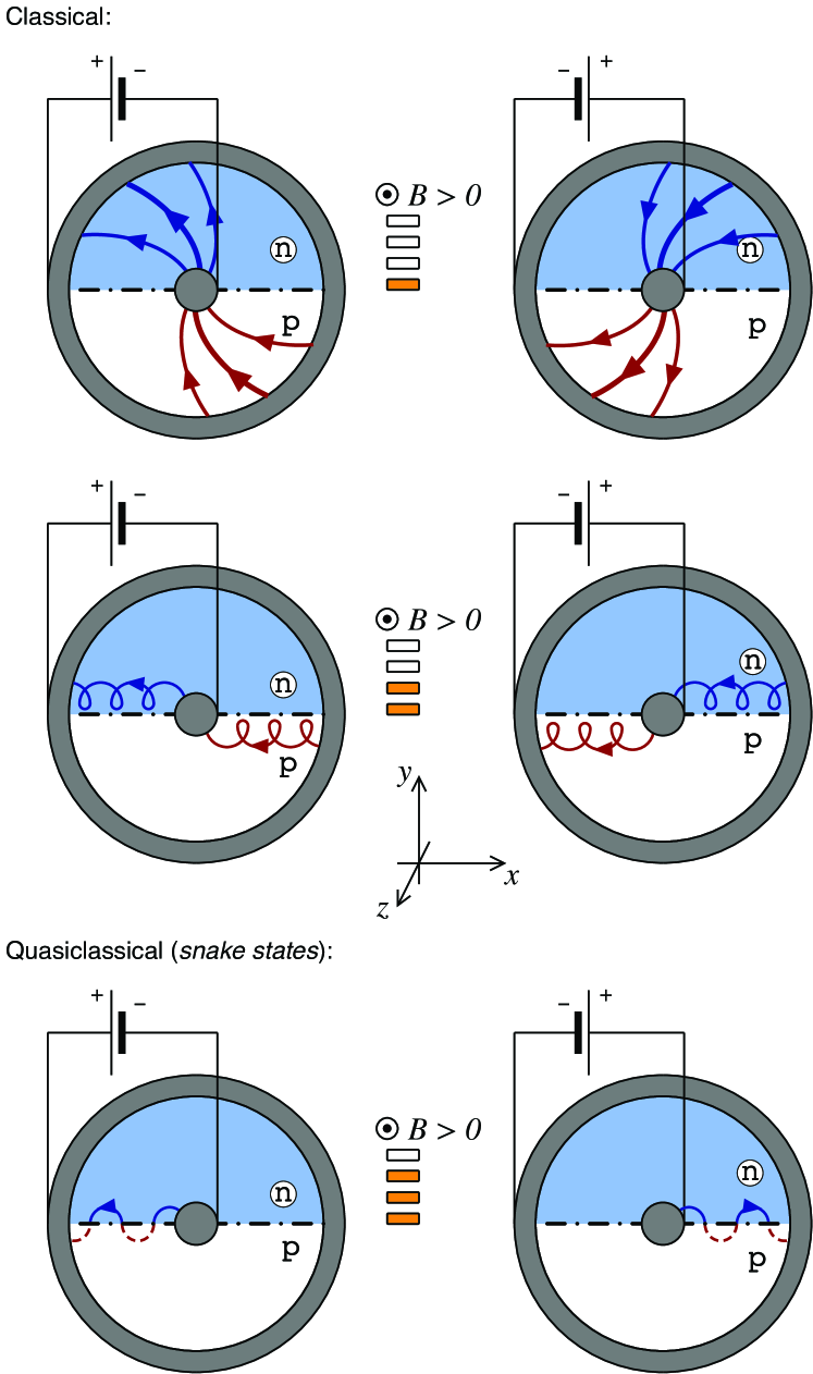
Figure 1: Classical and quasiclassical trajectories (schematic) for electrons (blue lines with arrows) and holes (red lines with arrows) in graphene Corbino disk containing a p-n junction (black dash-dot line) placed in a weak (top panel), moderate (middle panel), and strong (bottom panel) magnetic field ${\mbox{\boldmath$B$}}=(0,0,B)$, with $B>0$. Left and right subplots correspond to the opposite polarity of a voltage source driving a current between circular leads (shadow areas). The coordinate system used in the calculations is also shown.

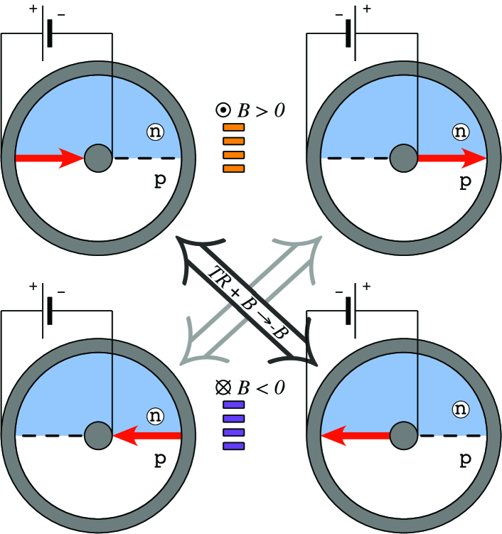
Figure 2: Quantum Hall states propagating along a p-n junction in the strong-field limit, for $B>0$ (top) and $B<0$ (bottom). Diagonal double arrows indicate the system symmetry upon a simultaneous time reversal and magnetic field inversion.

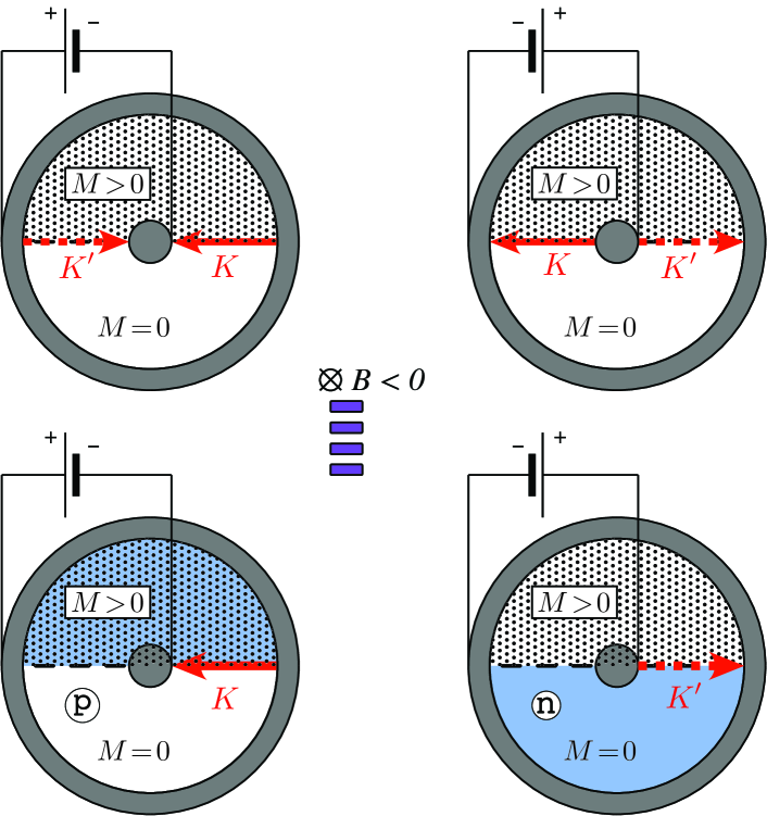
Figure 3: The separation of valley currents (top) and the valley polarization (bottom). A constant staggered potential induces the effective mass $M>0$ in the upper half of the disk (dotted area). Gate electrodes (not shown) tune the doping in the lower half which is undoped (top), $p$-doped (bottom left), or $n$-doped (bottom right).

II Model and methods

II.1 The effective Dirac equation

Let us start by considering a ring-shaped sample, characterized by the inner radius $R_{i}$ and the outer radius $R_{o}$, surrounded by metallic contacts modelled by heavily-doped graphene areas (we set $R_{o}=4R_{i}=200\,$nm for all systems considered in the paper). Since we focus on smooth (or long-range) disorder, the intervalley scattering can be neglected and one can consider the single-valley Dirac equation

$$\left(\xi\pi_{x}\sigma_{x}+\pi_{y}\sigma_{y}\right)\psi\left(r,\phi\right)=\\ \left[E-\mathcal{V}\left(r,\phi\right)-\mathcal{M}\left(r,\phi\right)\sigma_{z}\right]\psi\left(r,\phi\right),\$$ (1)

where $\xi=1$ ($-1$) is the valley index for $K$ ($K^{\prime}$) valley, $\sigma_{\alpha}$ (with $\alpha=x,y,z$) is the Pauli matrix, $\pi_{\alpha}/v_{F}=\left(-i\hbar\partial_{\alpha}+eA_{\alpha}\right)$ is the gauge-invariant momentum operator with $v_{F}\approx 10^{6}\,$m/s the Fermi velocity, $E$ denotes the Fermi energy, and $\mathcal{V}\left(r,\phi\right)$ and $\mathcal{M}\left(r,\phi\right)$ are position-dependent electrostatic potential energy and mass (respectively) in polar coordinates $\left(r,\phi\right)$. We choose the symmetric gauge $\boldsymbol{A}=\frac{B}{2}\left(-y,x\right)$ with a uniform magnetic field $B$. Furthermore, $B\neq 0$ for the disk area ($R_{i}<r<R_{o}$) only; inside the leads ($r<R_{i}$ or $r>R_{o}$) we simply set $B=0$, as the value of $B$ becomes irrelevant in the high-doping limit (see e.g. Ref. Ryc10 ).

In the case of a system with cylindrical symmetry (namely, $\mathcal{V}$ and $\mathcal{M}$ being $\phi$-independent), the Hamiltonian in Eq. (1) commutes with the angular-momentum operator, $L_{z}=-i\hbar\partial_{\phi}+\xi\hbar\sigma_{z}/2$, and the wavefunction can be expressed as a product of radial and angular parts

$$\psi_{l}\left(r,\phi\right)=\varphi_{l}\left(\phi\right)\theta_{l}\left(r\right)\equiv e^{i(l-\xi\sigma_{z}/2)\phi}\left[\begin{array}[]{c}\theta_{A,l}\left(r\right)\\ \theta_{B,l}\left(r\right)\end{array}\right],$$ (2)

where $l$ is an half-odd integer, and $A$ ($B$) labels the upper (lower) spinor element.

II.2 Mode-matching in the angular-momentum space

To solve the scatering problem numerically we simplify here, for the case of a monolayer, the method earlier developed for the Corbino disk in bilayer graphene Rut16 .

If $\mathcal{V}$ or $\mathcal{M}$ in Eq. (1) is $\phi$-dependent the cylindrical symmetry is broken, however, one still can employ the angular-momentum eigenfunctions to represent a general solution as a superposition

$$\psi\left(r,\phi\right)=\sum_{k}\psi_{k}\left(r,\phi\right),$$ (3)

with $\psi_{k}\left(r,\phi\right)$ given by Eq. (2) [see also Appendix A].

Substituting the above into Eq. (1) we obtain

$$\sum\limits_{k}\hbar v_{F}\left[\partial_{r}-f^{k}\left(r\right)\right]\psi_{k}\left(r,\phi\right)=\\ \sum\limits_{k}\xi\left\{i\sigma_{x}\left[E-\mathcal{V}\left(r,\phi\right)\right]-\sigma_{y}\mathcal{M}\left(r,\phi\right)\right\}\psi_{k}\left(r,\phi\right),$$ (4)

where $f^{k}\left(r\right)=\left[\xi\left(k/r+l_{B}^{-2}r/2\right)\sigma_{z}-1/\left(2r\right)\mathbb{I}_{2\times 2}\right]$, the magnetic length $l_{B}=\sqrt{\hbar/\left(eB\right)}$, and $\mathbb{I}_{n\times n}$ is the $n\times n$ identity matrix. Multiplication over the conjugate angular wavefunction $\varphi_{l}^{*}\left(\phi\right)$ and subsequent integration over the polar angle $\phi$ leads to

$$\left[\partial_{r}-f^{l}\left(r\right)-i\sigma_{x}\frac{\xi E}{\hbar v_{F}}\right]\theta_{l}\left(r\right)=\\ \sum_{k}\xi\left[-i\sigma_{x}\mathbb{V}_{lk}\left(r\right)-\sigma_{y}\mathbb{M}_{lk}\left(r\right)\right]\theta_{k}\left(r\right),$$ (5)

with

$$\mathbb{V}_{lk}\left(r\right)=\frac{1}{2\pi}\intop_{0}^{2\pi}d\phi\left[\mathcal{V}\left(r,\phi\right)/\left(\hbar v_{F}\right)\right]e^{i(k-l)\phi},$$ (6)

and

$$\mathbb{M}_{lk}\left(r\right)=\frac{1}{2\pi}\intop_{0}^{2\pi}d\phi\left[\mathcal{M}\left(r,\phi\right)/\left(\hbar v_{F}\right)\right]e^{i(k-l)\phi}.$$ (7)

(Notice that the angular dependence of $\mathcal{V}$ or $\mathcal{M}$ introduces the mode-mixing in our scattering problem.)

The general solution of Eq. (5) can be written as a vector $\boldsymbol{\theta}\left(r\right)=\left[\theta_{l_{min}}^{A}\left(r\right),...,\theta_{l_{max}}^{A}\left(r\right),\theta_{l_{min}}^{B}\left(r\right),...,\theta_{l_{max}}^{B}\left(r\right)\right]^{T}$, with cutoff angular-momentum quantum numbers $l_{min}$ and $l_{max}$. (Hereinafter, $L=l_{max}-l_{min}+1$ is the total number of transmission modes.) Subsequently, one can write

$$\left\{\left[\partial_{r}+1/\left(2r\right)\right]\mbox{$\mathbb{I}$}_{2L\times 2L}-\xi\sigma_{z}\otimes\mathbb{L}\right\}\boldsymbol{\theta}\left(r\right)=\\ \xi\left[i\frac{E}{\hbar v_{F}}\sigma_{x}\otimes\mathbb{I}_{L\times L}-i\sigma_{x}\otimes\mathbb{V}-\sigma_{y}\otimes\mathbb{M}\right]\boldsymbol{\theta}\left(r\right),$$ (8)

where $\mathbb{A}\otimes\mathbb{B}$ is the Kronecker product of matrices $\mathbb{A}$ and $\mathbb{B}$, and the diagonal matrix

$$\mathbb{L}=\mbox{diag}\left(\frac{l_{min}}{r}+\frac{r}{2l_{B}^{2}},\frac{l_{min}\!+\!1}{r}+\frac{r}{2l_{B}^{2}},\right.\\ \left.\dots,\frac{l_{max}}{r}+\frac{r}{2l_{B}^{2}}\right).$$ (9)

Once the scattering matrix is determined (see Appendix A for details), transport properties of the system can be calculated within the Landauer-Büttiker formalism in the linear-response regime Lan70 ; But92 . In particular, the electrical conductance and valley polarization are given by

$$G=G_{0}\sum_{\xi=\pm{}1}\mbox{Tr}\,\mathbf{T}_{\xi},\ \ \ \ \ \ {\cal P}=\frac{\mbox{Tr}\,\mathbf{T}_{\xi=1}-\mbox{Tr}\,\mathbf{T}_{\xi=-1}}{\mbox{Tr}\,\mathbf{T}_{\xi=1}+\mbox{Tr}\,\mathbf{T}_{\xi=-1}},$$ (10)

where $G_{0}=2e^{2}/h$, the prefactor $2$ marks the spin degeneracy (we neglect the Zeeman effect zeemafoo ), and $\mathbf{T}_{\xi}=\mathbf{t}_{\xi}^{\dagger}\mathbf{t}_{\xi}$ with $\mathbf{t}_{\xi}$ being the transmission matrix for one valley. We further neglect the electron-electron interaction and electron-phonon coupling, which is a common approach to nanosystems in monolayer graphene close to the Dirac point, as the scattering processes associated with these many-body effects are usually slower than the ballistic-transport processes Mue09 ; Luc18 .

The matrix $\mathbf{t}$ is also employed when calculating the radial current density, which is given by

$$j_{r}\left(r,\phi\right)=ev_{F}\sum_{l}\psi_{l}^{\dagger}\!\left(r,\phi\right)J_{r}({\phi})\,\psi_{l}\left(r,\phi\right),$$ (11)

with the radial current density operator

$$J_{r}({\phi})=\xi\sigma_{x}\cos\phi+\sigma_{y}\sin\phi,$$ (12)

and $\psi_{l}\left(r,\phi\right)=\sum_{k}\left(\mathbf{t}_{\xi}\right)_{l,k}\,e^{i(k-\xi\sigma_{z}/2)\phi}\left(1,\xi\right)^{T}/\sqrt{r}$ being the transmitted wavefunction in the outer contact ($r>R_{o}$). The matrix element $\left(\mathbf{t}_{\xi}\right)_{l,k}$ denotes the transmission probability amplitude from channel $k$ to $l$. Similarly, the cartesian components of the current density ${\mbox{\boldmath{$j$}}}(r,\phi)=\left(\,j_{x},j_{y}\,\right)$ are calculated by replacing the operator $J_{r}$ in Eq. (11) by

$$J_{x}=\xi\sigma_{x}\ \ \ \ \text{or }\ \ \ \ J_{y}=\sigma_{y}\ \ \ \ \text{(respectively)}.$$ (13)

III Quantum transport in crossed electric and magnetic fields

III.1 Definitions

In order to study a role of the p-n junction in quantum transport through graphene-based Corbino disk, we choose the electrostatic potential energy as follows

$$\mathcal{V}\left(r,\phi\right)=-e\mathcal{E}r\sin\left(\phi-\phi_{V}\right),$$ (14)

where $\mathcal{E}$ is the electric field (we further define $V\equiv{}e\mathcal{E}R_{o}$) and the angle $\phi_{V}$ defines the crystallographic orientation of the p-n interface Luk07 ; Shy09 . Furthermore, we investigate how the transport is affected by the mass term

$$\mathcal{M}\left(r,\phi\right)=M\Theta\left(\phi-\phi_{M}\right)\Theta\left(\pi+\phi_{M}-\phi\right),$$ (15)

with the angle $\phi_{M}$ specifying the mass arrangement, and $\Theta\left(x\right)$ being the Heaviside step function. The mass term given by Eq. (15) is restricted to a half of the disk, $\phi\in\left[\phi_{M},\pi+\phi_{M}\right]$, see Fig. 4. In the heavily-doped contact regions, $\mathcal{V}\left(r,\phi\right)=\mathcal{M}\left(r,\phi\right)=0$.

It is worth to mention that we have also considered other functional forms of the mass term, inluding $\mathcal{M}\left(r,\phi\right)$ smoothly varying with the distance from a p-n junction, always finding a parameter range in which the valley-filtering mechanism that we describe was highly efficient. Even for a simple model given by Eq. (15), changing the Fermi energy ($E$) allows one to shift a p-n interface ($E-\mathcal{V}\left(r,\phi\right)=0$) with respect to the mass boundary, leading to a rich phase diagram discussed later in this section.

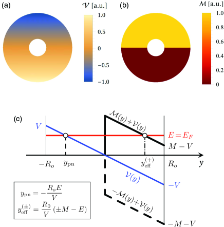
Figure 4: (a) Electrostatic potential energy $\mathcal{V}\left(r,\phi\right)$ given by Eq. (14) with $\phi_{V}=0$, corresponding to a homogeneous electric field $\mathbf{E}=\left(0,\mathcal{E}\right)$. (b) The mass term $\mathcal{M}\left(r,\phi\right)$ given by Eq. (15) with $\phi_{M}=0$ (i.e., $\mathcal{M}=M\neq{}0$ in the upper half of the disk only). (c) Crossections of the electrostatic potential energy ${\cal V}(y)$ (blue line) and the effective potentials ${\cal V}(y)\pm{}{\cal M}(y)$ (black solid or dashed line) along the disk diameter: $x=0$, $-R_{o}\leqslant y\leqslant{}R_{o}$, for some $V,M>0$. Red line marks the Fermi energy $E$. The expressions for $y_{\rm pn}$ (the position of a p-n interface), following from ${\cal V}(y_{\rm pn})=E$, and $y_{\rm eff}^{(\pm)}$ (for which ${\cal V}\pm{\cal M}=E$) are also given. (The inner-lead edges, $y=\pm{}R_{i}$, are omitted for clarity.)

The specific forms of the potential energy $\mathcal{V}\left(r,\phi\right)$ and the mass term $\mathcal{M}\left(r,\phi\right)$, given by Eqs. (14) and (15), lead to the matrix elements

$$\mathbb{V}_{lk}=-\delta_{\left|l-k\right|,1}\frac{Vr\pi}{hv_{F}R_{o}}\,i^{k-l}\exp\left[i\left(k-l\right)\phi_{V}\right],$$ (16)

and

$$\mathbb{M}_{lk}=\frac{Mr}{hv_{F}R_{o}}\begin{cases}\pi&\mbox{\mbox{if $\left|l-k\right|=1$}},\\ i\frac{1-(-1)^{k-l}}{k-l}\mbox{e}^{i\left(k-l\right)\phi_{M}}&\mbox{if $\left|l-k\right|\neq 1$}.\end{cases}$$ (17)

III.2 Quantum Hall regime in the massless case

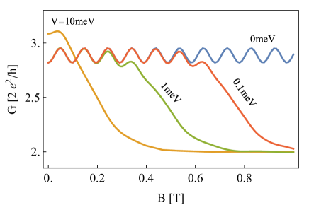
Figure 5: Magnetoconductance of the Corbino disk with $R_{o}=4R_{i}=200\,$nm, $E=M=0$, and different values of the in-plane electric field ${\cal E}$ (quantified by $V\equiv{}e{\cal E}R_{o}$). Notice that the conductance ($G$) approaches the one quantum value ($4e^{2}/h$) for any $V\neq{}0$ at sufficiently high magnetic field ($B$).

We consider now the case of $M=0$ in Eq. (15). The Fermi energy is set as $E=0$ and thus the p-n interface overlaps with the disk diameter ($y_{\rm pn}=0$) for any $V\neq{}0$.

For moderate values of the electric field ($|V|<10\,$meV) and weak magnetic fields the magnetoconductance behavior is same as in a case without the p-n junction Ryc10 , see Fig. 5. The increase of $G$ at weak magnetic fields, visible for $|V|=10\,$meV, indicates the system is close to the ballistic transport regime. This occurs when the (position-dependent) cyclotron diameter $2{}r_{c}(0,y)\gtrsim{}R_{o}\!-\!R_{i}$, enhancing vertical currents along the classical trajectories (cf. the top panel in Fig. 1). For our choice of the parameters, the cyclotron radius,

$$r_{c}(x,y)=\frac{|E-{\cal V}(x,y)|}{eBv_{F}},$$ (18)

is bounded by $r_{c}(0,y)\geqslant{}(R_{i}/R_{o})|V|/\left(eBv_{F}\right)$ along the vertical diameter ($x=0$) and for $R_{i}\leqslant{}|y|\leqslant{}R_{o}$.

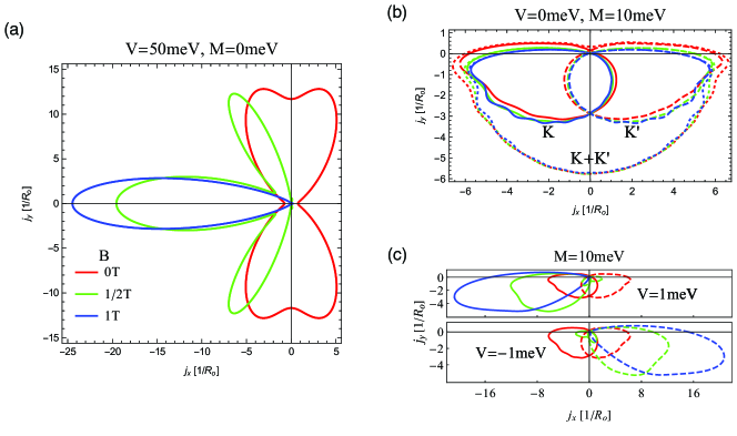
Figure 6: Parametric plots of the current density $\left.\mbox{\boldmath$j$}(r,\phi)\right|_{r=R_{o}}\equiv{}(j_{x},j_{y})$ [see Eq. (13)], where $0\leqslant{}\phi<2\pi$, for the same setup as in Fig. 5 with the electrostatic potential and mass magnitudes ($V$ and $M$) varied between the subplots. Line colours (same for each subplot) mark different magnetic fields: $B=0$ (red), $B=1/2\,$T (green), and $B=1\,$T (blue). (a) For $M=0$, the results are identical for both valleys. A relatively large value of $V=50\,$meV elliminates the pseudodiffusive charge-transport regime. At $1\,$T field, the distribution resembles the analytical result for an infinite plane with the p-n junction, see Fig. 11 in Appendix B. (b) For $V=0$ and $M=10\,$meV, the separation of valley currents appears. Solid and dashed lines correspond to distinct contributions from the two valleys ($K$, $K^{\prime}$); dotted lines depict the current density summarized over the valleys ($K+K^{\prime}$). (c) For $M=10\,$meV and $V=\pm{}1$meV (top/bottom panel), polarity of the p-n junction allows one to select one of the valley currents and suppress the other. (The summarized current density is omitted for clarity.)

Another apparent feature of the data presented in Fig. 5 is a rapid conductance drop, occuring for any $V\neq{}0$ at sufficiently high field. Unlike in a uniformely-doped disk out of the charge-neutrality point, where $G$ vanishes in the high-field limit Ryc10 , here $G$ approaches the value of $4e^{2}/h$ (i.e., the conductance quantum with spin and valley degeneracies) signalling the crossover from pseudodiffusive to quantum-hall transport regime. The limiting value of $G$ reproduces the experimental result of Ref. Pet14 , and can be easily explained by analysing symmetries of the Dirac theory Bee08 .

A bit more detailed view of the effect is provided with the evolution of angle-dependent current density at the outer disk edge ($r=R_{o}$) with increasing field, presented in Fig. 6(a). We choose a high electric field ($V=50\,$meV) to ensure the system undergoes a crossover directly from ballistic to quantum-Hall transport regime, as the contribution from evenescent waves is negligible. For $B=0$ (red line) the current flows in directions along which the doping is extremal, namely, $\phi=\pm{}\pi/2$. For higher fields the transport is dominated by a single direction, for which $\mathcal{V}\left(r,\phi\right)=0$ (i.e., $\phi=\pi$), with some secondary currents at $|\phi|\lesssim\pi/2$ visible for $B=1/2\,$T (green line), and vanising for $B=1\,$T (blue line). This picture is in agreement with the results of previous theoretical studies (see Ref. Bee08 and Appendix B for details).

As the magnetic length at $1$ Tesla field $l_{B}(B\!=\!1\,\text{T})\approx{}26\,$nm is still comparable with the system size (in particular, the inner radii $R_{i}=50\,$nm), the transport cannot be understood classically or quasiclasically. Therefore, several features depicted schematically in Fig. 1 (such as the orbits in the middle panel) have no correspondants in numerical results presented in Fig. 6(a). However, an apparent asymmetry of the current distribution for $B\neq{}0$ is directly linked to the left-right mirror symmetry breaking, also present in the classical level: Both the trajectories and quantum-hall edge states are symmetric upon a simulaneous left-right reflection and the field inversion (cf. Fig. 2); the same applies to the voltage-source polarity (or time) reversal combined with the magnetic field inversion.

III.3 Mass term and the valley filter operation

So far, we have put $M=0$ in Eq. (15) and the transport characteristics were identical for both valleys (K and K’). A different picture emerges in the system with nonzero and spatially-varying mass term (the $M\neq{}0$ case). Our simplified model, in which the mass is present only in the upper half of the system (see Fig. 4), already allows to demonstrate the mesoscopic valley-filtering mechanism. In this subsection, we present the central results of the paper, providing a quantitative description of the effects depicted schematically in Fig. 3.

Quite surprisingly, even at zero electric and magnetic fields the currents corresponding to different valleys are well separated (see Fig. 6(b)). This can be interpreted as a zero-doping version the edge-state formation (the Fermi energy is fixed at $E=0$). As the mass opens a band gap in the upper half of the disk ($0<\phi<\pi$), there are no extended states available, and the current is pushed away towards the lower half ($-\pi<\phi<0$). In turn, the border between areas with ${\cal M}=0$ and ${\cal M}\neq{}0$ plays a role of an artificial edge of the system (notice that the p-n junction is absent for $V=0$). The total current distribution (dotted lines in Fig. 6(b)) is approximately uniform in the lower half of the disk (as this part is in the pseudodiffusive charge-transport regime), with some local maxima for $\phi\approx{}0$ and $\phi\approx{}-\pi$, signaling contributions from the zero-energy edge states. The emergence of such states is well-described in graphene literature, see e.g. Ref. Wim09 ; their analogs in bilayer graphene in a position-dependent perpendicular electric field were also discussed Sch15 . A basic reasoning why electrons in different valleys prefer opposite directions of propagation is given in Appendix C.

A direct link between the valley polarization of current and the direction of propagation for zero-energy edge states leads to the spatial separation of valley currents, which is apparent even in our relatively small system, for which the role of evenescent waves is still significant (and manifests itself by a nonozero current density for any $-\pi<\phi<0$).

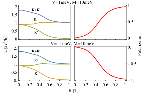
Figure 7: Conductance (left) and valley polarization (right) defined by Eq. (10) for the Corbino disk with both the mass term and the p-n interface displayed as functions of the magnetic field. Remaining system parameters are same as in Fig. 6(c).

Next, the valley-filtering mechanism is demonstrated by creating the p-n interface in a presence of the mass term ($V\neq{}0$, $M\neq{}0$). Fig. 6(c) shows a strong suppression of one of the valley currents in relatively weak electric and magnetic fields (and the valley is selected by a sign of $V$), provided that the mass term is sufficently strong. The valey polarization ${\cal P}$ gradually increases with the magnetic field, becoming almost perfect for $B=1\,$T (see Fig. 7).

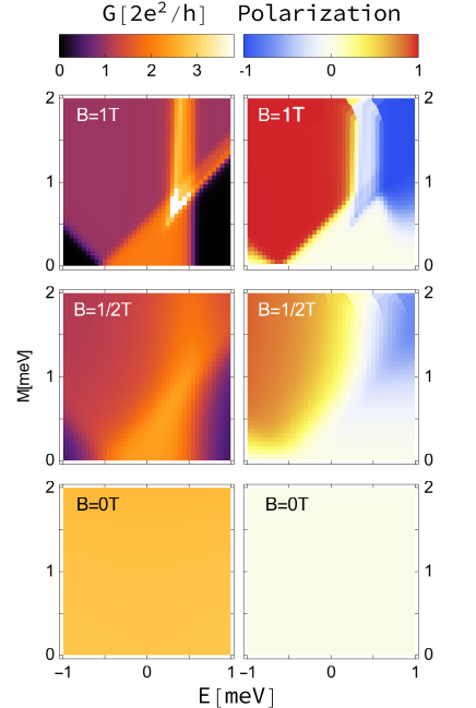
Figure 8: Conductance (left) and valley polarization (right) for $V=1\,$meV as functions of the Fermi energy ($E$) and the mass term ($M$). The value of magnetic field ($B$) is varied between the panels. Remaining system parameters are same as in Fig. 5.

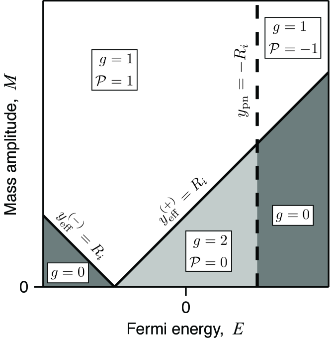
Figure 9: Sketch of the high-field “phase diagram” for some $V>0$ (see top panel in Fig. 8) with distinct regions characterized by dimensionless conductance $g=G/G_{0}$ and the polarization ${\cal P}$, with the boundaries given by mutual relation between the Fermi energy and the potentials ($\,{\cal V}\!\pm{}\!{\cal M}$ and ${\cal V}\,$) at the inner disk edge: $y_{\rm eff}^{(\pm)}=R_{i}$ (solid lines) and $y_{\rm pn}=-R_{i}$ (dashed line). [See also Fig. 4(c).]

The operation of our valley filter is characterized in details by the numerical results presented in Fig. 8, where we have fixed $V=1\,$meV, and visualized the transport characteristics in the Fermi energy-mass ($E$–$M$) parameter plane, for three selected values of the magnetic field ($B=0$, $1/2$, and $1\,$T). Notice that varying $E$ corresponds to a vertical shift of the p-n interface; in particular, for $E=VR_{i}/R_{o}=0.25\,$meV we have $y_{\rm pn}=-R_{i}$ (cf. Fig. 4) and the p-n interface is a tangent line to the inner disk edge at the lower (i.e., mass-free) half. At zero magnetic field, the density maps shown in bottom panels are perfectly uniform, and no valley polarization is visible. For higher fields, distinct regions of the "phase diagram" are formed, including the unpolarized highly-conducting region ($G\approx{}2G_{0}$, ${\cal P}\approx{}0$) at the central-bottom part of each subplot, the two polarized highly-conducting regions ($G\approx{}G_{0}$, ${\cal P}\approx{}\pm{}1$) near the upper corners, and the two tunneling regions ($G\approx{}0$, ${\cal P}\approx{}0$) near the lower corners. At $1\,$T field (top panels), the boundaries between above-mentioned regions are already well-developed.

Some further insights into relations connecting the diagram structure and characteristic features of the effective potential profile, ${\cal V}(r,\phi)\pm{}{\cal M}(r,\phi)\equiv{}{\cal V}(y)\pm{}{\cal M}(y)$ in Eq. (1), are given in Fig. 9. In brief, the boundaries between regions on the $E$–$M$ diagram can be attributed to the situations when the p-n line is a tangent to the inner disk edge at the mass-free part, $y_{\rm pn}=-R_{i}$ (vertical dashed line), or when the Fermi energy is equal to the effective potential along a tangent line to the inner disk edge at the nonzero mass part, $y_{\rm eff}^{(\pm)}=R_{i}$ (diagonal solid lines). The schetch of Fig. 9 corresponds to the high-field limit, in which $l_{B}\ll{}R_{i}$ and varying $E$ may lead to an abrupt switching between the regions. In a finite-field situation (see Fig. 8), finite widths of quantum Hall states result in blurs (and shifts) of the boundaries, with a general trend to expand the unpolarized highly-conducting region with decreasing $B$.

Numerous experimental realizations of a non-uniform mass in monolayer graphene Bou09 ; Hab10 ; Hon13 ; Sac11 ; Yan14 suggest to focus on a constant and relatively large $M\gg{}1\,$meV. In such a case, the magnetic field of $B=1\,$T allows one to control the valley polarization of current independently by tuning the Fermi energy ($E$) or by reversing the p-n junction polarity ($V\rightarrow{}-V$).

It is also worth stressing, that high valley polarization remains unaffected when the p-n interface is moved by a distance of $\Delta{}y\approx{}R_{i}=50\,$nm away from the mass boundary, allowing us to coin the term of mesoscopic valley filter.

IV Conclusions

We have demonstrated, as a proof of principle, that the Corbino disk in monolayer graphene modified such that the mass term in effective Dirac equation is present in a half of the disk (leading to the energy gap of $\gtrsim{}1\,$meV) may act as a highly efficient valley filter, when placed in crossed electric and magnetic fields inducing a p-n interface close to the mass-region boundary. Although introducing the mass term involves a microscopic modification of a sample, the output (valley) polarization of current may be controlled electrostatically in constant magnetic field, alternatively by: (i) inverting the p-n junction polarity, or (ii) shifting the p-n line with respect to the mass boundary by tuning a global doping of a sample. The magnetic field of $1\,$T is sufficient to obtain the polarization better than $99$% for the device size (namely: the outer disk diameter) of $400\,$nm.

An additional interesting feature of the system is that the currents belonging to different valleys are spatially separated, flowing in opposite directions along the p-n interface. In the absence of a p-n interface, there are two equal currents propagating along the mass boundary; in-plane electric field amplifies one of these currents and supresses the other. The filtering mechanism is directly linked to global symmetry breakings of the Dirac Hamiltonian, and therefore we expect it to be robust against typical perturbations in real experiments.

For instance, the operation of mesoscopic valley filter which we have desribed should not be noticeably affected by the long-range (or smooth) impurities, as they generally do not introduce the intervaley scattering Bar07 ; Ryc12 . (In contrast, short-range impurities mix the valleys and may restore the equilibrium valley occupation.) Recent experimental works on ultraclean graphene p-n junctions Ric15 ; Mak18 allow us to believe that such systems, accordingly modified to induce a position-dependent quasiparticle mass, may also act as highly-efficient mesoscopic valley filters.

Appendix A Transfer matrix approach

A general wavefunction corresponding to the $l$-th transmission channel is given by a linear combination of two linearly-independent spinor functions

$$\theta^{l}\left(r\right)=a_{1}^{l}\theta_{1}^{l}\left(r\right)+a_{2}^{l}\theta_{2}^{l}\left(r\right),$$ (19)

where $a_{\alpha}^{l}$ ($\alpha=1,2$) are arbitrary complex amplitudes and $\theta_{\alpha}^{l}\left(r\right)=\left[\theta_{\alpha,A}^{l},\theta_{\alpha,B}^{l}\right]^{T}\left(r\right)$ is a normalized spinor function with $A$ and $B$ being the sublattice indices. The normalization has to be carried out in such a way that the total current remains constant (i.e., $l,\alpha$–independent). To satisfy this condition, we write down the current density for the $l$-th transmission channel

$$\vec{j}_{l}=ev_{F}\left[\theta^{l}\left(r\right)\right]^{\dagger}\cdot\left[\xi\sigma_{x}\cos\left(\varphi\right)+\sigma_{y}\sin\left(\varphi\right)\right]\cdot\theta^{l}\left(r\right).$$ (20)

In principle, it is sufficient to normalize only the wavefunctions in the leads since the relation between them (nammely: between the incoming, the transmitted, and the reflected wavefunction) ultimately defines matrices $\mathbf{r}$ and $\mathbf{t}$. Current conservation guarantees that amplitudes $r_{mn}$ and $t_{mn}$ preserve the probabilistic interpretation. Therefore, a direct normalization for the wavefunctions in the sample area is not essential for the successful mode matching.

Next, it is convenient to present a complete set of wavefunctions as a vector with each element corresponding to a different transmission channel. Since only a limited number of channels contributes significantly to the quantum transport, one can look for a truncated solution by introducing the cutoff-transmission channels $l_{min}$ and $l_{max}$ such that $l\in\left[l_{min},l_{max}\right]$. The total number of transmission channels, $M=\left(l_{max}-l_{min}+1\right)$, is chosen to be large enough to reach the convergence. In such a notation, we can write

$$\boldsymbol{\theta}\left(r\right)=\mathbb{M}\left(r\right)\left(\begin{array}[]{c}\boldsymbol{a}_{1}\\ \boldsymbol{a}_{2}\end{array}\right),$$ (21)

where $\mathbb{M}\left(r\right)$ is a $2M\times{}2M$ matrix, $\boldsymbol{a}_{\alpha}=\left[a_{\alpha}^{l_{min}},\ldots,a_{\alpha}^{l_{max}}\right]^{T}$. The explicit form of matrix $\mathbb{M}\left(r\right)$ will be presented later. The notation of Eq. (21) is convenient when dealing with a system with mode mixing introduced by a position-dependent potential.

We are primarily interested in a relation between the two sets of amplitudes defining wavefunctions at different radii, say: $r$ and $R_{i}$. Such a relation can be written introducing a propagator $\mathbb{U}\left(r,R_{i}\right)$,

$$\boldsymbol{\theta}\left(r\right) = \mathbb{U}\left(r,R_{i}\right)\boldsymbol{\theta}\left(R_{i}\right).$$ (22)

The propagator $\mathbb{U}\left(r,R_{i}\right)$ can be found by substituting Eq. (22) into Eq. (8) from the main text (the Dirac equation). The resulting equation takes the following form

$$\partial_{r}\mathbb{\mathbb{U}}\left(r,R_{i}\right)=\mathbb{A}\left(r\right)\mathbb{\mathbb{U}}\left(r,R_{i}\right),$$ (23)

with an initial condition $\mathbb{\mathbb{U}}\left(R_{i},R_{i}\right)=\mathbb{I}_{2M\times 2M}$. The matrix $\mathbb{A}\left(r\right)$ in Eq. (23) carries the complete information about the potential and the mass term in the system.

Formally, Eq. (23) defines $2M$ independent systems of $2M$ ordinary differential equations, each of which describing a column in the matrix $\mathbb{U}\left(r,R_{i}\right)$. We have employed a fixed-step explicit Runge Kutta method of the $4$-th order Bur11 . Both the step-size as well as the number of transmission channels $M$ are adjusted to reach the numerical convergence; in practise, these parameters depend on the system size, as well as on the magnetic field, in an approximately linear manner similarly as in the case of bilayer graphene (see Ref. Rut16 ).

Once the propagator for the sample area $\mathbb{U}\left(R_{o},R_{i}\right)$ is determined, we can translate it onto a transfer matrix, connecting the wavefunctions in the leads with wavefunctions in the sample area, via the mode-matching

$$\boldsymbol{\phi}^{L}\left(R_{o}\right) = \boldsymbol{\phi}^{S}\left(R_{o}\right)$$ (24)

$$= \mathbb{\mathbb{U}}\left(R_{o},R_{i}\right)\boldsymbol{\phi}^{S}\left(R_{i}\right)$$

$$= \mathbb{\mathbb{U}}\left(R_{o},R_{i}\right)\boldsymbol{\phi}^{L}\left(R_{i}\right),$$

where $\boldsymbol{\phi}^{L}\left(R_{o}\right)=\mathbb{M}_{L}\left(r\right)\boldsymbol{a}$. As the doping in the leads is set to infinity, the matrix $\mathbb{M}_{L}\left(r\right)$ can be presented as a Kronecker product $\mathbb{M}_{L}\left(r\right)=\mathbb{B}\left(r\right)\otimes\mathbb{I}_{M\times M}$ (we have omitted the phase constants as they are insignificant when calculating the transport properties), where

$$\mathbb{B}\left(r\right)=\frac{1}{\sqrt{r}}\left[\begin{array}[]{cc}1&1\\ \xi&-\xi\end{array}\right].$$ (25)

Columns in the matrix $\mathbb{B}\left(r\right)$ represents independent wavefunctions, corresponding to different directions of propagation (incoming and outgoing waves). The transfer matrix is thus given by

$$\mathbb{T}=\mathbb{M}_{L}^{-1}\left(R_{o}\right)\mathbb{\mathbb{U}}\left(R_{o},R_{i}\right)\mathbb{M}_{L}\left(R_{i}\right).$$ (26)

Finally, the transmission properties of the system can be obtained by retriving the scattering-matrix elements from $\mathbb{T}$. The transfer matrix can be expressed by blocks of the scattering matrix as follows

$$\mathbb{T}=\left[\begin{array}[]{cc}\left(\mathbf{t}^{\dagger}\right)^{-1}&\mathbf{r}^{\prime}\cdot\left(\mathbf{t}^{\prime}\right)^{-1}\\ -\left(\mathbf{t}^{\prime}\right)^{-1}\cdot\mathbf{r}^{\prime}&\left(\mathbf{t}^{\prime}\right)^{-1}\end{array}\right],$$ (27)

where $\mathbf{t}$ and $\mathbf{r}$ are the transmission and reflection matrix (respectively) for a wavefunction incoming from the inner lead; similarly, $\mathbf{t}^{\prime}$ and $\mathbf{r}^{\prime}$ are the transmission and reflection matrix for a wavefunction incoming from the outer lead.

Appendix B Solutions for an inifite graphene plane

The clear asymmetry of a current propagating along the p-n junction in the quantum Hall regime (see Fig. 6(a) in the main text) illustrate an intrinsic feature that is not related to the Corbino geometry. In this Appendix we derive analytically the eigenfunctions for the low-energy Hamiltonian of graphene in crossed electric and magnetic fields

$$H=\left(\begin{array}[]{cc}-e\mathcal{E}x&\xi\pi_{x}-i\pi_{y}\\ \xi\pi_{x}+i\pi_{y}&-e\mathcal{E}x\end{array}\right),$$ (28)

where $\pi_{\alpha}=-i\hbar\partial_{\alpha}+eA_{\alpha}$ with the Landau gauge $\mathbf{A}=\left(0,Bx\right)$, and the mass term is neglected for simplicity. [Notice that the electrostatic potential energy term in Eq. (28) corresponds to $\phi_{V}=\pi/2$ in Eq. (14).] It is clear now that the Hamiltonian (28) is invariant under the time reversal combined with the magnetic field inversion, namely

$$H(-\xi,-B)={\cal T}_{\xi}H(\xi,B){\cal T}_{\xi}^{-1},$$ (29)

where ${\cal T}_{\xi}=\sigma_{0}{\cal C}$ is a single-valley time reversal operator with ${\cal C}$ denoting complex conjugation. (In the four-component notation, the full time reversal is ${\cal T}=\tau_{x}\otimes{\cal T}_{\xi}$, where $\tau_{x}$ is the Pauli matrix acting on valley degrees of freedom.)

Due to the translation symmetry in the $y$-direction, $H$ (28) also commutes with $-i\hbar\partial_{y}$ and thus we can choose the wavefunction as $\Psi\left(x,y\right)=\Phi\left(x\right)\mbox{exp}(ik_{y}y)$, with the wavenumber $k_{y}$, reducing the scattering problem to a single-dimensional one. The corresponding Dirac equation reads

$$\left[\begin{array}[]{cc}\frac{e\mathcal{E}}{i\hbar v_{F}}x&\xi\partial_{x}+k_{y}+\frac{eB}{\hbar}x\\ \xi\partial_{x}-k_{y}+\frac{eB}{\hbar}x&\frac{e\mathcal{E}}{i\hbar v_{F}}x\end{array}\right]\Phi\left(x\right) =$$ (32)

$$\frac{iE}{\hbar v_{F}}\Phi\left(x\right).$$

One can further simplify the above equation introducing the dimensionless variable $\chi=l_{B}^{-1}x+l_{B}k_{y}$, where $l_{B}=\sqrt{\hbar/e|B|}$ is the magnetic length. Without loss of generality, we can suppose that $B>0$. Eq. (32) can now be written as

$$\left[\begin{array}[]{cc}-\gamma\chi&-i\left(\xi\partial_{\chi}+\chi\right)\\ -i\left(\xi\partial_{\chi}-\chi\right)&-\gamma\chi\end{array}\right]\Phi\left(x\right)=\varepsilon\Phi\left(x\right),$$ (33)

where we have defined $\gamma=el_{B}^{2}\mathcal{E}/\left(\hbar v_{F}\right)$ and $\varepsilon=l_{B}\left[E/\left(\hbar v_{F}\right)-\gamma k_{y}\right]$. When considering an inifinite graphene plane we can choose (without loosing the generality) the zero Fermi energy ($E_{F}=0$), what leads to

$$\varepsilon=-l_{B}\gamma k_{y}.$$ (34)

Following Refs. Per07 ; Nat14 , we find the solutions of Eq. (33) by solving an auxiliary eigensystem

$$\mathcal{H}\varphi\left(x\right)=\varepsilon^{2}\varphi\left(x\right)$$ (35)

for the operator

$$\mathcal{H}=\varepsilon\left(H+\tilde{H}\right)-H\tilde{H},$$ (36)

where $\tilde{H}=\sigma_{z}H\sigma_{z}$, which is chosen such that each eigenfunction of $\mathcal{H}$ satisfies Eq. (33) as well. Eq. (35) can rewritten as follows

$$\left(\begin{array}[]{cc}-O_{-}&i\xi\gamma\\ i\xi\gamma&-O_{+}\end{array}\right)\left(\begin{array}[]{c}u\\ v\end{array}\right)=\varepsilon^{2}\left(\begin{array}[]{c}u\\ v\end{array}\right),$$ (37)

where $O=2\varepsilon\gamma\chi+\varepsilon^{2}-\left(1-\gamma^{2}\right)\chi^{2}+\partial_{\chi}^{2}\pm\xi$, and $u,v$ are spinor elements of the wavefunction $\varphi\left(x\right)$.

We can now write down the fourth-order differential equation for $u$, namely

$$\gamma^{2}u+O_{+}O_{-}u=0,$$ (38)

being equivalent to the set of two second-order equations

$$\sqrt{1-\gamma^{2}}\,u_{\pm}=\\ \pm\left[2\gamma\varepsilon\chi+\varepsilon^{2}-\left(1-\gamma^{2}\right)\chi^{2}+\partial_{\chi}^{2}\right]u_{\pm}.$$ (39)

The solutions are

$$u_{\pm}=a^{\pm}\mbox{D}_{-\left(1\pm 1\right)/2+w}\left(\rho\right)+b^{\pm}\mbox{D}_{-\left(1\mp 1\right)/2-w}\left(i\rho\right),$$ (40)

where $\mbox{D}_{\nu}\left(x\right)$ is the parabolic cylinder function Abr65 , $\rho=\sqrt{2}\left(\chi-\gamma^{2}\chi-\gamma\varepsilon\right)\left(1-\gamma^{2}\right)^{-3/4}$, $w=\varepsilon^{2}\left(1-\gamma^{2}\right)^{-3/2}/2$, and $a^{\pm}$, $b^{\pm}$ are arbitrary constants. Since we are interested in square-integrable wavefunctions, we set $b^{\pm}=0$. Using Eq. (37), we obtain the full form of the spinor function

$$\left(\begin{array}[]{c}u_{\pm}\\ v_{\pm}\end{array}\right) =a^{\pm}\mbox{D}_{-\left(1\pm 1\right)/2+w}\left(\rho\right)$$ (43)

$$\times{}\left[\begin{array}[]{c}1\\ i\left(1\pm\xi\sqrt{1-\gamma^{2}}\right)/\gamma\end{array}\right].$$ (46)

Both the solutions $\left(u_{+},v_{+}\right)^{T}$ and $\left(u_{-},v_{-}\right)^{T}$, as well as their arbitrary linear combination, satisfy Eq. (37). Therefore, we construct an eigenfunction of Eq. (35), corresponding to an eigenvalue $\varepsilon^{2}>0$, by taking Mac83

$$\varphi_{\varepsilon^{2}>0}(x)\equiv\left(\begin{array}[]{c}u\\ v\end{array}\right)=A\left[c\left(\begin{array}[]{c}u_{+}\\ v_{+}\end{array}\right)+\left(\begin{array}[]{c}u_{-}\\ v_{-}\end{array}\right)\right],$$ (47)

where $c=\varepsilon\left[1+\xi\sqrt{1-\gamma^{2}}\right]/\left[\sqrt{2}\gamma\left(1-\gamma^{2}\right)^{3/4}\right]$, and $A$ is the normalization constant

$$A=\sqrt{\frac{\left(1-\gamma^{2}\right)^{1/4}\gamma^{2}\left(4\sqrt{\pi}l_{B}\right)^{-1}}{\mbox{$\Gamma$}\left[1+w\right]\left(1+\xi\sqrt{1-\gamma^{2}}\right)}}.$$ (48)

The case of $\varepsilon^{2}=0$ (the zero mode) is slightly different, and it is instructive to consider it separately. The corresponding solution of Eq. (35) reads

$$\varphi_{\varepsilon^{2}=0}\left(x\right)=Ce^{-\sqrt{1-\gamma^{2}}\chi^{2}/2}\left(\begin{array}[]{c}i\frac{\xi\sqrt{1-\gamma^{2}}-1}{\gamma}\\ 1\end{array}\right),$$ (49)

with

$$C=\sqrt{\frac{\gamma^{2}\left(1-\gamma^{2}\right)^{1/4}}{2\sqrt{\pi}\left(1+\xi\sqrt{1-\gamma^{2}}\right)l_{B}}}.$$ (50)

In a general case, the normalization of $\varphi(x)$ leads also to a discrete spectrum of eigenvalues

$$\varepsilon_{n}^{2}=2\left(1-\gamma^{2}\right)^{3/2}\,n,$$ (51)

with $n=0,1,2,\dots$; see Refs. Luk07 ; Per07 ; Nat14 . The above, together with Eq. (34), implies the wavenumber quantization

$$k_{y}^{(n)}=\pm\frac{\sqrt{2\left(1-\gamma^{2}\right)^{3/2}n}}{\gamma{}\,l_{B}}.$$ (52)

We further notice that the zero mode ($n=0$) lacks the additional twofold degeneracy of higher modes ($n>0$).

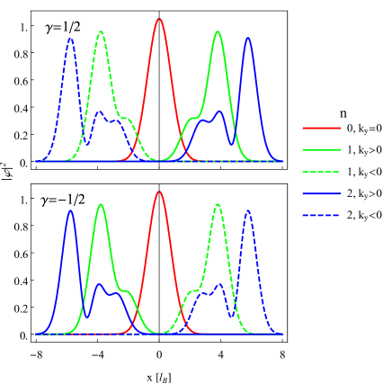
Figure 10: Probability density $\left|\varphi\left(x\right)\right|^{2}$ for $\xi=1$ (the $K$ valley), $B=1\,$T, and $\gamma=1/2$ (top) or $\gamma=-1/2$ (bottom).

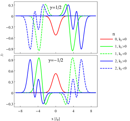
Figure 11: Current density $j_{y}(x)$ for $\xi=1$ (the $K$ valley), $B=1\,$T, and $\gamma=1/2$ (top) or $\gamma=-1/2$ (bottom).

Explicite forms of wavefunctions, given above by Eqs. (47) and (49), allows one to calculate the probability density $\left|\varphi\left(x\right)\right|^{2}$ (see Fig. 10) as well as the local current density $j_{y}=\varphi^{\dagger}\left(x\right)\cdot\sigma_{y}\cdot\varphi\left(x\right)$ (see Fig. 11).

As we have neglected the mass term throughout this Appendix, the physical quantities displayed in Figs. 10 and 11 are same for both valleys, $K$ and $K^{\prime}$, indicated by $\xi=1$ or $\xi=-1$ (respectively) in Eq. (28). Also, the probability density $\left|\varphi\left(x\right)\right|^{2}$ is affected by the direction of electric field, indicated by $\mbox{sgn}\,{\mathcal{E}}\equiv\mbox{sgn}\,\gamma$, only in a way that the two solutions for $n>0$, characterized by opposite wavenumbers ($k_{y}$ and $-k_{y}$) are exchanged upon $\gamma\rightarrow{}-\gamma$, see Fig. 10. In contrast, the current density $j_{y}(x)$ also changes sign upon $\gamma\rightarrow{}-\gamma$, see Fig. 11. Revisiting the derivation for $B<0$, one quickly can find that $\left|\varphi\left(x\right)\right|^{2}$ and $j_{y}(x)$ are affected by the magnetic field inversion ($B\rightarrow{}-B$) at fixed $\gamma$ in the same way as by the electric field inversion ($\gamma\rightarrow{}-\gamma$) at fixed $B$.

Another striking feature of the results presented in Fig. 11 is that for either the $n=0$ or $n>0$ modes, the total current (integrated over $x$) flows in one direction only, determined by the signs of ${\cal E}$ and $B$. For $n>0$, this can be attributed to the fact that solutions with $k_{y}>0$ and $k_{y}<0$ are localized at the opposite sides of a p-n interface, resulting in the same sign of the group velocity. For $n=0$, the solution given by Eq. (49) can be regarded as a linear combination of edge states from both sides of the interface, for which the current density is centered precisely at the interface line (as depicted scematically in Fig. 2 in the main text).

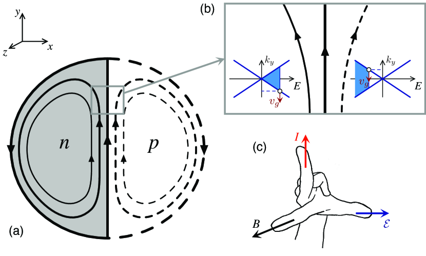
Figure 12: (a) Edge states in a finite disk-shaped graphene sample with a p-n interface in the quantum Hall regime (schematic). (b) A zoom-in of the interface region with band structure schemes. Open circles mark the two states on the Fermi level with opposite wavenumbers ($k_{y}<0$ and $k_{y}>0$) having equal group velocities ($v_{g}$). (Notice that the direction electric current is opposite to $v_{g}$ as the electron charge is $-e$.) (c) A version of the Fleming’s left hand rule showing mutual relation between directions of the magnetic field $B$, the in-plane electric field ${\cal E}$, and the current $I$ near the interface. The coordinate system used in Appendix B is also shown.

We comment now the relation between solutions for an infinite plane with trajectories depicted in Fig. 1.

The snake states (bottom panel in Fig. 1) can be represent as linear combinations of the solutions with $n=0$ and $n>0$, having a property that the full combination propagates in the same direction as each of its components. On the other hand, classical trajectores propagating in the direction (approximately) perpendicular to the interface (top panel in Fig. 1) represent finite-size effects having no analogs in an infinite plane. Most intriguing are the trajectories depicted in the middle panel of Fig. 1, propagating in both directions along the interface. Formally, this is possible since the total current, considered as a quadratic form, is neither positively nor negatively defined, and thus a generic quantum state composed of eigenstates with different $n$-s may also carry the current in opposite direction then each of the components.

In real sample of a finite size, edge states associated with a p-n junction derived in this Appendix are always accompanied by edge states close to a physical system boundary transporting the charge in opposite direction, see Fig. 12(a). When a disk-shaped sample is clamped with circular electrodes, forming the Corbino setup, edge currents are elliminated by the outer lead and the schematic current distribution for the lowest modes, visualized in Fig. 12(b), may be closely reproduced by the physical current density (see Fig. 6(a) in the main text). Remarkably, the familiar Fleming’s left hand rule, relating the directions of the current, the magnetic field, and the charge displacement (or the in-plane electric field) has also a version for graphene p-n junction in the quantum Hall regime, see Fig. 12(c).

Appendix C Mass confinement and the valley separation

We argue here that the mechanism behind spatial separation of currents in different valleys, appearing for a nonzero mass term (see Fig. 6(b) in the main text), can essentially be understood by analyzing the zero-energy wavefunction in the presence of infinite mass confimenent proposed in the seminal work by Berry and Mondragon Ber87 .

In the absence of electric field (${\cal E}=0$), a general zero-energy solution of Eq. (32) for $\xi=1$ (the $K$ valley) can be written as Pra07

$$\Phi_{0,k_{y},\xi=1}^{[{\cal E}=0]}(x)=C_{1}\left[\begin{array}[]{c}0\\ e^{-\chi^{2}/2}\end{array}\right]+C_{2}\left[\begin{array}[]{c}e^{\chi^{2}/2}\\ 0\end{array}\right],$$ (53)

with $C_{1}$ and $C_{2}$ being arbitrary complex numbers, and $\chi=l_{B}^{-1}x+l_{B}k_{y}$ again. For $\xi=-1$ (the $K^{\prime}$ valley), the two basis solutions on the right-hand side of Eq. (53) have interchanged spinor components.

Neglecting the intervalley scattering, one can show that confinement of the carriers in a bounded domain implies zero outward current at any point of the boundary at each valley ($\xi=\pm{}1$), namely

$$j_{{\bf n}(\alpha)}=\left\langle{}\xi\sigma_{x}\cos\alpha+\sigma_{y}\sin\alpha\right\rangle_{\Phi_{\xi}}=0,$$ (54)

where ${\bf n}(\alpha)=(\cos\alpha,\sin\alpha)$ is the unit vector normal to the boundary, and the spinor wavefunction $\Phi_{\xi}=\left(\Phi_{\xi,A},\Phi_{\xi,B}\right)^{T}$. Eq. (54) can be rewritten as

$$\xi\cos\alpha{}\,\mbox{Re}\left(\Phi_{\xi,A}^{\star}\Phi_{\xi,B}\right)+\sin\alpha\,\mbox{Im}\left(\Phi_{\xi,A}^{\star}\Phi_{\xi,B}\right)=0,$$ (55)

which is equivalent to

$$\left(\frac{\Phi_{\xi,B}}{\Phi_{\xi,A}}\right)^{\xi}=i{\cal B}\exp(i\alpha),$$ (56)

where ${\cal B}$ is real and depends on the physical nature of the confinement Ber87 .

Infinite mass confinement at $x=0$, restricting the wavefunction to the right hemiplane ($x>0$), corresponds to ${\cal B}=1$ and $\alpha=\pi$ in Eq. (56) and leads to the boundary condition

$$\left.\Phi_{\xi,A}\right|_{x=0}=i\xi\left.\Phi_{\xi,B}\right|_{x=0}.$$ (57)

Subsequently, the coefficients in Eq. (53) follow

$$C_{\xi,2}=i\xi{}C_{\xi,1}\exp\left(-k_{y}^{2}l_{B}^{2}\right).$$ (58)

The vertical current density for the zero-energy solution is

$$j_{y}=\left\langle{}\sigma_{y}\right\rangle_{\Phi_{0,k_{y},\xi}^{[{\cal E}=0]}}=-2\xi{}|C_{\xi,1}|^{2}\exp\left(-k_{y}^{2}l_{B}^{2}\right),$$ (59)

where the last equality follows from Eq. (58).

Clearly, the uniform current in Eq. (59) changes sign upon the valley exchange ($\xi\rightarrow{}-\xi$), providing a qualitative understanding of the valley separation, as the effect associated with zero-energy mode should overrule the effects originating from higher modes for a generic system close to the charge-neutrality point (allowing for $|k_{y}{}l_{B}|\ll{}1\,$).

References

- (1) M. Banerjee, M. Heiblum, V. Umansky, D. E. Feldman, Y. Oreg, and A. Stern, Observation of half-integer thermal Hall conductance, Nature (London) 559, 205 (2018).
- (2) D. F. Mross, Y. Oreg, A. Stern, G. Margalit, and M. Heiblum, Theory of Disorder-Induced Half-Integer Thermal Hall Conductance, Phys. Rev. Lett. 121, 026801 (2018).
- (3) C. W. J. Beenakker, C. Emary, M. Kindermann, and J. L. van Velsen, Proposal for Production and Detection of Entangled Electron-Hole Pairs in a Degenerate Electron Gas, Phys. Rev. Lett. 91, 147901 (2003).
- (4) J. R. Williams, L. Dicarlo, and C. M. Marcus, Quantum hall effect in a gate-controlled p-n junction of graphene, Science 317, 638 (2007).
- (5) D. A. Abanin and L. S. Levitov, Quantized transport in graphene p-n junctions in a magnetic field, Science 317, 641 (2007).
- (6) P. Carmier, C. Lewenkopf, and D. Ullmo, Semiclassical magnetotransport in graphene n-p junctions, Phys. Rev. B 84, 195428 (2011).
- (7) K. Zimmermann, A. Jordan, F. Gay, K. Watanabe, T. Taniguchi, Z. Han, V. Bouchiat, H. Sellier, and B. Sacépéa, Tunable transmission of quantum Hall edge channels with full degeneracy lifting in split-gated graphene devices, Nat. Commun. 8, 14983 (2017).
- (8) C. Qi, L. Ouyang, and J. Hu, Realizing robust large-gap quantum spin Hall state in 2D HgTe monolayer on insulating substrate, 2D Mater. 5, (2018).
- (9) M. Fujita, K. Wakabayashi, K. Nakada, and K. Kusakabe, Peculiar localized state at zigzag graphite edge, J. Phys. Soc. Japan 65, 1920 (1996).
- (10) K. Nakada, M. Fujita, G. Dresselhaus, and M. S. Dresselhaus, Edge state in graphene ribbons: Nanometer size effect and edge shape dependence, Phys. Rev. B 54, 1795 (1996).
- (11) E. Colomés and M. Franz, Antichiral Edge States in a Modified Haldane Nanoribbon, Phys. Rev. Lett. 120, 086603 (2018).
- (12) J. R. Schaibley, H. Yu, G. Clark, P. Rivera, J. S. Ross, K. L. Seyler, W. Yao, and X. Xu, Valleytronics in 2D materials, Nat. Rev. Mater. 1, 16055 (2016).
- (13) A. Rycerz, J. Tworzydło, and C. W. J. Beenakker, Valley filter and valley valve in graphene, Nat. Phys. 3, 172 (2007).
- (14) A. Rycerz, Nonequilibrium valley polarization in graphene nanoconstrictions, phys. stat. sol. (a) 205, 1281 (2008).
- (15) D. Gunlycke and C. T. White, Graphene Valley Filter Using a Line Defect, Phys. Rev. Lett. 106, 136806 (2011).
- (16) A. R. Akhmerov, J. H. Bardarson, A. Rycerz, and C. W. J. Beenakker, Theory of the valley-valve effect in graphene nanoribbons, Phys. Rev. B 77, 205416 (2008).
- (17) M. Wimmer, I. Adagideli, S. Berber, D. Tománek, and K. Richter, Spin Currents in Rough Graphene Nanoribbons: Universal Fluctuations and Spin Injection, Phys. Rev. Lett. 100, 177207 (2008).
- (18) F. Zhai, Y. Ma, and Y.-T. Zhang, A valley-filtering switch based on strained graphene, J. Phys.: Condens. Matter 23, 385302 (2011).
- (19) Y. Jiang, T. Low, K. Chang, M. I. Katsnelson, and F. Guinea, Generation of Pure Bulk Valley Current in Graphene, Phys. Rev. Lett. 110, 046601 (2013).
- (20) M. Settnes, S. R. Power, M. Brandbyge, and A.-P. Jauho, Graphene Nanobubbles as Valley Filters and Beam Splitters, Phys. Rev. Lett. 117, 276801 (2016).
- (21) S. P. Milovanović and F. M. Peeters, Strain controlled valley filtering in multi-terminal graphene structures, Appl. Phys. Lett. 109, 203108 (2016).
- (22) X.-P. Zhang, C. Huang, and M. A. Cazalilla, Valley Hall effect and nonlocal transport in strained graphene, 2D Mater. 4, 024007 (2017).
- (23) Y. Zhang, B. Guo, F. Zhai, and W. Jiang, Valley-polarized edge pseudomagnetoplasmons in graphene: A two-component hydrodynamic model, Phys. Rev. B 97, 115455 (2018).
- (24) A. Pályi and G. Burkard, Disorder-Mediated Electron Valley Resonance in Carbon Nanotube Quantum Dots, Phys. Rev. Lett. 106, 086801 (2011).
- (25) S.-g. Cheng, H. Liu, H. Jiang, Q.-F. Sun, and X. C. Xie, Manipulation and Characterization of the Valley-Polarized Topological Kink States in Graphene-Based Interferometers, Phys. Rev. Lett. 121, 156801 (2018).
- (26) A. Schroer, P. G. Silvestrov, and P. Recher, Valley-based Cooper pair splitting via topologically confined channels in bilayer graphene, Phys. Rev. B 92, 241404(R) (2015).
- (27) H. Pan, X. Li, F. Zhang, and S. A. Yang, Perfect valley filter in a topological domain wall, Phys. Rev. B 92, 041404(R) (2015).
- (28) Gorbachev, R. et al. Detecting topological currents in graphene superlattices, Science 346, 448 (2014).
- (29) K. F. Mak, K. L. McGill, J. Park, and P. L. McEuen, The valley Hall effect in MoS2 transistors, Science 344, 1489 (2014).
- (30) Y. Shimazaki, M. Yamamoto, I. V. Borzenets, K. Watanabe, T. Taniguchi, and S. Tarucha, Generation and detection of pure valley current by electrically induced Berry curvature in bilayer graphene, Nat. Phys. 11, 1032 (2015).
- (31) P. Rickhaus, P. Makk, M.-H. Liu, E. Tóvári, M. Weiss, R. Maurand, K. Richter, and C. Schönenberger, Snake trajectories in ultraclean graphene p-n junctions, Nat. Comm. 6, 6470 (2015).
- (32) P. Makk, C. Handschin, E. Tovari, K. Watanabe, T. Taniguchi, K. Richter, M.-H. Liu, and C. Schonenberger, Coexistence of classical snake states and Aharonov-Bohm oscillations along graphene p-n junctions, Phys. Rev. B 98, 035413 (2018).
- (33) Y. Liu, R. P. Tiwari, M. Brada, C. Bruder, F. V. Kusmartsev, and E. J. Mele, Snake states and their symmetries in graphene, Phys. Rev. B 92, 235438 (2015).
- (34) A. Rycerz, Magnetoconductance of the Corbino disk in graphene, Phys. Rev. B 81, 121404(R) (2010).
- (35) M. I. Katsnelson, Aharonov-Bohm effect in undoped graphene: Magnetotransport via evanescent waves, Europhys. Lett. 89, 17001 (2010).
- (36) E. C. Peters, A. J. M. Giesbers, M. Burghard, and K. Kern, Scaling in the quantum Hall regime of graphene Corbino devices, Appl. Phys. Lett. 104, 203109 (2014).
- (37) M. Kumar, A. Laitinen, and P. Hakonen, Unconventional fractional quantum Hall states and Wigner crystallization in suspended Corbino graphene, Nature Commun. 9, 2776 (2018).
- (38) Related to the local carrier concentration via , with being the wave vector.
- (39) For , quantum effects dominate and may fully elliminate the moderate-field range (see midle panel in Fig. 1) for smaller disks. As is related to the carrier concentration, particular scenario of the classical-to-quantum transition also depends on the electrostatic potential profile.
- (40) Katsnelson, M. I., Graphene: Carbon in Two Dimensions. (Cambridge University Press, Cambridge, 2012), Chapter 1.
- (41) D. W. Boukhvalov and M. I. Katsnelson, Chemical functionalization of graphene, J. Phys.: Condens. Matter, 21, 344205 (2009).
- (42) D. Haberer, D. V. Vyalikh, S. Taioli, B. Dora, M. Farjam, J. Fink, D. Marchenko, T. Pichler, K. Ziegler, S. Simonucci, M. S. Dresselhaus, M. Knupfer, B. Büchner, and A. Grüneis, Tunable Band Gap in Hydrogenated Quasi-Free-Standing Graphene, Nano Lett. 10, 3360 (2010).
- (43) J. Hong, E. Bekyarova, W. A. de Heer, R. C. Haddon, and S. Khizroev, Chemically Engineered Graphene-Based 2D Organic Molecular Magnet, ACS Nano 7, 10011 (2013).
- (44) B. Sachs, T. O. Wehling, M. I. Katsnelson, and A. I. Lichtenstein, Adhesion and electronic structure of graphene on hexagonal boron nitride substrates, Phys. Rev. B 84, 195444 (2011),
- (45) M. Yankowitz, J. Xue, and B. J. LeRoy, Graphene on hexagonal boron nitride, J. Phys.: Condens. Matter 26, 303201 (2014).
- (46) G. Rut and A Rycerz, Trigonal warping, pseudodiffusive transport, and finite-system version of the Lifshitz transition in magnetoconductance of bilayer graphene Corbino disks, Phys. Rev. B 93, 075419 (2016).
- (47) R. Landauer, Electrical resistance of disordered one-dimensional lattices, Phil. Mag. 21, 863 (1970).
- (48) M. Büttiker, Scattering theory of current and intensity noise correlations in conductors and wave guides, Phys. Rev. B 46, 12485 (1992).
- (49) For T the Zeeman splitting is meV [with and the Bohr magneton] and cannot affect the filter operation appearing at the potential and mass-term amplitudes of meV.
- (50) M. Müller, J. Schmalian, and L. Fritz, Graphene: A Nearly Perfect Fluid,, Phys. Rev. Lett. 103, 025301 (2009).
- (51) A. Lucas and K. C. Fong, Hydrodynamics of electrons in graphene, J. Phys.: Condens. Matter 30, 053001 (2018).
- (52) V. Lukose, R. Shankar, and G. Baskaran, Novel Electric Field Effects on Landau Levels in Graphene, Phys. Rev. Lett. 98, 116802 (2007).
- (53) A. Shytov, M. Rudner, N. Gu, M. Katsnelson, and L. Levitov, Atomic collapse, Lorentz boosts, Klein scattering, and other quantum-relativistic phenomena in graphene, Sol. State Comm. 149, 1087 (2009).
- (54) C. W. J. Beenakker, Andreev reflection and Klein tunneling in graphene, Rev. Mod. Phys. 80, 1337 (2008).
- (55) M. Wimmer, Quantum transport in nanostructures: From computational concepts to spintronics in graphene and magnetic tunnel junctions, PhD Thesis, Regensburg University, Germany (2009), Chapter 6.
- (56) J. H. Bardarson, J. Tworzydło, P. W. Brouwer, and C. W. J. Beenakker, Demonstration of one-parameter scaling at the Dirac point in graphene, Phys. Rev. Lett. 99, 106801 (2007).
- (57) A. Rycerz, Random matrices and quantum chaos in weakly-disordered graphene nanoflakes, Phys. Rev. B 85, 245424 (2012).
- (58) R. L. Burden and J. D. Faires, Numerical Analysis, (Brooks/Cole, Boston 2011), Chapter 5.
- (59) N. M. R. Peres and E. V. Castro, Algebraic solution of a graphene layer in transverse electric and perpendicular magnetic fields, J. Phys.: Condens. Matter 19, 406231 (2007).
- (60) D. Nath and P. Roy, Dirac oscillator in perpendicular magnetic and transverse electric fields, Ann. Phys. 351, 13 (2014).
- (61) M. Abramowitz and I. A. Stegun (eds.), Handbook of Mathematical Functions, (Dover Publications, New York, 1965), Chapter 19.
- (62) A. H. MacDonald, Quantized Hall conductance in a relativistic two-dimensional electron gas, Phys. Rev. B 28, 2235 (1983).
- (63) M. V. Berry and R. I. Mondragon, Neutrino billiards: time-reversal symmetry-breaking without magnetic fields, Proc. R. Soc. A 41, 53 (1987).
- (64) E. Prada, P. San-Jose, B. Wunsch, and F. Guinea, Pseudo-diffusive magnetotransport in graphene, Phys. Rev. B 75, 113407 (2007).