Hamiltonian Learning for Quantum Error Correction
Abstract
The efficient validation of quantum devices is critical for emerging technological applications. In a wide class of use-cases the precise engineering of a Hamiltonian is required both for the implementation of gate-based quantum information processing as well as for reliable quantum memories. Inferring the experimentally realized Hamiltonian through a scalable number of measurements constitutes the challenging task of Hamiltonian learning. In particular, assessing the quality of the implementation of topological codes is essential for quantum error correction. Here, we introduce a neural net based approach to this challenge. We capitalize on a family of exactly solvable models to train our algorithm and generalize to a broad class of experimentally relevant sources of errors. We discuss how our algorithm scales with system size and analyze its resilience towards various noise sources.
I Introduction
While finding an eigenstate of a given Hamiltonian might be a daunting task, the problem is nevertheless well defined and can often be solved by a set of existing tools. The inverse question, the identification of a Hamiltonian given the knowledge of a state , is a much more complicated one and without a unique answer in the general case.
Hamiltonian engineering is one of the central objectives in the context of constructing quantum information processing and storage devices LaddJelezko2010 ; Preskill2018NISQ ; AcinBloch2018 . Despite significant progress of quantum technologies over the last decades, the validation of the engineered Hamiltonian will always be an essential step for any quantum device. Moreover, the implemented Hamiltonian cannot be accessed directly, but only through the measurements performed on the system. Given these measurements one would like to verify that the desired Hamiltonian has been implemented correctly. In addition to that, this verification should ideally be done in an efficient and scalable way.
Reconstructing the Hamiltonian governing the systems’ dynamics directly from the measurement results constitutes the inverse problem we address. Beyond not being unique, in the quantum setting there arises an additional challenge due to the exponential size of the Hilbert space: Reconstructing even just the state alone via full quantum tomography is in general exponentially costly NielsenChuang2000 (though there are notable cases where tomography can be done efficiently TorlaiMazzola2018 ; CramerPlenio2010 ; GrossLiu2010 ). However, even with one eigenstate fully reconstructed, we still do not have enough information to determine which Hamiltonian it belongs to in the general setting.
There are two aspects one can exploit to simplify the inverse problem. First, we are typically not interested in the full Hamiltonian. For many purposes we only need to make sure we implement a Hamiltonian which possesses a ground state with desired properties, such as topological ground state degeneracies Kitaev2003 . In other words, we only aim at finding a possible parent Hamiltonian to this ground state family. Second, the implemented Hamiltonian we try to reconstruct will typically be in the vicinity of the sought after parent Hamiltonian. This property can render the reconstruction feasible and will typically not require a full tomography.
In this work, we develop a method to recover a parent Hamiltonian for a generic example important in the context of quantum devices: the family of the so-called stabilizer Hamiltonians Gottesman1997 that lie at the heart of the theory of fault-tolerant quantum computation LidarBrun2013 ; Gottesman1998 . A canonical example of this family of Hamiltonians is the toric code model Kitaev2003 . The toric code is a quantum spin- model defined on square lattice with periodic boundary conditions. Its ground state manifold is exactly known and its structure can be used for a stable encoding of quantum states.
In particular, we design a machine learning driven method for the validation of the implementation of the toric code. Our approach addresses all of the aforementioned challenges in the solution of the inverse problem: (i) We find a minimal set of local measurements performed on a ground state that allows us to learn the system’s Hamiltonian, i.e., we don’t need full tomography. (ii) Capitalizing on the proximity to the targeted toric code Hamiltonian we can train the neural network on a restricted class of exactly solvable models. Using the power of generalization of machine learning algorithms, we can then apply these trained networks to the general problem. (iii) The need for only a very restricted set of measurements and the use of efficient computing algorithms allow us to scale the solution problem beyond system sizes required for future experiments. Moreover, the generalization power of neural nets equips our approach with a certain resilience to experimental noise.
Our work has to be seen in the context of recent developments in the field. Specifically, using a trusted quantum simulator GranadeFerrie2012 ; WiebeGranade2014 ; WiebeGranade2015 ; WangPaesani2017 , determining a Hamiltonian from eigenstate dynamics BurgarthMaruyama2009 ; DiPaternostro2009 ; ZhangSarovar2014 ; DeOswald2016 ; VinetZhedanov2011 ; SoneCappellaro2017 ; WangDong2018 , compressed sensing RudingerJoynt2015 , RBM quantum tomography KieferovaWiebe2017 , maximum-likelihood generalizationKappen2018 , and mapping on straightforward parameter estimation problem GreplovaAndersen2017 have been used to address the inverse problem. Recently, methods to recover a local Hamiltonian based on measurements on a single eigenstate have been proposed QiRanard2017 ; ChertkovClark2018 ; GreiterSchnells2018 ; BaireyArad2019 . The introduced frameworks, however, come either with the necessity to measure long-range correlators or are not applicable to Hamiltonians consisting of commuting terms BaireyArad2019 .
The ability to efficiently validate Hamiltonians with topologically protected ground state degeneracies has direct implications for quantum error correction LidarBrun2013 ; FoselTighineanu2018 . One way of using the toric code as a quantum memory is to prepare the ground state in order to encode logical qubits in its ground state manifold Kitaev2003 . In practice, this means designing the many-body interactions that the stabilizer Hamiltonians contains. While many-body interactions can be difficult to implement in general in an experiment, there are theoretical proposals and experimental progress towards achieving the four-body interaction needed for the toric code in a variety of platforms BravyiSuchara2014 ; ChancellorZohren2017 ; MezzacapoLamata2014 ; MullerHammerer2011 ; MizelLidar2004 ; GurianCheinet2012 ; GladchenkoOlaya2009 ; BarreiroMuller2011 . However, only through the reliable validation of these schemes can one lift these proposals to a potential avenue for topologically protected quantum memories. Here we provide such a validation protocol.
In an alternative approach to using the toric code, one arrives at a ground state without the need to engineer any Hamiltonian, but an arbitrary state is successively projected into the desired state by a series of projective measurements FowlerMariantoni2012 ; ReiterSorensen2017 . The performance of these methods depends on the frequency, correlations and types of errors FowlerWhiteside2012 ; BravyiDuclos2012 ; DennisKitaev2002 ; SwekeKesselring2018 ; Andreasson2018 and we comment below how our algorithm relates these approaches.
This paper is organized as follows: In Sec. II we discuss the family of exactly solvable stabilizer Hamiltonians and the phase transitions they manifest. Sec. III addresses the neural network based Hamiltonian learning scheme we designed for this class of topological models. In Sec. IV we present the numerical analysis of the convergence and errors of the model and elaborate on its resilience to experimental noise. We discuss our results presented here in the broader context of the field and their implication for the future research directions in Sec V.
II Solvable topological models
Kitaev’s toric code model Kitaev2003 is defined on a square lattice with periodic boundary conditions and spin- degrees of freedom located on the edges. The Hamiltonian consists of the sum of four-spin interaction terms
| (1) |
where the stabilizer operators are defined as
| (2) | ||||
| (3) |
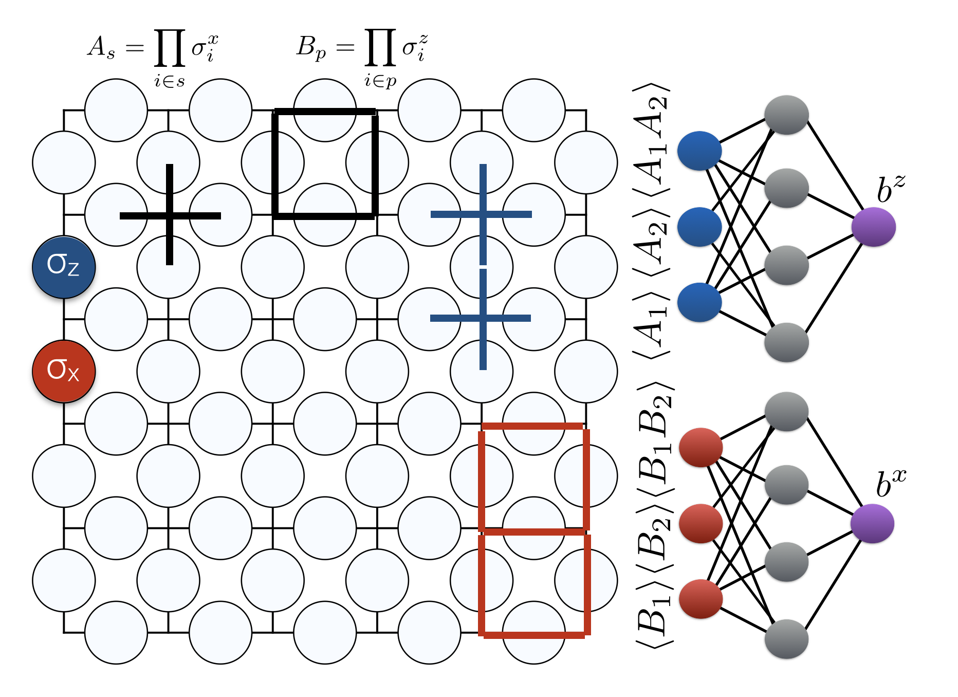
Here, denotes the set of four spins around a vertex and the set of four spins around a plaquette, respectively (see Fig. 1). Since the stabilizer operators, and , mutually commute, the ground state manifold is exactly known. It corresponds to eigenstates of all operators and with maximal eigenvalues .
The ground state degeneracy depends on the topology of the manifold the model is defined on. On a torus, there are four degenerate ground states , . Moreover, the topological order of these ground states results in stability of the degeneracy against arbitrary local perturbations. A qubit state can then be encoded through a suitably chosen superposition
| (4) |
The quantum operations on this state can be performed by so-called non-contractible loops, open strings of or operators accross the lattice. This property of the toric code ground state provides exceptionally stable encoding for the state of a logical qubit: A lattice-size long string of qubits needs to be flipped for the state of the logical qubit to change. For the purpose of our Hamiltonian learning we can restrict the discussion to one of the four states and we will use
| (5) |
where is a reference state of the lattice with all spins up. We comment below on why our method is insensitive to the choice made here.
A question can be posed about how the ground state changes if the stabilizer Hamiltonian is perturbed. In Refs. CastelnovoChamon2008 ; TsomokosOsborne2011 it was shown that there exists a way to leave the topologically ordered toric code phase while keeping the model analytically solvable. In particular, we can add -terms to the star operators, , in a way that slightly modifies the ground state, while keeping its degeneracy untouched. We write this Hamiltonian as
| (6) |
where . The positive, real-valued parameter drives the phase transition out of the topological phase.
The particular position of the phase transition depends on the distribution of fields given by . The ground state of can be expressed in terms of the original toric code ground state, as
| (7) |
The normalization factor is given and explained in Appendix A. The above described modification is not the only approach for keeping the Hamiltonian (1) analytically solvable while driving the phase transition. For example, we can symmetrically modify the plaquette terms, by -terms. In particular, adding to each plaquette would yield an analogous analytical ground state, .
The added perturbations are of experimental relevance, as they simplify to small (or ) background fields when Eq. (6) is expanded to lowest order in . Similarly, one obtains (or ) background fields if the field configuration is sufficiently sparse (see Appendix A). This effect could be a result of an imperfection or systematic errors in an engineered interaction.
For the sake of Hamiltonian learning, understanding the phase transition of model (6) is of central importance. Given the analytical form (7), it seems obvious that from suitably chosen measurements one should be able to infer the parameters of the Hamiltonian. However, this one-to-one correspondence might be obstructed by the set of degenerate ground states. It turns out, that as long as we are in a phase adiabatically connected to the pure toric code the Hamiltonian can be recovered independently of the specific superposition of degenerate ground states.
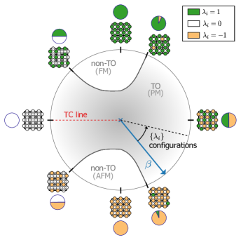
We show the position of phase transition in the perturbed toric Hamiltonian (6) pictorially in Fig. 2. The phase transition is found via mapping to classical spin models CastelnovoChamon2008 ; TsomokosOsborne2011 . In particular, if the corresponding classical model is in its paramagnetic phase we are in the phase of the toric code. Transitions out of this quantum phase are indicated by the ordering of the classical spins. Details about this mapping are provided in App. B. Stability against local perturbations is a known property of topological order. The phase diagram in Fig. 2 shows that topological order in Kitaev’s toric code model is also stable with respect to a large class of non-local perturbations.
These considerations lead to an immediate application to quantum error correction. Let us now assume four-body interactions of the toric Hamiltonian (1) are implemented in a chosen physical system. Consequently, the system will eventually arrive to its ground state. The sources of possible errors and inaccuracies are then systematic errors and noise inherently present in the experiment. We argue that error correction can then be performed at the level of Hamiltonian learning by finding a minimal set of measurements that has to be performed on the state at hand in order to deduce the Hamiltonian. Once the Hamiltonian is exactly found it can be corrected in order to arrive at the ideal Hamiltonian .
III Hamiltonian Learning
In order to solve the inverse problem we need to identify a minimal set of measurements that allows us to infer the faulty Hamiltonian. This requirement is intrinsically bound to the question of how we deduce the Hamiltonian from such measurements. In this section we outline how we approach this problem and how we can extend our scheme to the case of Hamiltonians where we do not have access to an exact ground state.
The measurements we need to perform to reconstruct the Hamiltonian should identify the product of field distributions given by with the parameter . To simplify the notation, we introduce the parameters to denote the product, .
Using translational invariance of the underlying lattice we find that the expectation values , ,, where corresponds to the chosen lattice site coordinate, contain a sufficient amount of information to recover the parameter .
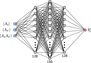
This observation implies that for each lattice site we need to evaluate correlation functions of the star operators, , “touching” at a given lattice site. The function that maps these expectation values on the Hamiltonian parameters is implemented via a small neural network, see Fig. 1. For each spin we input the expectation values , , and obtain that determines the field strength on a given spin.
We denote with the field strength of fields and with the fields strength of fields (which are determined from the expectation values of the plaquette terms , ,). As a consequence of symmetry under the exchange of vertices and plaquettes as well as and , the neural network trained to identify the field parameter also succeeds in identifying the parameter .
Assuming access to many copies of the system, one can evaluate the expectation values described above. Note that the total amount of expectation values needed scales linearly with the number of parameters to be estimated and hence, linearly with the number of spins in the lattice.
We train a small neural net on the exact ground states of the family of Hamiltonians (6). Owing to the analytical solution we are able to simulate lattices of almost arbitrary size. We choose a particular spin in the lattice and evaluate the expectation values , , for a range of different field distributions on the surrounding spin and a range of values of .
We restrict ourselves to the field configurations such that the system is in the toric code phase, cf. Fig. 2. Consequently, it is possible to recover the Hamiltonian even if the system is in an arbitrary state in the ground state manifold, while the training set is restricted to a specific ground state. The reason for this simplification lies in the properties of the nature of the toric code ground state: The degenerate ground states can not be distinguished by local measurements and hence, the measurement outcome of the stabilizer expectation values is identical for all states in the ground state manifold.
We use the set of expectation values , , as the input for our neural net. The labels we train the network to associate with these inputs are the field strength on the given spin (Fig. 1). We find that a dense neural network of layers with , and neurons respectively is able to reliably approximate this mapping. We detail the architecture and details of the training in App. C.
We evaluate the performance of the network on states that lie outside of manifold of ground states of exactly solvable Hamiltonians. This strategy would in principle allow us to apply the trained models on measurements of a large quantum computer or simulator. Above, we introduced two examples of toric-code Hamiltonian modifications, one through and one through fields
| (8) |
Separately, these modifications do not violate exact solvability of the model. However, in the small- limit this Hamiltonian covers a very general set of errors that may occur in an actual quantum device. Therefore, we showcase our method on this Hamiltonian.
The above Hamiltonian cannot be solved for large systems. However, we can use the network trained on the solvable Hamiltonian. We then apply it to the ground state of (8) which for small system sizes can be obtained by brute force diagonalization.
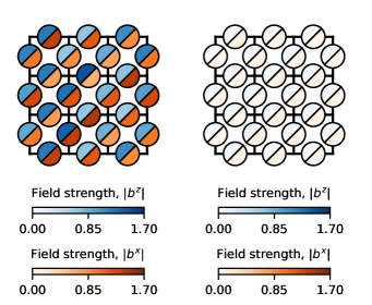
Let us introduce an iterative algorithm designed to evaluate the fields that characterize Hamiltonian (8). We take one of the above described ground states and evaluate the required correlators , , and , , for each of the spins, and we use them as input to the trained neural network. For each spin we obtain the magnitude of the field strength in and direction. We follow this step by numerically removing the found fields from the original input Hamiltonian. While in a numerical simulation this is a straightforward task, in a quantum simulation this would be implemented by adjusting the interaction parameters to cancel the fields and re-initializing, or by an adiabatic transition between two Hamiltonians. An implementation of the corresponding set of gates is also possible. We use the “corrected” state as the new input for the same neural network, remove the resulting fields, and repeat the procedure iteratively until convergence. The iterative application is not completely straightforward as and result in the same expectation values of and . Hence, the iterative procedure includes a decision tree for the sign of the field. With these adjustments (addressed in detail in Appendix C) the correct fields (and therefore the correct Hamiltonian) are found within five iterations. We illustrated the algorithmic field removal in Fig. 3.
IV Results
We define two quantities to characterize the performance of our method. First, we introduce a measure at the level of the resulting corrected quantum ground states: The probability that physical qubits pertain spin flip or phase errors after the projection onto the stabilizers. Second, we put forward a criterion at the level of the corrected Hamiltonian. This measure is simply a distance between the ideal and the corrected Hamiltonian in a suitably chosen metric.
To formulate the error measure for the corrected states we draw the connection to standard error correction strategies: One starts from an arbitrary quantum state and implements a projection on the eigenspaces of the operators , by measuring the state of ancillary qubits that are entangled with star and plaquette operators FowlerMariantoni2012 . This projection results in an eigenstate of Hamiltonian (1). Using the measurement outcomes, a decoder identifies single spin operations that map the state to the ground state of Hamiltonian (1). The decoder will succeed if the probability of spin and phase flip errors between the projective measurements is lower than a given threshold. This threshold ranges anywhere between - depending on the chosen error model FowlerWhiteside2012 ; BravyiDuclos2012 ; DennisKitaev2002 ; SwekeKesselring2018 ; BreuckmannNi2018 ; Ni2018 ; TorlaiMelko2017 ; Andreasson2018 .
For our case we do not start from an arbitrary state, but from the ground state of the corrected parent Hamiltonian. We can relate the precision of our method to standard decoding techniques by calculating the probability that a single physical qubit will flip its spin or phase when projecting into the stabilizer eigenspace. The calculation of a single qubit spin or phase flip can be deduced from the stabilizer expectation values and and is detailed in App. D.
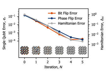
In Fig. 4, we show the probability of a single bit or phase flip error as a function of the iteration of our algorithm. The iteration axis also contains pictorial illustrations of the absolute field strengths on the state. When projecting on the stabilizer eigenstates from the original faulty eigenstate we find errors well above the decoding thresholds (typically above ). We are, thus, able to show that even a small systematic error present in the Hamiltonian engineering can potentially confuse a decoder. After five iterations we arrive to a single qubit error probability of order of .111This translates into the probability for wrong stabilizer measurements of the same order . In other words, if we attempted to decode the initial faulty ground state, the decoder may fail. After our correction procedure it is always highly likely to succeed.
Another measure that quantifies the precision of Hamiltonian learning can be implemented on the level of the Hamiltonian directly BaireyArad2019 . This method relies on expanding the family of Hamiltonians we would like to estimate in a suitable basis and then measure the distance of the estimated coefficients from the ideal ones. In particular, the Hamiltonian is expressed as , where is an operator basis with expansion coefficients . Once we make sure that the chosen basis is independent of the parameters to be estimated, the Hamiltonian error simply translates into the distance
| (9) |
where and are the normalized vectors of exact and found coefficients respectively. In our case are non-linear functions of , the parameters the neural network is estimating. We show this functional dependence together with the expansion of the Hamiltonian in App. D. The resulting Hamiltonian error is shown as a function of iterations of the protocol in Fig. 4. We normalize the Hamiltonian error such that the maximal value is one. After five iterations of the protocol, the distance between expansion coefficients decreases to order of .
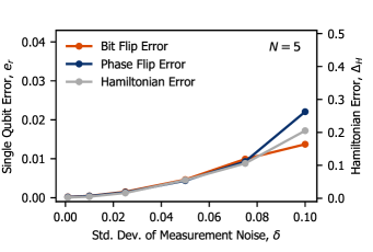
Both state and Hamiltonian error explained up to this point were evaluated under the assumption of perfect experimental readout. We now briefly discuss how our method performs when this assumption is relaxed. We assume that the experimental input for the neural network is in the form of the measured expectation values. Experimental noise would then enter through these expectation values not being evaluated correctly. Additionally, estimating an expectation value using a finite number of samples induces a statistical uncertainty. We simulated this scenario by adding Gaussian noise on our numerically evaluated inputs , . We show the behavior of the single qubit errors as well as the Hamiltonian error in Fig. 5. We observe that even in presence of Gaussian noise the single qubit error rate after projection onto the stabilizers is reliably reduced below .
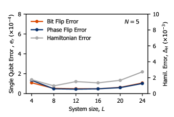
All simulations so far are conducted for a lattice with spins, as a full quantum simulation is required to simulate the correction procedure for the non-solvable model [see Eq. (8)]. However, this restriction is not necessary when it comes to training of the neural network. In an experiment, the presented Hamiltonian learning procedure can therefore be applied to almost arbitrary lattice sizes. We demonstrate the scaling behavior by training the network separately for different lattice sizes while the size of the training set is fixed. The computation time to generate the training set via Monte Carlo sampling only increases linearly with number of qubits, as the number of sweeps through the lattice is kept constant. The correction process can only be simulated by keeping the model solvable. We want to emphasize that this restriction appears purely for testing purposes and is not of relevance in an experimental setup. In Fig. 6 the results of our simulations are shown, i.e. the error measure outcomes are independent of lattice size.
V Discussion
In this work we have introduced a machine-learning driven method for scalable quantum Hamiltonian learning based on a toy model relevant for quantum information processing, the toric code. Scalability was achieved by training the neural network on exactly solvable models. We have shown that our method performs well even for states that lie outside this class of analytical solutions. Using knowledge of topological phases and the stability of the toric code to a large class of non-local perturbations, we justified the restriction of the correction to the topological phase. However, an expansion of the correction process outside of the topological phase should be a straightforward procedure.
Our work is complementary to standard approaches to quantum error correction. More specifically, the performance of a standard decoder is significantly improved when combined with the procedure introduced here. When the Hamiltonian is engineered precisely, logical errors are suppressed. We provided a tool for precise engineering based on measuring a minimal set of local expectation values scaling linearly with number of qubits. Implementing a practical protocol that incorporates both the Hamiltonian learning techniques presented here and stabilizer measurement based decoders would therefore be a natural step towards running a fault-tolerant quantum computations.
Acknowledgements
We acknowledge discussions with Aleksander Kubica, Tomas Jochym O’Connor, Gil Refael, Netanel Lindner, Christoph Bruder and Mohammad Hafezi. We are grateful for financial support from the Swiss National Science Foundation, the NCCR QSIT. This work has received funding from the European Research Council under grant agreement no. 771503. This research was supported in part by the National Science Foundation under Grant No. NSF PHY-1748958 and by the Swiss National Science Foundation under Grant No. 183945. AV acknowledges financial support of the ETH Master Scholarship Programme.
Appendix A Supplementary Calculations
The ground state structure in limiting cases of the disordered toric code model introduced throughout this work is detailed in this section.
A.1 Normalization factor
The ground state of the disordered Hamiltonian defined in Eq. (6) is of the form
| (10) |
To explain the normalization factor , we re-write the toric code ground state as
| (11) | ||||
| (12) | ||||
| (13) |
where denotes the abelian group whose elements are all possible spin-flip operations defined by the action of products of vertex operators on an initial spin-configuration CastelnovoChamon2008 . In the toric code, periodic boundary conditions in all directions are imposed leading to the relation . The group elements of the group are only determined modulo the factor . As a consequence, the number of elements in the group is equal to half the number of possible products of vertex operators. We can re-write the ground state using the introduced notation
| (14) |
Here, can take the values . More concretely, corresponds to the eigenvalue of the operator on the eigenstate . The normalization factor (partition function) has the following form
| (15) |
A.2 Disorder in the limit of small fields
In particular cases, the disorder defined in Eq. (6) simplifies to () single-spin fields. In the limiting case of small fields (), we expand the added term as
| (16) |
Terms of higher order containing , and are neglected as a result of the approximation. Hence, we arrive at a model containing only fields acting on single spins, and interactions between spins vanish. More specifically, the Hamiltonian of the disordered model in this limit is given by CastelnovoChamon2008
| (17) |
A.3 Disorder in the limit of sparse fields
A similar approximation can be made for sufficiently sparse fields. We denote with “sufficiently sparse” here a field configuration, where at most one field parameter per vertex is not equal to zero. If this condition is met, all interactions between spins vanish and only fields acting on single spins remain
| (18) |
The index denotes the spin in vertex for which . We insert this simplification into the Hamiltonian defined in Eq. (6) and arrive at
| (19) |
Here, is defined as the sparse set of spins with field strength . We conclude, that we arrive at a model consisting of the toric code model with fields and no additional interactions.
Appendix B Topological phases
We analyze topological order and phase transitions of the disordered toric code model in this section. For this purpose, we map the system to a classical spin model as done in CastelnovoChamon2008 . The ground state of the modified toric code (6) is given by [Eq. (14)]
| (20) |
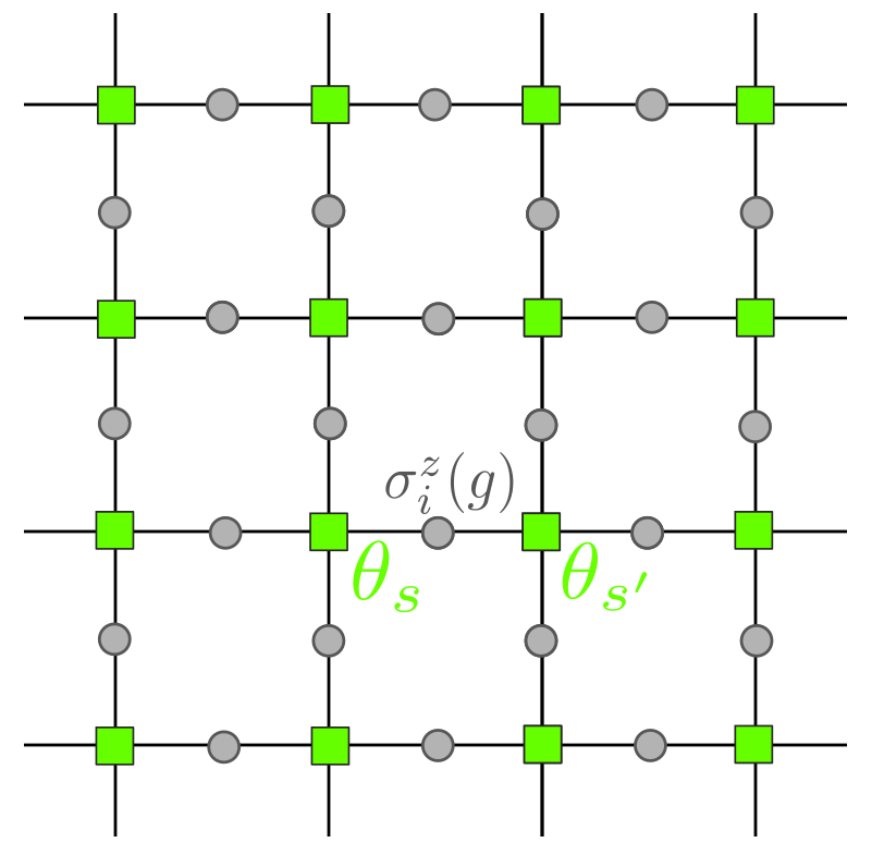
It should be noted, that the group element is only determined by the product modulo the product of all vertex operators, due to periodic boundary conditions. We can map every product of vertex operators to a pseudo-spin configuration, defined as follows: Artificial degrees of freedom are introduced on all vertices . The value of determines, if the vertex is flipped (contained in the product of vertex operators we map the pseudo-spin configuration to). More specifically, the vertex is flipped if . We can now make a change of variables. The eigenvalue of the spin depends on the two adjacent vertices being flipped or not. As a consequence, this eigenvalue is given by , resulting in a mapping between the the spin configuration and the pseudo-spin configuration with a gauge freedom of an overall factor of . The mapping is further illustrated in Fig. 7.
Let us define an Ising model on the pseudo-spin configuration with the Hamiltonian given by CastelnovoChamon2008 ; TsomokosOsborne2011
| (21) |
The connection to the field parameters and is given by the coupling constant . In particular, where is a product between the Boltzmann constant and the temperature . The edge with adjacent sites and is denoted by the index . An indication of a connection between the phase transition of the quantum model and the classical spin model can be obtained from the partition function of the defined Ising model
| (22) | ||||
| (23) |
By comparing to the partition function of the disordered toric code (15) model we observe that AbastoHamma2008 .
We can show that the phase transition of the disordered toric code is mapped to the phase transition of the Ising model by considering a well-known measure to detect quantum phase transitions, the fidelity susceptibility YouLi2007 . The fidelity susceptibility is defined as
| (24) |
Here, the state is a ground state of a given Hamiltonian depending on the parameter , for our case the state is defined in Eq. (7). A quantum phase transition is indicated via a maximum or divergence in the fidelity susceptibility VenutiZanardi2007 ; GuLin2009 . In particular, this property has been shown for generic second-order symmetry-breaking quantum phase transitions ZanardiPaunkovic2006 . It has further been suggested by numerical studies (AbastoHamma2008, ), that the fidelity susceptibility is also able to detect a topological phase transition. The fidelity susceptibility for the introduced disordered toric code model is calculated as
| (25) | |||
| (26) |
We can understand the connection between the phase transition of the quantum toric code model and the phase transition of the classical spin model by examining the heat capacity of the mapped Ising model
| (27) | ||||
| (28) |
We observe, that the heat capacity is proportional to the fidelity susceptibility of the disordered toric code model. A similar relation has already been found in AbastoHamma2008 for the fidelity metric, an equivalent measure to the fidelity susceptibility regarding the characterization of quantum phase transitions. For the disordered toric code model, both fidelity measures simplify to the same expression. As both the heat capacity and the fidelity susceptibility indicate a phase transition via a maximum or divergence respectively, we conclude that a phase transition in the classical spin model at a critical temperature indicates a quantum phase transition in the disordered toric code model at critical field strength .
We now understand, that a phase transition in the defined Ising model indicates a quantum phase transition of the disordered toric code model. It remains to examine, if the indicated quantum phase transition is topological, i.e. if the transition is made to a topologically trivial phase. This question has already been discussed in CastelnovoChamon2008 ; TsomokosOsborne2011 . In particular, it has been shown that the paramagnetic phase of the Ising model maps to the topological phase of the perturbed toric code model, whereas the ferromagnetic phase maps to the topologically trivial phase. The antiferromagnetic phase also maps to the topologically trivial phase due to sublattice symmetry. The argument for the mapping of Ising phases to topological phases holds only deep in the corresponding phases in the case of arbitrary field strengths. Combined with the discussion of the fidelity susceptibility, we can conclude that it also holds close to the phase transition and that the topological phase transition is sharp.
Let us examine, how the field configuration influences the position of the phase transition at critical field strength . A complete description is in general a daunting task due to the amount of degrees of freedom related to the field configuration . However, we can gain insights about the stability of the topological phase when focusing on a more conceptual - phase diagram (see Fig. 2). In particular, we aim to show for which field configurations phase transitions out of the topological phase occur at all.
In order to analyze the relation between field configuration and phase transition, we examine two limiting cases. We start with a configuration with . This configuration is mapped to an Ising model with equal bond strengths, for which the phase transition occurs at critical field strength . Let us ask a question whether we can modify the field configuration such that no phase transition occurs anymore. As long as all fields are strictly greater than , there can always be found a critical field strength such that the system leaves the topological phase. More concretely, the value of can always be chosen large enough such that every product of fields is larger than . Therefore, a phase transition must occur. Due to sublattice symmetry, the same statement holds for all fields strictly smaller than .
There are two options to arrive at a configuration where no phase transition occurs. This can be achieved by obtaining a configuration of neither only strictly positive nor only strictly negative fields. One option lies in setting a fraction of fields equal to and arriving at a mixture of strictly positive fields and fields equal to (or strictly negative fields and fields equal to ). Here, we can examine the critical concentration of fields, that have to be removed such that no phase transition occurs. In other words, we are interested how sparse the configuration has to be such that the topological phase is never left. To answer this question, we consider a well-known probabilistic classical spin model: an Ising model with random bond dilution. In particular, the Hamiltonian of the diluted Ising model is given by
| (29) | |||
| (30) |
corresponding to
Here, is the probability distribution of a bond strength, translating into the probability distribution of a field with denoting the edge connecting the sites and . The question of the critical fraction of fields set to zero hence corresponds to a critical dilution probability . The model has been well-studied HoneckerPicco2001 ; PiccoHonecker2006 ; RegerZippelius1986 ; GruzbergRead2001 and the critical concentration found to be . In other words, the presence of the background field on less than half of the spin cannot drive the system out of the topological phase regardless of the field strength.
Another way one can modify the field configuration in order to preserve topological order is to flip signs of a fraction of fields. We can make use of a probabilistic Ising model, which has already been studied in connection to the disordered toric code model TsomokosOsborne2011 . In this model, we consider a bond dilution determined by the probability distribution
| (31) |
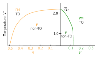
where is the probability that the sign of a bond strength is flipped. The critical value of has been found to be HoneckerPicco2001 ; PiccoHonecker2006 ; RegerZippelius1986 ; GruzbergRead2001 . Due to sublattice symmetry, the phase diagram for this model is symmetric with respect to . Hence, a second critical value occurs at . The phase diagram of both models is well-known and shown in Fig. 8.
The found relations between field configuration and phase transition are summarized into a conceptual phase diagram, shown in Fig. 2. The field configuration and the field strength are encoded as angle and amplitude in the phase diagram. The field distribution is varied continuously with change of angle in between the configurations explicitly marked in the diagram. The depicted configurations either mark a phase transition or correspond to a limiting case of field strengths. An exemplary field distribution and a small diagram indicating the percentages of occurring field strengths illustrate the depicted configurations. The field configurations on the left hand side do not contain fields of different signs simultaneously. On the right hand side, all fields are different from . The phase diagram is symmetric with respect to its horizontal axis as a result of sublattice symmetry.
Appendix C Neural Network
C.1 Network training and architecture
The architecture and training process of the artificial neural network used for the Hamiltonian learning process is detailed in this section. We have introduced in the main text a class of Hamiltonians of the form
| (32) |
Our algorithm aims at determination of the parameters and .
We found the measurement set used as an input for the network heuristically. This set is obtained by minimizing the amount of measurements containing sufficient information to determine the Hamiltonian parameters. The result of this search is the set of expectation values , and , that shows to be sufficient to determine the fields . Symmetry leads to the equivalent set of plaquette operators, , and determining fields . As a result, when the trained network receives as input the vertex stabilizer expectation values, it outputs the field on the qubit with adjacent vertices . Analogously, when given the inputs , and , it returns for qubit with adjacent plaquetter and . We can combine the ability of neural networks to generalize knowledge with the symmetry of the model with respect to exchange of vertices and plaquettes. It follows that it is sufficient to train on the solvable model containing only fields in one direction, and use the network for evaluation of the general non-solvable model. Even though the training is restricted to either vertex stabilizer expectation values or plaquette expectation values, the symmetry ensures that both types of expectation values can be taken as input for evaluation and consequently both field configurations and can be determined. We choose to train on the solvable model with -type fields
| (33) |
Thus, the network is trained on the inputs , and . It is furthermore sufficient to train for a field strength at a specific position (spin), as the measurements for a field at a different position are translationally invariant with respect to the position of the field. In other words, we just choose a single spin to evaluate the expectation values and create the training set by changing the size of the lattice and distribution of the background fields.
We design a neural network with three input neurons, three hidden layers and one output neuron. The network architecture is depicted in Fig. 9. As we estimate a continuous parameter, we calculate the loss function as mean squared distance between the estimated value and the correct field strength
| (34) |
where the vector corresponds to the field vector of the network output and labeled data respectively. The batch size is denoted by .
The network is trained separately for each lattice size , as the stabilizer expectation values vary with lattice size. Training data is generated by calculating the vertex stabilizer expectation values via Monte Carlo sampling for sufficiently distinct field configurations , such that the network learns to neglect the contribution in the expectation values from fields we do not aim to determine. More concretely, every field strength is taken from a uniformly random distribution in the interval and the label is chosen to be the absolute value of the field strength at position . The maximal value of the field strength is selected such that field configurations are included inducing a probability of a single qubit error after projection into the stabilizer eigenspace larger than the error threshold of standard decoders. We use a traning set of examples. The size of the training set is identical for all lattice sizes. We use this restriction in order to be able to analyze scaling behavior (see Fig. 6).
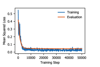
In Fig. 10, we show that training and evaluation loss (50 evaluation examples) both converge after less than training steps. The training results for the lattice length are plotted. We consider statistical uncertainty in the input expectation values as a main source for the non-zero loss the training converges to, which is similar for all tested lattice sizes. In particular, the neural network has been trained for the lattice sizes .
C.2 Determining the sign
We use a trained neural network to determine the absolute value of and by feeding in stabilizer expectation values. These expectation values do not contain sufficient information to determine the sign of and . In order to find the sign, for each spin we additionally measure the expectation values and . We show in the following, that the sign of the field strength can be approximated as the sign of the corresponding expectation value and . In particular, we demonstrate this approximation for a model containing fields in both directions with an additional restriction ensuring solvability. Exact diagonalization and application to the complete Hamiltonian learning process for the analytically non-solvable model discussed throughout this work confirms, that this decision mechnism to determine the sign holds approximately also for the generalized model. Let us examine the restriction added on the model to keep it solvable. For this purpose, we introduce the sets and , which denote the set of spins, for which and , respectively. We set . In different words, only a field in one direction can be present on each spin. The Hamiltonian is then given by
| (35) | |||
It can straightforwardly be verified that the un-normalized ground state is of the form
| (36) |
As we aim to determine a sign, we can ignore overall factors. Hence, we will not discuss normalization here. We calculate the sign of the expectation value measured on the introduced ground state with the restriction
| (37) |
Any overall factors occurring during the calculation are eliminated by the sign function . In particular, all dependencies on the parameters can be factorized to an overall factor using the condition and therefore vanish. In addition, we introduced the group as the subgroup containing all elements for which . Analogously, the group is defined such that for . The factors and are given by
We can relate the sign of the expectation value to the sign of the parameter by introducing the approximation 222The two factors are not exactly equal, as the spin is flipped as part of a vertex and not independently. As a consequence, the value of is correlated with the values of the remaining spins in the two adjacent vertices.. In addition, we make use of the fact that . Combining the two relations, we arrive at
where we dropped the overall factor . Henceforth, the relations
hold approximately. Symmetry implies the analogous relations for the parameter and the expectation value .
We can summarize the Hamiltonian learning process in two steps. In the first step, the stabilizer expectation values , , and , , are measured for each spin and the results fed into the trained neural network, which outputs the absolute values of the field configurations. In the second step, and are measured for each spin and the signs of the parameter determined correspondingly. With the obtained field strengths, the system can be corrected towards the pure toric code. The process can be iterated to achieve optimal results.
Appendix D Error measures
D.1 Probability of a single qubit error
On the level of quantum states, we have introduced as an error measure the probability that a single qubit flips its spin or phase after projection into the stabilizer eigenspace. In particular, this probability allows to assess the improvement our introduced method can in principle bring to quantum error correction. More concretely, if the calculated probability is reduced below the decoder-specific threshold, the performance of a standard decoder applied to the system is significantly improved. Let us make two clarifications to refine the relation to quantum error correction. The single qubit error threshold is usually defined with respect to the probability of a single qubit error per correction cycle FowlerWhiteside2012 ; BravyiDuclos2012 ; DennisKitaev2002 ; FoselTighineanu2018 ; SwekeKesselring2018 , where a correction cycle corresponds to measurements of stabilizers and applied single-qubit gates. Here, we examine a single cycle and hence, it is sufficient to calculate the probability of a single qubit error. In addition, the examined disorder throughout this work is not of the form of single qubit spin- or phase flip errors. Nevertheless, any disorder is translated to spin- and phase flip errors by projective measurements of the stabilizers. Consequently, we explain in this section how to calculate the single qubit error probability after projecting into the toric eigenspace.
Instead of simulating the projective measurements and “counting” the single qubit errors, we calculate the single qubit error probability in a way that does not rely on full quantum simulation and is hence also accessible for large lattice sizes.
We determine the probability of a physical phase-flip (spin-flip), by calculating as first step the probability for an arbitrary vertex (plaquette) to be flipped and deducing the single qubit error probability. We explain the calculation on the example of vertex flips and single qubit phase-flip errors. It can be repeated analogously for the case of plaquette flips and single qubit bit-flip errors.
Calculating the stabilizer flip rate
We deduce the vertex stabilizer flip rate using the expectation values , which have already been calculated during the Hamiltonian learning procedure. Every vertex has the eigenvalues . Thus, we can make an approximation and re-write a vertex expectation value as
| (38) |
Here, the probability of the vertex to be flipped (projected into an eigenstate with eigenvalue ) is given by . We invert the relation to find the probability
| (39) |
To obtain an average vertex flip rate , we average over all vertices
| (40) |
Calculating the error rate
We now understand how to obtain the probability of a vertex flip. We proceed by using the vertex flip probability to deduce the probability of a single qubit phase flip as follows.
We calculate the vertex flip rate for different probabilities of a single qubit phase flip by numerically sampling. In particular, we start with a lattice where no phase is flipped and flip each phase with probability . The vertex flip probability is obtained by repeating the procedure, counting the number of flipped vertices and averaging. We arrive at a function . The inverse function and as a result the probability of a single qubit error can be found by numerical regression.
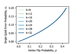
The function is independent of lattice size in the parameter range we are considering here. We verified this by calculating the vertex flip probability for the single qubit phase flip probabilities for the lattice sizes , where the total number of spins is equal to (see Fig. 11).
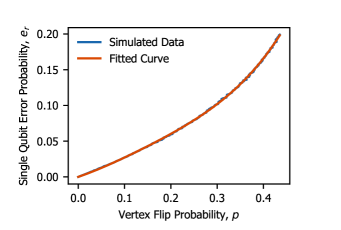
We can conclude that it is sufficient to find a numerical fit for the function of one lattice size. To minimize uncertainties caused by the statistical error of the simulation, we pick the largest simulated lattice size, , to fit the curve. We use an ansatz of a polynomial of degree and minimize the mean squared distance. The curve is fitted up to a mean squared loss of by the function
| (41) |
Both numerically simulated data and the fit are shown in Fig. 12. The obtained function returns the probability of a single qubit phase flip given the vertex stabilizer expectation values and similarly applies to single qubit bit-flip errors given plaquette expectation values. Full quantum simulation for confirms these results.
D.2 Measure for Hamiltonian error
An error measure on the level of Hamiltonian learning is given by the reconstruction error BaireyArad2019 . In this section, we detail the calculation of this Hamiltonian error for the disordered toric code model. As a reminder, is given by (9)
| (42) |
where the vector corresponds to the normalized coefficient vector . The coefficients are obtained by expanding the Hamiltonian in a suitable basis
| (43) |
where all parameters we estimate are contained in the coefficients, not in the basis. Let us expand the disordered toric Hamiltonian in an operator basis
| (44) |
Each term in the expansion of the Hamiltonian is a product of the form , with being a coefficient and an operator. The dependence on the parameters and is fully contained in the coefficients , the operator basis is independent of the parameters. More specifically, the operator basis resulting from the Hamiltonian expansion is a combination of the unit matrix and products of Pauli matrices. We illustrate the separation into coefficients and basis by re-writing all occurring operators as , an (arbitrarily) numbered basis element. The expansion of the Hamiltonian can be divided in two parts: a sum over all vertices and a sum over all plaquettes . For a simpler basis numbering, all basis elements (operators) occuring in the sum over vertices are denoted by and the operators in the sum over plaquettes are denoted by . Inserting the basis elements yields
| (45) | |||
| (46) |
The field parameters and only occur in the coefficients . The operator basis is the joined set of the basis elements contained in and in . Similarly, the coefficients are given by = and can be read off easily. Having hereby deduced the coefficients from the field parameters and , we can calculate the Hamiltonian error using Eq. (42).
References
- [1] Thaddeus D Ladd, Fedor Jelezko, Raymond Laflamme, Yasunobu Nakamura, Christopher Monroe, and Jeremy Lloyd O’Brien. Quantum computers. Nature, 464(7285):45, 2010.
- [2] John Preskill. Quantum computing in the nisq era and beyond. Quantum, 2:79, 2018.
- [3] Antonio Acín, Immanuel Bloch, Harry Buhrman, Tommaso Calarco, Christopher Eichler, Jens Eisert, Daniel Esteve, Nicolas Gisin, Steffen J Glaser, Fedor Jelezko, et al. The quantum technologies roadmap: a european community view. New Journal of Physics, 20(8):080201, 2018.
- [4] Michael A Nielsen and Isaac L Chuang. Quantum information and quantum computation. Cambridge: Cambridge University Press, 2(8):23, 2000.
- [5] Giacomo Torlai, Guglielmo Mazzola, Juan Carrasquilla, Matthias Troyer, Roger Melko, and Giuseppe Carleo. Neural-network quantum state tomography. Nature Physics, 14(5):447, 2018.
- [6] Marcus Cramer, Martin B Plenio, Steven T Flammia, Rolando Somma, David Gross, Stephen D Bartlett, Olivier Landon-Cardinal, David Poulin, and Yi-Kai Liu. Efficient quantum state tomography. Nature communications, 1:149, 2010.
- [7] David Gross, Yi-Kai Liu, Steven T Flammia, Stephen Becker, and Jens Eisert. Quantum state tomography via compressed sensing. Physical review letters, 105(15):150401, 2010.
- [8] A Yu Kitaev. Fault-tolerant quantum computation by anyons. Annals of Physics, 303(1):2–30, 2003.
- [9] Daniel Gottesman. Stabilizer codes and quantum error correction. Caltech Ph. D. PhD thesis, Thesis, eprint: quant-ph/9705052, 1997.
- [10] Daniel A Lidar and Todd A Brun. Quantum error correction. Cambridge university press, 2013.
- [11] Daniel Gottesman. Theory of fault-tolerant quantum computation. Physical Review A, 57(1):127, 1998.
- [12] Christopher E Granade, Christopher Ferrie, Nathan Wiebe, and David G Cory. Robust online hamiltonian learning. New Journal of Physics, 14(10):103013, 2012.
- [13] Nathan Wiebe, Christopher Granade, Christopher Ferrie, and David G Cory. Hamiltonian learning and certification using quantum resources. Physical review letters, 112(19):190501, 2014.
- [14] Nathan Wiebe, Christopher Granade, and David G Cory. Quantum bootstrapping via compressed quantum hamiltonian learning. New Journal of Physics, 17(2):022005, 2015.
- [15] Jianwei Wang, Stefano Paesani, Raffaele Santagati, Sebastian Knauer, Antonio A Gentile, Nathan Wiebe, Maurangelo Petruzzella, Jeremy L O’Brien, John G Rarity, Anthony Laing, et al. Experimental quantum hamiltonian learning. Nature Physics, 13(6):551, 2017.
- [16] Daniel Burgarth, Koji Maruyama, and Franco Nori. Coupling strength estimation for spin chains despite restricted access. Physical Review A, 79(2):020305, 2009.
- [17] C Di Franco, M Paternostro, and MS Kim. Hamiltonian tomography in an access-limited setting without state initialization. Physical review letters, 102(18):187203, 2009.
- [18] Jun Zhang and Mohan Sarovar. Quantum hamiltonian identification from measurement time traces. Physical review letters, 113(8):080401, 2014.
- [19] Ludwig E de Clercq, Robin Oswald, Christa Flühmann, B Keitch, Daniel Kienzler, H-Y Lo, Matteo Marinelli, David Nadlinger, Vlad Negnevitsky, and Jonathan P Home. Estimation of a general time-dependent hamiltonian for a single qubit. Nature communications, 7:11218, 2016.
- [20] Luc Vinet and Alexei Zhedanov. A ‘missing’family of classical orthogonal polynomials. Journal of Physics A: Mathematical and Theoretical, 44(8):085201, 2011.
- [21] Akira Sone and Paola Cappellaro. Hamiltonian identifiability assisted by a single-probe measurement. Physical Review A, 95(2):022335, 2017.
- [22] Yuanlong Wang, Daoyi Dong, Bo Qi, Jun Zhang, Ian R Petersen, and Hidehiro Yonezawa. A quantum hamiltonian identification algorithm: computational complexity and error analysis. IEEE Transactions on Automatic Control, 63(5):1388–1403, 2018.
- [23] Kenneth Rudinger and Robert Joynt. Compressed sensing for hamiltonian reconstruction. Physical Review A, 92(5):052322, 2015.
- [24] Mária Kieferová and Nathan Wiebe. Tomography and generative training with quantum boltzmann machines. Physical Review A, 96(6):062327, 2017.
- [25] Hilbert J Kappen. Learning quantum models from quantum or classical data. arXiv preprint arXiv:1803.11278, 2018.
- [26] Eliska Greplova, Christian Kraglund Andersen, and Klaus Mølmer. Quantum parameter estimation with a neural network. arXiv preprint arXiv:1711.05238, 2017.
- [27] Xiao-Liang Qi and Daniel Ranard. Determining a local hamiltonian from a single eigenstate. arXiv preprint arXiv:1712.01850, 2017.
- [28] Eli Chertkov and Bryan K Clark. Computational inverse method for constructing spaces of quantum models from wave functions. Physical Review X, 8(3):031029, 2018.
- [29] Martin Greiter, Vera Schnells, and Ronny Thomale. Method to identify parent hamiltonians for trial states. Physical Review B, 98(8):081113, 2018.
- [30] Eyal Bairey, Itai Arad, and Netanel H Lindner. Learning a local hamiltonian from local measurements. Physical review letters, 122(2):020504, 2019.
- [31] Thomas Fösel, Petru Tighineanu, Talitha Weiss, and Florian Marquardt. Reinforcement learning with neural networks for quantum feedback. Physical Review X, 8(3):031084, 2018.
- [32] Sergey Bravyi, Martin Suchara, and Alexander Vargo. Efficient algorithms for maximum likelihood decoding in the surface code. Physical Review A, 90(3):032326, 2014.
- [33] Nicholas Chancellor, Stefan Zohren, and Paul A Warburton. Circuit design for multi-body interactions in superconducting quantum annealing systems with applications to a scalable architecture. npj Quantum Information, 3(1):21, 2017.
- [34] A Mezzacapo, L Lamata, S Filipp, and E Solano. Many-body interactions with tunable-coupling transmon qubits. Physical review letters, 113(5):050501, 2014.
- [35] M Müller, Klemens Hammerer, YL Zhou, Christian F Roos, and P Zoller. Simulating open quantum systems: from many-body interactions to stabilizer pumping. New Journal of Physics, 13(8):085007, 2011.
- [36] Ari Mizel and Daniel A Lidar. Exchange interaction between three and four coupled quantum dots: Theory and applications to quantum computing. Physical Review B, 70(11):115310, 2004.
- [37] JH Gurian, P Cheinet, P Huillery, A Fioretti, J Zhao, PL Gould, D Comparat, and P Pillet. Observation of a resonant four-body interaction in cold cesium rydberg atoms. Physical review letters, 108(2):023005, 2012.
- [38] Sergey Gladchenko, David Olaya, Eva Dupont-Ferrier, Benoit Douçot, Lev B Ioffe, and Michael E Gershenson. Superconducting nanocircuits for topologically protected qubits. Nature Physics, 5(1):48, 2009.
- [39] Julio T Barreiro, Markus Müller, Philipp Schindler, Daniel Nigg, Thomas Monz, Michael Chwalla, Markus Hennrich, Christian F Roos, Peter Zoller, and Rainer Blatt. An open-system quantum simulator with trapped ions. Nature, 470(7335):486, 2011.
- [40] Austin G Fowler, Matteo Mariantoni, John M Martinis, and Andrew N Cleland. Surface codes: Towards practical large-scale quantum computation. Physical Review A, 86(3):032324, 2012.
- [41] Florentin Reiter, Anders Søndberg Sørensen, Peter Zoller, and CA Muschik. Dissipative quantum error correction and application to quantum sensing with trapped ions. Nature communications, 8(1):1822, 2017.
- [42] Austin G Fowler, Adam C Whiteside, and Lloyd CL Hollenberg. Towards practical classical processing for the surface code. Physical review letters, 108(18):180501, 2012.
- [43] Sergey Bravyi, Guillaume Duclos-Cianci, David Poulin, and Martin Suchara. Subsystem surface codes with three-qubit check operators. arXiv preprint arXiv:1207.1443, 2012.
- [44] Eric Dennis, Alexei Kitaev, Andrew Landahl, and John Preskill. Topological quantum memory. Journal of Mathematical Physics, 43(9):4452–4505, 2002.
- [45] Ryan Sweke, Markus S Kesselring, Evert PL van Nieuwenburg, and Jens Eisert. Reinforcement learning decoders for fault-tolerant quantum computation. arXiv preprint arXiv:1810.07207, 2018.
- [46] Philip Andreasson, Joel Johansson, Simon Liljestrand, and Mats Granath. Quantum error correction for the toric code using deep reinforcement learning. arXiv preprint arXiv:1811.12338, 2018.
- [47] Claudio Castelnovo and Claudio Chamon. Quantum topological phase transition at the microscopic level. Physical Review B, 77(5):054433, 2008.
- [48] Dimitris I Tsomokos, Tobias J Osborne, and Claudio Castelnovo. Interplay of topological order and spin glassiness in the toric code under random magnetic fields. Physical Review B, 83(7):075124, 2011.
- [49] Nikolas P Breuckmann and Xiaotong Ni. Scalable neural network decoders for higher dimensional quantum codes. Quantum, 2:68–92, 2018.
- [50] Xiaotong Ni. Neural network decoders for large-distance 2d toric codes. arXiv preprint arXiv:1809.06640, 2018.
- [51] Giacomo Torlai and Roger G Melko. Neural decoder for topological codes. Physical review letters, 119(3):030501, 2017.
- [52] Damian F Abasto, Alioscia Hamma, and Paolo Zanardi. Fidelity analysis of topological quantum phase transitions. Physical Review A, 78(1):010301, 2008.
- [53] Wen-Long You, Ying-Wai Li, and Shi-Jian Gu. Fidelity, dynamic structure factor, and susceptibility in critical phenomena. Physical Review E, 76(2):022101, 2007.
- [54] Lorenzo Campos Venuti and Paolo Zanardi. Quantum critical scaling of the geometric tensors. Physical review letters, 99(9):095701, 2007.
- [55] Shi-Jian Gu and Hai-Qing Lin. Scaling dimension of fidelity susceptibility in quantum phase transitions. EPL (Europhysics Letters), 87(1):10003, 2009.
- [56] Paolo Zanardi and Nikola Paunković. Ground state overlap and quantum phase transitions. Physical Review E, 74(3):031123, 2006.
- [57] Andreas Honecker, Marco Picco, and Pierre Pujol. Universality class of the nishimori point in the 2dj random-bond ising model. Physical review letters, 87(4):047201, 2001.
- [58] Marco Picco, Andreas Honecker, and Pierre Pujol. Strong disorder fixed points in the two-dimensional random-bond ising model. Journal of Statistical Mechanics: Theory and Experiment, 2006(09):P09006, 2006.
- [59] JD Reger and A Zippelius. Three-dimensional random-bond ising model: Phase diagram and critical properties. Physical review letters, 57(25):3225, 1986.
- [60] Ilya A Gruzberg, N Read, and Andreas WW Ludwig. Random-bond ising model in two dimensions: The nishimori line and supersymmetry. Physical Review B, 63(10):104422, 2001.