A New Approach to Compute the Dipole Moments of a Dirac Electron

Abstract

We present an approach to compute the electric and magnetic dipole moments of an electron by using polarization and magnetization parts of the Dirac current. We show that these dipole moment expressions obtained by our approach in this study are in agreement with the current experimental results in the literature. Also, we observe that a magnetic field plays an important role in the magnitude of the electrical dipole moment of the electron.

Keywords Dipole moment, magnetization, polarization, Dirac electron

Introduction

The electric dipole moment (EDM) and magnetic dipole moment (MDM) are very important concepts to understand the internal structure of a material and, at the same time, the intrinsic structure of the elementary particles. Therefore, to describe the mathematical and physical properties of these concepts, several studies have been carried out since the beginning of 20th century and they are all summarized in [1].In particular, the magnetic dipole moment was considered by various methods [2, 3, 4]. In addition, the electric dipole moment has been also investigated by several other experimental [5, 6, 7, 8, 9, 10, 11, 12, 13] and theoretical [14, 15] studies. For instance, although predicted value by standard model for the electric dipole moment is of about $10^{-38}e.cm$, physical models beyond the standard model report a larger value [16] and references therein.

Dirac showed that an electron in an external electric and a magnetic field has both an electric and a magnetic dipole moments [17]. The magnetic dipole moment expressed in his theory of spinning relativistic electron model is proportional to the spin angular momentum of an electron. The value foreseen in the model for the magnetic dipole moment is consistent with the experimental values [18, 19]. Also, the electric dipole moment in the same theory [17] is seen to be proportional to the particle’s spin, as in the magnetic dipole moment.

Dirac theory gives a probabilistic current density for a Dirac particle which has an electric and a magnetic dipole moment. The Gordon decomposition as a well known technique used to separate the probabilistic current density into the densities of convection, polarization and magnetization was performed to discuss the particle creation in 2+1 dimensional gravity [20]. On the other hand, in the classical electromagnetic theory, the polarization and magnetization densities are defined as a magnetic dipole moment and electric dipole moment per unit volume of an electrical and a magnetic material, respectively. From this point of view ,these dipole moments can be obtained by integrating the polarization and magnetization densities of the Dirac probability current over a hyper surface of the material in the quantum electrodynamical context, as in classical electromagnetic theory.

The aim of this study is to compute the electric and magnetic dipole moments of a Dirac electron. For this, we derive the magnetization and polarization densities using the exact solutions of the Dirac equation in presence of a constant magnetic field. Thus, the study defines us a new alternative prescription in obtaining the electrical and magnetic dipole moments of a relativistic Dirac particle interacting with any flat or a curved background. With this alternative prescription, we find the magnetic dipole moment of a Dirac electron to be equal to the Bohr magneton and the electron electric dipole moment’s magnitude is of about $10^{-28}e.cm.$ These values are consistent with the current experimental results.

The outline of the paper is as follows. Section II includes the exact solutions of the Dirac equation in a constant magnetic field. In section III, these solutions are used to write the components of Dirac currents, the magnetization and the polarization densities, obtained via the Gordon decomposition. From these densities, we compute the electron magnetic and electric dipole moment. In section IV, we evaluate and summarize the results of the study.

Dirac particle in a constant magnetic field

Dirac particle in constant or homogeneous magnetic field is, naturally, an 2+1 dimensional problem. To discuss the physical properties of an electron in a constant magnetic field, we write the covariant form of the Dirac equation in 2+1 dimensional spacetime:

$$\left\{i\overline{\sigma}\left[\partial_{\mu}+ieA_{\mu}\right]\right\}\Psi(x)=m_{e}\Psi(x),$$ (1)

where  $\hbar=c=1$ and $\overline{\sigma}^{\mu}$ is Dirac matrices in 2+1 dimensional, $\overline{\sigma}^{\mu}=(\overline{\sigma}^{0},\overline{\sigma}^{1},\overline{\sigma}^{2})$ and $\overline{\sigma}^{0}=\sigma^{3},\ \ \overline{\sigma}^{1}=i\sigma^{1},\ \ \overline{\sigma}^{2}=i\sigma^{2},$ which $\sigma^{1}$, $\sigma^{2}$ and $\sigma^{3}$ are Pauli matrices, $\partial_{\mu}$ is derivative according to $x=\left(x^{0},\ x^{1},\ x^{2}\right)$ coordinates, and $e$ is charge of the Dirac particle. Also, $A_{\mu}$ is 3-vector of the electromagnetic potential in 2+1 dimensions. $\Psi(x)$ is a Dirac spinor with two components, $\chi$ and $\varphi,$ which are called positive and negative energy eigenstates, respectively, and $m_{e}$ is the mass of Dirac particle [20]. To discuss Dirac particle in an external constant magnetic field, we choose $A_{\mu},$ 3-vector of electromagnetic potential, as follows;

$$A_{0} = 0,\ \ A_{1}=A_{x}=-\frac{B_{0}}{2}y,$$

$$A_{2} = A_{y}=\frac{B_{0}}{2}x,$$ (2)

and define the general wave function of an Dirac electron or Dirac spinor in terms of positive and negative energy eigenstates as $\Psi(x)=e^{-iEt}\binom{\chi}{\varphi}$ because the problem of the Dirac electron in a constant magnetic field is stationary in time. Using the explicit form of the Pauli matrices, Eq.(1) is reduced to two coupled first order differential equations system;

$$\left(E-m_{e}\right)\chi-\left[\dfrac{\partial}{\partial x}-i\dfrac{\partial}{\partial y}-ie\frac{B_{0}}{2}y+e\frac{B_{0}}{2}x\right]\varphi =0,$$

$$\left(E+m_{e}\right)\varphi+\left[\dfrac{\partial}{\partial x}+i\dfrac{\partial}{\partial y}-ie\frac{B_{0}}{2}y-e\frac{B_{0}}{2}x\right]\chi =0.\quad$$ (3)

After that, as writing Eq.(3) in polar coordinates $(r,\theta)$ and letting $\chi(\rho,\theta)=e^{ik\theta}\rho^{\frac{1}{2}}F_{1}\left(\rho\right)$ and $\varphi(\rho,\theta)=e^{i\left(k+1\right)\theta}\rho^{\frac{1}{2}}F_{2}\left(\rho\right)$ by means of the separation of variable method and by defining a new independent variable, $\rho,$ as $\rho=\frac{eB_{0}}{2}r^{2}$, we get Eq.(3) as follows;

$$\left[\dfrac{d}{d\rho}-\dfrac{k}{2\rho}-\frac{1}{2}\right]F_{1}(\rho)+\frac{\left(E+m_{e}\right)}{\sqrt{2eB_{0}\rho}}F_{2}(\rho) =0,$$

$$\left[\dfrac{d}{d\rho}+\dfrac{k+1}{2\rho}+\frac{1}{2}\right]F_{2}(\rho)-\frac{\left(E-m_{e}\right)}{\sqrt{2eB_{0}\rho}}F_{1}(\rho) =0.$$ (4)

And, the solutions of these equations are obtained as

$$\Psi=\begin{matrix}e^{-(iEt-ik\theta+\rho/2)}\rho^{\frac{k+1}{2}}\binom{N_{1}\text{ }_{1}F_{1}\left[-n,\text{ }k+1,\rho\right]}{N_{2}e^{i\theta}\rho\text{ }_{1}F_{1}\left[-n,\text{ }k+2,\rho\right]},\end{matrix}$$ (5)

where $k\$ is the quantum number of the angular momentum, $n$ is the principal quantum number, $N_{1}$ and $N_{2}$ are normalization constants. From Eq.(4) and Eq.(5), we find the following relation between $N_{1}$ and $N_{2}$,

$$N_{1}=\frac{(k+1)\sqrt{2eB}}{(E-m_{e})}N_{2},$$

and determine the energy eigenvalues as follows;

$$E^{2}=m_{e}^{2}+2eB_{0}(n+k+1).$$ (6)

The solutions of the Dirac equation in presence of a constant magnetic field has been already discussed in the literature [21, 22]. However, we rederive the solutions of the Dirac electron in presence of a constant magnetic field to compute the electron EDMs and electron MDMs.

To calculate the EDMs and MDMs from the polarization and magnetization densities, we need asymptotic expressions of the Dirac electron wave function because contributions to the dipole moments mainly come from the boundaries. So, it is sufficient to normalize the asymptotic expressions of the wave function to obtain the normalization constants, $N_{1}$ and $N_{2}.$ Then, the asymptotic form of the wave function becomes

$$\Psi\rightarrow N_{2}e^{-(iEt-ik\theta+\rho/2)}\binom{\frac{(k+1)\sqrt{2eB}}{(E-m_{e})}\rho^{\delta-1/2}}{e^{i\theta}\rho^{\delta}}$$ (7)

where $\delta=\frac{E^{2}-m_{e}^{2}-(k+1)eB_{0}}{2eB_{0}}=n+\frac{k+1}{2}$ [23] and also the normalization constant, $N_{2},$ are calculated as

$$N_{2}^{2}=\frac{eB_{0}\text{ }}{2\pi\Gamma(2\delta)}\left(\frac{2eB_{0}(k+1)^{2}}{(E-m_{e})^{2}}+(2\delta)\right)^{-1}.$$

The dipole moments of an electron

We start by writing the Dirac currents in 2+1 dimensions. Using Gordon decomposition, the current of the Dirac particle is separated into the convective part, two polarization and one magnetization parts in 2+1 dimensions [20], as different from 3+1 dimensions [29]. The decomposed current in 2+1 dimensions is

$$J^{\mu} =\frac{1}{2m_{e}}\left(\overline{\Psi}\overline{\sigma}^{\mu\upsilon}\left(t,r\right)\Psi\right)_{,\upsilon}$$

$$-\frac{1}{2m_{e}}\overline{\Psi}\left(\frac{i}{2}g^{\mu\upsilon}\overleftrightarrow{\partial_{\upsilon}}-qA^{\mu}\right)\Psi$$

$$-\frac{i}{4m_{e}}\overline{\Psi}\left[\overline{\sigma}^{\upsilon}\left(t,r\right),\overline{\sigma}_{,\upsilon}^{\mu}\left(t,r\right)\right]\Psi$$

$$-\frac{i}{2m_{e}}\overline{\Psi}\left[\overline{\sigma}^{\upsilon}\left(t,r\right)\Gamma_{\upsilon},\overline{\sigma}^{\mu}\left(t,r\right)\right]\Psi$$

$$-\frac{i}{4m_{e}}\overline{\Psi}\left[\overline{\sigma}_{,\upsilon}^{\upsilon}\left(t,r\right),\overline{\sigma}^{\mu}\left(t,r\right)\right]\Psi,$$ (8)

where $\overline{\Psi}$ is hermitian conjugate of the Dirac spinor $\Psi$ and equals to $\overline{\Psi}=\Psi^{\dagger}\overline{\sigma}^{0}=\Psi^{\dagger}\sigma^{3}$.

The Dirac current can also be separated in terms of the time, $0$, and spatial, $l,m=1,2$, components, respectively, as follows;

$$J_{0}=\partial_{l}\mathbf{P}_{l0}+\rho_{convective}$$

and

$$J_{l}=\partial_{0}\mathbf{P}_{0l}+\partial_{m}\mathbf{M}_{\left[ml\right]}+J_{l\text{ }convective},$$

where $\mathbf{P}_{l0}$ are polarization densities and $\mathbf{M}_{\left[ml\right]}$ is magnetization density and their explicit forms are given as

$$\mathbf{P}^{l0}=\frac{1}{2m_{e}}\overline{\Psi}\overline{\sigma}^{l0}\Psi$$ (9)

and

$$\mathbf{M}^{[lm]}=\frac{1}{2m_{e}}\overline{\Psi}\overline{\sigma}^{lm}\Psi,$$ (10)

respectively, $\overline{\sigma}^{0l}=i/2\left[\overline{\sigma}^{0},\overline{\sigma}^{l}\right]$ and $\overline{\sigma}^{lm}=i/2\left[\overline{\sigma}^{l},\overline{\sigma}^{m}\right]$ [22]. Using these relations, we can calculate the total polarizations and magnetization, respectively, on the hyper surface, $d\Sigma_{kl}$=$d\Sigma_{0}=d^{2}x$, as

$$p^{l}=\int\mathbf{P}^{0l}d\Sigma_{0}$$ (11)

and

$$m=\int\mathbf{M}^{12}d\Sigma_{12}.$$ (12)

To compute the total polarization and magnetization densities, we insert the expression of wave function, Eq.(7), and its complex conjugate in Eq.(9) and Eq.(10), respectively, and obtain the densities as follows;

$$\mathbf{P}_{0}^{1} \approx\frac{N_{2}^{2}\text{ }e(k+1)\sqrt{2eB_{0}}}{2m_{e}(E-m_{e})}\rho^{2\delta-1/2}e^{-\rho}(e^{i\theta}+e^{-i\theta}),$$

$$\mathbf{P}_{0}^{2} \approx\frac{N_{2}^{2}\text{ }e(k+1)\sqrt{2eB_{0}}}{2m_{e}(E-m_{e})}\rho^{2\delta-1/2}e^{-\rho}(e^{i\theta}-e^{-i\theta}),$$

$$\mathbf{M}^{0} \approx\dfrac{N_{2}^{2}\text{ }}{2m_{e}}\left(\frac{(k+1)^{2}(2eB_{0})}{\left(E-m_{e}\right)^{2}}\rho^{2\delta-1}+\rho^{2\delta+1}\right)e^{-\rho}.$$ (13)

Using the Eq.(11), Eq.(12) and Eq.(13), the electric and magnetic dipole moments of the Dirac electron are computed, respectively, as follows;

$$p^{1} =0$$

$$p^{2} =0$$

$$m =\dfrac{e\hbar}{2m_{e}c},$$ (14)

where we insert $\hbar,$ Planck constant, and $c$, velocity of light. We observe that the computing procedure directly gives a well-known expression for the magnetic dipole moment of the electron, as Bohr magneton, but the electrical dipole moment components vanish because of the axial symmetry stemmed from $\theta$ coordinate. However, if we choose the $\theta$ interval, as a topological deficit of the spacetime, $\theta\in[0,2\pi)$ instead of $\theta\in[0,2\pi]$, which leads to conical singularity, then, the electrical dipole moment components are obtained as

$$\left.\begin{aligned} p^{1}&=\frac{e\text{ }\hbar\varepsilon}{2\pi m_{e}c\sqrt{2eB_{0}\hbar c}}\\ \phantom{\quad}&\phantom{a}\textnormal{x}\frac{(k+1)\Gamma(2n+k+\frac{3}{2})}{\left((k+1)^{2}+\frac{\varepsilon^{2}}{{2eB_{0}\hbar c}}(2n+k+1)\right)\Gamma(2n+k+1)},\\ p^{2}&=ip^{1}\end{aligned}\right.$$ (15)

where $\varepsilon=(E-m_{e}c^{2})$ and it can be interpreted as the kinetic energy of the electron. The EDM of the Dirac electron exhibits an interesting behaviour according to the relation between $\varepsilon$ and $\sqrt{2eB_{0}\hbar c}$. In the case of $\varepsilon\gg\sqrt{2eB_{0}\hbar c}$, the electron electric dipole moment (eEDM) expression in Eq.(15) is reduced the following form,

$$p^{1}\simeq e\lambda_{C}\frac{\sqrt{2eB_{0}\hbar c}}{\varepsilon},$$

where $\lambda_{C}$ is the Compton wavelength of the electron that $\lambda_{C}=\frac{\hbar}{m_{e}c}$. In this case, the eEDM increases with $\sqrt{B_{0}}$. Oppositely, in the case of $\varepsilon\ll\sqrt{2eB_{0}\hbar c}$, the eEDM expression becomes

$$p^{1}\simeq e\lambda_{C}\frac{\varepsilon}{\sqrt{2eB_{0}\hbar c}},$$

and the eEDM decreases with $\frac{1}{\sqrt{B_{0}}}$. And from the condition of $\frac{d^{2}p^{1}}{dB_{0}^{2}}<0$, we see that the eEDM takes maximum value in the $B_{0}=\frac{(2n+k+1)\varepsilon^{2}}{2ec\hbar(k+1)^{2}}$. To gain insight into the electrical dipole moment expression, we plot it according to the magnetic field, B, and the kinetic energy, $\varepsilon$, in the following Fig.(1-2):

Figure 1: Calculated eEDMs under constant magnetic fields by using Eq.(15). In this calculation, we assume that an electron being in a ¹³³Cs atom has $\varepsilon=2.6\times 10^{5}eV$ and it undergoes transition from $6S_{1/2}$ to $6P_{3/2}$.

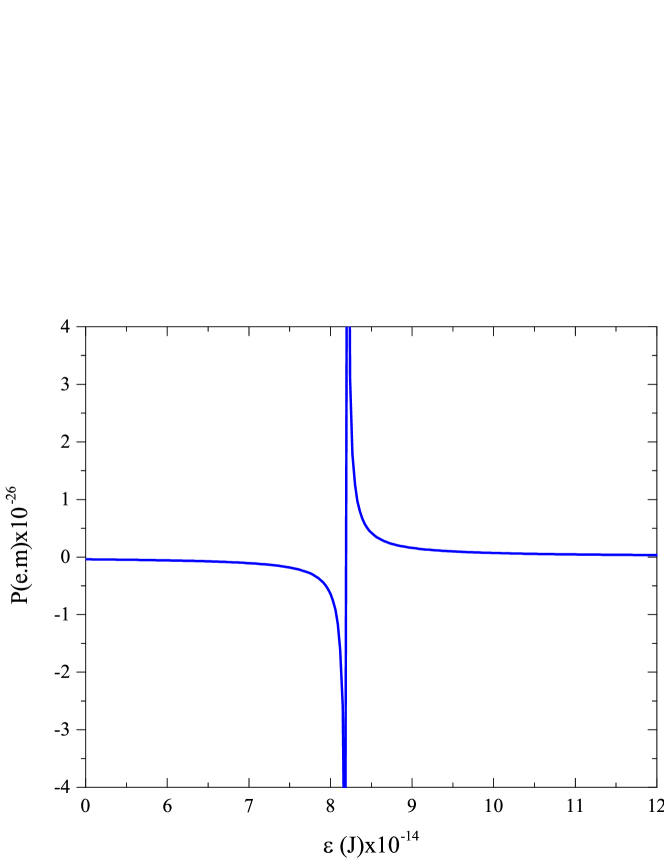
Figure 2: Calculated eEDMs under constant magnetic fields by using Eq.(15). In this calculation, by using $E-m_{e}c^{2}$, the kinetic energy and magnetic field values for the same transition and atom , respectively , $\varepsilon=[10^{-14},10^{-12.5}J]$ and $B=10^{-10}T$ .

In order to indicate the completeness of our approach and behaviour of eEDM, we first calculate the dipole moment by using the Eq.(15) under constant magnetic field for an electron being in a ¹³³Cs atom. For this calculation $6S_{1/2}\longrightarrow 6P_{3/2}$ transition and experimental values in Ref.[24] are used for kinetic energy of an electron and magnetic field. Here, we assume that electron has a kinetic energy of $\varepsilon=2.6\times 10^{5}eV$ and external magnetic field becomes in the range of $B_{0}=[0,4]\times 10^{-7}T$. Fig.1 shows that as the magnetic field strength increases, the eEDM slightly increases and does not change dramatically and it is also in the order of magnitude of $10^{-24}$ with unit of (e.cm). It is obviously seen that our calculation for above example is very close to previous findings[24].

Table 1: eEDM values for different magnetic fields and the kinetic energy values of an $e^{-}$ in ¹³³Cs atom.

$\varepsilon=(E-m_{e}c^{2})$	${B_{0}}$	$eEDM$
$(eV)$	$(G)$	$(e.cm)$
a)$\,10^{10}$	$[1,6]\times 10^{-3}$	$3\times 10^{-28}$
b)$\,10^{10}$	$[1,6]\times 10^{2}$	$9\times 10^{-26}$
c)$\,10^{5}$	$[1,6]\times 10^{3}$	$3\times 10^{-20}$
d)$\,10^{9}$	$[1,6]\times 10^{3}$	$3\times 10^{-24}$

We can also extend our calculations to different values of kinetic energy of an electron being in a ¹³³Cs atom and external magnetic fields for $6S_{1/2}\longrightarrow 6P_{3/2}$ transition. We first keep the $\varepsilon$ constant at $10^{10}$ eV while gradually increasing the $B_{0}$. Then, the $B_{0}$ is kept constant at $6.0\times 10^{-1}$ while increasing the $\varepsilon$. Using the values for $\varepsilon$ and $B_{0}$ given in Table I, we obtain the large number of values for eEDM as shown in third column of Table I.

Table 2: Comparison of our approach with previously published experimental studies.

$\varepsilon=(E-m_{e}c^{2})$	${B_{0}}$	$eEDM$ $in$ $this$ $work$	$Bound$ $for$ $\left|d_{e}\right|$
$(eV)$	$(G)$	$(e.cm)$	$(e.cm)$
$2.6\times 10^{5}$	$1.0\times 10^{-3}$	$3.1\times 10^{-24}$	$\left|d_{e}\right|\leq 7.7\times 10^{-22}$	[24]
$6.0\times 10^{6}$	$2.0\times 10^{-6}$	$5.9\times 10^{-27}$	$\left|d_{e}\right|$=$1.3\times 10^{-29}$	[25]
$1.0\times 10^{7}$	$2.55\times 10^{-2}$	$2.3\times 10^{-25}$	$\left|d_{e}\right|$=$(2.7\pm 8.3)\times 10^{-27}$	[26]
$1.0\times 10^{7}$	$7.0\times 10^{-3}$	$2.1\times 10^{-25}$	$\left|d_{e}\right|$=$4.0\times 10^{-27}$	[27]
$0.1\times 10^{7}$	$9.0\times 10^{-3}$	$2.0\times 10^{-25}$	$\left|d_{e}\right|\leq 1.6\times 10^{-27}$	[28]

In order to check the validity of our approach, we compare our calculations with previously published researches. In our all calculations, reported values for $B_{0}$, $\varepsilon$ and related transition for an atom are considered. For example, eEDM is, first, calculated for $B_{0}$ $=$ $2.0\times 10^{-10}T$ and $\varepsilon$ $=$ $6.0\times 10^{6}eV$, and it is obtained as $5.9\times 10^{-27}e.cm$ for $6^{2}S_{1/2}\longrightarrow 7^{2}P_{1/2}$ transition in ${}^{205}Tl$ atom. Secondly, we use $0.255\times 10^{-4}T$ and $1.0\times 10^{7}eV$ values for $B_{0}$ and $\varepsilon$, respectively. For $6^{2}P_{1/2}\longrightarrow 7^{2}S_{1/2}$ transition in ${}^{205}Tl$ atom, the eEDM’s magnitude is calculated as $2.3\times 10^{-25}e.cm$. Moreover, for $7.0\times 10^{-7}T$ of $B_{0}$ and $1.0\times 10^{7}eV$ of $\varepsilon$ values, the eEDM’s magnitude is found as $2.1\times 10^{-25}e.cm$ for $6P_{1/2}\longrightarrow 6P_{3/2}$ transition in ${}^{133}Cs$ atom. In our last calculation for $9.0\times 10^{-7}T$ of $B_{0}$ and $0.1\times 10^{7}eV$ of $\varepsilon$ for ${}^{205}Tl$ in its $6^{2}P_{1/2}$ ground state, the eEDM’s magnitude is obtained as $2.0\times 10^{-25}e.cm$. Our above calculations and previous findings are summarized in Table II. It can be clearly seen from the Table II that for each calculation we find eEDM values being very close to formerly reported values in the range of ignorable error.

Conclusion

In this study, we present an approach to compute the electrical and magnetic dipole moments of the electron by integrating the polarization and magnetization densities of the electron current on the hyper surface, respectively. The dipole moment expressions obtained by the approach are in compatible with the current experimental results. We also see that the magnetic field has an important effect on the electrical dipole moment of the electron: At first the eEDM increases with the square root of the magnetic field, $\sqrt{B_{0}}$, until it reaches to a maximum value for a certain value of the magnetic field, and then it decreases with $\frac{1}{\sqrt{B_{0}}}$. It is important to note that no matter how less its value gets it never reaches to the value (i.e. $10^{-38}$e.cm) predicted by the standard model, even if the magnitude of the magnetic field is in the Planck scale (i.e. the eEDM $\rightarrow 10^{-34}$e.cm as $B_{0}\rightarrow 10^{53}$T). From these results in the study, we clearly see that, in the case of $\varepsilon\ll\sqrt{2eB_{0}\hbar c}$, the magnetic field, $B_{0}$, squeezes or focuses the charge distribution of the electron.

References

- [1] B. L. Roberts and W.J. Marciano(eds)Lepton Dipole Moments (Advanced Series on Directions in High Energy Physics 20) (World Scientific),(2010).
- [2] P. Ošmera, I. Rukovanskı, Journal of Electrical Engineering, 59. NO 7/s, 74-77,( 2008).
- [3] M. Bezerra, W.J.M Kort-Kamp, M.V.Cougo-Pinto and C.Farina Eur. J. Phys. 33, No. 5, 1313-1320 (2012).
- [4] C. M. Sommerfield, Phys. Rev. 107, 328,(1957).
- [5] R. Arnowitt, B. Dutta, and Y. Santoso Phys. Rev. D 64, 113010,(2001).
- [6] C. Amsler et al. (Particle Data Group), PL B 667, 1 (2008) and(2009).(http://pdg.lbl.gov/).
- [7] J. Baron and et.all. Science 343,269-272,(2014).
- [8] B. C. Regan, Eugene D. Commins, Christian J. Schmidt, and David DeMille. Phys. Rev. Lett. 88, 071805 (2002).
- [9] D. F. Nelson, A. A. Schupp, R. W. Pidd, and H. R. Crane, Phys. Rev. Lett. 2, 492 (1959).
- [10] J.J., Hudson, D.M. Kara, I.J. Smallman, B.E. Sauer, M.R. Tarbutt, E.A. Hinds Nature 473 (7348), 493-496, 228, (2011).
- [11] D.M. Kara, I.J. Smallman, J.J. Hudson, B.E. Sauer, M.R. Tarbutt and E.A. Hinds, New J. Phys. 14, 103051 (32pp), (2012).
- [12] Y. J. Kim et al., Phys. Rev. D, 91, 102004, (2015).
- [13] B. Odom, D. Hanneke, B. D’Urso, and G. Gabrielse, Phys. Rev. Lett. 97, 030801 (2006).
- [14] A. N. Petrov, N. S. Mosyagin, T. A. Isaev, and A. V. Titov, Phys. Rev. A 76, 030501(R),(2007)
- [15] L. V. Skripnikov, A. N. Petrov, and A. V. Titov J. Chem. Phys. 139, 221103,(2013).
- [16] T. Ibrahim, A. Itani and P. Nath. Phys. Rev. D 90, 055006 (2014)
- [17] P. A. M. Dirac, Proc. R. Soc. (London) A117, 610 (1928), and A118, 351 (1928).
- [18] O. Stern, Phys. Rev. 51, 852-854 (1937).
- [19] J. L. Flowers, P. W. Franks, and B. W. Petley , IEEE transactions on instrumentation and measurement, V. 44, No. 2, April (1995).
- [20] Y. Sucu and N. Unal, J. Math. Phys. 48, 052503, (2007).
- [21] A. Jellal, A. D. Alhaidari, H. Bahlouli Phys.Rev.A 80:012109,(2009)
- [22] A. D. Alhaidari, H. Bahlouli, A. Jellal, Int. J. Geom. Methods Mod. Phys. 12: 1550062, (2015)
- [23] F. W. J. Olver, Asymptotics and special functions, Academic Press Network, p.207.(1974)
- [24] H. Ravi, U. Momeen, and V. Natarajan arXiv:1501.01624 [physics.atom-ph] ,(2015).
- [25] J. M. Amini, C. T. Munger, Jr. and H. Gould, Phys. Rev A 75, 063416,(2007).
- [26] K. Abdullah et al., Phys. Rev. Lett. 65, 2347 (1990).
- [27] Cheng Chin, Véronique Leiber, Vladan Vuletic, Andrew J. Kerman, and Steven Chu Phys. Rev. A,63(3):033401,(2001).
- [28] B. C. Regan, E. D. Commins, C. J. Schmidt and D. DeMille, Phys. Rev. Lett.88, 071805 (2002).
- [29] A. O. Barut and I. H. Duru, Phys. Rev. D 36, 3705 (1987).