Apse-alignment in narrow-eccentric ringlets and its implications for the -ring of Uranus and the ring system of (10199) Chariklo
Abstract
The discovery of ring systems around objects of the outer Solar System provides a strong motivation to apply theoretical models in order to better estimate their physical and orbital parameters, which can constrain scenarios for their origin.
We review the criterion for maintaining apse-alignment across a ring and the balance between the energy input rate provided by a close by satellite and the internal dissipation rate occurring through ring particle collisions that is required to maintain ring eccentricity, as derived from the equations of motion governing the Lagrangian-displacements of the ring-particle orbits. We use the case of the -ring of Uranus, to calibrate our theoretical discussion and illustrate the basic dynamics governing these types of ring.
In the case of the ring system of (10199) Chariklo, where the evidence that the rings are eccentric is not conclusive, we apply the theory of apse-alignment to derive information about the most plausible combination of values of the surface density and eccentricity-gradient, as well as the masses and locations of their postulated but -presently undetected- shepherd-satellites.
When the balance conditions that we predict are applied to the ring system of (10199) Chariklo, we are able to estimate the minimum mass of a shepherd satellite required to prevent eccentricity decay, as a function of its orbital location, for two different models of dissipation. We conclude that the satellite mass required to maintain the eccentric mode in the ring, would be similar or smaller than that needed to confine the rings radially.
Our estimation of the most plausible combinations of eccentricity gradient and surface density consistent with apse-alignment are based on a standard model for the radial form of the surface density distribution, which approximately agrees with the optical depth profile derived by the stellar occultations. We find a diverse range of solutions, with combinations of eccentricity gradient and surface mass density that tend to minimize required enhanced collisional effects, having adopted estimated values of the form factor of the second degree harmonic of the gravitational potential.
keywords:
Planetary, rings , Centaurs , Uranus rings , Resonances, rings , Planet-disk interactions1 Introduction
The discovery of the ring system around the Centaur (10199) Chariklo (Braga-Ribas et al., 2014, hereafter BR14) , the trans-Neptunian object (136108) Haumea (Ortiz et al., 2017) and the evidence that (2060) Chiron (Ortiz et al., 2015) is also surrounded by rings, poses an interesting theoretical challenge, not only to explain the origin of these unexpected features, but also to estimate better their physical and orbital parameters.
The surface density and the orbital frequency of the ring particles make the Centaur’s rings remarkable analogs of the narrow rings of Uranus or the outer rings of Saturn (BR14), However, it is not apparent that the same formation mechanism has occurred in all cases.
A number of scenarios have been put forward to explain the origin the rings, i.e., cometary-like activity (Pan and Wu, 2016), disruption of an asteroidal body through a close encounter with a major planet (Hyodo et al., 2016), ejecta produced in a physical collision either on the surface of the Centaur or with a conveniently located satellite (Melita et al., 2017) and the disaggregation of a satellite caused by the Centaur’s tidal field (Melita et al., 2017). In any case, it is apparent that a more precise estimation of basic physical and/or orbital parameters than is currently available would be helpful in deciding between different formation scenarios.
It has been shown that the rings of (10199) Chariklo are stable under close encounters with the major planets (Araujo et al., 2016). On the other hand, their migration timescale induced by the Poynting-Robertson effect is approximately and the spreading time scale arising from energy loss through inelastic collisions that result in an effective viscosity is only about (BR14). These short time scales indicate that the rings are being confined in their present location. A general argument can be made that such confinement requires the injection of energy with zero net angular momentum that is most likely supplied by non axisymmetric forcing (eg. Longaretti, 2017) which could originate from shepherd satellites. However, although this is viable in the case of the ring of Uranus no such shepherds have been identified for the and rings (but note Chancia and Hedman, 2016, who suggest that they may be below the limits of detection) and many other ringlets around Saturn. Such satellites could also account for the maintenance of ring eccentricity. In this situation it is natural that other phenomena have been suggested as providing required forcing. These include normal oscillation modes of the planet in the case of the Maxwell ringlet (French et al., 2016) and non axisymmetric variations of the B ring in the case of ringlets in the Cassini division (Hedman et al., 2010).
Thus the rings of (10199) Chariklo may be confined by shepherd satellites, estimated to have a physical radius of about with an assumed bulk-density of . We shall assume that such a satellite may also act to maintain ring eccentricity, however we note that the issue of the maintenance of uniform apsidal precession discussed below does not require this and would operate if some other phenomena provided an equivalent ring forcing.
Continuous observations of stellar occultations by (10199) Chariklo should enable us to better constrain the geometry of the ring system. At the present time, available observations are still compatible with a circular shape, with more being needed to establish its eccentric nature (Bérard et al., 2017). Nonetheless, the similarity between the asteroidal ringlets and the eccentric ringlets of the planets Saturn and Uranus indicates that the ones surrounding Centaurs may also be eccentric. In that case the orbits of the ring-particles must have their peri-apses alined and be precessing uniformly. A fact that makes it plausible that one of the centaur’s rings posesses a non-neglibile eccentricity is that the spin-orbit 1:3 second order resonance between the mean orbital frequency in a circular orbit and the intrinsic rotation frequency of (10199) Chariklo that could be manifested through a mass anomaly on it or within it rather than a 2:6 fourth-order resonance resulting from its ellipsoidal shape is close to or within the innermost edge of the ring system. These higher order resonances could play a relevant role in maintaining the eccentricity of the rings as well as providing energy and angular momentum input to counteract orbital decay resulting from collisional dissipation in a similar manner to shepherd satellites (see Sicardy et al., 2019) .
The precession of a ring particle orbit is induced by the oblateness of the primary with the angular velocity of the apsidal line being given, in the limit of very small eccentricity by (Murray and Dermott, 2000) as
where is the longitude of periastron and its time derivative, the physical radius of the primary is , its mass being , the form-factor of the second degree harmonic of its gravitational potential is , is the mean-distance between the particle and the primary, , and is the gravitational constant. Since decreases with increasing values of , in a ring system that is precessing uniformly, the differential precession that would be induced by the oblateness of the primary, if it alone acted, must be somehow compensated.
The leading model that accounts for uniform precession in narrow eccentric ringlets is the ”self-gravity model” (Goldreich and Tremaine, 1979), since precession induced by the self-gravity of the ring opposes that induced by the oblateness of the primary. A signature of narrow rings dominated by self gravity is that the eccentricity gradient, with being the semi-major axis, is a positive quantity such that the orbits of the inner ring particles are less eccentric than the outer ones (see (Papaloizou and Melita, 2005, hereafter PM05). Several ringlets in the Solar System are known to exhibit this type of behavior, for example the Titan and Maxwell rings of Saturn (Porco et al., 1984), and the , and rings of Uranus (Elliot et al., 1977). However, Goldreich and Porco (1987) find that, a model which balances differential precession induced by the central object with effects due to self-gravity, produces mass estimates for the , rings that are too low to be consistent with the possibility of confinement by perturbing satellites as well as high measured band radio opacities. These indicate that the masses are much larger, leading to the possible presence of collisional effects that counter the effects of increased self-gravity, as we indicate below ( see also Longaretti (2017) for further discussion). Collisional interactions such as those associated with close packing arising from converging streamlines and perturbations due to any shepherd satellites should be taken into account (Borderies et al., 1983; Mosqueira and Estrada, 2002; Chiang and Goldreich, 2000). We remark that the importance of the fact that the particles are close-packed at pericenter for the dynamics was recognised at an early stage (Dermott and Murray, 1980).
Here, we review a theoretical model of narrow-eccentric ringlets that has been applied to the rings of Uranus and the Titan-ringlet of Saturn (PM05 and Melita and Papaloizou, 2005, respectively) Our aim is to investigate how ring eccentricity is maintained against collisional dissipation and different processes are able to contribute to the maintenance of uniform precession. We consider the importance of significant collisional interactions resulting from phenomena such as close packing, intersecting streamlines and torquing from external satellites together with the associated energy loss. In addition we relate this to shepherd satellites postulated to be needed to counteract ring spreading and orbital decay.
When applied to the case of the ring system of (10199) Chariklo, this discussion leads to constraints on the masses and orbits of putative shepherd satellites, the mass density of the rings and collisional interactions that occur between ring particles.
In section 2 we review the latest estimates of the physical and dynamical properties of (10199) Chariklo and its rings. In section 3 we review the apse-alignment theory, deriving the conditions to maintain a non-zero mean eccentricity and the apse-alignment of the ring particle orbits.
We apply the radial-action balance equation to estimate the mass of the shepherd satellites responsible for maintaining the eccentricity in section 4. In section 5 we validate the equation that expresses the balance of impulses to achieve the apse alignment for the case of the -ring of Uranus and apply it to the ringlets of (10199) Chariklo. In the last section we discuss our results and draw some conclusions.
2 (10199) Chariklo and its ring system
The main orbital and physical properties of Centaur (10199) Chariklo are summarized in table 1. Its orbit is fully contained between the orbits of Saturn and Uranus, with moderate values of eccentricity and inclination. It is known that the Centaur population exhibits a bimodal distribution of surface colour indexes (Peixinho et al., 2003) and (10199) Chariklo belongs to the “grey” or “neutral” group (as opposed to the “red” group), which might be associated with the existence of cometary-like activity in the past (Melita and Licandro, 2012).
| Absolute magnitude(1) | |
|---|---|
| Apparent magnitude(1) (V) | |
| Colour index(1) () | |
| Orbital semimajor axis(1) | AU |
| Orbital eccentricity(1) | |
| Orbital inclination(1) | deg |
| Physical radius (Jacobi)(2) R1J | () km |
| Physical radius (Jacobi)(2) R2J | () km |
| Physical radius (Jacobi)(2) R3J | () km |
| Bulk Density (Jacobi)(2), | |
| Albedo (Jacobi)(2), | |
| Mass (Jacobi)(2) | g |
| Sidereal intrinsic rotation period(2) | () hr |
In Table 1 we only quote the estimate of the shape of the body of (10199) Chariklo made assuming it to be a Jacobi ellipsoid, noting that those made assuming an arbitrary triaxial ellipsoid are similar. We note that, according to the most recent reference (Leiva et al., 2017), the oblateness is remarkably large, . Based on the oblateness of the body, the form factor of the second degree harmonic of the gravitational potential, can be approximated as
(Pan and Wu, 2016). On the other hand if it is assumed that the shape of the body is given by the equipotential surface determined by the self-gravity and the centrifugal potential, the form factor of the second degree harmonic of the gravitational potential is given by
with being the intrinsic rotational frequency, the gravitational constant, is the physical mean radius of the body and its mass (Murray and Dermott, 2000). We find that if it is assumed that (10199) Chariklo is a Jacobi ellipsoid, then and , whereas if an arbitrary ellipsoidal shape is assumed, and . It must be noted that these estimations of are about two orders of magnitude larger than the typical value for a major planet in the Solar System and also that the early estimate, made assuming that the values of the radii of the body are those given in BR14, render a smaller value of (see also Pan and Wu, 2016).
The discovery of a ring system consisting of two dense ringlets separated by a gap was made through the observation of multi-chord stellar occultations (BR14). The two ringlets are known as “CR1” and “CR2”. A recent update on the physical properties of the (10199) Chariklo ring system has been reported by Bérard et al. (2017) (B17) where it is argued that some of the properties of the CR1 ringlet (shaped profile, variation of width with longitude and sharp edges) make it quite similar to those of the narrow eccentric ringlets of Saturn (Nicholson et al., 2014; French et al., 2016) or Uranus (Elliot et al., 1984; French et al., 1986) .
In Table 2 we summarize some of the ring properties reported in B17. It has been estimated that the total eccentricity variation across the ring, may be of the order of with denoting the width variation, which we also asssume equal to the lower limit of the eccentricity at the inner edge. However, the most statistically significant model of the ring, performed using the latest data available at present is compatible with a circular ring.
In summary, for our current purposes we shall assume an inner eccentricity, , with a constant eccentricity gradient that is compatible with an eccentricity variation of , as estimated in B17. To obtain a more accurate estimation of the geometry in the future, the degeneracy between the ring eccentricity and the position of its pole has to be lifted, which should occur with the accumulation of future observations of stellar occultation events.
| CR1 ringlet radius, rCR1 | 390.6 |
|---|---|
| CR2 ringlet radius, rCR2 | 405.4 |
| Optical Depth of the CR1 ringlet, | |
| Optical Depth of the CR2 ringlet, | |
| Width of the CR1 ringlet, | () |
| Width of the CR2 ringlet, | () |
| Width variation of the CR1 ringlet, | |
| Width of the gap, | |
| Sharpness of the CR1 ringlet, | |
| Optical Depth in the gap, | |
| Mean orbital Period of the rings, | |
| Mean orbital frequency, | |
| Mean precession frequency, | |
| Mean precession frequency, |
Relevant evolutionary timescales for the system are estimated to be very short with respect to the dynamical age of a typical Centaur. The timescale in which the rings would spread a distance equivalent to its orbital location by the Poynting-Robertson effect is estimated by BR14 to be , T and through viscous dissipation, assuming the ring to be a monolayer, to be, T where is the particle size in metres. The maximum survival time against orbital dislocation occurs for and is This time will be significantly less for significantly larger or smaller particles. Hence the existence of shepherd satellites that provide confinement is implied, as otherwise the system would have a remarkably unlikely short age. The physical radius of a shepherd satellite capable of producing an adequate shepherding effect, was estimated to be about for a bulk density of . While the physical radius of a body capable of clearing the observed gap between the CR1 and CR2 ringlets is , for a bulk-density of (see BR14).
3 The dynamics of apse-alignment and eccentricity maintenance
The goal of the theoretical modelling of the ringlets is to explain quantitatively how the eccentricity is sustained against collisional dissipation and how the different forces acting are balanced to produce rigid precession. In PM05 the rings were modelled as a two dimensional continuum adopting a Lagrangian description. The equations of motion are developed for perturbations with respect to a background state in which ring particles are in circular orbits and are characterised by the associated Lagrangian displacement.
In the axisymmetric unperturbed state, particles are in circular motion, such that
Here we adopt a cylindrical coordinate system with origin at the central mass, . Thus the value of, for the circular orbit of a given particle in the background state is is its angular velocity and is a phase factor. From now on a subscript, denotes application to the background state. The components of the Lagrangian displacement from the axisymmetric background state are given by These are such that the perturbed coordinates of a perturbed particle are given by
| (1) |
and
| (2) |
The Lagrangian variation of given quantity , is defined as
| (3) |
where and are the values of the given physical quantity in the perturbed and unperturbed flow respectively. It thus represents the variation as experienced by a fluid element at original location In contrast, the Eulerian variation, measured at a fixed location, is defined as
| (4) |
Thus to first order in the operators, and are related by
| (5) |
and we note that and
The components of the equation of motion we use are given by (see PM05)
| (6) |
| (7) |
where is potential due to the central mass and where is the sum of the potentials related to the satellites, and the self-gravity of the ring, , are the variations of the components of the force per unit mass due to particle interactions. These could be associated with dissipative collisions and/or as indicated by Chiang and Goldreich (2000) an effective pressure. In writing equations (6) and (7) we neglect background self-gravity on account of the small mass of the ring.
We comment that in this section we adopt the time averaged figure of the central object. Thus we do not consider harmonically varying gravitational forces resulting from the non axisymmetric shape. Such effects can act in a similar manner and be treated with the same formalism applicable the perturbations from a shepherd satellite discussed in Section 3.6
We further remark that denotes the Lagrangian time derivative on a fixed particle. In addition the perturbing satellites are not included in the background state but are introduced as perturbing quantities which act on the particles at their perturbed position. Thus
| (8) |
The second term on the right hand side of (8) is accordingly of second or higher order in perturbed quantities and would be omitted in a strictly linear analysis. On the other hand in working with the left hand sides of equations (6) and (7) we make the epicyclic approximation and accordingly retain only terms of first order in the perturbations. In addition we have
3.1 The condition for rigid-precession
We here consider the situation when the perturbation takes form of an mode which forms a steady pattern in an appropriate rotating frame. This corresponds to the ring being eccentric and precessing uniformly. The frame in which the pattern is stationary rotates with the precession frequency
To obtain a condition for this to hold, we rewrite equation (6) as
| (9) |
where the quantity is defined by
| (10) |
and the square of the epicyclic frequency is given by
| (11) |
We note that the local precession frequency of a free particle orbit is
Following (Shu et al., 1985), we transform to the coordinate system rotating with the pattern frequency In this frame the azimuthal angle in the background state becomes We look for steady solutions in this frame which depend only on and In this case in equations (6) - (9) we have
| (12) |
Making use of this, after straightforward algebra, we obtain the following relation from these equations
| (13) |
where:
| (14) |
is the integrated radial component contribution of the collisional interaction,
| (15) |
is the integrated azimuthal component contribution of the collisional interaction, and
| (16) |
gives the contribution form the self-gravity of the ring, where we are assuming that there are no satellites that contribute directly to the form of the wave mode.
Assuming that the eccentricity is small, so that we may adopt the epicyclic approximation, for which the radial displacement takes the harmonic form on integrating over equation (13) gives
| (17) |
By using the approximation and , equation (17) can be written
| (18) |
where
Equation (18) has to be satisfied to enable rigid precession of the ring. When external satellites are absent, the latter occurs when contributions from self gravity and collisions on the right-hand side balance the differential precession term on the left-hand side.
3.2 The self-gravity term
For the computation of we also follow S85. The local self-gravity at is canonically assumed to be that of a band of thickness , where and are the inner and outer limits of the unperturbed ring respectively. In addition we assume the radial scales in the problem are much smaller than the angular scales so that the component of the force due to self-gravity may be neglected. This is the tight winding approximation. Thus we write (PM05)
| (19) |
where is the gravitational constant, and is the mean radius of the background ring. We set and , where we recall and . We remark that the background potential due to self-gravity is included in (19). However, this is inconsequential as it has been considered negligible. In addition principal values of the integrals are to be taken.
In the tight-winding approximation the conservation of mass of a moving fluid element requires that
| (20) |
Thus we have
| (21) |
We can re-write equation (21) in terms of the parameter, with
| (22) |
Then we find
| (23) |
can be expressed as
| (24) |
where:
| (25) |
Note that the integral in equation (24) being dealt with the principal value prescription requires to vanish smoothly at edges in order to avoid a singularity. It can be particularly complicated to evaluate in practice.
3.3 The pattern frequency
If we multiply both sides of Eq. ((18)) by and integrate radially across the ring, assuming that, consistently with the conservation of momentum and angular momentum, the integrated collisional terms vanish, we obtain:
| (26) |
In addition the integral on the right hand side can readily be seen to vanish identically, therefore we can calculate the value of the pattern frequency, , as:
| (27) |
We remark that for a thin ring can be approximated as being constant in the above integrals and thus may be cancelled out.
3.4 The value of q
In the linear regime: , , so then multiplying both sides of Eq. ((24)) by and integrating radially across the ring we obtain
| (28) |
On the other hand, from Eq. (18) we can write:
| (29) |
Thus, if the effect of collisions can be neglected in comparison to that due to self-gravity, it is verified that:
| (30) |
We remark that in the linear regime the pattern speed, may be regarded as an eigenvalue associated with a normal mode determined by Eq. (18). For a mode which is such that does not change sign, as in the case of interest here, it follows directly from equation (27) that must equal the local precession frequency, at some intermediate point in the ring, with radius say, thus . Thus with the help of (27) and (30) , we can verify that
| (31) |
which with the use of the intermediate value theorem can be written as
| (32) |
where is a value of intermediate between and
For a thin ring we may perform a first order Taylor expansion and set where the derivative is evaluated at Inspection of the integrand in (32) implies that if and do not change sign we must have
| (33) |
As the precession frequency decreases outwards, the eccentricity gradient is necessarily positive in any thin ring where self-gravity is the main mechanism that maintains apse alignment and the gradient does not change sign (see also Goldreich & Tremaine 1979, Borderies et al. 1983).
To estimate the value of in a narrow-eccentric ring, in the linear regime where , when all perturbations other than self-gravity are neglected, we begin by noting that from Eq. (18), we can estimate
| (34) |
Here for some quantity estimates its variation across the ring, thus gives the magnitude of the difference between the free particle precession frequencies at the ring edges. Hence making the identification we find that
| (35) |
Hence, the magnitude of is related to the mass, size and eccentricity of the ring and the value of the second degree harmonic of the gravitational potential of the central object, .
3.5 Conservation of radial action
Following (PM05) we define
| (36) |
where the integral is taken radially and azimuthally over domain of the ring. For radial displacements of the form, as adopted above, for a slender ring this integral corresponds to the standard radial action, expanded to first order in Here the semi-major axis,
An expression for a conservation law for the radial action associated with the mode can be found by finding an expression for the time derivative of Eq. (36) as was done in (PM05). To do this we return to the inertial frame and adopt and as independent variables while retaining the possibility of general time dependence that is assumed to be slow as compared to the orbital time scale. Thus we write
| (37) |
and we recall that in linear theory, can be replaced by the unperturbed value. Also we have
| (38) |
The assumption of slow evolution enables us to neglect the first term in the above and the assumption of an harmonic dependence on, then allows us to write
| (39) |
Using the above Equation (9) take the form
| (40) |
On multiplying (40) by and integrating over the mass of the ring, after performing an integration by parts and with the help of Equation (7) we obtain
| (41) |
We remark that in obtaining Equation (41) we have neglected the time derivative of when making use of Equation (7) and finally used the relation which applies to free epicyclic motion in order to obtain this term in the second integral on the right hand side.
For a ring in which a steady eccentricity is maintained, noting that there is no net contribution from the ring’s self-gravity (the terms involving ), the secular rate of change of due to satellite forcing must balance that due to the effect of collisions acting on the perturbation. From (41) this is seen to be equal to the ratio of the rate of energy dissipation associated with them that is induced by the perturbation to the local orbital frequency. In such a case that is the condition that on average, remains constant.
As there is no net contribution from self-gravity when integrated over the mass of the ring, any dissipation arising from internal friction can only be compensated by the action of external forces that produce satellite torques. The exact multiple of a satellite torque that acts on the ring so as to maintain the mode against energy dissipation is considered in the next Sections.
3.6 Resonant satellite torques
Consider a satellite in circular orbit with angular velocity . We suppose that there is a second order Lindblad resonance at some point in the ring where
| (42) |
for azimuthal mode number, The upper/lower signs respectively corresponding to an interior/exterior satellite. Note that this condition is expressed in terms of the orbital rotation frequencies as seen in a frame rotating with the ring precession frequency. If we neglect orbital precession by setting and this gives the condition
For large this corresponds to the satellite being a distance from the nearest ring edge. If is large, as we shall assume, the satellite may have both first and second order Lindblad resonances within the ring. The first order resonances may be associated with ring confinement, leading to a shepherding role for the satellite, the second order resonances being associated with eccentricity driving. In order for there to be a second order resonance but no first order resonance the ring must be sufficiently thin, such that When the situation is marginal a single satellite may have a first order resonance at the ring edge providing confinement together with second order resonances at the edge and in the ring interior which can drive eccentricity.
Returning to the case of a second order resonance expressed by (42) the contribution of the terms involving a satellite potential in the integrals on the right-hand side of Eq. (41) are directly related to the resonant torque generated by the forcing between the satellite and ring as occurs in Eq.’s (6) and (7) through its contribution to the forcing gradient of potential (see PM05).
The forcing amplitude is proportional to both the satellite potential and the ring eccentricity. We neglect additional forcing terms that can arise from the components of with azimuthal mode number , and we assume that the ring-satellite torque is then produced by the direct forcing of the unperturbed background ring a procedure that is assumed adequate to provide the total torque.
The total torque, induced by a satellite on the eccentric ring can be estimated as in Goldreich & Tremaine (1978). An expression within the framework of the Lagrangian displacement is given in PM05. If the resonance occurs with ring material with angular velocity the disk is forced by a disturbance with a definite pattern speed, and the rate of change of ring orbital energy is related to the rate of change of ring angular momentum by
| (43) |
which expresses the well known result that the ratio of energy to angular momentum exchanged is (see also Friedman and Schutz, 1978) . We also have the contribution to given by
| (44) |
Note that is respectively positive/negative for an interior/exterior satellite so that the contribution to is always positive resulting in ring eccentricity growth. Of course the contributions from all satellites and relevant resonances must be incorporated. These positive contributions to have to be balanced by effects due to collisions.
3.7 Estimate of the magnitude of an eccentricity driving satellite torque
We use the balance Equation (41) to estimate the masses of the putative shepherd satellites of (10199) Chariklo’s ring system as a function of their location with respect to the ring. Since here we are only interested in an order-of-magnitude estimation, we shall only consider an interior satellite in a circular orbit with an associated exterior second order resonance. The corresponding calculation for an exterior satellite with an inner resonance is entirely analogous.
We estimate the satellite torque resulting from the forcing described in Section 3.6 from results of (Goldreich and Porco, 1987) who give
| (45) |
where we recall that is the mean distance from the ring to the central body, is the unperturbed surface density of the ring, the eccentricity of the ring, and here being evaluated at the location of the resonance, is the mass of the perturbing satellite and the mass of the central body. The contribution to the rate of change of radial action may then be found from (44) with the choice of upper sign.
4 The energy dissipation rate in an asteroidal ring and the masses of perturbing satellites
To estimate the energy dissipated per unit mass in the ring, we envisage that local velocity differences which might arise from streamline intersection produced by differential precession or from the action of external satellite torques, are counteracted by forces that arise through collisions. It has been suggested that these could occur as a consequence of close-packing that ring-particles experience when they go through pericenter (Dermott and Murray, 1980) or an increased velocity dispersion produced through the ring satellite interaction (Chiang and Goldreich, 2000). In order to estimate the rate of energy loss due to these effects we adopt the following heuristic approach. We introduce a velocity scale through where is the difference between the precession frequency induced by the oblateness of the central object at the edges and is the eccentricity. This is roughly the radial velocity difference between the edges at pericentre that is induced by differential precession on an orbital time scale after initial alinemment.
We write the energy dissipation rate as, , where: (see also PM05)
| (46) |
where we recall that is the width of the ring and , a scaling factor which in addition to scaling the velocity could include effects of inelasticity through a restitution coefficient. We remark that the above rough estimate, with of order unity, is expected to be of the correct order of magnitude if gives the correct velocity scale for dissipation on an orbital time scale. We remark that the postulated enhanced collisional effects that may occur very close to sharp edges (Chiang and Goldreich, 2000) may be incorporated through an appropriate choice of
In the case of the -ring of Uranus, it has been shown that, when collisional effects, as estimated above, with , are assumed as the main cause of dissipation that is balanced by the rate of increase of the ring radial action driven by a perturbing satellite, Eq. (44) together with (45) yields excellent agreement with the required ratio of energy input rate to angular velocity found from (46) when the mass and orbit of the shepherd satellite Cordelia (PM05) are adopted.
4.1 Viscous dissipation in the background flow
However, apart from effects arising from a non zero eccentricity, there is a rate of energy dissipation associated with an effective viscosity acting on the background Keplerian flow, , which is given by (Lynden-Bell and Pringle, 1974)
| (47) |
where is the mass of the ring. In order to make the estimates below we evaluate and at the resonance radius Thus and In addition we estimate the local magnitude of the kinematic viscosity as , where is the associated semi-thickness with being the ring density at
We suppose that eccentricity driving occurs through the operation of a second order resonance with a single interior satellite and this is balanced by energy dissipation through impulsive collisions for the most part near the ring edges. This implies that the satellite radial action input rate given by Eq. (44) obtained with the help of (45) balances with the ratio of the energy dissipation rate to angular velocity found from (46). This condition enables the mass of the satellite to be expressed in units of the mass of the central object as
| (48) |
For comparison we give the satellite mass under the assumption that the rate of increase of radial action induced by the satellite is balanced by the ratio of the background dissipation rate to angular velocity in the form
| (49) |
This will exceed when the background viscous dissipation exceeds that arising from enhanced collisions arising from satellite perturbations and close packing. It is important to note that this is not a condition for the satellite torques to prevent viscous spreading. In that case the satellite torque must balance the viscous outward angular momentum flow rate (Goldreich and Tremaine, 1978, e.g.)
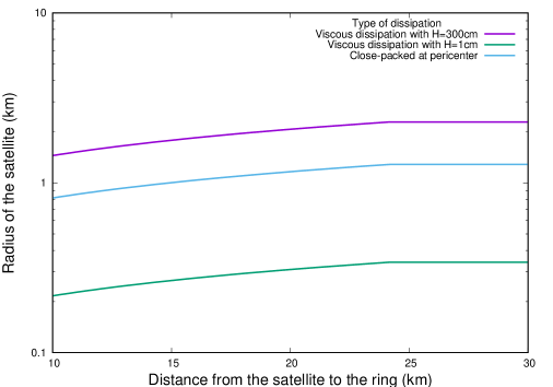
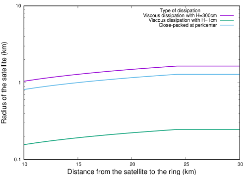
In Fig. 1 we plot radius estimates for an interior perturbing satellite of (10199) Chariklo’s ring system, as a function of the distance from the satellite to the ring, which can be approximated as
| (50) |
which in turn can be used to express in terms of in the form
| (51) |
The parameters of the ring system used to produce the plots are given Section 2. The satellite resonance and enhanced collisions are assumed to be in the CR1 ringlet with . Two values of the eccentricity of the ringlet have been adopted in equation (46) when evaluating the energy dissipation rate as a result of satellite forcing and/or close packing, for the calculation displayed in the upper panel and for the calculation displayed in the lower panel. The energy dissipation rate due to viscosity was evaluated for the semi-thicknesses, and respectively corresponding to estimated values of , for an assumed The differential precession rate across the ring, was taken to be , which corresponds to a value of and the location and width of the CR1 ringlet were adopted. Note that in the case where dissipation arises through satellite forcing and/or close packing, the estimated radius of a satellite necessary to counteract the decay is between and smaller than the values plotted in Fig. 1 for assumed values of between and , and then its size is smaller than that of a satellite needed to achieve confinement (BR14). The energy produced by viscous dissipation is significantly larger than that arising through enhanced collisional effects when the assumed surface density is and it is similar when the assumed surface densty is .
We may also estimate the potential importance of the 1:3 second order resonance between the mean orbital frequency in a circular orbit and the intrinsic rotation frequency of (10199) Chariklo. This is close to the inner edge of CR1 and could act to balance dissipative collisional effects arising from close packing were this resonance to be inside the ring. Sicardy et al. (2019) estimate that the non spherical deformation of (10199) Chariklo could amount to a mass anomaly of This corresponds to an object of radius which is about a factor of two larger than the radii indicated in Fig.1. However, the object has to be regarded as more than an order of magnitude further away. The corresponding value of whereas for objects indicated in Fig.1, Use of equation (45) for this virtual mass indicates that if the resonance is indeed inside the ring the torque input is about an order of magnitude smaller than for those considered in Fig. 1. However, significant effects could arise if the mass anomaly was three times larger than that assumed. In that case it could act together with closer satellites to maintain the ring eccentricity.
5 The condition of apse-alignment across the ring and the surface density
5.1 Probing the model of apse-alignment for case of the -ring of Uranus
On the left hand side of Eq. (18) we have the product of the local rate of differential precession relative to an assumed precession of the ring as a whole and its local radial displacement, the latter being the product of the local radius and eccentricity. On the right hand side of Eq. (18) we find contributions from the agents that can balance this and enable the entire ring to undergo uniform precession, i.e. ring self-gravity and inter-particle interactions.
For the cases treated here there is no satellite with an orbit such that its orbital frequency is resonant with the pattern precession of the ring, as in the case of the “Titan” ringlet of Saturn that was considered in Melita and Papaloizou (2005). Accordingly, to calibrate the model we will apply it to the -ring of Uranus, where independent estimates of the eccentricity, the eccentricity-gradient across the ring and the surface density can be made from Voyager 2 PPS Persei and Sagittarii stellar occultation measurements (Graps et al., 1995).
Our goal is to verify that the independent estimate of the value of the surface density leads to contributions from self-gravity that can potentially counteract the differential precession induced by the oblateness of Uranus, across the ring. In addition we compute the contribution from inter-particle forces in those locations where the contribution from ring self-gravity is unable to exactly match that required to balance the kinematic rate of differential precession.
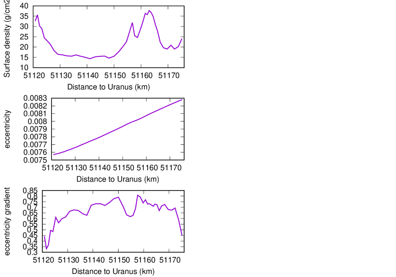
The input data from the -ring, (Graps et al., 1995), is shown in Fig. 2. The surface density profile, , was estimated from the optical-depth profile from , where is the mean density of the individual particles in the ring, and is their radius. If we assume that and we obtain an approximate mean value of (Fig. 2). Unfortunately, there is not enough data to produce an accurate average of the surface density over all azimuthal angles. The input data that we use is obtained from an average of four different stellar occultation events. Some azimuthal structure may not be canceled properly by our averaging procedure, which may explain some of the radial variation seen in the plot. Notice also that the eccentricity gradient is remarkably constant across the ring, i.e. to a high degree of accuracy the eccentricity increases linearly from one edge to the other.
In the Appendix we show how the self-gravity contribution, is computed from the discrete data. This data, (Graps et al., 1995), contains information from different locations across the ring, which were re-sampled to obtain a total number of on a suitable equally spaced grid, since the limit set in the Appendix to comply with the sampling theorem is about . This corresponds to a radial resolution of We recall that the edges of the ring are not resolved observationally or by the theoretical model at this level.
The azimuthally integrated inter-particle collisional contribution, is readily obtained from Eq. (18) as:
| (52) |
We compute from the available data as
The quantity, is assumed to be constant. To justify this we begin by noting that From the data plotted in Figure 3 below, we see that neglecting a fractional errors of order the the ring width to radius ratio, the second term may be neglected and an approximately linear variation of eccentricity implies that is approximately constant. In this way, becomes equivalent to the eccentricity gradient introduced in Section 1, being a situation that applies to thin rings in general and we may write
| (53) |
The precession frequency is given by
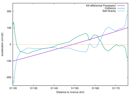
where and are the second harmonic of the gravitational potential and the physical radius of Uranus respectively. In Figure 3 we plot as a function of radial location in the ring, the acceleration needed to balance the differential precession due to the oblateness of Uranus, , with being given by equation (27). Notice that this quantity is positive in the inner edge and negative in the outer edge, because the precession rate decreases with distance. The acceleration due to self gravity and the component arising from particle interactions, , as obtained from Eq. (52 ) are also plotted. Their sum balances the effect of differential precession.
We note that close to the edges the collisional component is significant and contributes in the same sense as the component induced by the oblateness of the planet, while the self-gravity component that together they balance is opposed and larger in magnitude than each of them.
5.2 The ring system of (10199) Chariklo
Our goal is to estimate the most plausible values of the assumed constant eccentricity gradient and surface density for the CR1 and CR2 ringlets and, for that purpose we assume that the real values of these parameters are such that the integrated effect of collisions needed to balance effects due to differential precession are minimum values. We assume 2 possible extreme values of for (101999) Chariklo, , as taken from Leiva et al. (2017) assuming that the surface of the body is an equipotential determined by the combined effects of centrifugal forces and self gravity and as estimated by BR14 and Pan and Wu (2016).
We define the quantity, as
| (54) |
where and are the inner and the outer radial boundaries of the ringlet respectively and is the width of the ring. This quantity which we shall describe as an integrated collisional term is an integrated collisional acceleration orbital frequency.
5.3 The CR1 ringlet
For the CR1 ringlet we assume a mean distance from the Centaur of km and an eccentricity at the inner edge of . We compute the value of for assumed constant values of (see equation (53)) between and , which are compatible with the presently available observations. The upper bound of has been chosen to be similar to that found for the planetary eccentric ringlets.
The surface density profile is assumed to be constant between the inner and the outer edge, and we explore values that range between and . We note that the assumption of a uniform interior surface density qualitatively agrees with the observation of a uniform optical-depth profile (BR14 and B17). The top hat profile is justified on account of the sharpness of the rings being observed to be much smaller than the resolution of the occultation data (BR14 and B17). The resolution of the grid used for numerical modelling (see the Appendix) was approximately and so the edge is not resolved at smaller scales. We also assume that the eccentricity gradient is positive and constant across the ringlet and therefore, the eccentricity increases linearly between the inner and the outer edge.
The values of surface density, eccentricity gradient that minimize the collisional term are given in table 3 for both ringlets.
| CR1 | CR2 | |||||
|---|---|---|---|---|---|---|
| () | () | () | () | |||
| 10.0 | 0.21 | 7.90 | 10.0 | 0.06 | 2.16 | |
| 10.0 | 0.29 | 13.37 | 22.2 | 0.03 | 3.88 | |
| 10.0 | 0.01 | 7.45 | 10.0 | 0.01 | 0.86 | |
| 10.0 | 0.01 | 7.47 | 10.0 | 0.02 | 1.21 | |
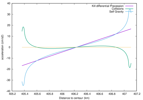
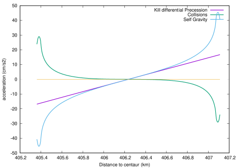
In the case in which the integrated collisional term, , for the CR1 ringlet is minimised for a value of , and a value of the surface density of . The radial distribution of accelerations for this case is illustrated in Figure 4. For the model in which the slopes of the self-gravity contribution and the differential precession contribution are equal at the middle of the ringlet removing the need of a significant contribution from the collisional term there, the overall dissipation is about twice as large as in the previous model for the same value of the surface density and a similar but larger value of eccentricity gradient. The corresponding radial distribution of accelerations is illustrated in Figure 5..
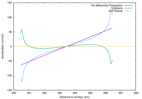
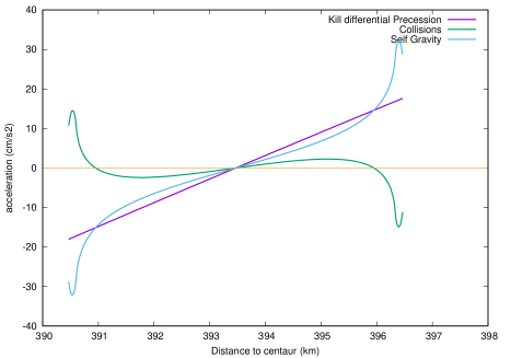
For a lower value of we find that the collisional acceleration is minimised for a smaller value of the eccentricity gradient, , and a value of surface density, , as in teh previous case. The radial distribution of accelerations for this case is illustrated in Figure 4. For , the model in which the self-gravity compensates the differential precession induced by the oblateness of the Centaur in the middle section of the ringlet occurs for a larger value of surface density, producing a slightly larger collisional term . The corresponding radial distribution of accelerations is illustrated in Figure 5.
For the models where the integrated collisional term is minimised and self-gravity approximately compensates the differential precession induced by the oblateness of the Centaur in the middle of the ringlet, the difference is noticeably larger at the edges, where, therefore, substantial collisional effects are needed there to produce a balance. This occurs because self gravity is significantly amplified at a sharp edge where it overcompensates for the effect of differential precession, requiring a significant enhancement of collisional effects to provide a balance.
The reason for the amplified effects of self gravity at an edge is that the tendency for gravitational effects due to interior material to cancel those arising from exterior material at any point in question is absent. This leads to an enhancement factor where is the characteristic scale associated with the edge, typically this factor for the models considered here.
On account of this it is of interest to highlight solutions for which the differential precession is exactly compensated for by self-gravity in the central region of the ringlet, but then even larger collisional contributions are implied in the regions close to the edges, an effect that is illustrated in Fig. 5, for both of the assumed values of .
5.3.1 The CR2 ringlet
We now apply the above analysis to the outer, narrower and fainter ringlet CR2. We assume a mean distance from (10199) Chariklo of and the same value of the inner eccentricity as for CR1. We also assume similar surface density profiles and constant values for the parameter , as in the case of the CR1 ringlet. The central uniform surface density values explored also range between and and as before, was taken to be in the range The resolution of the grid used for numerical modelling in this case was approximately
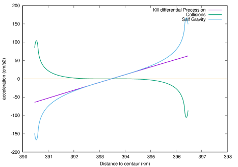
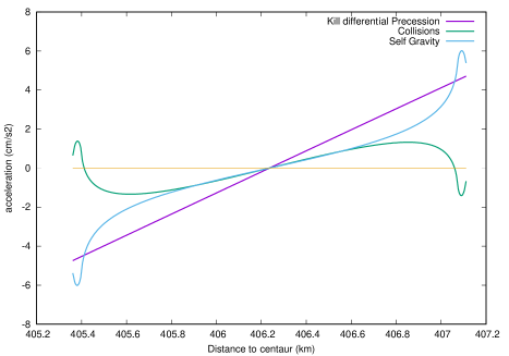
In the case of the CR2 ringlet the integrated collision term is minimised for much smaller values of the eccentricity gradient, giving for and for , with a value of the surface density in the first case equal to that for the corresponding CR1 case of As expected, the integrated collisional contribution is significantly smaller as compared to corresponding cases for the larger ringlet. The distributions of the accelerations for these cases are illustrated in Figure 6.
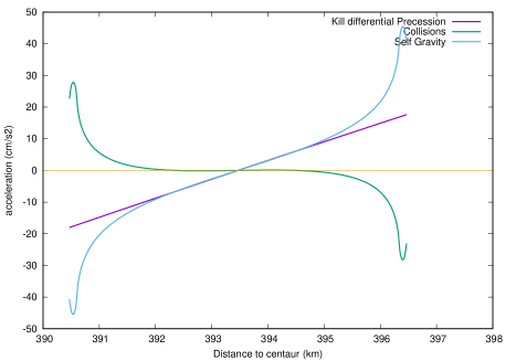
As for the CR1 case we determined models, that almost entirely remove the need for the collisional term in the middle section of the ring. The parameters are given in table 3 and the distributions of the accelerations are illustrated in Figure 7.
Qualitatively, the behaviour of the CR2 ringlet is similar that of the CR1 ringlet, i.e. the acceleration imparted by self-gravity approximately balances the differential precession, except at the edges, where the self-gravity is dominant and significant forces arising from collisions are needed to enable rigid precession there.
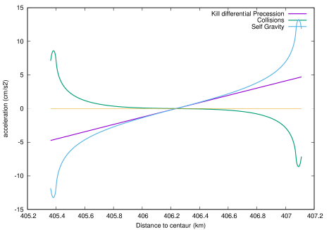
Having made the above calculations which indicate the necessity of important collisional effects near the edges if they are sharp, we remark that the CR2 ringlet is of low optical depth (see Table 2) making collisional effects due to enhanced packing potentially implausible. In this context we note that the edge profile is not constrained by the observations (B17) so that it could be more tapered than assumed, obviating the requirement for enhanced collisional effects. This may be a consequence of there being no external satellites driving ring eccentricity in this case.
6 Discussion and Conclusions
We have applied the theory of apse alignment in narrow eccentric ringlets as considered in (PM05) and discussed further in Section 3 to the ring system of (10199) Chariklo.
We considered the conditions for the maintenance of rigid body precession through the action of self-gravity and collisional effects counteracting the effect of differential apsidal precession in Sections 3.1-3.4 going on to consider the conservation of the ring radial action and the balance of collisional dissipation and ring satellite torques required to maintain the eccentricity in Sections 3.5-3.6.
A simple estimate for the collisional dissipation arising as a result of close packing possibly occurring in an eccentric ring at a pinch near pericentre (see Dermott and Murray, 1980) or through satellite ring interaction (Chiang and Goldreich, 2000) was given in Section 4. Focussing on parameters appropriate to the optically thicker and more extensive CR1 ringlet, and using this estimate, we showed in Section 4.1 that the mass of the satellites needed to prevent eccentricity decay associated with the mode, for which the ringlet precesses uniformly, are estimated to be similar to those needed to produce confinement against viscous spreading as estimated in BR14.
In order to validate our procedures we applied the rigid precession condition (Eq.18) to the occultation data for the -ring of Uranus in Section 5.1 and showed that a balance occurs if the surface density corresponds to a canonically estimated value of , which confirms the validity of our theoretical considerations. Moreover, the result that the accelerations resulting from enhanced inter-particle collisions at the edges of the -ring of Uranus act to increase the precession rate at the inner edge and decrease it at the outer edge can be understood with the help of a simple scenario, In this the eccentric Keplerian orbits of particles in the neighbourhood of each of the edges are modified by collisions occurring at an orbital phase near pericentre with a hard wall located at the corresponding edge, mimicking the effect of close packing. It is easy to verify that these act to increase the precession rate at the inner edge and to decrease it at the outer one, in the same sense as the one induced by the oblateness of the central object.
Indeed, this result is qualitatively reproduced in the case of the ringlets of (10199) Chariklo. Note that in the case of the optically thin rings such as CR2 for which observations poorly constrain the sharpness of the edges, close packing may only occur in localised regions near the edges close to pericentre if an eccentricity is indeed excited by an external satellite.
We applied the rigid precession condition to the CR1 and CR2 ringlets in Sections 5.3 and 5.3.1. The value of the eccentricity gradient, that minimised the collisional contribution, adopted in our models for both the CR1 and the CR2 ringlets, ranges between and . The former is significantly smaller than the global estimate obtained assuming a balance between the differential precession across the entire ring and effects due to self-gravity as provided by equation (35). That gives a value of , if and assuming that the same set of parameters apply to both ringlets. However, it is important to emphasise that such global estimates do not take into account the increased contribution from self-gravity near sharp edges that necessitates additional contributions from collisional effects as has been seen in all our models.
For the most plausible surface densities independently estimated for the CR1 and CR2 ringlets of (10199) Chariklo have a ratio , ranges between and , values that are smaller than the observed ratio of optical depths . On the other hand, if a value of is assumed, the estimated values of and are similar for very different values of , which give us a hint that, probably, the real value of of (10199) Chariklo is smaller than this value. We remark that the ratio of observed is also approximately the ratio of the widths of the CR1 and CR2 ringlets and so the ratio of surface density to width is constant. This in turn implies that self-gravity is able to approximately balance the differential precession across the ringlets for the same values of inner eccentricity and
For both cases, the estimated values of , ranging from to can correspond to plausible values of the mean size of the ring particles. Since the surface density and the optical depth are related through
if a bulk density of the ring particles is about , the mean radius of the particles would range from to for CR1. For CR2, would lead to
Finally we remark that although the detailed discussion above refers to the CR1 and CR2 ringlets of (10199) Chariklo for which we assumed confinement and eccentricity maintenance was due to shepherd satellites, the analysis of the maintenance of apsidal alignment through the action of self-gravity and particle collisions described in Sections 3 -3.4 does not depend on this and accordingly it should be applicable to planetary ringlets in general. The energy and angular momentum input required to maintain the eccentricity may arise from other sources (Hedman et al., 2010; French et al., 2016).
Appendix A Numerical solution of the self-gravity integral
The integral of the self gravity term (Eq. (24)) has a singularity, when , which has to be dealt with by taking the principal value. Therefore it cannot be calculated numerically in a straightforward manner because of the danger of large errors being produced through evaluating the contribution to the integral arising close to and at A way to avoid this problem is to make a transformation that enables evaluation of the integral via a discrete Fourier transform of the integrand as follows. We shall assume that, as in the case of interest, the integral, , an be transformed to the general form
| (55) |
with and non singular. We then perform a change of variable such that
| (56) |
if we define , is now written as:
| (57) |
Now, noting that it vanishes for and we express as a Fourier sine series of the form:
| (58) |
where
| (59) |
Then from Eq. (57) and Eq. (58) we can write
| (60) |
where
| (61) |
We note that the above integral may be writen in the form
| (62) |
To evaluate the integral in (62) we consider it in the complex plane and apply Cauchy’s Theorem. To do this we introduce the complex variable , where is the usual imaginary unit. The integral in equation (62) can be written as
| (63) |
where and denotes the unit circle with the singularities at which lie upon it being dealt with by taking the principal value. By considering the contour consisting of the unit circle with infinitesimally small semicircular indentations at and applying Cauchy’s theorem we can write
| (64) |
where is any closed curve interior to the unit circle. As there are no singularities inside it, the integral round it is zero and we have
| (65) |
In any practical calculation the sum in equation (60), being a Fourier series, must be terminated after a finite
number of terms. To determine the optimal number for
evaluation of the self-gravity integral, we use the Sampling Theorem.
We suppose that is evaluated on an equally spaced grid on, with points
The uniform grid spacing is
Corresponding to this are the unequally spaced grid points
which are such that
If
corresponds to the period of the smallest scale that needs to be everywhere resolved,
we then require that
The sampling frequency is then above the Nyquist frequency thus avoiding spurious effects that arise from neglecting high frequency components.
In practice we re-sample the data, interpolating linearly between neighbouring points as needed to ensure that the total number of points, , is such that the condition
is satisfied for The final expression for the integral, is then
| (66) |
We recall that the coefficients must be obtained from Eq. (59). Considering that for a given value of, we know the values of at a discrete number of grid points, , , we approximate its value at intermediate points in through
| (67) |
where
and
We now perform the integral in (59) by summing contributions from each interval that can, after making use of (67), be evaluated analytically and thus obtain
| (68) |
We remark that although formally depends on, for application to equation (24) for the special case when is constant, as considered in this paper, this dependence appears through a constant factor of the integrand in equation (24) and so may effectively be regarded as independent of for this special case of interest. In addition we remark for the examples considered in this paper, the radial edges of the rings are not resolved observationally. In the theoretical models the edges are not resolved to within the grid spacing in As a consequence of this integrals such as that in (59) are not accurate for, being within a few grid points of the edges and should not be evaluated there.
References
References
- Araujo et al. (2016) Araujo, R. A. N., Sfair, R., Winter, O. C., Jun. 2016. The Rings of Chariklo under Close Encounters with the Giant Planets. ApJ, 824, 80.
- Bérard et al. (2017) Bérard, D., Sicardy, B., Camargo, J. I. B., Desmars, J., Braga-Ribas, F., Ortiz, J.-L., Duffard, R., Morales, N., Meza, E., Leiva, R., Benedetti-Rossi, G., Vieira-Martins, R., Gomes Júnior, A.-R., Assafin, M., Colas, F., Dauvergne, J.-L., Kervella, P., Lecacheux, J., Maquet, L., Vachier, F., Renner, S., Monard, B., Sickafoose, A. A., Breytenbach, H., Genade, A., Beisker, W., Bath, K.-L., Bode, H.-J., Backes, M., Ivanov, V. D., Jehin, E., Gillon, M., Manfroid, J., Pollock, J., Tancredi, G., Roland, S., Salvo, R., Vanzi, L., Herald, D., Gault, D., Kerr, S., Pavlov, H., Hill, K. M., Bradshaw, J., Barry, M. A., Cool, A., Lade, B., Cole, A., Broughton, J., Newman, J., Horvat, R., Maybour, D., Giles, D., Davis, L., Paton, R. A., Loader, B., Pennell, A., Jaquiery, P.-D., Brillant, S., Selman, F., Dumas, C., Herrera, C., Carraro, G., Monaco, L., Maury, A., Peyrot, A., Teng-Chuen-Yu, J.-P., Richichi, A., Irawati, P., De Witt, C., Schoenau, P., Prager, R., Colazo, C., Melia, R., Spagnotto, J., Blain, A., Alonso, S., Román, A., Santos-Sanz, P., Rizos, J.-L., Maestre, J.-L., Dunham, D., Oct. 2017. The Structure of Chariklo’s Rings from Stellar Occultations. AJ, 154, 144.
- Borderies et al. (1983) Borderies, N., Goldreich, P., Tremaine, S., Oct. 1983. The dynamics of elliptical rings. AJ, 88, 1560–1568.
- Braga-Ribas et al. (2014) Braga-Ribas, F., Sicardy, B., Ortiz, J. L., Snodgrass, C., Roques, F., Vieira-Martins, R., Camargo, J. I. B., Assafin, M., Duffard, R., Jehin, E., Pollock, J., Leiva, R., Emilio, M., Machado, D. I., Colazo, C., Lellouch, E., Skottfelt, J., Gillon, M., Ligier, N., Maquet, L., Benedetti-Rossi, G., Gomes, A. R., Kervella, P., Monteiro, H., Sfair, R., El Moutamid, M., Tancredi, G., Spagnotto, J., Maury, A., Morales, N., Gil-Hutton, R., Roland, S., Ceretta, A., Gu, S.-H., Wang, X.-B., Harpsøe, K., Rabus, M., Manfroid, J., Opitom, C., Vanzi, L., Mehret, L., Lorenzini, L., Schneiter, E. M., Melia, R., Lecacheux, J., Colas, F., Vachier, F., Widemann, T., Almenares, L., Sandness, R. G., Char, F., Perez, V., Lemos, P., Martinez, N., Jørgensen, U. G., Dominik, M., Roig, F., Reichart, D. E., Lacluyze, A. P., Haislip, J. B., Ivarsen, K. M., Moore, J. P., Frank, N. R., Lambas, D. G., Apr. 2014. A ring system detected around the Centaur (10199) Chariklo. Nat, 508, 72–75.
- Chancia and Hedman (2016) Chancia, R. O., Hedman, M. M., Dec. 2016. Are There Moonlets Near the Uranian and Rings? AJ, 152, 211.
- Chiang and Goldreich (2000) Chiang, E. I., Goldreich, P., Sep. 2000. Apse Alignment of Narrow Eccentric Planetary Rings. ApJ, 540, 1084–1090.
- Dermott and Murray (1980) Dermott, S. F., Murray, C. D., Sep. 1980. Origin of the eccentricity gradient and the apse alignment of the epsilon ring of Uranus. Icarus, 43, 338–349.
- Elliot et al. (1977) Elliot, J. L., Dunham, E., Mink, D., May 1977. The rings of Uranus. Nat, 267, 328–330.
- Elliot et al. (1984) Elliot, J. L., French, R. G., Meech, K. J., Elias, J. H., Oct. 1984. Structure of the Uranian rings. I - Square-well model and particle-size constraints. AJ, 89, 1587–1603.
- French et al. (1986) French, R. G., Elliot, J. L., Levine, S. E., Jul. 1986. Structure of the Uranian rings. II - Ring orbits and widths. Icarus, 67, 134–163.
- French et al. (2016) French, R. G., Nicholson, P. D., Hedman, M. M., Hahn, J. M., McGhee-French, C. A., Colwell, J. E., Marouf, E. A., Rappaport, N. J., Nov. 2016. Deciphering the embedded wave in Saturn’s Maxwell ringlet. Icarus, 279, 62–77.
- Friedman and Schutz (1978) Friedman, J. L., Schutz, B. F., May 1978. Lagrangian perturbation theory of nonrelativistic fluids. ApJ, 221, 937–957.
- Goldreich and Porco (1987) Goldreich, P., Porco, C. C., Mar. 1987. Shepherding of the Uranian Rings. II. Dynamics. AJ, 93, 730.
- Goldreich and Tremaine (1978) Goldreich, P., Tremaine, S., Jun. 1978. The excitation and evolution of density waves. ApJ, 222, 850–858.
- Goldreich and Tremaine (1979) Goldreich, P., Tremaine, S., Oct. 1979. Precession of the epsilon ring of Uranus. AJ, 84, 1638–1641.
- Graps et al. (1995) Graps, A. L., Showalter, M. R., Lissauer, J. J., Kary, D. M., May 1995. Optical Depths Profiles and Streamlines of the Uranian (epsilon) Ring. AJ, 109, 2262.
- Hedman et al. (2010) Hedman, M. M., Nicholson, P. D., Baines, K. H., Buratti, B. J., Sotin, C., Clark, R. N., Brown, R. H., French, R. G., Marouf, E. A., Jan. 2010. The Architecture of the Cassini Division. AJ, 139, 228–251.
- Hyodo et al. (2016) Hyodo, R., Charnoz, S., Genda, H., Ohtsuki, K., Sep. 2016. Formation of Centaurs’ Rings through Their Partial Tidal Disruption during Planetary Encounters. ApJ(Letters), 828, L8.
- Leiva et al. (2017) Leiva, R., Sicardy, B., Camargo, J. I. B., Ortiz, J.-L., Desmars, J., Bérard, D., Lellouch, E., Meza, E., Kervella, P., Snodgrass, C., Duffard, R., Morales, N., Gomes-Júnior, A. R., Benedetti-Rossi, G., Vieira-Martins, R., Braga-Ribas, F., Assafin, M., Morgado, B. E., Colas, F., De Witt, C., Sickafoose, A. A., Breytenbach, H., Dauvergne, J.-L., Schoenau, P., Maquet, L., Bath, K.-L., Bode, H.-J., Cool, A., Lade, B., Kerr, S., Herald, D., Oct. 2017. Size and Shape of Chariklo from Multi-epoch Stellar Occultations. AJ, 154, 159.
- Longaretti (2017) Longaretti, P.-Y., Feb. 2017. Planetary Ring Dynamics – The Streamline Formalism – 2. Theory of Narrow Rings and Sharp Edges. arXiv e-prints.
- Lynden-Bell and Pringle (1974) Lynden-Bell, D., Pringle, J. E., Sep. 1974. The evolution of viscous discs and the origin of the nebular variables. MNRAS, 168, 603–637.
- Melita et al. (2017) Melita, M. D., Duffard, R., Ortiz, J. L., Campo-Bagatin, A., Jun. 2017. Assessment of different formation scenarios for the ring system of (10199) Chariklo. A&A, 602, A27.
- Melita and Licandro (2012) Melita, M. D., Licandro, J., Mar. 2012. Links between the dynamical evolution and the surface color of the Centaurs. A&A, 539, A144.
- Melita and Papaloizou (2005) Melita, M. D., Papaloizou, J. C. B., Jan. 2005. Resonantly Forced Eccentric Ringlets: Relationships Between Surface Density, Resonance Location, Eccentricity And Eccentricity-Gradient. Celestial Mechanics and Dynamical Astronomy 91, 151–171.
- Mosqueira and Estrada (2002) Mosqueira, I., Estrada, P. R., Aug. 2002. Apse Alignment of the Uranian Rings. Icarus, 158, 545–556.
- Murray and Dermott (2000) Murray, C. D., Dermott, S. F., Feb. 2000. Solar System Dynamics.
- Nicholson et al. (2014) Nicholson, P. D., French, R. G., McGhee-French, C. A., Hedman, M. M., Marouf, E. A., Colwell, J. E., Lonergan, K., Sepersky, T., Oct. 2014. Noncircular features in Saturn’s rings II: The C ring. Icarus, 241, 373–396.
- Ortiz et al. (2015) Ortiz, J. L., Duffard, R., Pinilla-Alonso, N., Alvarez-Candal, A., Santos-Sanz, P., Morales, N., Fernández-Valenzuela, E., Licandro, J., Campo Bagatin, A., Thirouin, A., Apr. 2015. Possible ring material around centaur (2060) Chiron. A&A, 576, A18.
- Ortiz et al. (2017) Ortiz, J. L., Santos-Sanz, P., Sicardy, B., Benedetti-Rossi, G., Bérard, D., Morales, N., Duffard, R., Braga-Ribas, F., Hopp, U., Ries, C., Nascimbeni, V., Marzari, F., Granata, V., Pál, A., Kiss, C., Pribulla, T., Komžík, R., Hornoch, K., Pravec, P., Bacci, P., Maestripieri, M., Nerli, L., Mazzei, L., Bachini, M., Martinelli, F., Succi, G., Ciabattari, F., Mikuz, H., Carbognani, A., Gaehrken, B., Mottola, S., Hellmich, S., Rommel, F. L., Fernández-Valenzuela, E., Campo Bagatin, A., Cikota, S., Cikota, A., Lecacheux, J., Vieira-Martins, R., Camargo, J. I. B., Assafin, M., Colas, F., Behrend, R., Desmars, J., Meza, E., Alvarez-Candal, A., Beisker, W., Gomes-Junior, A. R., Morgado, B. E., Roques, F., Vachier, F., Berthier, J., Mueller, T. G., Madiedo, J. M., Unsalan, O., Sonbas, E., Karaman, N., Erece, O., Koseoglu, D. T., Ozisik, T., Kalkan, S., Guney, Y., Niaei, M. S., Satir, O., Yesilyaprak, C., Puskullu, C., Kabas, A., Demircan, O., Alikakos, J., Charmandaris, V., Leto, G., Ohlert, J., Christille, J. M., Szakáts, R., Takácsné Farkas, A., Varga-Verebélyi, E., Marton, G., Marciniak, A., Bartczak, P., Santana-Ros, T., Butkiewicz-Ba̧k, M., Dudziński, G., Alí-Lagoa, V., Gazeas, K., Tzouganatos, L., Paschalis, N., Tsamis, V., Sánchez-Lavega, A., Pérez-Hoyos, S., Hueso, R., Guirado, J. C., Peris, V., Iglesias-Marzoa, R., Oct. 2017. The size, shape, density and ring of the dwarf planet Haumea from a stellar occultation. Nat, 550, 219–223.
- Pan and Wu (2016) Pan, M., Wu, Y., Apr. 2016. On the Mass and Origin of Chariklo’s Rings. ApJ, 821, 18.
- Papaloizou and Melita (2005) Papaloizou, J. C. B., Melita, M. D., Jun. 2005. Structuring eccentric-narrow planetary rings. Icarus, 175, 435–451.
- Peixinho et al. (2003) Peixinho, N., Doressoundiram, A., Delsanti, A., Boehnhardt, H., Barucci, M. A., Belskaya, I., Oct. 2003. Reopening the TNOs color controversy: Centaurs bimodality and TNOs unimodality. A&A, 410, L29–L32.
- Porco et al. (1984) Porco, C., Nicholson, P. D., Borderies, N., Danielson, G. E., Goldreich, P., Holberg, J. B., Lane, A. L., Oct. 1984. The eccentric Saturnian ringlets at 1.29 R(s) and 1.45 R(s). Icarus, 60, 1–16.
- Shu et al. (1985) Shu, F. H., Yuan, C., Lissauer, J. J., Apr. 1985. Nonlinear spiral density waves - an inviscid theory. ApJ, 291, 356–376.
- Sicardy et al. (2019) Sicardy, B., Leiva, R., Renner, S., Roques, F., El Moutamid, M., Santos-Sanz, P., Desmars, J., Jan. 2019. Ring dynamics around non-axisymmetric bodies with application to Chariklo and Haumea. Nature Astronomy 3, 146–153.