Second-order semi-implicit projection methods for micromagnetics simulations

Abstract

Micromagnetics simulations require accurate approximation of the magnetization dynamics described by the Landau-Lifshitz-Gilbert equation, which is nonlinear, nonlocal, and has a non-convex constraint, posing interesting challenges in developing numerical methods. In this paper, we propose two second-order semi-implicit projection methods based on the second-order backward differentiation formula and the second-order interpolation formula using the information at previous two temporal steps. Unconditional unique solvability of both methods is proved, with their second-order accuracy verified through numerical examples in both 1D and 3D. The efficiency of both methods is compared to that of another two popular methods. In addition, we test the robustness of both methods for the first benchmark problem with a ferromagnetic thin film material from National Institute of Standards and Technology.

1 Introduction

Electrons in a material pose local magnetic orders, but typically do not exhibit a spontaneous macroscopic magnetic ordering unless a collective motion of these local magnetic orders is present. This results in a net magnetization even in the absence of an external magnetic field. Such a material is called a ferromagnet. It has binary stable configurations, which makes it an ideal material for data recording and storage. Recent advances in experiment and theory [1] have demonstrated effective and precise control of ferromagnetic configurations by means of external fields.

A very common phenomenological model for magnetization dynamics is the Landau-Lifshitz-Gilbert (LLG) equation [2, 3]. This model has been successfully used to interpret various experimental observations. The LLG equation is technically quasilinear, nonlocal and has a non-convex constraint, which poses interesting challenges in designing efficient numerical methodologies. In addition, the magnetization reversal process requires numerical methods to resolve different length and temporal scales in the presence of domain walls and vortices, due to their important roles in the switching process [4, 5]. Therefore, numerical methods for the LLG equation with high accuracy and efficiency are highly demanding.

There has been a continuous progress of developing numerical algorithms in the past few decades; see for example [6, 7] and references therein. The spatial derivative is typically approximated by the finite element method (FEM) [8, 9, 10, 11, 12, 13, 14, 15, 16, 17, 18] and the finite difference method [19, 20, 21, 22, 23]. As for the temporal discretization, explicit schemes [15, 24], fully implicit schemes [25, 26, 20], and semi-implicit schemes [19, 27, 28, 29, 30, 31, 32] have been extensively studied. Explicit schemes suffer from severe stability constraints. Fully implicit schemes can overcome this severe stability constraints. However, a (nonsymmetric) nonlinear system of equations needs to be solved at each time step, which is time-consuming. A nonlinear multigrid method is used to handle the nonlinearity at each time step in [33], and the fixed point iteration technique is used to deal with the nonlinearity in [34]. In [20], the existence and uniqueness of a solution to the nonlinear system is proved under the condition that the temporal stepsize be proportional to the square of the spatial gridsize. This, however, is contrary to the unconditional stability of implicit schemes.

Semi-implicit schemes achieve a desired balance between stability and efficiency. One of the most popular methods is the Gauss-Seidel projection method (GSPM) developed by Wang, García-Cervera, and E [19, 27, 28]. This method is based on a combination of a Gauss-Seidel implementation of a fractional step implicit solver for the gyromagnetic term, and the projection method for the heat flow of harmonic maps to overcome the difficulties associated with the stiffness and nonlinearity. Only several linear systems of equations need to be solved at each step, whose complexity is comparable to solving the scalar heat equation implicitly. It is tested that GSPM is unconditionally stable with first-order accuracy in time. In order to get second-order accuracy in time, two nonsymmetric linear systems of equations need to be solved at each step. Note that a projection step is needed to preserve the pointwise length constraint.

In this work, we propose two second-order semi-implicit projection methods for LLG equation based on the second-order backward differentiation formula and the second-order interpolation formula using the information at previous two temporal steps. The unconditional unique solvability of both methods is proved, with their second-order accuracy verified through numerical examples in both 1D and 3D. The efficiency of both methods is compared to that of another two popular schemes in the literature. In addition, we test the robustness of both methods using the first benchmark problem for a ferromagnetic thin film material developed by the micromagnetic modeling activity group from National Institute of Standards and Technology (NIST). It is worth mentioning that a modification of the proposed method has been proved to be second-order accurate in time under mild conditions [35].

The rest of the paper is organized as follows. In Section 2, we first introduce the micromagnetics model based on the LLG equation. The second-order semi-implicit projection methods are described in Section 2.2 with their unique solvability given in Section 2.3. The calculation of the demagnetization field (stray filed) is given in Section 2.4. Numerical results in Section 3 are used to test the accuracy and the efficiency of the proposed methods in both 1D and 3D. Moreover, the first benchmark for a ferromagnetic thin film material developed by the micromagnetics modeling activity group from NIST is used to check the applicability of the proposed methods in Section 4. Conclusions are drawn in Section 5.

2 Second-order semi-implicit methods

2.1 Landau-Lifshitz-Gilbert equation

The magnetization dynamics in a ferromagnetic material are described by the LLG equation [2, 36], which take the following nondimensionalized form:

$${\mbox{\boldmath$m$}}_{t}=-{\mbox{\boldmath$m$}}\times{\bm{h}}_{\text{eff}}-\alpha{\mbox{\boldmath$m$}}\times({\mbox{\boldmath$m$}}\times{\bm{h}}_{\text{eff}}),$$ (1)

with

$$\frac{\partial{\mbox{\boldmath$m$}}}{\partial{\bf\nu}}\Big{|}_{\Gamma}=0$$ (2)

on $\Gamma=\partial\Omega$. Here the magnetization ${\mbox{\boldmath$m$}}\,:\,\Omega\subset\mathbb{R}^{d}\to S^{2},d=1,2,3$ is a three-dimensional vector field with a pointwise constraint $|\mbox{\boldmath$m$}|=1$ and ${\bf\nu}$ is the unit outward normal vector. $\Omega$ is a bounded domain occupied by the ferromagnetic material. The first term on the right hand side in eq. 1 is the gyromagnetic term and the second term is the damping term with $\alpha>0$ being the dimensionless damping coefficient.

The effective field ${\bm{h}}_{\text{eff}}$ consists of the exchange field, the anisotropy field, the external field $\mbox{\boldmath$h$}_{e}$ and the demagnetization or stray field $\mbox{\boldmath$h$}_{s}$. For a uniaxial material,

$${\bm{h}}_{\text{eff}}=\epsilon\Delta\mbox{\boldmath$m$}-Q(m_{2}\mbox{\boldmath$e$}_{2}+m_{3}\mbox{\boldmath$e$}_{3})+\mbox{\boldmath$h$}_{s}+\mbox{\boldmath$h$}_{e}.$$ (3)

Here, the dimensionless parameters are $Q=K_{u}/(\mu_{0}M_{s}^{2})$ and $\epsilon=C_{ex}/(\mu_{0}M_{s}^{2}L^{2})$ with $L$ the diameter of the ferromagnetic body, $K_{u}$ the anisotropy constant, $C_{ex}$ the exchange constant, $\mu_{0}$ the permeability of vacuum, and $M_{s}$ the saturation magnetization. ${\bm{e}}_{2}=(0,1,0)$, ${\bm{e}}_{3}=(0,0,1)$ and $\Delta$ denotes the standard Laplacian operator. $\mbox{\boldmath$h$}_{e}$ is the applied (external) magnetic field and the detailed description of $\mbox{\boldmath$h$}_{s}$ will be given in §2.4. Typical values of the physical parameters for Permalloy are included in Table 1.

Table 1: Typical values of the physical parameters for Permalloy, which is an alloy of Nickel (80%) and Iron (20%) frequently used in magnetic storage devices.

Physical Parameters for Permalloy
$K_{u}$	$1.0\times 10^{2}\;\mathrm{J/m^{3}}$
$C_{ex}$	$1.3\times 10^{-11}\;\mathrm{J/m}$
$M_{s}$	$8\times 10^{5}\;\mathrm{A/m}$
$\mu_{0}$	$4\pi\times 10^{-7}\;\mathrm{N/A^{2}}$
$\alpha$	$0.01$

For brevity, we define

$$\mbox{\boldmath$f$}=-Q(m_{2}\mbox{\boldmath$e$}_{2}+m_{3}\mbox{\boldmath$e$}_{3})+\mbox{\boldmath$h$}_{s}+\mbox{\boldmath$h$}_{e}.$$ (4)

and rewrite eq. 1 as

$$\mbox{\boldmath$m$}_{t}=-\mbox{\boldmath$m$}\times(\epsilon\Delta\mbox{\boldmath$m$}+\mbox{\boldmath$f$})-\alpha\mbox{\boldmath$m$}\times\mbox{\boldmath$m$}\times(\epsilon\Delta\mbox{\boldmath$m$}+\mbox{\boldmath$f$}).$$ (5)

It is easy to check that the following equation

$$(1-\alpha{\bm{m}}\times){\bm{m}}_{t}=-(1+\alpha^{2}){\bm{m}}\times(\epsilon\Delta\mbox{\boldmath$m$}+\mbox{\boldmath$f$})$$ (6)

is equivalent to (5) since $|\mbox{\boldmath$m$}|=1$.

2.2 Second-order semi-implicit projection methods

Denote the temporal step-size by $k$, the spatial mesh size by $h$, the standard second-order centered difference for Laplacian operator by $\Delta_{h}$, and $t^{n}=nk$, $n\leq\left\lfloor\frac{T}{k}\right\rfloor$ with $T$ the final time. For convenience, we use the finite difference method to approximate the spatial derivatives in eqs. 5 and 6. For the temporal discretization, we employ the second-order backward differentiation formulas (BDFs) to approximate the temporal derivative

$$\frac{\partial}{\partial t}\mbox{\boldmath$m$}_{h}^{n+2}\approx\frac{\frac{3}{2}\mbox{\boldmath$m$}_{h}^{n+2}-2\mbox{\boldmath$m$}_{h}^{n+1}+\frac{1}{2}\mbox{\boldmath$m$}_{h}^{n}}{k}.$$ (7)

Such a discretization results the following fully implicit scheme for eq. 5:

$$\frac{\frac{3}{2}\mbox{\boldmath$m$}_{h}^{n+2}-2\mbox{\boldmath$m$}_{h}^{n+1}+\frac{1}{2}\mbox{\boldmath$m$}_{h}^{n}}{k} =-\mbox{\boldmath$m$}_{h}^{n+2}\times\big{(}\epsilon\Delta_{h}\mbox{\boldmath$m$}_{h}^{n+2}+\mbox{\boldmath$f$}_{h}^{n+2}\big{)}$$ (8)

$$-\alpha\mbox{\boldmath$m$}_{h}^{n+2}\times\big{(}\mbox{\boldmath$m$}_{h}^{n+2}\times(\epsilon\Delta_{h}\mbox{\boldmath$m$}_{h}^{n+2}+\mbox{\boldmath$f$}_{h}^{n+2})\big{)}.$$

As expected, at each time step, a nonlinear system of equations needs to be solved in eq. 8. Moreover, the nonsymmetric structure of the system introduces additional difficulties.

To overcome this severe difficulty, we approximate the nonlinear prefactors in front of the discrete Laplacian term using the information from previous time steps (one-sided interpolation) with its accuracy the same as the corresponding BDF scheme. For (8), we have

$$\frac{\frac{3}{2}{\mbox{\boldmath$m$}}_{h}^{n+2}-2{\mbox{\boldmath$m$}}_{h}^{n+1}+\frac{1}{2}{\mbox{\boldmath$m$}}_{h}^{n}}{k} =-\hat{\mbox{\boldmath$m$}}_{h}^{n+2}\times\big{(}\epsilon\Delta_{h}\mbox{\boldmath$m$}_{h}^{n+2}+\hat{\mbox{\boldmath$f$}}_{h}^{n+2}\big{)}$$

$$-\alpha\hat{\mbox{\boldmath$m$}}_{h}^{n+2}\times\left(\hat{\mbox{\boldmath$m$}}_{h}^{n+2}\times(\epsilon\Delta_{h}\mbox{\boldmath$m$}_{h}^{n+2}+\hat{\mbox{\boldmath$f$}}_{h}^{n+2})\right),$$ (9)

where

$$\hat{\mbox{\boldmath$m$}}_{h}^{n+2} =2{\mbox{\boldmath$m$}}_{h}^{n+1}-{\mbox{\boldmath$m$}}_{h}^{n},$$ (10)

$$\hat{\mbox{\boldmath$f$}}_{h}^{n+2} =2{\mbox{\boldmath$f$}}_{h}^{n+1}-{\mbox{\boldmath$f$}}_{h}^{n},$$ (11)

and $\mbox{\boldmath$f$}_{h}^{n}=-Q(m_{2}^{n}\mbox{\boldmath$e$}_{2}+m_{3}^{n}\mbox{\boldmath$e$}_{3})+\mbox{\boldmath$h$}_{s}^{n}+\mbox{\boldmath$h$}_{e}^{n}$. However, such a scheme cannot preserve the magnitude of magnetization, we therefore add a projection step and obtain the following scheme for eq. 5

$$\textrm{\bf Scheme A }\left\{\begin{aligned} &\frac{\frac{3}{2}{\mbox{\boldmath$m$}}_{h}^{n+2,*}-2{\mbox{\boldmath$m$}}_{h}^{n+1}+\frac{1}{2}{\mbox{\boldmath$m$}}_{h}^{n}}{k}=-\hat{\mbox{\boldmath$m$}}_{h}^{n+2}\times\big{(}\epsilon\Delta_{h}\mbox{\boldmath$m$}_{h}^{n+2,*}+\hat{\mbox{\boldmath$f$}}_{h}^{n+2}\big{)}\\ &\quad-\alpha\hat{\mbox{\boldmath$m$}}_{h}^{n+2}\times\left(\hat{\mbox{\boldmath$m$}}_{h}^{n+2}\times(\epsilon\Delta_{h}\mbox{\boldmath$m$}_{h}^{n+2,*}+\hat{\mbox{\boldmath$f$}}_{h}^{n+2})\right),\\ &\qquad\qquad\qquad\qquad\quad\mbox{\boldmath$m$}_{h}^{n+2}=\frac{{\mbox{\boldmath$m$}}_{h}^{n+2,*}}{|{\mbox{\boldmath$m$}}_{h}^{n+2,*}|},\end{aligned}\right.$$

where ${\mbox{\boldmath$m$}}_{h}^{n+2,*}$ is the intermediate magnetization. For eq. 6, using the same idea, we have

$$\textrm{\bf Scheme B }\left\{\begin{aligned} (1-\alpha\hat{\mbox{\boldmath$m$}}_{h}^{n+2}\times)&\frac{\frac{3}{2}{\mbox{\boldmath$m$}}_{h}^{n+2,*}-2{\mbox{\boldmath$m$}}_{h}^{n+1}+\frac{1}{2}{\mbox{\boldmath$m$}}_{h}^{n}}{k}\\ &=-(1+\alpha^{2})\hat{\mbox{\boldmath$m$}}_{h}^{n+2}\times\big{(}\epsilon\Delta_{h}\mbox{\boldmath$m$}_{h}^{n+2,*}+\hat{\mbox{\boldmath$f$}}_{h}^{n+2}\big{)},\\ \mbox{\boldmath$m$}_{h}^{n+2}&=\frac{{\mbox{\boldmath$m$}}_{h}^{n+2,*}}{|{\mbox{\boldmath$m$}}_{h}^{n+2,*}|}.\end{aligned}\right.$$

Remark 1.

Using the same idea, we can construct high-order semi-implicit projection schemes for eq. 5 and eq. 6 using high-order BDFs and high-order one-sided interpolations. However, if the order is greater than $2$, then such a scheme cannot be A-stable. Numerical tests for LLG equation also indicates the conditional stability of higher order semi-implicit projection schemes. First-order semi-implicit projection schemes are A-stable, but they do not have obvious advantages over the Gauss-Seidel projection method [27].

Remark 2.

To kick start Scheme A and Scheme B in implementation, we use the first-order semi-implicit projection scheme with the first-order BDF and the first-order one-sided interpolation for the first temporal step, and thus the whole method is still second-order accurate.

2.3 Unconditionally unique solvability

For simplicity of illustration, we assume that the spatial mesh size $h_{x}=h_{y}=h_{z}=h$. An extension to the general case is straightforward.

We firstly introduce the discrete inner product.

Definition 1 (Discrete inner product).

For grid functions $\mbox{\boldmath$f$}_{h}$ and $\mbox{\boldmath$g$}_{h}$ over the uniform numerical grid, we define

$$\langle{\bm{f}}_{h},{\bm{g}}_{h}\rangle=h^{d}\sum_{\mathcal{I}\in\Lambda_{d}}\mbox{\boldmath$f$}_{\mathcal{I}}\cdot\mbox{\boldmath$g$}_{\mathcal{I}},$$

where $\Lambda_{d}$ is the index set and $\mathcal{I}$ is the index which closely depends on the dimension $d$.

Definition 2.

For the grid function $\mbox{\boldmath$f$}_{h}$, we define the average of summation as

$$\overline{\mbox{\boldmath$f$}_{h}}=h^{d}\sum_{\mathcal{I}\in\Lambda_{d}}\mbox{\boldmath$f$}_{\mathcal{I}}.$$

Definition 3.

For the grid function $\mbox{\boldmath$f$}_{h}$ with $\overline{\mbox{\boldmath$f$}_{h}}=0$, we define the discrete $H_{h}^{-1}$-norm as

$$\|\mbox{\boldmath$f$}_{h}\|_{-1}^{2}=\langle(-\Delta_{h})^{-1}\mbox{\boldmath$f$}_{h},\mbox{\boldmath$f$}_{h}\rangle.$$

For ease of notation, we drop the temporal indices and rewrite Scheme A and Scheme B in a more compact form

$$\big{(}\frac{3}{2}I+k\epsilon\hat{\mbox{\boldmath$m$}}_{h}\times\Delta_{h}+\alpha k\epsilon\hat{\mbox{\boldmath$m$}}_{h}\times(\hat{\mbox{\boldmath$m$}}_{h}\times\Delta_{h})\big{)}{\mbox{\boldmath$m$}}_{h}=\mbox{\boldmath$p$}_{h},$$ (12)

$$\big{(}\frac{3}{2}I-\frac{3}{2}\alpha\hat{\mbox{\boldmath$m$}}_{h}\times+k\epsilon(1+\alpha^{2})\hat{\mbox{\boldmath$m$}}_{h}\times\Delta_{h}\big{)}\mbox{\boldmath$m$}_{h}=\tilde{\mbox{\boldmath$p$}}_{h},$$ (13)

where $\mbox{\boldmath$p$}_{h}$, $\tilde{\mbox{\boldmath$p$}}_{h}$, and $\hat{\mbox{\boldmath$m$}}_{h}$ are given.

Theorem 2.1 (Solvability for Scheme A).

Given $\mbox{\boldmath$p$}_{h}$ and $\hat{\mbox{\boldmath$m$}}_{h}$, the numerical scheme eq. 12 admits a unique solution.

For the unique solvability analysis for eq. 12, we denote $\mbox{\boldmath$q$}_{h}=-\Delta_{h}\mbox{\boldmath$m$}_{h}$. Note that $\overline{\mbox{\boldmath$q$}_{h}}=0$, due to the Neumann boundary condition for ${\mbox{\boldmath$m$}}_{h}$. Meanwhile, we observe that ${\mbox{\boldmath$m$}}_{h}\neq(-\Delta_{h})^{-1}\mbox{\boldmath$q$}_{h}$ in general, since $\overline{{\mbox{\boldmath$m$}_{h}}}\neq 0$. Instead, we rewrite eq. 12 into

$$\mbox{\boldmath$m$}_{h}=\; \frac{2}{3}\Bigl{(}\mbox{\boldmath$p$}_{h}+k\epsilon\hat{\mbox{\boldmath$m$}}_{h}\times\mbox{\boldmath$q$}_{h}+\alpha k\epsilon\hat{\mbox{\boldmath$m$}}_{h}\times(\hat{\mbox{\boldmath$m$}}_{h}\times\mbox{\boldmath$q$}_{h})\Bigr{)}$$

and take the average on both sides. Therefore, ${\mbox{\boldmath$m$}}_{h}$ can be represented as follows:

$${\mbox{\boldmath$m$}}_{h}=(-\Delta_{h})^{-1}\mbox{\boldmath$q$}_{h}+C_{\mbox{\boldmath$q$}_{h}}^{*}\quad\mbox{with}\,\,\,C_{\mbox{\boldmath$q$}_{h}}^{*}=\frac{2}{3}\Bigl{(}\overline{\mbox{\boldmath$p$}_{h}}+k\epsilon\overline{\hat{\mbox{\boldmath$m$}}_{h}\times\mbox{\boldmath$q$}_{h}}+\alpha k\epsilon\overline{\hat{\mbox{\boldmath$m$}}_{h}\times(\hat{\mbox{\boldmath$m$}}_{h}\times\mbox{\boldmath$q$}_{h})}\Bigr{)}$$

and $\hat{\mbox{\boldmath$m$}}_{h}$ is given by eq. 10. In turn, eq. 12 is then rewritten as

$$G(\mbox{\boldmath$q$}_{h}):=\frac{3}{2}((-\Delta_{h})^{-1}\mbox{\boldmath$q$}_{h}+C_{\mbox{\boldmath$q$}_{h}}^{*})-\mbox{\boldmath$p$}_{h}-k\epsilon\hat{\mbox{\boldmath$m$}}_{h}\times\mbox{\boldmath$q$}_{h}-\alpha k\epsilon\hat{\mbox{\boldmath$m$}}_{h}\times(\hat{\mbox{\boldmath$m$}}_{h}\times\mbox{\boldmath$q$}_{h})=\mbox{\boldmath$0$}.$$ (14)

To proceed, we need the following lemma.

Lemma 2.1 (Browder-Minty lemma [37, 38]).

Let $\mathcal{X}$ be a real, reflexive Banach space and let $T:\mathcal{X}\to\mathcal{X}^{\prime}$ (the dual space of $\mathcal{X}$) be bounded, continuous, coercive (i.e., $\frac{(T(u),u)}{\|u\|_{\mathcal{X}}}\to+\infty$, as $\|u\|_{\mathcal{X}}\to+\infty$) and monotone. Then for any $g\in{\mathcal{X}}^{\prime}$ there exists a solution $u\in{\mathcal{X}}$ of the equation $T(u)=g$.

Furthermore, if the operator $T$ is strictly monotone, then the solution $u$ is unique.

Proof of Theorem 2.1.

For any $\mbox{\boldmath$q$}_{1,h}$, $\mbox{\boldmath$q$}_{2,h}$ with $\overline{\mbox{\boldmath$q$}_{1,h}}=\overline{\mbox{\boldmath$q$}_{2,h}}=0$, we denote $\tilde{\mbox{\boldmath$q$}}_{h}=\mbox{\boldmath$q$}_{1,h}-\mbox{\boldmath$q$}_{2,h}$ and derive the following monotonicity estimate:

$$\langle G(\mbox{\boldmath$q$}_{1,h})-G(\mbox{\boldmath$q$}_{2,h}),\mbox{\boldmath$q$}_{1,h}-\mbox{\boldmath$q$}_{2,h}\rangle$$

$$=\frac{3}{2}\Bigl{(}\langle(-\Delta_{h})^{-1}\tilde{\mbox{\boldmath$q$}}_{h},\tilde{\mbox{\boldmath$q$}}_{h}\rangle+\langle C_{\mbox{\boldmath$q$}_{1,h}}^{*}-C_{\mbox{\boldmath$q$}_{1,h}}^{*},\tilde{\mbox{\boldmath$q$}}_{h}\rangle\Bigr{)}$$

$$-k\epsilon\langle\hat{\mbox{\boldmath$m$}}_{h}\times\tilde{\mbox{\boldmath$q$}}_{h},\tilde{\mbox{\boldmath$q$}}_{h}\rangle-\alpha k\epsilon\langle\hat{\mbox{\boldmath$m$}}_{h}\times(\hat{\mbox{\boldmath$m$}}_{h}\times\tilde{\mbox{\boldmath$q$}}_{h}),\tilde{\mbox{\boldmath$q$}}_{h}\rangle$$

$$\geq\frac{3}{2}\Bigl{(}\langle(-\Delta_{h})^{-1}\tilde{\mbox{\boldmath$q$}}_{h},\tilde{\mbox{\boldmath$q$}}_{h}\rangle+\langle C_{\mbox{\boldmath$q$}_{1,h}}^{*}-C_{\mbox{\boldmath$q$}_{2,h}}^{*},\tilde{\mbox{\boldmath$q$}}_{h}\rangle\Bigr{)}$$

$$=\frac{3}{2}\langle(-\Delta_{h})^{-1}\tilde{\mbox{\boldmath$q$}}_{h},\tilde{\mbox{\boldmath$q$}}_{h}\rangle=\frac{3}{2}\|\tilde{\mbox{\boldmath$q$}}_{h}\|_{-1}^{2}\geq 0.$$

Note that the following equality and inequality have been applied in the second step:

$$\langle\hat{\mbox{\boldmath$m$}}_{h}\times\tilde{\mbox{\boldmath$q$}}_{h},\tilde{\mbox{\boldmath$q$}}_{h}\rangle =0,\quad\langle\hat{\mbox{\boldmath$m$}}_{h}\times(\hat{\mbox{\boldmath$m$}}_{h}\times\tilde{\mbox{\boldmath$q$}}_{h}),\tilde{\mbox{\boldmath$q$}}_{h}\rangle\leq 0.$$

The third step is based on the fact that both $C_{\mbox{\boldmath$q$}_{1,h}}^{*}$ and $C_{\mbox{\boldmath$q$}_{2,h}}^{*}$ are constants, and $\overline{\mbox{\boldmath$q$}_{1,h}}=\overline{\mbox{\boldmath$q$}_{2,h}}=0$, so that $\langle C_{\mbox{\boldmath$q$}_{1,h}}^{*}-C_{\mbox{\boldmath$q$}_{2,h}}^{*},\tilde{\mbox{\boldmath$q$}}_{h}\rangle=0$. Moreover, for any $\mbox{\boldmath$q$}_{1,h}$, $\mbox{\boldmath$q$}_{2,h}$ with $\overline{\mbox{\boldmath$q$}_{1,h}}=\overline{\mbox{\boldmath$q$}_{2,h}}=0$, we get

$$\langle G(\mbox{\boldmath$q$}_{1,h})-G(\mbox{\boldmath$q$}_{2,h}),\mbox{\boldmath$q$}_{1,h}-\mbox{\boldmath$q$}_{2,h}\rangle\geq\frac{3}{2k}\|\tilde{\mbox{\boldmath$q$}}_{h}\|_{-1}^{2}>0,\quad\mbox{if $\mbox{\boldmath$q$}_{1,h}\neq\mbox{\boldmath$q$}_{2,h}$},$$

and the equality only holds when $\mbox{\boldmath$q$}_{1,h}=\mbox{\boldmath$q$}_{2,h}$.

Therefore, an application of Lemma 2.1 implies a unique solution of Scheme A.

∎

Theorem 2.2 (Solvability for Scheme B).

Given $\tilde{\mbox{\boldmath$p$}}_{h}$ and $\hat{\mbox{\boldmath$m$}}_{h}$, the numerical scheme eq. 13 admits a unique solution.

Proof of Theorem 2.2.

We first rewrite eq. 13 in a compact form $\left(\frac{3}{2}I-A\right)\mbox{\boldmath$m$}_{h}=\tilde{\mbox{\boldmath$p$}}_{h}$, where

$$A= \;\frac{3}{2}\alpha\hat{\mbox{\boldmath$m$}}_{h}\times I_{h}+k\epsilon(1+\alpha^{2})\hat{\mbox{\boldmath$m$}}_{h}\times(-\Delta_{h})$$

$$= \;k\epsilon(1+\alpha^{2})\hat{\mbox{\boldmath$m$}}_{h}\times\left(-\Delta_{h}+\frac{3\alpha}{2k\epsilon(1+\alpha^{2})}I_{h}\right)$$

$$=: \;k\epsilon(1+\alpha^{2})MS.$$

Here $I_{h}$ is the identity matrix, $M$ is the antisymmetric matrix corresponding to the discrete operator $\mbox{\boldmath$m$}_{h}\times$, and $S$ is the symmetric positive definite matrix corresponding to $-\Delta_{h}+\frac{3\alpha}{2k\epsilon(1+\alpha^{2})}I_{h}$ which admits a decomposition $S=CC^{T}$ with $C$ being nonsingular.

Thus, we have

$$|\lambda I-MS|=|\lambda I-MC^{T}C|=|\lambda I-CMC^{T}|,$$

Due to the antisymmetry of matrix $M$, we have

$$(CMC^{T})^{T}=\; -CMC^{T}.$$

It follows from the spectral lemma for antisymmetric matrices [39] that the eigenvalues of $CMC^{T}$ are either $0$ or purely imaginary, thus the eigenvalues of $MS$ are either $0$ or purely imaginary as well. This unique solvability comes as a consequence of the fact that all eigenvalues of $\frac{3}{2}I-A$ have $\frac{3}{2}$ as real parts and $\det(\frac{3}{2}I-A)\neq 0$. ∎

Remark 3.

Note that the unique solvability of Scheme A and Scheme B does not impose any condition on $k$ and $h$. This is in contrast with earlier results for the fully implicit schemes where $k=\mathcal{O}(h^{2})$ is needed for the unique solution of the nonlinear system of equations at each time step; see [20] for example.

Remark 4.

In [35], we prove the second-order convergence of a modified scheme of Scheme A by introducing two sets of approximated solutions and separating errors caused by the evolution step and by the projection step. A similar proof of Theorem 2.1 has also been given in [35].

2.4 Computation of the stray field

The stray field $\mbox{\boldmath$h$}_{s}=-\nabla U$ with $U$ the scalar function in $\mathbb{R}^{3}$ which satisfies

$$\Delta U=\; \left\{\begin{aligned} &\quad\nabla\cdot\mbox{\boldmath$m$}\quad\textrm{ in }\Omega\\ &\qquad 0\qquad\textrm{ outside }\Omega,\end{aligned}\right.$$ (15)

together with jump conditions

$$\left[U\right]_{\partial\Omega}=\; 0$$

$$\left[\frac{\partial U}{\partial{\bf\nu}}\right]_{\partial\Omega}=\; -\mbox{\boldmath$m$}\cdot{\bf\nu}.$$ (16)

Here $[U]_{\partial\Omega}$ denotes the jump of $U$ at the material boundary as

$$[U]_{\partial\Omega}({\bm{x}})=\lim_{\begin{subarray}{c}{\bm{y}}\to{\bm{x}}\\ {\bm{y}}\in\mathbb{R}^{3}/\Omega\end{subarray}}U({\bm{y}})-\lim_{\begin{subarray}{c}{\bm{y}}\to{\bm{x}}\\ {\bm{y}}\in\Omega\end{subarray}}U({\bm{y}}),$$ (17)

and $\left[\frac{\partial U}{\partial{\bf\nu}}\right]_{\partial\Omega}$ is defined similarly. The solution to eq. 15 - section 2.4 is

$$U(\mbox{\boldmath$x$})=\int_{\Omega}\nabla N({\bm{x}}-{\bm{y}})\cdot{\bm{m}}({\bm{y}})\,d{\bm{y}},$$

and thus the stray field

$${\mbox{\boldmath$h$}}_{\text{s}}=-\nabla\int_{\Omega}\nabla N({\bm{x}}-{\bm{y}})\cdot{\bm{m}}({\bm{y}})\,d{\bm{y}},$$ (18)

where $N({\bm{x}})=-\frac{1}{4\pi|{\bm{x}}|}$ is the Newtonian potential.

It follows from eq. 18 combined with the divergence theorem that

$${\mbox{\boldmath$h$}}_{s}({\bm{r}})=\frac{1}{4\pi}\nabla\left\{\int_{\Omega}\frac{\nabla\cdot\mbox{\boldmath$m$}({\bm{r}}^{\prime})}{|{\bm{r}}-{\bm{r}}^{\prime}|}d{\bm{r}}^{\prime}-\int_{\partial\Omega}\frac{\mbox{\boldmath$m$}({\bm{r}}^{\prime})\cdot{\bm{n}}({\bm{r}}^{\prime})}{|{\bm{r}}-{\bm{r}}^{\prime}|}dS({\bm{r}}^{\prime})\right\}.$$ (19)

The evaluation of the stray field can be carried out by performing an integration over the entire material for every point ${\bm{r}}$. In terms of the computational complexity, a direct evaluation of (18) requires $\mathcal{O}(N^{2})$ with $N$ the degree of freedoms. Moreover, we need to evaluate (18) at each time step. Therefore, the direct evaluation is computationally expensive and thus a fast solver is highly desirable. The complexity for solving stray field using FFT is $\mathcal{O}(N\log N)$ [27, 28].

3 Accuracy and efficiency test

We use examples in both 1D and 3D to show the second-order accuracy of Scheme A and Scheme B.

In order to have the exact magnetization profile, we consider the simplified LLG equation with only the exchange term and set $\epsilon=1$ with the forcing term

$$\mbox{\boldmath$m$}_{t}=-\mbox{\boldmath$m$}\times\Delta\mbox{\boldmath$m$}-\alpha\mbox{\boldmath$m$}\times(\mbox{\boldmath$m$}\times\Delta\mbox{\boldmath$m$})+\mbox{\boldmath$g$},$$ (20)

where $\mbox{\boldmath$g$}=\mbox{\boldmath$m$}_{et}+\mbox{\boldmath$m$}_{e}\times\Delta\mbox{\boldmath$m$}_{e}+\alpha\mbox{\boldmath$m$}_{e}\times(\mbox{\boldmath$m$}_{e}\times\Delta\mbox{\boldmath$m$}_{e})$ with $\mbox{\boldmath$m$}_{e}$ the exact solution. The ferromagetic body $\Omega=[0,1]$ in 1D and $\Omega=[0,1]^{3}$ in 3D. The final time $T=1$. Since the exchange term is the stiffest term in the original LLG equation, it is adequate to use (20) to test accuracy and efficiency of the proposed methods.

The exact solution in 1D is

$$\mbox{\boldmath$m$}_{e}=\left(\cos(x^{2}(1-x)^{2})\sin t,\sin(x^{2}(1-x)^{2})\sin t,\cos t\right)^{T},$$ (21)

which satisfies the homogeneous Neumann boundary condition.

The exact solution in 3D is

$$\mbox{\boldmath$m$}_{e}=\left(\cos(XYZ)\sin t,\sin(XYZ)\sin t,\cos t\right)^{T},$$ (22)

where $X=x^{2}(1-x)^{2}$, $Y=y^{2}(1-y)^{2}$, and $Z=z^{2}(1-z)^{2}$.

Since both schemes are semi-implicit, we compare their efficiency with another two semi-implicit methods: Gauss-Seidel projection method [27] and the second-order implicit-explicit method [32]. For completeness, we first state these two methods.

3.1 The Gauss-Seidel projection method

It follows from eqs. 4 and 5 that the Gauss-Seidel projection method (GSPM)  [27] is given as the following three steps:

1. Implicit Gauss-Seidel:

   $$g_{i}^{n} =(I-\epsilon\Delta t\Delta_{h})^{-1}(m_{i}^{n}+\Delta tf_{i}^{n}),$$

   $$g_{i}^{*} =(I-\epsilon\Delta t\Delta_{h})^{-1}(m_{i}^{*}+\Delta tf_{i}^{n}),\ \ i=1,2,3$$ (23)

   $$\begin{pmatrix}m_{1}^{*}\\ m_{2}^{*}\\ m_{3}^{*}\end{pmatrix}=\begin{pmatrix}m_{1}^{n}+(g_{2}^{n}m_{3}^{n}-g_{3}^{n}m_{2}^{n})\\ m_{2}^{n}+(g_{3}^{n}m_{1}^{*}-g_{1}^{*}m_{3}^{n})\\ m_{3}^{n}+(g_{1}^{*}m_{2}^{*}-g_{2}^{*}m_{1}^{*})\end{pmatrix}.$$ (24)

2. Heat flow without constraints :

   $${\bm{f}}^{*}=-Q(m_{2}^{*}{\bm{e}}_{2}+m_{3}^{*}{\bm{e}}_{3})+{\bm{h}}_{s}^{n}+{\bm{h}}_{e}$$ (25)

   $$\begin{pmatrix}m_{1}^{**}\\ m_{2}^{**}\\ m_{3}^{**}\end{pmatrix}=\begin{pmatrix}m_{1}^{*}+\alpha\Delta t(\epsilon\Delta_{h}m_{1}^{**}+f_{1}^{*})\\ m_{2}^{*}+\alpha\Delta t(\epsilon\Delta_{h}m_{2}^{**}+f_{2}^{*})\\ m_{3}^{*}+\alpha\Delta t(\epsilon\Delta_{h}m_{3}^{**}+f_{3}^{*})\end{pmatrix}.$$ (26)

3. Projection onto $S^{2}$:

   $$\begin{pmatrix}m_{1}^{n+1}\\ m_{2}^{n+1}\\ m_{3}^{n+1}\end{pmatrix}=\frac{1}{|m^{**}|}\begin{pmatrix}m_{1}^{**}\\ m_{2}^{**}\\ m_{3}^{**}\end{pmatrix}.$$ (27)

where $\mbox{\boldmath$m$}^{*}$ denotes the intermediate values of $m$. As in [28], the stray field $\mbox{\boldmath$h$}_{s}$ is computed using the intermediate values $\mbox{\boldmath$m$}^{*}$ in eq. 23 and eq. 25.

3.2 The second-order implicit-explicit method

For simplicity, we only formulate the second-order implicit-explicit (IMEX2) scheme [32] without Gilbert damping. Define

$${\bm{H}}(t,{\bm{u}},{\bm{v}})=-{\bm{u}}\times\Delta{\bm{v}}+{\bm{f}}$$

and

$${\bm{u}^{1}} ={\bm{m}}^{n},$$

$${\bm{v}}^{1} ={\bm{m}}^{n}.$$

The second-order IMEX scheme (IMEX2) reads as

$${\bm{\ell}}^{1} ={\bm{H}}(t^{n}+\gamma k,{\bm{u}}^{1},{\bm{v}}^{1}+\gamma k{\bm{\ell}}^{1}),$$

$${\bm{k}}^{1} ={\bm{H}}(t^{n},{\bm{u}}^{1},{\bm{v}}^{1}+\gamma k{\bm{\ell}}^{1}),$$

$${\bm{u}}^{2} ={\bm{u}}^{1}+k{\bm{k}^{1}},$$

$${\bm{v}}^{2} ={\bm{u}}^{1}+(1-2\gamma)k{\bm{k}}^{1},$$

$${\bm{\ell}}^{2} ={\bm{H}}(t^{n}+(1-\gamma)k,{\bm{u}}^{2},{\bm{v}}^{2}+\gamma k{\bm{\ell}}^{2}),$$

$${\bm{k}}^{2} ={\bm{H}}(t^{n}+k,{\bm{u}}^{2},{\bm{v}}^{2}+\gamma k{\bm{\ell}}^{2}),$$

$$\tilde{{\bm{m}}}^{n+1} ={\bm{m}}^{n}+\frac{1}{2}k({\bm{k}}^{1}+{\bm{k}}^{2}),$$

$${\bm{m}}^{n+1} =\frac{\tilde{{\bm{m}}}^{n+1}}{|\tilde{{\bm{m}}}^{n+1}|},$$ (28)

where $\gamma=1-1/\sqrt{2}$. Note that IMEX2 solves two linear systems of equations at each step.

Remark 5.

The computational cost for GSPM, IMEX2, and BDF2 at each temporal step is as follows. Seven symmetric linear systems of equations with constant coefficients and dimension $M$ need to be solved for GSPM, and two nonsymmetric linear systems of equations with variable coefficients and dimension $3M$ need to be solved for IMEX2. BDF2 only needs to solve one nonsymmetric linear systems of equations with variable coefficients and dimension $3M$ for both Scheme A and Scheme B. Here $M$ is the number of unknowns in each spatial dimension.

3.3 Accuracy test

Since Scheme A and Scheme B are comparable numerically, we only show results of Scheme A, termed as BDF2. For comparison, we also list results of the other two semi-implicit methods: GSPM and IMEX2.

In 1D, for (21), we fix $h=5D-4$ and record the temporal error in terms of the temporal stepsize $k$ in Table 2 and Figure 1a to get the temporal accuracy. Both BDF2 and IMEX2 are second-order accurate, while GSPM is first-order accurate. To get the spatial accuracy, we fix $k=1D-6$ and record the spatial error in terms of $h$ in Table 3 and Figure 1b. BDF2, IMEX2, and GSPM are all second-order accurate.

Table 2: Temporal accuracy in 1D for BDF2, GSPM, and IMEX2 when $h=5D-4$ and $\alpha=1D-3$.

	BDF2	GSPM	IMEX2
$k$	$\|m_{h}-m_{e}\|_{\infty}$	$\|m_{h}-m_{e}\|_{\infty}$	$\|m_{h}-m_{e}\|_{\infty}$
2.0D-2	1.0753D-4	3.2024D-2	4.1119D-5
1.0D-2	2.7384D-5	1.6289D-2	1.3107D-5
5.0D-3	6.8538D-6	7.9890D-3	3.7623D-6
2.5D-3	1.6513D-6	4.1923D-3	7.2361D-7
1.25D-3	3.4152D-7	2.0662D-3	1.2711D-7
order	2.065	0.987	2.085

Table 3: Spatial accuracy in 1D for BDF2, GSPM, and IMEX2 when $k=1D-6$ and $\alpha=1D-3$.

	BDF2	GSPM	IMEX2
$h$	$\|m_{h}-m_{e}\|_{\infty}$	$\|m_{h}-m_{e}\|_{\infty}$	$\|m_{h}-m_{e}\|_{\infty}$
4.0D-2	6.2092D-4	6.2094D-4	6.2092D-4
2.0D-2	1.5516D-4	1.5517D-4	1.5516D-4
1.0D-2	3.8789D-5	3.8805D-5	3.8789D-5
5.0D-3	9.6973D-6	9.7145D-6	9.6972D-6
2.5D-3	2.4243D-6	2.4439D-6	2.4243e-6
order	2.000	1.998	2.000

In 3D, for (22), we fix $h_{x}=h_{y}=h_{z}=1/16$ and record the temporal error in terms of $k$ in table 4 and fig. 2a to get the temporal accuracy. Both BDF2 and IMEX2 are second-order accurate, while GSPM is first-order accurate. To get the spatial accuracy, we fix the temporal stepsize $k=1D-4$ and record the spatial error in terms of $h_{x}=h_{y}=h_{z}=h$ in table 5 and fig. 2b. BDF2, IMEX2, and GSPM are all second-order accurate.

Table 4: Temporal accuracy in 3D for BDF2, GSPM, and IMEX2 when $h_{x}=h_{y}=h_{z}=1/16$ and $\alpha=1D-3$.

	BDF2		GSPM		IMEX2
$k$	$\|m_{h}-m_{e}\|_{\infty}$	$k$	$\|m_{h}-m_{e}\|_{\infty}$	$k$	$\|m_{h}-m_{e}\|_{\infty}$
1/8	3.1853D-3	1/32	3.0024D-4	1/4	4.1759D-3
1/16	9.3167D-4	1/64	1.5214D-4	1/8	1.0659D-3
1/32	2.4929D-4	1/128	7.7368D-5	1/16	2.6611D-4
1/64	6.1027D-5	1/256	3.8171D-5	1/32	6.3198D-5
1/128	1.1785D-5	1/512	2.0295D-5	1/64	1.2107D-5
order	2.009	-	0.977	-	2.094

Table 5: Spatial accuracy in 3D for BDF2, GSPM, and IMEX2 when $k=1D-4$ and $\alpha=1D-3$.

	BDF2	GSPM	IMEX2
$h$	$\|m_{h}-m_{e}\|_{\infty}$	$\|m_{h}-m_{e}\|_{\infty}$	$\|m_{h}-m_{e}\|_{\infty}$
1/2	3.5860D-4	3.5856D-4	3.5860D-4
1/4	8.1251D-5	8.1245D-5	8.1252D-5
1/8	2.0187D-5	2.0187D-5	2.0189D-5
1/16	5.0532D-6	5.0519D-6	5.0552D-6
1/32	1.2635D-6	1.3278D-6	1.2656D-6
order	2.030	2.016	2.030

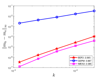
(a) Temporal accuracy in 1D

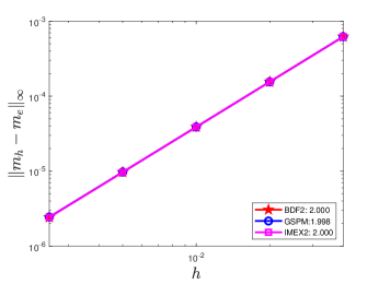
(b) Spatial accuracy in 1D

Figure 1: Accuracy test in 1D for BDF2, GSPM, and IMEX2 when $\alpha=1D-3$. (a) Temporal accuracy when $h=5D-4$; (b) Spatial accuracy when $k=1D-6$.

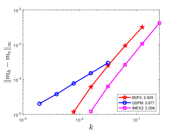
(a) Temporal accuracy in 3D

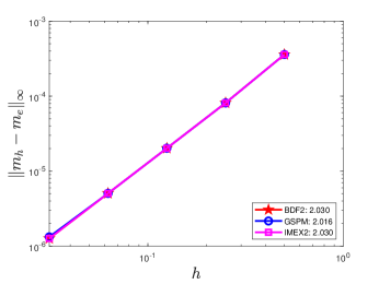
(b) Spatial accuracy in 3D

Figure 2: Accuracy test in 3D for BDF2, GSPM, and IMEX2 when $\alpha=1D-3$. (a) Temporal accuracy when $h_{x}=h_{y}=h_{z}=1/16$; (b) Spatial accuracy when $k=1D-4$.

3.4 Efficiency comparison

To compare the efficiency, we plot the CPU time (in seconds) of BDF2, GSPM and IMEX2 in terms of the error $\|\mbox{\boldmath$m$}_{h}-\mbox{\boldmath$m$}_{e}\|_{\infty}$ in fig. 3a for the 1D case and in fig. 3b for the 3D case.

In 1D, for the same tolerance, costs of BDF2, GSPM, and IMEX2 in fig. 3a satisfy: BDF2$<$IMEX2$<$GSPM. In 3D, for the same tolerance, costs of BDF2, GSPM, and IMEX2 in fig. 3b satisfy: BDF2$\approx$IMEX2$<$GSPM. For both cases, BDF2 is slightly better than IMEX2 since two linear systems of equations need to be solved in IMEX2 while only one linear system needs to solved in BDF2. Both BDF2 and IMEX2 are better than GSPM.

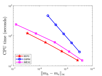
(a) 1D

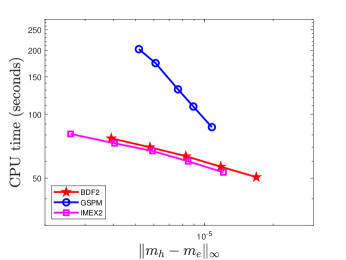
(b) 3D

Figure 3: Efficiency test for BDF2, GSPM, and IMEX2 when $\alpha=1D-3$ and the spatial gridsize is fixed. (a) BDF2$<$IMEX2$<$GSPM when $h=5D-4$ in 1D; (b) BDF2$\approx$ IMEX2$<$GSPM when $h_{x}=h_{y}=h_{z}=1/16$ in 3D.

Remark 6.

When the spatial mesh is very fine, we observe that to achieve the same tolerance, costs of BDF2, GSPM, and IMEX2 satisfy: GSPM$<$BDF2$<$IMEX2. The reason is that fast solvers can solve symmetric linear systems with constant coefficients in GSPM, while nonsymmetric linear systems with variable coefficients are involved in both BDF2 and IMEX2. It becomes increasingly difficult to solve such systems using the Generalized Minimum Residual Method (GMRES), for example. This issue will be further explored in a subsequent work.

4 Benchmark problem from NIST

To examine our methods in the realistic case, we simulate the first standard problem established by the micromagnetic modelling activity group at National Institute of Standards and Technology (NIST) [40]. This problem asks for simulating the hysteresis loop of a $L_{x}\times L_{y}\times L_{z}=1\times 2\times 0.02\;\mathrm{\mu m^{3}}$ thin-film element with material parameters that are not too different from Permalloy. The hysteresis loop is obtained in the following way: A positive external field of strength $H_{0}=\mu_{0}H_{e}$, in the unit of $mT$ is applied. The magnetization is able to reach a steady state. Once this steady state is approached, the applied external field is reduced by a certain amount, and the material sample is again allowed to reach a steady state. The process continues until the hysteresis system attains a negative field of strength $H_{0}$. The process then is repeated, increasing the field in small steps until it reaches the initial applied external field. As a consequence, we are able to plot the average magnetization at the steady state as a function of the external filed strength during the hysteresis loop. For BDF2, the unsymmetric linear systems of equations are solved by GMRES from library called high performance preconditioners [41] which was developed by Center for Applied Scientific Computing, Lawrence Livermore National Laboratory.

4.1 Magnetization profile

For comparison, we use the same setup of the available code mo96a of the first standard problem from NIST. Its setup is $100\times 50\times 1$ grid points and the canting angle $+1\degree$ of applied field from nominal axis. The calculation of the demagnetization field is done by FFT. The initial state is uniform. In the loop, $133$ successive steps between $+50\;\mathrm{mT}$ and $-50\;\mathrm{mT}$ are adopted for both x-loop and y-loop.

Due to the presence of meta-stable symmetric states, the applied fields should be rotated one degree counterclockwise off the nominal axis. The damping coefficient $\alpha=0.1$, the temporal stepsize $k=1\;\mathrm{ps}$ and the cell size is $20\times 20\times 20\;\mathrm{nm^{3}}$. A stopping criterion is used to determine that a steady state is reached when the relative change in the total energy is less than $10^{-7}$. For mo96a, LABEL:NIST_long_magnetization and LABEL:NIST_short_magnetization plot the average remanent magnetization on the bottom surface of the sample in the xy- plane when $H_{0}=0$ when the applied fields are approximately parallel (canting angle $+1\degree$) to the y- (long) axis and the x- (short) axis, respectively. For BDF2, the corresponding results are shown in LABEL:BDF2_long_magnetization and LABEL:BDF2_short_magnetization, respectively. The in-plane magnetization components are represented by arrows in LABEL:NIST_BDF2_magnetization.

Furthermore, magnetization components are visualized by the grayscale value in fig. 5. For mo96a, fig. 5a - fig. 5d plot the x- component and the y- component when the applied field is along the y- axis, the x- component and the y- component when the applied field is along the x- axis, respectively. Results of BDF2 are shown in Figures 5e, 5f, 5g and 5h.

From LABEL:NIST_BDF2_magnetization and fig. 5, we observe that results of BDF2 are in qualitative agreements with those of mo96a.

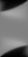
(a) $m_{x}\;(H_{0}//\textit{y-axis})$

(b) $m_{y}\;(H_{0}//\textit{y-axis})$

(c) $m_{x}\;(H_{0}//\textit{x-axis})$

(d) $m_{y}\;(H_{0}//\textit{x-axis})$

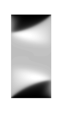
(e) $m_{x}\;(H_{0}//\textit{y-axis})$

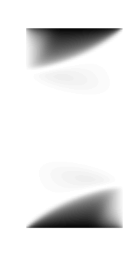
(f) $m_{y}\;(H_{0}//\textit{y-axis})$

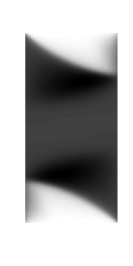
(g) $m_{x}\;(H_{0}//\textit{x-axis})$

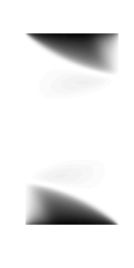
(h) $m_{y}\;(H_{0}//\textit{x-axis})$

Figure 5: Remanent magnetization when $\alpha=0.1$ for the bottom surface in the $xy$ plane. The applied field is approximately parallel (canting angle $+1\degree$) to the y- (long) axis (left two columns) and the x- (short) axis (right two columns). Top row: mo96a; Bottom row: BDF2. The x- and y- magnetization components are visualized by the gray value.

4.2 Hysteresis loop

Hysteresis loops generated by the code mo96a are shown in fig. 6a when the applied field is approximately parallel to the long axis and in fig. 6b when the applied field is approximately parallel to the short axis, respectively. The average remanent magnetization in reduced units is $(-0.15,0.87,0.00)$ for the y-loop and $(0.15,0.87,0.00)$ for the x-loop. The coercive fields are $4.9\;\mathrm{mT}$ in fig. 6a and $2.5\;\mathrm{mT}$ in fig. 6b.

For BDF2, hysteresis loops are presented in fig. 6c when the applied field is approximately parallel to the long axis and in fig. 6d when the applied field is approximately parallel to the short axis, respectively. The average remanent magnetization in reduced units is $(-1.613\times 10^{-1},8.606\times 10^{-1},-9.940\times 10^{-5})$ for the y-loop and $(1.681\times 10^{-1},8.571\times 10^{-1},-2.281\times 10^{-3})$ for the x-loop. The coercive fields are $5.213\,(\pm 0.4)\;\mathrm{mT}$ in fig. 6c and $2.552\,(\pm 0.4)\;\mathrm{mT}$ in fig. 6d.

Based on these results, we conclude that results of BDF2 agree well with those of NIST, both qualitatively and quantitatively.

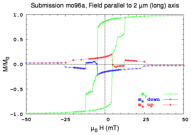
(a) $H_{0}//\textit{y-axis}$

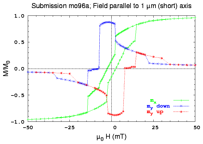
(b) $H_{0}//\textit{x-axis}$

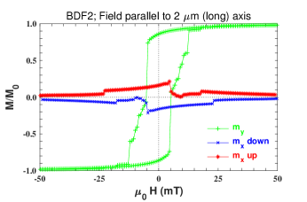
(c) $H_{0}//\textit{y-axis}$

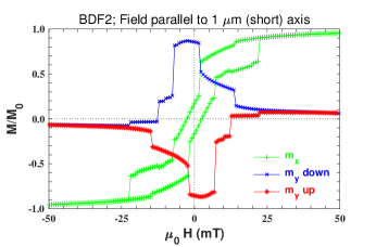
(d) $H_{0}//\textit{x-axis}$

Figure 6: Hysteresis loop when $\alpha=0.1$ and the cell size is $20\;\textrm{nm}\times 20\;\textrm{nm}\times 20\;\textrm{nm}$. The applied field is approximately parallel (canting angle $+1\degree$) to the y- (long) axis (left column) and the x- (short) axis (right column). Top row: mo96a; Bottom row: BDF2.

5 Conclusions

In this paper, we proposed two second-order semi-implicit projection methods to solve the Landau-Lifshitz-Gilbert equation, which possess unconditionally unique solvability at each time step. Examples in both 1D and 3D are used to verify the accuracy and the efficiency of both schemes. Additionally, the first benchmark problem from NIST is used to check the applicability of our methods in the realistic situation using the full Landau-Lifshitiz-Gilbert equation. Results show that our schemes can produce the correct hysteresis loop with quantities of interest agreeing with other methods in a quantitative manner.

One issue associated to the proposed methods is that nonsymmetric linear systems with variable coefficients are involved at each time step. It becomes increasingly difficult to solve such systems using the Generalized Minimum Residual Method. However, such linear systems have some unique features, as a consequence of the unique structure at the continuous level. This shall be used to develop more efficient linear solvers. Meanwhile, the technique presented here may be applicable to the model for current-driven domain wall dynamics [42] and the Schrödinger-Landau-Lifshitz system [43], which shall be explored later.

References

- Žutić et al. [2004] I. Žutić, J. Fabian, S. Das Sarma, Spintronics: Fundamentals and applications, Rev. Mod. Phys. 76 (2004) 323–410.
- Landau and Lifshitz [1935] L. Landau, E. Lifshitz, On the theory of the dispersion of magnetic permeability in ferromagnetic bodies, Phys. Z. Sowjet. 8 (1935) 153–169.
- Gilbert [1955] T. Gilbert, Phys. Rev. 100 (1955) 1243. [Abstract only; full report, Armor Research Foundation Project No. A059, Supplementary Report, May 1, 1956 (unpublished)].
- Shi et al. [1999] J. Shi, S. Tehrani, M. R. Scheinfein, Magnetization vortices and anomalous switching in patterned NiFeCo submicron arrays, Appl. Phys. Lett. 74 (1999) 2525–2527.
- Shi et al. [2000] J. Shi, T. Zhu, S. Tehrani, Y. Zheng, J.-G. Zhu, Geometry dependence of magnetization vortices in patterned submicron NiFe elements, Appl. Phys. Lett. 76 (2000) 2588–2590.
- Kruzík and Prohl [2006] M. Kruzík, A. Prohl, Recent developments in the modeling, analysis, and numerics of ferromagnetism, SIAM Rev. 48 (2006) 439–483.
- Cimrák [2008] I. Cimrák, A survey on the numerics and computations for the Landau-Lifshitz equation of micromagnetism, Arch. Comput. Method Eng. 15 (2008) 277–309.
- Abert et al. [2014] C. Abert, G. Hrkac, M. Page, D. Praetorius, M. Ruggeri, D. Suess, Spin-polarized transport in ferromagnetic multilayers: An unconditionally convergent FEM integrator, Comput. Math. Appl. 68 (2014) 639–654.
- Bruckner et al. [2014] F. Bruckner, D. Suess, M. Feischl, T. Führer, P. Goldenits, M. Page, D. Praetorius, M. Ruggeri, Multiscale modeling in micromagnetics: Existence of solutions and numerical integration, Math. Models Methods Appl. Sci. 24 (2014) 2627–2662.
- Baňas et al. [2014] L. Baňas, M. Page, D. Praetorius, J. Rochat, A decoupled and unconditionally convergent linear FEM integrator for the Landau–Lifshitz–Gilbert equation with magnetostriction, IMA J. Numer. Anal. 34 (2014) 1361–1385.
- Aurada et al. [2015] M. Aurada, J. Melenk, D. Praetorius, FEM–BEM coupling for the large-body limit in micromagnetics, J. Comput. Appl. Math. 281 (2015) 10–31.
- Le et al. [2015] K.-N. Le, M. Page, D. Praetorius, T. Tran, On a decoupled linear FEM integrator for eddy-current-LLG, Appl. Anal. 94 (2015) 1051–1067.
- Baňas et al. [2015] L. Baňas, M. Page, D. Praetorius, A convergent linear finite element scheme for the Maxwell-Landau-Lifshitz-Gilbert equation, Electron. Trans. Numer. Anal. 44 (2015) 250–270.
- Praetorius et al. [2018] D. Praetorius, M. Ruggeri, B. Stiftner, Convergence of an implicit–explicit midpoint scheme for computational micromagnetics, Comput. Math. Appl. 75 (2018) 1719–1738.
- Alouges and Jaisson [2006] F. Alouges, P. Jaisson, Convergence of a finite element discretization for the Landau-Lifshitz equations in micromagnetism, Math. Models Methods Appl. Sci. 16 (2006) 299–316.
- Alouges [2008] F. Alouges, A new finite element scheme for Landau-Lifchitz equations, Discrete Contin. Dyn. Syst. Ser. S 1 (2008) 187–196.
- Alouges et al. [2014a] F. Alouges, E. Kritsikis, J. Steiner, J.-C. Toussaint, A convergent and precise finite element scheme for Landau–Lifschitz–Gilbert equation, Numer. Math. 128 (2014a) 407–430.
- Alouges et al. [2014b] F. Alouges, A. de Bouard, A. Hocquet, A semi-discrete scheme for the stochastic Landau–Lifshitz equation, Stoch. Partial Differ. Equ. Anal. Comput. 2 (2014b) 281–315.
- E and Wang [2000] W. E, X. Wang, Numerical methods for the Landau-Lifshitz equation, SIAM J. Numer. Anal. 38 (2000) 1647–1665.
- Fuwa et al. [2012] A. Fuwa, T. Ishiwata, M. Tsutsumi, Finite difference scheme for the Landau-Lifshitz equation, Japan J. Indust. Appl. Math. 29 (2012) 83–110.
- Jeong and Kim [2010] D. Jeong, J. Kim, A Crank–Nicolson scheme for the Landau–Lifshitz equation without damping, J. Comput. Appl. Math. 234 (2010) 613–623.
- Kim and Lipnikov [2017] E. Kim, K. Lipnikov, The mimetic finite difference method for the Landau–Lifshitz equation, J. Comput. Phys. 328 (2017) 109–130.
- Romeo et al. [2008] A. Romeo, G. Finocchio, M. Carpentieri, L. Torres, G. Consolo, B. Azzerboni, A numerical solution of the magnetization reversal modeling in a permalloy thin film using fifth order Runge–Kutta method with adaptive step size control, Phys. B: Condens. Matter 403 (2008) 464 – 468.
- Jiang et al. [2001] J. S. Jiang, H. G. Kaper, G. K. Leaf, Hysteresis in layered spring magnets, Discrete Continuous Dyn. Syst. Ser. B. 1 (2001) 219–232.
- Prohl [2001] A. Prohl, Computational micromagnetism, volume 1, Springer, 2001.
- Bartels and Prohl [2006] S. Bartels, A. Prohl, Convergence of an implicit finite element method for the Landau-Lifshitz-Gilbert equation, SIAM J. Numer. Anal. 44 (2006) 1405–1419.
- Wang et al. [2001] X. Wang, C. J. García-Cervera, W. E, A Gauss-Seidel projection method for micromagnetics simulations, J. Comput. Phys. 171 (2001) 357–372.
- García-Cervera and E [2003] C. J. García-Cervera, W. E, Improved Gauss-Seidel projection method for micromagnetics simulations, IEEE Trans. Magn. 39 (2003) 1766–1770.
- Lewis and Nigam [2003] D. Lewis, N. Nigam, Geometric integration on spheres and some interesting applications, J. Comput. Appl. Math. 151 (2003) 141–170.
- Cimrák [2005] I. Cimrák, Error estimates for a semi-implicit numerical scheme solving the Landau-Lifshitz equation with an exchange field, IMA J. Numer. Anal. 25 (2005) 611–634.
- Gao [2014] H. Gao, Optimal error estimates of a linearized Backward Euler FEM for the Landau-Lifshitz equation, SIAM J. Numer. Anal. 52 (2014) 2574–2593.
- Boscarino et al. [2016] S. Boscarino, F. Filbet, G. Russo, High order semi-implicit schemes for time dependent partial differential equations, J. Sci. Comput. 68 (2016) 975–1001.
- Jeong and Kim [2014] D. Jeong, J. Kim, An accurate and robust numerical method for micromagnetics simulations, Curr. Appl. Phys. 14 (2014) 476–483.
- Cimrák and Slodička [2004] I. Cimrák, M. Slodička, An iterative approximation scheme for the Landau-Lifshitz-Gilbert equation, J. Comput. Appl. Math. 169 (2004) 17–32.
- Chen et al. [2019] J. Chen, C. Wang, C. Xie, Convergence analysis of a second-order semi-implicit projection method for Landau-Lifshitz equation, 2019. ArXiv preprint arXiv: 1902.09740.
- Jr. [1963] W. F. B. Jr., Micromagnetics, Interscience Tracts on Physics and Astronomy. Interscience Publishers (John Wiley and Sons), New York-London, 1963.
- Browder [1963] F. E. Browder, Nonlinear elliptic boundary value problems, Bull. Amer. Math. Soc. 69 (1963) 862–874.
- Minty [1963] G. J. Minty, On a monotonicity method for the solution of non-linear equations in Banach spaces, Proc. Nat. Acad. Sci. 50 (1963) 1038–1041.
- Prasolov [1994] V. V. Prasolov, Problems and theorems in linear algebra, volume 134, Amer. Math. Soc., 1994.
- Micromagnetic Modeling Activity Group [2000] Micromagnetic Modeling Activity Group, National Institute of Standards and Technology, 2000. URL: https://www.ctcms.nist.gov/~rdm/mumag.org.html.
- Center for Applied Scientific Computing, Lawrence Livermore National Laboratory [1952] Center for Applied Scientific Computing, Lawrence Livermore National Laboratory, HYPRE: Scalable Linear Solvers and Multigrid Methods, 1952. URL: https://computation.llnl.gov/projects/hypre-scalable-linear-solvers-multigrid-methods.
- Chen et al. [2015] J. Chen, C. J. García-Cervera, X. Yang, A mean-field model of spin dynamics in multilayered ferromagnetic media, Multiscale Model. Simul. 13 (2015) 551–570.
- Chen et al. [2016] J. Chen, J.-G. Liu, Z. Zhou, On a Schrödinger–Landau–Lifshitz system: Variational structure and numerical methods, Multiscale Model. Simul. 14 (2016) 1463–1487.