Gradient-Adaptive Spline-Interpolated LUT Methods for Low-Complexity Digital Predistortion

Abstract

In this paper, new digital predistortion (DPD) solutions for power amplifier (PA) linearization are proposed, with particular emphasis on reduced processing complexity in future 5G and beyond wideband radio systems. The first proposed method, referred to as the spline-based Hammerstein (SPH) approach, builds on complex spline-interpolated lookup table (LUT) followed by a linear finite impulse response (FIR) filter. The second proposed method, the spline-based memory polynomial (SMP) approach, contains multiple parallel complex spline-interpolated LUTs together with an input delay line such that more versatile memory modeling can be achieved. For both structures, gradient-based learning algorithms are derived to efficiently estimate the LUT control points and other related DPD parameters. Large set of experimental results are provided, with specific focus on 5G New Radio (NR) systems, showing successful linearization of multiple sub-6 GHz PA samples as well as a 28 GHz active antenna array, incorporating channel bandwidths up to 200 MHz. Explicit performance-complexity comparisons are also reported between the SPH and SMP DPD systems and the widely-applied ordinary memory-polynomial (MP) DPD solution. The results show that the linearization capabilities of the proposed methods are very close to that of the ordinary MP DPD, particularly with the proposed SMP approach, while having substantially lower processing complexity.

I Introduction

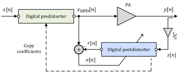
(a)

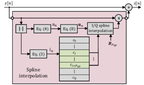
(b)

Figure 1:  Illustration of a) the considered DPD system building on indirect learning architecture (ILA), and b) the injection-based complex spline-interpolated LUT scheme utilized inside the proposed digital predistorter and digital postdistorter entities.

Modern radio communication systems, such as the 4G LTE/LTE-Advanced and the emerging 5G New Radio (NR) mobile networks, build on multicarrier modulation, most notably orthogonal frequency division multiplexing (OFDM)[1]. OFDM waveforms are known to contain high peak-to-average power-ratio (PAPR)[2, 3], which complicates utilizing highly nonlinear power amplifiers (PAs) in transmitters operating close to saturation [2, 4, 5]. Digital pre-distortion (DPD) is, generally, a well-established approach to control the unwanted emissions and nonlinear distortion stemming from nonlinear PAs, see, e.g.,[2, 6, 7, 4, 8, 9] and references therein. Especially when combined with appropriate PAPR reduction methods [10], DPD based systems can largely improve the transmitter power efficiency while keeping the unwanted emissions within specified limits.

Some of the most common approaches in PA direct modeling as well as DPD processing are the memory polynomial (MP)[9, 2, 11] and the generalized memory polynomial (GMP)[12, 13, 2, 11], both of which can be interpreted to be special cases of the Volterra series[2, 14, 15, 16]. Such approaches allow for efficient direct and inverse modeling of nonlinear systems with memory, while also supporting straight-forward parameter estimation, through, e.g., linear least-squares (LS), as they are known to be linear-in-parameters models[11]. However, the processing complexity per linearized sample is also relatively high, particularly with GMP and other more complete Volterra series type of approaches, though also some works exist where complexity reduction is pursued [15, 17, 18, 19, 20, 21]. Specifically, the works in [18, 19, 22] present predistorter and PA modeling methods that build on spline-based basis functions – an approach that is technically considered also in this article, in the form of spline-interpolated lookup tables (LUTs).

In this paper, we develop and describe two new DPD solutions whose linearization capabilities are similar to those of the well-established polynomial-based solutions, while at the same time offering a substantially reduced DPD main path processing and parameter learning complexities. The development of such reduced-complexity DPD solutions is mainly motivated by the following four facts or tendencies. First, the channel bandwidths in NR are substantially larger than those in LTE-based systems. Specifically, up to 100 MHz and 400 MHz continuous channel bandwidths are already specified in NR Release-15 at frequency range 1 (FR-1; below 6 GHz bands) and FR-2 (24-40 GHz bands), respectively, [23], which imply increased DPD processing rates. Second, the actual unwanted emission requirements, particularly in the form of total radiated power (TRP) based adjacent channel leakage ratio (ACLR), are largely relaxed in NR FR-2 systems, being only in the order of 26-28 dB [23], increasing the feasibility of simplified DPD solutions. Third, the medium range and local area base-stations adopt substantially reduced transmit powers [23], compared to classical macro base-stations, hence the available power budget of the DPD solutions is also reduced. Finally, as observed recently in [5], even continuous learning may be needed at FR-2 and other mmWave active array systems, hence developing methods which reduce the parameter learning complexity becomes important.

The first new DPD method proposed in this paper, referred to as the spline-based Hammerstein (SPH) approach, builds on complex spline-interpolated LUT followed by a linear finite impulse response (FIR) filter. The interpolation allows to use a small amount of points in the LUT, while the linear filter facilitates basic memory modeling. Gradient-based learning algorithms are also derived, to efficiently estimate the LUT control points as well as the linear filter parameters in a decoupled manner. The second proposed DPD method, referred to as the spline-based memory polynomial (SMP), consists of multiple parallel spline-interpolated LUTs and an input delay line such that more versatile memory modeling can be achieved when summing together the outputs of the parallel LUTs. Through spline interpolation, the size of all parallel LUTs can be kept small, while gradient-adaptive learning rule is again derived to estimate the control points of the involved parallel LUTs. For both proposed models – the SPH DPD and the SMP DPD – comprehensive computational complexity analyses are provided, while also comparing to ordinary gradient-adaptive canonical MP DPD system. Then, extensive RF measurement results are provided, covering several different FR-1 PA samples, channel bandwidth cases as well as base-station classes. Additionally, a state-of-the-art 28 GHz active antenna array, specifically Anokiwave AWMF-0129, is successfully linearized with 100 MHz and 200 MHz 5G NR channel bandwidths.

In general, it is noted that LUT-based PA linearization is, as such, a well-known approach, see, e.g., [8, 24, 25, 26, 27] and the references therein. However, the PA memory aspects are not considered in [24], while fairly sizeable LUTs without interpolation are considered in [8, 26]. Additionally, a linearly-interpolated LUT-type implementation of a memory polynomial is described in [25] while the learning is based on classical LS model fitting. Furthermore, in [27], a DPD structure that includes two parallel Hammerstein systems compensating for the PA AM-AM and AM-PM responses, with Catmull-Rom spline interpolation, is presented. The model identification is based on a separable LS technique, specifically using a Levenberg-Marquardt algorithm to identify the DPD coefficients. The main path and training complexities are thus high when compared to the methods presented in this article. It is finally also noted that multi-dimensional LUT based solutions exist [28, 29]. However, the LUT size in the nested LUT scheme in [28] grows exponentially with the memory depth, thus requiring unfeasible total LUT size when the linearized system exhibits substantial memory. The 2-dimensional LUT technique in [29] is, in turn, limited in its memory modeling capability, since it uses a weighted average of past amplitude samples to index the second LUT dimension.

In the DPD system context of Fig. 1, the novelty and contributions of this article can be summarized as follows:

• New linear-in-parameters formulation for utilizing spline-interpolated I/Q LUTs in DPD systems, incorporating also the so-called injection-based DPD structure, is provided;

• New Hammerstein DPD solution utilizing the spline-interpolated I/Q LUT and decoupled gradient-based learning is proposed and derived;

• New memory polynomial DPD solution utilizing multiple parallel spline-interpolated I/Q LUTs and gradient-based learning is proposed and derived;

• Comprehensive computational complexity analysis of the methods is provided;

• Extensive performance-complexity assessments using versatile RF measurement examples at sub-6 GHz and 28 GHz bands are provided;

Compared to the existing literature, the new DPD formulation with spline-interpolated I/Q LUTs allows, in general, for (i) using any typical linear estimator (gradient or least-squares) to learn or update the LUT entries and (ii) reducing the main path processing complexity clearly when compared to ordinary canonical MP DPD. Specifically, the main path complexity and particularly the learning complexity are both reduced when compared to gradient-based canonical MP, owing to the use of the derived gradient-based learning in combination with the interpolated LUTs, since no basis function orthogonalization [7] nor self-orthogonalized learning procedure [30, 25] is needed with the proposed methods. Thus, even continuous DPD adapting/tracking is potentially viable.

The rest of the paper is organized as follows. Section II describes the I/Q spline interpolation scheme used throughout this paper, and presents the proposed SPH and SMP predistorter models. Section III derives and presents then the gradient-descent parameter learning algorithms for both DPD models. A complexity analysis and comparison of the proposed DPD solutions is provided in Section IV. Section V describes the RF measurement setups, and presents the corresponding measurement results and their analyses. Finally, conclusions are drawn in Section VI.

Throughout the rest of this article, matrices are denoted by capital boldface letters, e.g., $\mathbf{A}\in\mathbb{C}^{(M\times N)}$, while vectors are denoted by lowercase boldface letters, e.g. , $\mathbf{v}\in\mathbb{C}^{M\times 1}=[v_{1}\ v_{2}\ \cdots\ v_{M}]^{T}$. Ordinary transpose and hermitian operators are represented as $(\cdot)^{T}$ and $(\cdot)^{H}$, respectively. Additionally, the absolute value, floor, and ceil operators are represented as $\absolutevalue{\,\cdot\,}$, $\left\lfloor\cdot\right\rfloor$, and $\left\lceil\cdot\right\rceil$, respectively.

II Proposed DPD Models

In this section, we introduce the proposed I/Q spline interpolation scheme, followed by the corresponding formulation of the SPH and SMP DPD models. For notational convenience, we formulate the mathematical presentation in the context of the indirect learning architecture (ILA) for postdistorter processing, with $z[n]$ and $r[n]$ denoting the postdistorter input and output, respectively. In the actual predistortion stage – as illustrated also in Fig. 1 – the input and output signals are $x[n]$ and $x_{\mathrm{DPD}}[n]$, respectively.

II-A Background and Basics

Building on piece-wise polynomials, spline based modeling and interpolation seeks to determine a smooth curve that approximates or conforms to a set of points, commonly known as control points [31]. Consequently, the input signal range is divided into several pieces, and the polynomials model the nonlinear system behavior in the corresponding regions under continuity and smoothness constraints. With this approach, simple low-order functions can be adopted, per region, in contrast to methods where a single high-order function or polynomial seeks to model the whole input range.

Traditionally, spline modeling has been applied to real-valued signals and systems [31, 32, 33, 34]. However, in the context of radio communications, complex I/Q signals are utilized, and therefore the spline models need to be extended to the complex domain. Specifically, in this paper, we consider complex baseband models of RF nonlinearities, particularly those stemming from PA, for DPD purposes. To first shortly illustrate how splines can be applied to RF nonlinearity modelling at baseband, we start with the well-known memoryless polynomial, written for an arbitrary input signal $x_{\mathrm{in}}[n]$ as

$$x_{\mathrm{out}}[n]=\sum_{\begin{subarray}{c}p=0,\hskip 2.84526ptp\mathrm{\,odd}\end{subarray}}^{P}\alpha_{p}x_{\mathrm{in}}[n]\absolutevalue{x_{\mathrm{in}}[n]}^{p-1},$$ (1)

where $\alpha_{p}\in\mathbb{C}$ are the corresponding polynomial coefficients [9, 12]. Setting $\alpha_{1}=1$, without loss of generality, this can be re-written as

$$x_{\mathrm{out}}[n] =x_{\mathrm{in}}[n](1+\alpha_{3}\absolutevalue{x_{\mathrm{in}}[n]}^{2}+\cdots+\alpha_{P}\absolutevalue{x_{\mathrm{in}}[n]}^{P-1})$$

$$=x_{\mathrm{in}}[n](1+F(\absolutevalue{x_{\mathrm{in}}[n]})),$$ (2)

where the function $F(\cdot)=F_{\mathrm{I}}(\cdot)+jF_{\mathrm{Q}}(\cdot)$ is a real-to-complex mapping. Thus, the baseband equivalent nonlinearity model consists of two real-valued functions $F_{\mathrm{I}}(\cdot)$ and $F_{\mathrm{Q}}(\cdot)$, both dependent only on the absolute value of the input signal.

II-B Proposed I/Q Spline Interpolation Scheme

In general, the above model structure shown in (2) can be used for both PA direct modeling as well as PA inverse modeling, i.e., DPD. In the context of DPD – which is the focus of this article – the nonlinear functions can be implemented efficiently with, for example, LUTs.

To this end, in the linearization context of Fig. 1, we formulate in this article spline-interpolated LUTs, i.e., small LUTs with spline interpolation to obtain the intermediate values. By adopting the notations in Fig. 1, such spline-based modeling of the nonlinear functions $F_{\mathrm{I}}(\cdot)$ and $F_{\mathrm{Q}}(\cdot)$ is illustrated at conceptual level in Fig. 2, where the input is a unipolar signal $\absolutevalue{z[n]}$ with a maximum amplitude of $A_{\max}$. We adopt uniform equi-spaced splines with knot spacing (region width) of $\Delta_{z}>0$, thus resulting in a total of $K=A_{\max}/\Delta_{z}$ regions. These regions are built, and accessed at time instant $n$, through the span index $i_{n}$ and abscissa value $u_{n}$, defined as

$$i_{n} =\left\lfloor\frac{\absolutevalue{z[n]}}{\Delta_{z}}\right\rfloor+1,$$ (3)

$$u_{n} =\frac{\absolutevalue{z[n]}}{\Delta_{z}}-(i_{n}-1).$$ (4)

Here, $i_{n}$ denotes the index of the selected region at time instant $n$, and $u_{n}$, $0\!\leq\!u_{n}\!<\!\Delta_{z}$, represents the normalized value of the corresponding input envelope within the current region $i_{n}$.

Figure 2:  Conceptual illustration of the nonlinear model regions of $F_{\mathrm{I}}(\absolutevalue{z[n]})$ and $F_{\mathrm{Q}}(\absolutevalue{z[n]})$ with respect the input magnitude $\absolutevalue{z[n]}$ assuming $K=5$ regions. Also an example of the input envelope value is shown, in this particular case within region $i_{n}=4$, where $u_{n}\in[0,\Delta_{z})$ denotes the normalized input envelope within a region.

In general, adopting uniform splines allows the spline-interpolated output signal to take a very simple form, discussed also in [27] in the context of real-valued systems. The outputs of the I and Q splines can now be written as

$$F_{\mathrm{I}}(\absolutevalue{z[n]}) =\mathbf{g}_{n}^{T}\mathbf{c}^{\mathrm{re}},$$ (5)

$$F_{\mathrm{Q}}(\absolutevalue{z[n]}) =\mathbf{g}_{n}^{T}\mathbf{c}^{\mathrm{im}},$$ (6)

where $\mathbf{c}^{\mathrm{re}}$ and $\mathbf{c}^{\mathrm{im}}$ contain the $Q$ control points of each spline. The vector $\mathbf{g}_{n}$ $\in\mathbb{R}^{Q\times 1}$, in turn, is defined as

$$\mathbf{g}_{n}=\begin{bmatrix}0&\cdots&0&\mathbf{u}_{n}^{T}\,\mathbf{B}_{P_{\mathrm{SP}}}&0&\cdots&0\end{bmatrix}^{T},$$ (7)

where

$$\mathbf{u}_{n}=\begin{bmatrix}u_{n}^{P_{\mathrm{SP}}}&u_{n}^{P_{\mathrm{SP}}-1}&\cdots&1\end{bmatrix}^{T}\in\mathbb{R}^{(P_{\mathrm{SP}}+1)\times 1},$$ (8)

and $\mathbf{B}_{P_{\mathrm{SP}}}\in\mathbb{R}^{(P_{\mathrm{SP}}+1)\times(P_{\mathrm{SP}}+1)}$ is the spline basis matrix of order $P_{\mathrm{SP}}$. In (7), the term $\mathbf{u}_{n}^{T}\mathbf{B}_{P_{\mathrm{SP}}}$ of size $1\times(P_{\mathrm{SP}}+1)$ is located such that the starting index is $i_{n}$. Thus, at a given time instant $n$, only the control points $c_{i_{n}},c_{i_{n}+1},\ldots,c_{i_{n}+P_{\mathrm{SP}}}$ contribute to the output. It is noted that for simplicity, we assume in this work that the spline order $P_{\mathrm{SP}}$ does not depend on the region.

Using (5) and (6), while following the model structure in (2), the complex-valued output of the instantaneous nonlinear system, $s[n]$, can be constructed as

$$s[n] =z[n]+z[n]\mathbf{g}_{n}^{T}(\mathbf{c}^{\mathrm{re}}+j\mathbf{c}^{\mathrm{im}})$$

$$=z[n]+z[n]\mathbf{g}_{n}^{T}\mathbf{c},$$ (9)

where $\mathbf{c}\in\mathbb{C}^{Q\times 1}=\begin{bmatrix}c_{0}&c_{1}&\cdots&c_{Q-1}\end{bmatrix}^{T}$ is the overall complex-valued LUT containing the control points for the I and Q components. The interpolation scheme is further detailed in Fig. 1(b). We also note that the total number of control points with $K$ regions and spline interpolation order $P_{\mathrm{SP}}$ is $Q=K+P_{\mathrm{SP}}$.

Importantly, the spline output $\mathbf{g}_{n}^{T}\mathbf{c}$ in (9) is defined as a deviation from unit gain. We refer to such structure as an injection-based scheme. Specifically, with this formulation, if $\mathbf{c}$ is initialized as an all-zero vector, the nonlinear system output will be the original input signal, i.e. $s[n]=z[n]$. By following this formulation, e.g., the gain ambiguities between the nonlinear spline and a cascaded FIR filter can be effectively removed – an issue that is relevant in the following Hammerstein DPD system – as the linear filter alone will handle the gain in the system. Additionally, the number of required bits in $\mathbf{c}$ in a fixed-point implementation is generally reduced, as this formulation reduces its dynamic range.

II-C Spline-Interpolated Hammerstein DPD

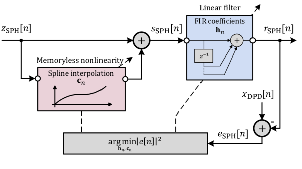
(a)

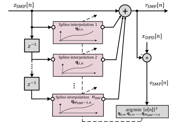
(b)

Figure 3:  Illustration of the postdistorter structures of a) the proposed SPH DPD system, and b) the proposed SMP DPD model. The Spline interpolation block(s) in both models comprises the scheme shown in Fig. 1(b).

This subsection introduces the proposed SPH scheme which builds on a Hammerstein structure where the involved nonlinearity is modelled with a complex spline-interpolated LUT. Following the proposed interpolation scheme presented above, in (9), we thus express the output of the instantaneous nonlinear block in the Hammerstein structure as

$${\color[rgb]{0,0,0}s_{\mathrm{SPH}}[n]=z_{\mathrm{SPH}}[n]+z_{\mathrm{SPH}}[n]\mathbf{g}_{n}^{T}\mathbf{c}.}$$ (10)

It is noted that the term $\mathbf{g}_{n}$ depends on the B-spline basis matrix $\mathbf{B}_{P_{\mathrm{SP}}}$. This matrix can be precomputed for the given type of splines and polynomial order, and can be therefore considered as static. As a concrete example, in this article we focus on 3^rd order ($P_{\mathrm{SP}}=3$, cubic interpolation) B-splines, although other spline orders are tested and demonstrated as well. In this case, the basis matrix can be expressed as [32]

$$\mathbf{B}_{3}=\frac{1}{6}\begin{bmatrix}\frac{-1}{\Delta_{z}^{3}}&\frac{3}{\Delta_{z}^{3}}&\frac{-3}{\Delta_{z}^{3}}&\frac{1}{\Delta_{z}^{3}}\\[5.0pt] \frac{3}{\Delta_{z}^{2}}&\frac{-6}{\Delta_{z}^{2}}&\frac{3}{\Delta_{z}^{2}}&0\\[5.0pt] \frac{-3}{\Delta_{z}}&0&\frac{3}{\Delta_{z}}&0\\[5.0pt] 1&4&1&0\end{bmatrix}.$$ (11)

Next, after having derived the expression for the memoryless nonlinear signal model, the memory effects are incorporated through the FIR filter stage that is common to all regions. Hence, the overall output signal $r_{\mathrm{SPH}}[n]$ can be directly expressed as

$$r_{\mathrm{SPH}}[n]=\mathbf{h}^{T}\mathbf{s}_{n},$$ (12)

where $\mathbf{h}\in\mathbb{C}^{M_{\mathrm{SPH}}\times 1}=\begin{bmatrix}h_{0}&h_{1}&\cdots&h_{M_{\mathrm{SPH}}-1}\end{bmatrix}^{T}$ contains the filter coefficients, with $M_{\mathrm{SPH}}$ denoting the number of taps in the model, while $\mathbf{s}_{n}\in\mathbb{C}^{M_{\mathrm{SPH}}\times 1}=\begin{bmatrix}s_{\mathrm{SPH}}[n]&s_{\mathrm{SPH}}[n-1]&\cdots&s_{\mathrm{SPH}}[n-M_{\mathrm{SPH}}+1]\end{bmatrix}^{T}$. The overall processing structure is illustrated in Fig. 3(a).

II-D Spline-Interpolated MP LUT DPD

This subsection formulates the proposed SMP DPD model. Inspired by [8], a memory polynomial type parallel branched structure is adopted to model the memory effects, while the actual parallel nonlinearities are each implemented through the complex spline-interpolated LUTs presented above. To this end, the proposed SMP processing can thus be expressed as

$$r_{\mathrm{SMP}}[n]=z_{\mathrm{SMP}}[n]+\sum_{m=0}^{M_{\mathrm{SMP}}-1}z_{\mathrm{SMP}}[n-m]\mathbf{g}_{n-m}^{T}\mathbf{q}_{m},$$ (13)

where $M_{\mathrm{SMP}}$ denotes the considered memory order while $\mathbf{q}_{m}$, $m=0,1,\ldots,M_{\mathrm{SMP}}-1$, are the $M_{\mathrm{SMP}}$ LUTs of the model, containing the control points for the spline interpolation in each parallel branch. The proposed SMP processing structure, adopting also the injection principle but in generalized form, is illustrated in Fig. 3(b).

In general, in terms of the modeling capabilities, the SMP is a richer model compared to SPH, while it also naturally entails higher complexity. These models will be assessed and compared to classical DPD solutions in terms of complexity and performance in Sections IV and V.

III Parameter Learning Rules

In this section, we derive efficient gradient-descent type learning rules for both proposed DPD approaches, to adaptively estimate and track the unknown parameters in each of the models. Notation-wise, to allow for sample-adaptive estimation, we denote the vectors to be estimated with a subindex $n$, i.e., $\mathbf{c}_{n}$ and $\mathbf{h}_{n}$ for SPH and $\mathbf{q}_{m,n}$, $m=0,1,\ldots,M_{\mathrm{SMP}}-1$, for SMP, to indicate their time-dependence.

III-A SPH Learning Rules

To calculate the learning rule in the SPH case, the instantaneous error signal between $x_{\mathrm{DPD}}[n]$ and $r_{\mathrm{SPH}}[n]$, in the context of the considered ILA-type architecture is first extracted as

$$e_{\mathrm{SPH}}[n]=x_{\mathrm{DPD}}[n]-r_{\mathrm{SPH}}[n]=x_{\mathrm{DPD}}[n]-\mathbf{h}_{n}^{T}\mathbf{s}_{n}.$$ (14)

Then, to facilitate the gradient-descent learning [35], the cost function is defined as the instantaneous squared error, expressed as

$$J(\mathbf{h}_{n},\mathbf{c}_{n})=\absolutevalue{e_{\mathrm{SPH}}[n]}^{2}.$$ (15)

The corresponding iterative learning rules are then obtained through the partial derivatives of $J(\mathbf{h}_{n},\mathbf{c}_{n})$ with respect both parameter vectors to adapt, expressed formally as

$$\mathbf{h}_{n+1} =\mathbf{h}_{n}-\mu_{\mathrm{h}}[n]\mathbf{\nabla}_{\mathbf{h}_{n}}J(\mathbf{h}_{n},\mathbf{c}_{n}),$$ (16)

$$\mathbf{c}_{n+1} =\mathbf{c}_{n}-\mu_{\mathrm{c}}[n]\mathbf{\nabla}_{\mathbf{c}_{n}}J(\mathbf{h}_{n},\mathbf{c}_{n}),$$ (17)

where $\mathbf{\nabla}_{\mathbf{x}}$ refers to the complex gradient operator [35, 36] of a real-valued function against complex-valued parameter vector $\mathbf{x}$. Additionally, $\mu_{\mathrm{h}}[n]$ and $\mu_{\mathrm{c}}[n]$ are the learning rates for $\mathbf{h}_{n}$ and $\mathbf{c}_{n}$, respectively, at time instant $n$. After relatively straight-forward derivations, the resulting concrete learning rules read

$$\mathbf{h}_{n+1} =\mathbf{h}_{n}+\mu_{\mathrm{h}}[n]e_{\mathrm{SPH}}[n]\mathbf{s}_{n}^{*},$$ (18)

$$\mathbf{c}_{n+1} =\mathbf{c}_{n}+\mu_{\mathrm{c}}[n]e_{\mathrm{SPH}}[n]\mathbf{\Sigma}_{n}^{T}\mathbf{Z}_{n}^{*}\mathbf{h}_{n}^{*},$$ (19)

where the diagonal matrix $\mathbf{Z}_{n}\in\mathbb{C}^{M_{\mathrm{SPH}}\times M_{\mathrm{SPH}}}=\operatorname{diag}\left\{z_{\mathrm{SPH}}[n],\;z_{\mathrm{SPH}}[n-1],\;\cdots,\;z_{\mathrm{SPH}}[n-M_{\mathrm{SPH}}+1]\right\}$, and $\mathbf{\Sigma}_{n}$ contains $M_{\mathrm{SPH}}$ previous instances of $\mathbf{g}_{n}$, defined as $\mathbf{\Sigma}_{n}\in\mathbb{R}^{M_{\mathrm{SPH}}\times Q}=\begin{bmatrix}\mathbf{g}_{n}&\mathbf{g}_{n-1}&\cdots&\mathbf{g}_{n-M_{\mathrm{SPH}}+1}\end{bmatrix}^{T}$. These learning rules in (18) and (19) are executed in parallel such that both parameter vectors are updated simultaneously. For readers’ convenience, an example illustration of the structure of the matrix $\mathbf{\Sigma}_{n}$ is given in (25), for $M_{\mathrm{SPH}}=4$, $Q=9$, and $P_{\mathrm{SP}}=3$, assuming representative example values of the index variable $i_{n}$.

$$\mathbf{\Sigma}_{n}=\begin{bmatrix}0\quad 0\quad\underbrace{[*\quad*\quad*\quad*]}_{\mathbf{u}_{n}^{T}\mathbf{B}_{P_{\mathrm{SP}}}}\quad 0\quad 0\quad 0\\ \underbrace{[*\quad*\quad*\quad*]}_{\mathbf{u}_{n-1}^{T}\mathbf{B}_{P_{\mathrm{SP}}}}\quad 0\quad 0\quad 0\quad 0\quad 0\\ 0\quad 0\quad 0\quad\underbrace{[*\quad*\quad*\quad*]}_{\mathbf{u}_{n-2}^{T}\mathbf{B}_{P_{\mathrm{SP}}}}\quad 0\quad 0\\ 0\quad 0\quad 0\quad 0\quad 0\quad\underbrace{[*\quad*\quad*\quad*]}_{\mathbf{u}_{n-3}^{T}\mathbf{B}_{P_{\mathrm{SP}}}}\\ \end{bmatrix},\begin{array}[]{l}i_{n}=3\\[17.0pt] i_{n-1}=1\\[17.0pt] i_{n-2}=4\\[17.0pt] i_{n-3}=6\\[3.0pt] {\color[rgb]{1,1,1}.}\end{array}$$ (25)

Note that the term $\mathbf{u}_{n}^{T}\mathbf{B}_{P_{\mathrm{SP}}}$ is located in $\mathbf{\Sigma}_{n}$ at each iteration $n$ according to the span index $i_{n}$, as shown in (7). It is noted that the derived learning rules in (18) and (19) are novel, as the overall Hammerstein system is known to be not linear in its parameters.

III-B SMP Learning Rules

We next derive gradient-based iterative learning rules for the SMP model. Different to SPH case, the SMP model does not contain cascaded filters while the learning entity considers the $M_{\mathrm{SMP}}$ parallel spline-interpolated LUTs, specifically their control points $\mathbf{q}_{m,n}$, $m=0,1,\ldots,M_{\mathrm{SMP}}-1$.

Following now a similar approach as earlier, the instantaneous error signal is first defined in the context of ILA-based learning as

$$e_{\mathrm{SMP}}[n] =\!x_{\mathrm{DPD}}[n]-r_{\mathrm{SMP}}[n]$$

$$=\!x_{\mathrm{DPD}}[n]-z_{\mathrm{SMP}}[n]\!-\!\!\!\sum_{m=0}^{M_{\mathrm{SMP}}-1}\!\!z_{\mathrm{SMP}}[n-m]\mathbf{g}_{n-m}^{T}\mathbf{q}_{m,n}.$$ (26)

For the gradient-descent learning, the cost function is defined as a function of the instantaneous error signal as

$$J(\mathbf{q}_{0,n},\mathbf{q}_{1,n},\cdots,\mathbf{q}_{M_{\mathrm{SMP}}-1,n})=\absolutevalue{e_{\mathrm{SMP}}[n]}^{2}.$$ (27)

Then, by adopting again the complex gradient operator [36], the learning rule for the $m$th LUT can be written as

$$\mathbf{q}_{m,n+1}=\mathbf{q}_{m,n}-\mu_{\mathrm{q}_{m}}\mathbf{\nabla}_{\mathbf{q}_{m,n}}J(\mathbf{q}_{0,n},\mathbf{q}_{1,n},\cdots,\mathbf{q}_{M_{\mathrm{SMP}}-1,n}),$$ (28)

while by following the complex differentiation steps, the final learning rule for the $m$th LUT reads

$$\mathbf{q}_{m,n+1}=\mathbf{q}_{m,n}+\mu_{\mathrm{q}_{m}}[n]\;e_{\mathrm{SMP}}[n]\;z_{\mathrm{SMP}}^{*}[n-m]\;\mathbf{g}_{n-m}.$$ (29)

These learning rules are adopted for all the involved $M_{\mathrm{SMP}}$ LUTs in parallel.

IV Computational Complexity Analysis

In this section, a computational complexity analysis and comparison between the proposed SPH, SMP and a widely-applied canonical MP DPD with self-orthogonalizing least-mean square (LMS) [35] parameter adaptation is presented. LMS type adaptation is deliberately assumed also for MP DPD, for the fairness of the comparison. The complexity analysis is carried out in terms of real multiplications per linearized data sample, as multiplications are commonly more resource-intensive operations than additions in digital signal processing (DSP) implementations [11].

The quantitative complexity assessment of the proposed gradient-adaptive SPH DPD and SMP DPD follows the exact processing steps described in Sections II and III. It is noted that the complexity expressions reported below basically represent an upper bound for the required arithmetical operations, as in real implementations some elementary or trivial operations such as multiplying by any integer power of $2$ or $1/2$ does not really reflect any actual complexity, while are included as normal operations in the expressions for simplicity. Additionally, it is noted that the modulus operator, needed in (3) and (4), is assumed to be calculated with the alpha max beta min algorithm [37]. Finally, in the complexity analysis, we consider uniform splines with $\Delta_{z}=\Delta_{x}=1$.

IV-A Complexity of Proposed SPH Method

With reference to Fig. 3(a) and the underlying processing elements, the generic complexity expressions can be stated in a straight-forward manner as follows:

• DPD main path, starting with the input signal $x[n]$. The complexity of the predistorter intermediate signal, $s_{\mathrm{DPD}}[n]$, includes the processing in (3), (4), and (10) but with $x[n]$ as the input. These together with the FIR filtering in (12) to calculate $x_{\mathrm{DPD}}[n]$ yield the following complexity expressions

  1. $s_{\mathrm{DPD}}[n]$ $\rightarrow P_{\mathrm{SP}}^{2}+4P_{\mathrm{SP}}+10$.

  2. $x_{\mathrm{DPD}}[n]$ $\rightarrow 4M_{\mathrm{SPH}}$.

• DPD learning, for observed signal $z_{\mathrm{SPH}}[n]$. The generation of the error signal $e_{\mathrm{SPH}}[n]$ contains the same multiplication operations as in $s_{\mathrm{DPD}}[n]$ and $x_{\mathrm{DPD}}[n]$, due to the ILA architecture. The complexity of updating $\mathbf{h}_{n}$ and $\mathbf{c}_{n}$ corresponds to calculating (18) and (19), respectively. Overall, we thus get

  1. $e_{\mathrm{SPH}}[n]$ $\rightarrow P_{\mathrm{SP}}^{2}+4P_{\mathrm{SP}}+4M_{\mathrm{SPH}}+10$.

  2. $\mathbf{h}_{n+1}$ $\rightarrow 4M_{\mathrm{SPH}}+2$.

  3. $\mathbf{c}_{n+1}$ $\rightarrow 2P_{\mathrm{SP}}M_{\mathrm{SPH}}+4P_{\mathrm{SP}}+6M_{\mathrm{SPH}}+6$.

Interestingly, it is noted that the amount of multiplications in the DPD main path does not depend on the chosen number of control points $Q$, or equivalently the number of regions, as the spline-interpolation algorithm basically utilizes $P_{\mathrm{SP}}+1$ control points for any given region.

IV-B Complexity of Proposed SMP Method

With the SMP approach, as shown in (13) for post-distortion, there is no separate linear filtering stage but the overall DPD output is composed as a sum of $M_{\mathrm{SMP}}$ parallel spline-interpolated LUTs with input samples $x[n-m]$, $m=0,1,\ldots,M_{\mathrm{SMP}}-1$. Therefore, with reference to Fig. 3(b) and the underlying processing ingredients described in Sections II and III, the main path and parameter learning complexities can be stated as follows:

• DPD main path, starting with the input signal $x[n]$. The complexity involves calculating $x_{\mathrm{DPD}}[n]$, as in (13), with $x[n]$ as the input. By taking into account that at time instant $n$, only $\mathbf{g}_{n}$ needs to be calculated while $\mathbf{g}_{n-1},\ldots,\mathbf{g}_{n-M_{\mathrm{SMP}}+1}$ are available from previous sample instant, we obtain the following overall complexity expression

  1. $x_{\mathrm{DPD}}[n]$ $\rightarrow P_{\mathrm{SP}}^{2}+3P_{\mathrm{SP}}+2P_{\mathrm{SP}}M_{\mathrm{SMP}}+6M_{\mathrm{SMP}}+4$.

• DPD learning path, for observed signal $z_{\mathrm{SMP}}[n]$. Due to the ILA architecture, the involved complexity of calculating the error signal $e_{\mathrm{SMP}}[n]$ is, arithmetically, the same as calculating $x_{\mathrm{DPD}}[n]$. Additionally, the complexity of updating one of the LUTs or spline control point vectors, $\mathbf{q}_{m,n}$, corresponds to calculating (29). Thus, we get

  1. $e_{\mathrm{SMP}}[n]$ $\rightarrow P_{\mathrm{SP}}^{2}+3P_{\mathrm{SP}}+2P_{\mathrm{SP}}M_{\mathrm{SMP}}+6M_{\mathrm{SMP}}+4$.

  2. $\mathbf{q}_{m,n+1}$ $\rightarrow 2P_{\mathrm{SP}}+8$.

IV-C Complexity of Reference MP DPD

When considering the LMS-adaptive MP DPD with monomial basis functions (BFs), in the context of ILA architecture in Fig. 1(a), we first write the postdistorter output sample as

$$r_{\mathrm{MP}}[n]=\mathbf{w}_{n}^{T}\mathbf{l}_{n},$$ (30)

where $\mathbf{w}_{n}\in\mathbb{C}^{m\times 1}$ is the MP DPD coefficient vector, with $m=\lceil\frac{P_{\mathrm{MP}}}{2}\rceil M_{\mathrm{MP}}$ denoting the number of coefficients, while $P_{\mathrm{MP}}$ and $M_{\mathrm{MP}}$ are the assumed polynomial order and memory length (per nonlinearity order), respectively. Additionally, the vector of the basis function samples $\mathbf{l}_{n}$ used to calculate the current output is as defined in (IV-C), next page, where $z_{\mathrm{MP}}[n]$ denotes the observed feedback signal at postdistorter input.

$$\mathbf{l}_{n}= \Big{[}z_{\mathrm{MP}}[n]\quad z_{\mathrm{MP}}[n]\,\absolutevalue{z_{\mathrm{MP}}[n]}^{2}\;\cdots\;z_{\mathrm{MP}}[n]\,\absolutevalue{z_{\mathrm{MP}}[n]}^{P_{\mathrm{MP}}-1}\quad z_{\mathrm{MP}}[n-1]\quad z_{\mathrm{MP}}[n-1]\,\absolutevalue{z_{\mathrm{MP}}[n-1]}^{2}\;\cdots\;z_{\mathrm{MP}}[n-1]\,\absolutevalue{z_{\mathrm{MP}}[n-1]}^{P_{\mathrm{MP}}-1}$$

$$\;\;z_{\mathrm{MP}}[n-M_{\mathrm{MP}}+1]\quad z_{\mathrm{MP}}[n-M_{\mathrm{MP}}+1]\,\absolutevalue{z_{\mathrm{MP}}[n-M_{\mathrm{MP}}+1]}^{2}\;\cdots\;z_{\mathrm{MP}}[n-M_{\mathrm{MP}}+1]\,\absolutevalue{z_{\mathrm{MP}}[n-M_{\mathrm{MP}}+1]}^{P_{\mathrm{MP}}-1}\Big{]}^{T}.$$ (31)

TABLE I: Complexity expressions in terms of real multiplications per sample for the proposed SPH, the proposed SMP and the reference canonical MP methods, covering both the DPD main path processing and the DPD parameter learning, with $m=\lceil\frac{P_{\mathrm{MP}}}{2}\rceil M_{\mathrm{MP}}$

Operation		SPH model	SMP model	MP model
Predistortion	Nonlinearity	$P_{\mathrm{SP}}^{2}+4P_{\mathrm{SP}}+10$	$P_{\mathrm{SP}}^{2}+3P_{\mathrm{SP}}+2P_{\mathrm{SP}}M_{\mathrm{SMP}}+6M_{\mathrm{SMP}}+4$	$3\left\lceil\frac{P_{\mathrm{MP}}}{2}\right\rceil-2$
	Filtering	$4M_{\mathrm{SPH}}$	0	$4m$
	Total	$P_{\mathrm{SP}}^{2}+4P_{\mathrm{SP}}+4M_{\mathrm{SPH}}+10$	$P_{\mathrm{SP}}^{2}+3P_{\mathrm{SP}}+2P_{\mathrm{SP}}M_{\mathrm{SMP}}+6M_{\mathrm{SMP}}+4$	$3\left\lceil\frac{P_{\mathrm{MP}}}{2}\right\rceil+4m-2$
Learning	Error signal	$P_{\mathrm{SP}}^{2}+4P_{\mathrm{SP}}+4M_{\mathrm{SPH}}+10$	$P_{\mathrm{SP}}^{2}+3P_{\mathrm{SP}}+2P_{\mathrm{SP}}M_{\mathrm{SMP}}+6M_{\mathrm{SMP}}+4$	$3\left\lceil\frac{P_{\mathrm{MP}}}{2}\right\rceil+4m-2$
	Update	$2P_{\mathrm{SP}}M_{\mathrm{SPH}}+4P_{\mathrm{SP}}+10M_{\mathrm{SPH}}\!+\!8$	$M_{\mathrm{SMP}}(2P_{\mathrm{SP}}+8)$	$4m^{2}+4m+2$
	Total	$\ P_{\mathrm{SP}}(P_{\mathrm{SP}}+2M_{\mathrm{SPH}}+8)+14M_{\mathrm{SPH}}\!+\!18\$	$\ P_{\mathrm{SP}}^{2}+3P_{\mathrm{SP}}+4P_{\mathrm{SP}}M_{\mathrm{SMP}}+14M_{\mathrm{SMP}}+4\$	$\ 3\left\lceil\frac{P_{\mathrm{MP}}}{2}\right\rceil\!+\!4m^{2}\!+\!8m\$

Once $r_{\mathrm{MP}}[n]$ is calculated, the error signal can be directly obtained as

$$e_{\mathrm{MP}}[n]=x_{\mathrm{DPD}}[n]-r_{\mathrm{MP}}[n]=x_{\mathrm{DPD}}[n]-\mathbf{w}_{n}^{T}\mathbf{l}_{n},$$ (32)

and the coefficient update can be written as

$$\mathbf{w}_{n+1}=\mathbf{w}_{n}+\mu_{\mathrm{w}}[n]e_{\mathrm{MP}}[n]\mathbf{R}^{-1}\mathbf{l}^{*}_{n},$$ (33)

where $\mu_{\mathrm{w}}[n]$ is the learning rate, and $\mathbf{R}^{-1}$ is the inverse of the autocorrelation matrix of the PA output basis function samples [35]. We assume that a block of $N_{\mathrm{B}}$ samples is used to calculate the sample estimate of $\mathbf{R}$, and include below the corresponding complexity for completeness of the study. Importantly, it is also noted that the self-orthogonalizing type transformation $\mathbf{R}^{-1}$ in (33) is an important ingredient for stable operation, as the MP basis function samples in (IV-C) are known to be largely correlated [38]. Alternatively, orthogonal polynomial type set of basis functions could be used [38, 39], though with increased main path complexity. The SPH and SMP DPD related learning rules in (18)-(19) and (29), on the other hand, do not suffer from such correlation challenge, and are shown in Section V to provide reliable linearization without any additional (self-)orthogonalization. This is one clear benefit, complexity-wise, compared to the existing gradient-adaptive reference DPD solutions.

Building on above, the self-orthogonalizing LMS-adaptive MP DPD complexity can be detailed as follows

• DPD main path, starting with the input signal $x[n]$, in terms of real multiplications per linearized sample:

  1. MP BF samples $\rightarrow 3\left\lceil\frac{P_{\mathrm{MP}}}{2}\right\rceil-2$.

  2. $x_{\mathrm{DPD}}[n]$ $\rightarrow 4m$.

• DPD training, for observed signal $z_{\mathrm{MP}}[n]$:

  1. MP BF samples $\rightarrow 3\left\lceil\frac{P_{\mathrm{MP}}}{2}\right\rceil-2$.

  2. $\mathbf{R}^{-1}$ $\rightarrow m^{3}$.

  3. $r_{\mathrm{MP}}[n]$ $\rightarrow 4m$.

  4. $e_{\mathrm{MP}}[n]$ $\rightarrow 3\left\lceil\frac{P_{\mathrm{MP}}}{2}\right\rceil+4m-2$.

  5. $\textbf{w}_{n+1}$ $\rightarrow 4m^{2}+4m+2$.

IV-D Summary and Comparison

Table I collects and summarizes the deduced expressions for the numbers of real multiplications per sample needed for the fundamental main path processing and parameter learning stages in the proposed SPH, SMP and the reference MP DPD methods. In this table, when it comes to MP DPD, we have excluded the complexity related to the calculation of the elements of $\mathbf{R}$ and its inverse, as those are something that can be considered carried out offline, or within the very first phases of the overall learning procedure.

TABLE II: Numerical complexity values, in terms of real multiplications per sample, for $P_{\mathrm{SP}}=3$, $M_{\mathrm{SPH}}=M_{\mathrm{SMP}}=4$, $Q_{\mathrm{SPH}}=Q_{\mathrm{SMP}}=7$, $P_{\mathrm{MP}}=11$, and $M_{\mathrm{MP}}=4$.

	SPH model	SMP model	MP model
No. of coefficients	14	31	24
Nonlinearity	24	63	16
Filtering	16	0	96
Total main path	40	63	112
Reduction (against MP)	64.3%	43.7%	–
Error signal	40	63	112
Coeff. update	84	56	2402
Total learning	124	119	2514
Reduction (against MP)	95.0%	95.2%	–

Next, to obtain concrete numerical complexity numbers and to carry out a comparison, we study an example case where the SPH and SMP DPD spline polynomial order is $P_{\mathrm{SP}}=3$. Additionally, the number of control points per LUT is chosen to be $Q=7$ for both SPH and SMP models, and the considered memory length is $M_{\mathrm{SPH}}=M_{\mathrm{SMP}}=4$. These constitute a total number of $14$ free parameters to be estimated in the SPH model and $31$ free parameters in the SMP case. Then, the MP DPD polynomial order is chosen as $P_{\mathrm{MP}}=11$, and the considered memory length per filter is $M_{\mathrm{MP}}=4$. This configuration leads to $24$ free parameters in the MP DPD. Similar type parametrizations are used also in the actual DPD measurements and experiments, in Section V.

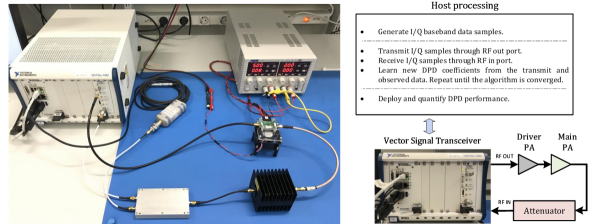
(a) RF measurement setup at FR-1.

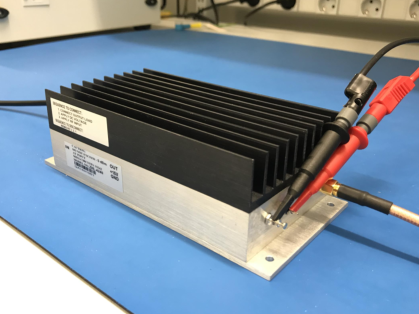
(b) General purpose wideband PA.

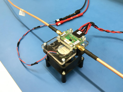
(c) Skyworks NR Band 78 PA.

Figure 4:  Overall RF measurement setup at FR-1 and the sub-6 GHz PA modules used in the Experiments 1-2.

The resulting exact numerical processing complexities, expressed in terms of real multiplications per linearized sample, are presented in Table II. In these numerical values, when it comes to the SPH and SMP DPD, we have excluded the trivial operations, i.e., multiplications by zeros, ones and integer powers of two or half, stemming from the structure of $\mathbf{B}_{3}$ in (11). Overall, the results in Table II demonstrate the large complexity reduction provided by the proposed spline-based DPD approaches, as nearly 64% (SPH) and 44% (SMP) less real multiplications per sample are needed in the DPD main path to predistort the input signal. Furthermore, the required parameter learning complexity is also very remarkably reduced, by approximately 95% in both SPH and SMP cases in terms of real multiplications per sample, indicating that solutions like these might already facilitate even continuous learning in selected applications. Additionally, owing to the largely reduced learning complexity, the feasibility of implementing both the DPD parameter learning as well as the main path processing in the same chip increases.

V Experimental Results

In order to evaluate and validate the proposed DPD concepts, three separate linearization experiments are carried out. Two of the measurement scenarios are related to FR-1 (sub-6 GHz) PAs and classical conducted measurements, including a general purpose wideband PA and a 5G NR Band 78 small-cell BS PA. The third experiment is then related to FR-2 and over-the-air (OTA) measurements where a state-of-the-art 28 GHz active antenna array with 64 integrated PAs and antenna units is linearized. For complexity assessment, we use the derived results in Table I, while again exclude the trivial operations, i.e., multiplications by zeros, ones and integer powers of two or half, stemming from the structure of the B-spline basis matrix $\mathbf{B}_{P_{\mathrm{SP}}}$. Additionally, we also provide the corresponding amounts of floating point operations (FLOPs) per sample. One complex multiplication is assumed to cost 6 FLOPs, while one complex-real multiplication and one complex sum both cost 2 FLOPs[40].

V-A FR-1 Measurement Environment and Figures of Merit

The FR-1 measurement setup utilized for the first two experiments is illustrated in Fig. 4(a), and consists of a National Instruments PXIe-5840 vector signal transceiver (VST), facilitating arbitrary waveform generation and analysis between 0–6 GHz with instantaneous bandwidth of 1 GHz. This instrument is used as both the transmitter and the observation receiver, and includes also an additional host-processing based computing environment where all the digital waveform and DPD processing can be executed. In a typical conducted measurement, the baseband complex I/Q waveform is generated by Matlab in the VST host environment, and fed to the device under test (DUT) through the VST transmit chain. The DUT output is then observed via the VST receiver, through an external attenuator. All DPD parameter learning and actual DPD main math processing stages are executed in the host environment. Finally, the actual DPD performance measurements are carried out where different random modulating data is used, compared to the learning phase.

As the DPD system figures of merit, we adopt the well-established error vector magnitude (EVM) and ACLR metrics, as defined for 5G NR in [23]. The EVM focuses on the passband transmit signal quality, and is defined as

$$\operatorname{EVM\;(\%)}=\sqrt{\frac{P_{\mathrm{error,\;eq.}}}{P_{\mathrm{ref.}}}}\times 100,$$ (34)

where $P_{\mathrm{error,\;eq.}}$ denotes the power of the error signal calculated between the ideal subcarrier symbols and the corresponding observed subcarrier samples at the PA output after zero forcing equalization removing the effects of the possible linear distortion [23]. Furthermore, $P_{\mathrm{ref.}}$ denotes the corresponding power of the ideal (reference) symbols. The ACLR, in turn, is defined as the ratio of the transmitted power within the desired channel ($P_{\mathrm{desired\;ch}}$) and that in the left or right adjacent channel ($P_{\mathrm{adj.\;ch.}}$), expressed as

$$\operatorname{ACLR\;(dB)}=10\operatorname{log_{10}}\frac{P_{\mathrm{desired\;ch.}}}{P_{\mathrm{adj.\;ch.}}},$$ (35)

measuring thus the out-of-band performance. While ACLR is, by definition, a relative measure, an explicit out-of-band spectral density limit, in terms of dBm/MHz measured with a sliding 1 MHz window in the adjacent channel region, is also defined for certain base-station types [23], referred to as the absolute basic limit in 3GPP terminology. Thus, the PA output spectral density in dBm/MHz is also quantified in the measurements, particularly in the context of local area and medium-range BS PAs [23].

All the forth-coming experiments utilize 5G NR Release-15 standard compliant OFDM downlink waveform and channel bandwidths [23], while the adopted carrier frequencies in each experiment are selected according to the available 5G NR bands and the available PA samples. In all experiments, the initial PAPR of the digital waveform is 9.5 dB, when measured at the 0.01% point of the instantaneous PAPR complementary cumulative distribution function (CCDF), and is then limited to 7 dB through well-known iterative clipping and filtering based processing, while also additional time-domain windowing is applied to suppress the inherent OFDM signal sidelobes. These impose an EVM floor of some 4% to the transmit signal. More specific waveform parameters such as the subcarrier spacing (SCS) and the occupied physical resource block (PRB) count are stated along the experiments.

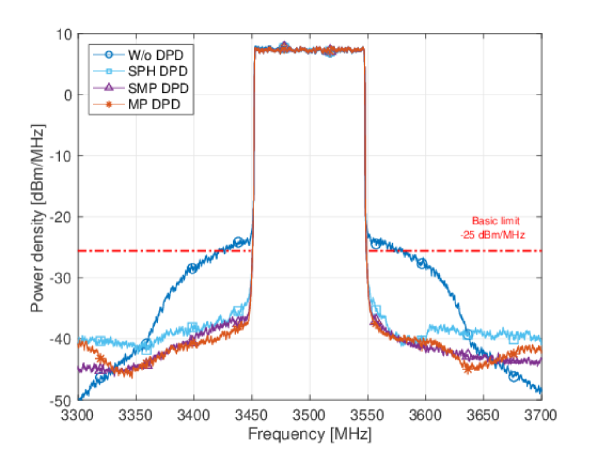
Figure 5:  Example illustration of linearization results in Experiment 1 (general purpose PA measured at 3.5 GHz), with 100 MHz channel bandwidth and PA output power of +27 dBm, while adopting $P_{\mathrm{SP}}=3$, $Q_{\mathrm{SPH}}=Q_{\mathrm{SMP}}=7$, $M_{\mathrm{SPH}}=3$, $M_{\mathrm{SMP}}=4$, $P_{\mathrm{MP}}=11$, and $M_{\mathrm{MP}}=4$.

V-B Experiment 1: General Purpose PA

The first experiment focuses on a general purpose wideband PA (Mini-Circuits ZHL-4240), illustrated in Fig. 4(b), as the actual amplification stage. The amplifier has a gain of 41 dB, and a 1-dB compression point of +31 dBm, being basically applicable in small-cell and medium-range base-stations. The transmit signal is a 5G NR downlink OFDM waveform, with 30 kHz subcarrier spacing and 264 active PRBs [23], yielding an aggressive passband width of 95.04 MHz. The RF center frequency is 3.5 GHz and the assumed channel bandwidth is 100 MHz. The I/Q samples are transmitted through the VST RF output port directly to the PA, facilitating a maximum output power of +27 dBm. The proposed and the reference DPD schemes are then adopted, and the performance quantification measurements are carried out. In all results, five ILA learning iterations are adopted while the signal length within each ILA iteration is 100,000 samples. In this experiment, the VST observation receiver runs at 491.52 MHz (4x oversampling).

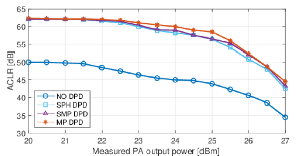
(a)

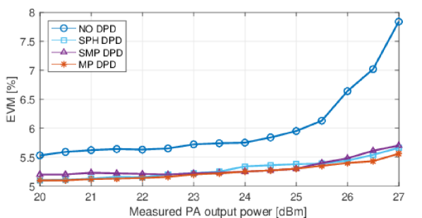
(b)

Figure 6:  Measured ACLR and EVM performance in Experiment 1 as a function of the PA output power, while adopting $P_{\mathrm{SP}}=3$, $Q_{\mathrm{SPH}}=Q_{\mathrm{SMP}}=7$, $M_{\mathrm{SPH}}=3$, $M_{\mathrm{SMP}}=4$, $P_{\mathrm{MP}}=11$, and $M_{\mathrm{MP}}=4$.

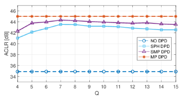
(a)

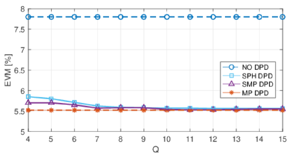
(b)

Figure 7:  Measured ACLR and EVM performance in Experiment 1 at PA output power of +27 dBm, as a function of the number of LUT control points in the SPH and SMP models, $Q$, while adopting $P_{\mathrm{SP}}=3$, $M_{\mathrm{SPH}}=3$, $M_{\mathrm{SMP}}=4$, $P_{\mathrm{MP}}=11$, and $M_{\mathrm{MP}}=4$.

Fig. 5 shows a snap-shot linearization example, at PA output power of +27 dBm, when $P_{\mathrm{SP}}=3$ is chosen as the spline order in both the SPH and SMP models, while the number of control points is fixed to $Q_{\mathrm{SPH}}=Q_{\mathrm{SMP}}=7$ and the memory filter orders are $M_{\mathrm{SPH}}=3$ and $M_{\mathrm{SMP}}=4$. Additionally, an LMS-based MP DPD of order $P_{\mathrm{MP}}=11$ with memory filters of order $M_{\mathrm{MP}}=4$ is also adopted and presented for reference. We can observe that the performances of the proposed SPH and SMP DPDs are very close to each other, and to that of the MP DPD, despite the substantially reduced complexity. The figure also illustrates that all DPD methods basically satisfy the absolute basic limit requirement of -25 dBm/MHz, which if less stringent than the classical 45 dB ACLR limit, and applies in medium-range BS cases with TX powers of higher than +24 dBm up to +38 dBm [23].

TABLE III: Summary of DPD main path processing complexity and linearization performance in Experiment 1, PA output power is +27 dBm

	Running complexity							Model performance
	P	M	Q	$\Delta_{z,x}$	# of coefficients	FLOPs/sample	Mul./sample	EVM (%)	Max. dBm/MHz
No DPD	-	-	-	-	-	-	-	7.82	-23.80
SPH DPD	2	3	7	1	12	55	28	5.61	-32.30
	3	3	7	1	13	69	36	5.54	-36.30
	4	3	7	1	14	89	45	5.55	-36.80
SMP DPD	2	4	7	1	30	65	50	5.55	-37.20
	3	4	7	1	31	99	63	5.57	-37.80
	4	4	7	1	32	143	77	5.57	-37.80
MP DPD	11	4	-	-	24	255	112	5.47	-38.20

Fig. 6 then presents the behavior of the measured EVM and ACLR performance metrics, as functions of the PA output power, following the same DPD parameterization. Again, we can observe that the proposed SPH, SMP, and the MP DPD behave very similarly. Similar type of observation follows also from Fig. 7, showing again the EVM and ACLR metrics but this time at fixed PA output power of +27 dBm while then varying the number of LUT control points in the proposed SPH and SMP models. From this figure we can also observe that the LUT based DPD performance is optimized with some $Q=7$ or $Q=8$ control points, in this example, while in general it is likely that the optimization of the value of $Q$ is to be done separately for different PA types.

Finally, Table III then collects and summarizes the obtained DPD results in Experiment 1 while also showing the DPD main path processing complexities. Here also other spline interpolation orders $P_{\mathrm{SP}}$ are considered and shown. We can conclude that the proposed spline-based DPD models offer a favorable performance-complexity trade-off compared to the reference MP DPD approach.

V-C Experiment 2: 5G NR Band 78 Small-Cell PA

TABLE IV: Summary of DPD main path processing complexity and linearization performance in Experiment 2, PA output power is +24 dBm

	Running complexity							Model performance
	P	M	Q	$\Delta_{z,x}$	# of coefficients	FLOPs/sample	Mul./sample	EVM (%)	Max. dBm/MHz
No DPD	-	-	-	-	-	-	-	8.64	-18.20
SPH DPD	2	4	7	1	13	63	32	5.70	-31.40
	3	4	7	1	14	77	40	5.57	-33.20
SMP DPD	2	5	7	1	37	73	56	5.60	-32.90
	3	5	7	1	38	111	75	5.55	-33.10
MP DPD	11	5	-	-	30	255	136	5.54	-33.20

The second experiment includes the Skyworks SKY66293-21 PA module, illustrated in Fig. 4(c), which is a low-to-medium power PA oriented to be used either in small-cell base-stations or in large antenna array transmitters. The PA module is specifically designed to operate in the NR Band n78 (3300-3800 MHz), having a gain of 34 dB, and a 1-dB compression point of +31.5 dBm. Similar 5G NR downlink signal corresponding to the 100 MHz channel bandwidth scenario, as in the Experiment 1, is adopted, while the considered RF center-frequency is 3.65 GHz. The test signal is again transmitted via the RF TX port of the VST directly to the PA module, while the considered PA output power is +24 dBm, corresponding to the maximum transmit power of a Local Area BS according to the NR regulations [23]. Again, five ILA learning iterations are adopted while the signal length within each ILA iteration is 100,000 samples. The VST observation receiver runs at 491.52 MHz (4x oversampling).

Fig. 8 and Table IV illustrate and summarize the obtained linearization results for the proposed and the reference DPD methods. Again, also comparative complexity numbers are stated in Table IV. As stated in [23], a 5G NR Local Area BS can operate within an absolute basic limit of -32 dBm/MHz in the adjacent channel region, assuming the considered PA output power of +24 dBm. As shown in Fig. 8 and Table IV, the SPH, SMP, and the MP DPD satisfy this limit, indicating successful linearization. Again, as can be observed in Table IV, a remarkable complexity reduction is obtained through the proposed spline-based DPD approaches, compared to the reference MP DPD, while all provide a very similar linearization performance.

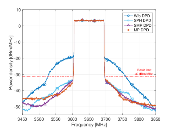
Figure 8:  Example illustration of linearization results in Experiment 2 (NR small-cell PA measured at 3.65 GHz), with 100 MHz channel bandwidth and PA output power of +24 dBm, while adopting $P_{\mathrm{SP}}=3$, $Q_{\mathrm{SPH}}=Q_{\mathrm{SMP}}=7$, $M_{\mathrm{SPH}}=4$, $M_{\mathrm{SMP}}=5$, $P_{\mathrm{MP}}=11$, and $M_{\mathrm{MP}}=5$.

V-D Experiment 3: FR-2 Environment and 28 GHz Active Array

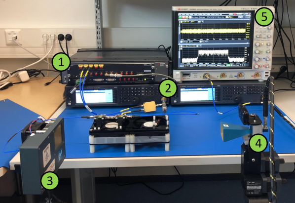
Figure 9:  RF measurement setup in Experiment 3 including the Keysight M8190 arbitrary waveform generator (1), Keysight N5183B-MXG LO signal generators (2), Anokiwave AWMF-0129 active antenna array (3) working at 28 GHz center frequency (NR Band n257), horn antenna as receiver (4), and Keysight DSOS804A digitizer (5).

In order to further demonstrate the applicability of the proposed spline-based DPD concepts, the third and final experiment focuses on timely 5G NR mmWave/FR-2 deployments [23] with active antenna arrays. Unwanted emission modeling and DPD-based linearization of active arrays with large numbers of PA units is, generally, an active research field, with good examples of recent papers being, e.g., [41, 42, 43, 5, 44, 45]. Below we first describe shortly the FR-2 measurement setup, and then present the actual linearization results.

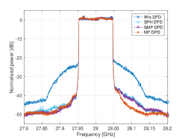
(a)

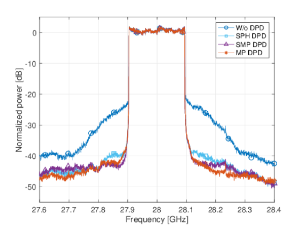
(b)

Figure 10:  Illustration of OTA linearization of the Anokiwave AWMF-0129 active antenna array, when (a) NR 100 MHz and (b) NR 200 MHz transmit signals are applied, measured at EIRP of +42.5 dBm The SPH and SMP DPD spline order is $P_{\mathrm{SP}}=3$, while $Q_{\mathrm{SPH}}=Q_{\mathrm{SMP}}=7$, $M_{\mathrm{SPH}}=3$, and $M_{\mathrm{SMP}}=4$. The MP DPD order is $P_{\mathrm{MP}}=11$ while $M_{\mathrm{MP}}=4$.

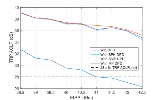
(a)

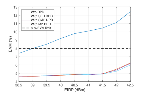
(b)

Figure 11:  OTA linearization performance of the Anokiwave AWMF-0129 active antenna array as a function of the EIRP of the proposed DPD models in terms of a) TRP ACLR, and b) EVM.

V-D1 FR-2 Measurement Setup

The overall mmWave/FR-2 measurement setup is depicted in Fig. 9, incorporating an Anokiwave AWMF-0129 active antenna array together with other relevant instruments and equipment for signal generation and analysis, facilitating measurements at 28 GHz center-frequency with up to 3 GHz of instantaneous bandwidth. On the transmit chain side, the setup consists of a Keysight M8190 arbitrary waveform generator that is used to generate directly the I/Q samples of a wideband modulated IF signal centered at 3.5 GHz. The signal is then upconverted to the 28 GHz carrier frequency by utilizing the Keysight N5183B-MXG that generates the corresponding local oscillator signal running at 24.5 GHz, together with external mixers and filters. The modulated RF waveform is then pre-amplified by means of two Analog Devices’ driver PAs, HMC499LC4 and HMC943ALP5DE, with 17 dB and 23 dB gain, respectively, such that the integrated PAs of the Anokiwave AWMF-0129 active antenna array are driven towards saturation.

The transmit signal propagates over-the-air (OTA) and is captured by a horn antenna at the observation receiver, such that the receiving antenna system is well aligned with the main transmit beam. At the receiver side, another Keysight N5183B-MXG and a mixing stage are used to downconvert the signal back to IF. Then, the Keysight DSOS804A oscilloscope is utilized as the actual digitizer, including also built-in filtering, and the signal is taken to baseband and processed in a host PC, where the DPD learning and predistortion are executed. The OTA measurement system is basically following the measurement procedures described in [23, 46], specifically the measurement option utilizing the beam-based directions. In these measurements, the observation receiver provides I/Q samples at 7x oversampled rate.

TABLE V: Summary of linearization performance of the Anokiwave AWMF-0129 active antenna array, with 100 MHz and 200 MHz 5G NR channel bandwidths, measured at +42.5 dBm EIRP

	DPD running complexity						DPD perf., 100 MHz		DPD perf., 200 MHz
	P	M	Q	$\Delta_{z,x}$	FLOPs/sample	Mul./sample	EVM (%)	TRP ACLR (dB)	EVM (%)	TRP ACLR (dB)
No DPD	-	-	-	-	0	0	12.10	26.10	12.43	26.30
SPH DPD	3	3	7	1	69	36	6.20	34.40	6.25	34.10
SMP DPD	3	4	7	1	99	63	6.15	34.80	6.20	34.40
MP DPD	11	4	-	-	255	112	6.00	35.20	6.13	35.00

V-D2 Active Array Linearization

Linearization of active phased-array transmitters is generally a challenging task, since a single DPD unit must linearize a bank of mutually different PAs. There are multiple ways of acquiring the observation signal for DPD parameter learning, as discussed e.g. in [42, 5, 43, 45, 44]. In this work, we assume and adopt the so-called combined observation signal approach and utilize specifically the OTA-combined received signal for DPD parameter learning [42, 5, 45], while otherwise following exactly the same learning algorithms as in the Experiments 1 and 2.

In the DPD measurements, we adopt 5G NR FR-2 OFDM signal with SCS of 60 kHz, and consider active PRB counts of 132 and 264, mapping to 100 MHz and 200 MHz channel bandwidths, respectively [23]. In this case, 5 ILA iterations are adopted, each containing 50,000 samples. Example OTA linearization results are illustrated in Fig. 10, measured at an EIRP of +42.5 dBm, where the received spectra with the proposed SPH, SMP and the reference MP DPD are shown, while the no-DPD case is also shown for comparison. The parametrization of the SPH and SMP DPD is $P_{\mathrm{SP}}=3$ and $M_{\mathrm{SPH}}=3$, and $M_{\mathrm{SMP}}=4$, while MP DPD is configured with $P_{\mathrm{MP}}=11$ and $M_{\mathrm{MP}}=4$. As mentioned already in the introduction, the OTA ACLR requirements at FR-2 are quite clearly relaxed, compared to the classical 45 dB number at FR-1, with 28 dB defined as the TRP-based ACLR limit in the current NR Release-15 specifications [23]. Additionally, 64-QAM is currently the highest supported modulation scheme at FR-2, heaving 8% as the required EVM.

In both channel bandwidth cases, considered in Fig. 10, the initial EVM and TRP ACLR metrics are around 12.5% and 26 dB, respectively, when measuring at EIRP of +42.5 dBm and when no DPD is applied. Hence, linearization is indeed required if the same output power is to be maintained, while Fig. 10 demonstrates that all considered DPD methods can successfully linearize the active array. Table V shows the exact measured numerical TRP ACLR and EVM values, indicating good amounts of linearization gain and that the EVM and TRP ACLR requirements can be successfully met. It is also noted that the initial TRP ACLR of some 26 dB corresponds already to a very nonlinear starting point.

Finally, Fig. 11 features a power sweep performed with the antenna array, illustrating the TRP ACLR and EVM as a function of the EIRP with and without DPD. It can be clearly observed that in this particular experiment, when no DPD is applied, it is the EVM metric that is limiting the maximum achievable EIRP such that both TRP ACLR and EVM requirements are still fulfilled. Specifically, without DPD processing, this limits the maximum EIRP to some +39 dBm, while when DPD processing is applied, both requirements are fulfilled at least up to the considered maximum EIRP of +42.5 dBm – and clearly also somewhat beyond. In this particular linearization experiment, it can be noted that the SPH DPD is an intriguing approach, due to its very low computational complexity, while still being clearly able to linearize the array.

VI Conclusions

In this paper, novel complex spline-interpolated LUT concepts and corresponding DPD methods with gradient-adpative learning rules were proposed for power amplifier linearization. A vast amount of different measurement-based experiments were provided, covering successful linearization of different PA samples at sub-6 GHz bands. Additionally, a 28 GHz state-of-the-art active antenna array was successfully linearized. The measured linearization performance results, together with the provided explicit complexity analysis, show that the proposed spline-interpolated DPD concepts can provide very appealing complexity-performance trade-offs, compared to, e.g., ordinary canonical MP DPD. Specifically, the SMP DPD was shown to provide in all measurement examples linearization performance very close to that of ordinary MP DPD, while having substantially lower main path and DPD learning complexity. Additionally, the SPH DPD offers further reduction in the main path processing complexity, while was also shown to be performing fairly close to the other DPD systems, particularly in the timely 28 GHz active array linearization experiment.

Pablo Pascual Campo received his B.Sc. and M.Sc. degrees in Telecommunications and Electrical Engineering in 2012 and 2014, respectively, from Universidad Politécnica de Madrid, Madrid, Spain. He is currently pursuing his D.Sc. degree at Tampere University, Department of Electrical Engineering, Tampere, Finland. His research interests include digital predistortion, full-duplex systems and applications, and signal processing for wireless communications at the mmWave bands.

Alberto Brihuega (S’18) received the B.Sc. and M.Sc. degrees in Telecommunications Engineering from Universidad Politécnica de Madrid, Spain, in 2015 and 2017, respectively. He is currently working towards the Ph.D. degree with Tampere University, Finland, where he is a researcher with the Department of Electrical Engineering. His research interests include statistical and adaptive digital signal processing for compensation of hardware impairments in large-array antenna transceivers.

Lauri Anttila received the D.Sc. (Tech.) degree (with distinction) in 2011 from Tampere University of Technology (TUT), Finland. Since 2016, he has been a University Researcher at the Department of Electrical Engineering, Tampere University (formerly TUT). In 2016-2017, he was a Visiting Research Fellow at the Department of Electronics and Nanoengineering, Aalto University, Finland. His research interests are in radio communications and signal processing, with a focus on the radio implementation challenges in systems such as 5G, full-duplex radio, and large-scale antenna systems.

Matias Turunen is currently pursuing the M.Sc. degree in electrical engineering at Tampere University (TAU), Tampere, Finland, while also working as a Research Assistant with the Department of Electrical Engineering at TAU. His current research interests include in-band full-duplex radios with an emphasis on analog RF cancellation, OFDM radar, and 5G New Radio systems.

Dani Korpi received D.Sc. degree (Hons.) in electrical engineering from Tampere University of Technology, Finland, in 2017. Currently, he is a Senior Specialist with Nokia Bell Labs in Espoo, Finland. His doctoral thesis received an award for the best dissertation of the year in Tampere University of Technology, as well as the Finnish Technical Sector’s Award for the best doctoral dissertation of 2017. His research interests include inband full-duplex radios, machine learning for wireless communications, and beyond 5G radio systems.

Markus Allén received the B.Sc., M.Sc. and D.Sc. degrees in communications engineering from Tampere University of Technology, Finland, in 2008, 2010 and 2015, respectively. He is currently with the Department of Electrical Engineering at Tampere University, Finland, as a University Instructor. His current research interests include software-defined radios, 5G-related RF measurements and digital signal processing for radio transceiver linearization.

Mikko Valkama received the D.Sc. (Tech.) degree (with honors) in electrical engineering from Tampere University of Technology (TUT), Finland, in 2001. In 2003, he was a visiting post-doc research fellow with SDSU, San Diego, CA. Currently, he is a Full Professor and Department Head of Electrical Engineering at the newly formed Tampere University (TAU), Finland. His research interests include radio communications, radio localization, and radio-based sensing, with particular emphasis on 5G and beyond mobile radio networks.

References

- [1] E. Dahlman, S. Parkvall, and J. Skold, 5G NR: The Next Generation Wireless Access Technology, 1st ed. Academic Press, 2018.
- [2] F. M. Ghannouchi and O. Hammi, “Behavioral modeling and predistortion,” IEEE Microw. Mag., vol. 10, no. 7, pp. 52–64, Dec. 2009.
- [3] Y. Rahmatallah and S. Mohan, “Peak-to-average power ratio reduction in OFDM systems: A survey and taxonomy,” IEEE Commun. Surveys Tuts., vol. 15, no. 4, pp. 1567–1592, Mar. 2013.
- [4] S. Afsardoost, T. Eriksson, and C. Fager, “Digital predistortion using a vector-switched model,” IEEE Trans. Microw. Theory Tech., vol. 60, no. 4, pp. 1166–1174, April 2012.
- [5] C. Fager et al., “Linearity and efficiency in 5G transmitters: New techniques for analyzing efficiency, linearity, and linearization in a 5G active antenna transmitter context,” IEEE Microw. Mag., vol. 20, no. 5, pp. 35–49, May 2019.
- [6] O. Hammi, F. M. Ghannouchi, and B. Vassilakis, “A compact envelope-memory polynomial for RF transmitters modeling with application to baseband and RF-digital predistortion,” IEEE Microw. Wireless Compon. Lett., vol. 18, no. 5, pp. 359–361, May 2008.
- [7] M. Abdelaziz, L. Anttila, A. Kiayani, and M. Valkama, “Decorrelation-based concurrent digital predistortion with a single feedback path,” IEEE Trans. Microw. Theory Tech., vol. 66, no. 1, pp. 280–293, Jan. 2018.
- [8] Y. Ma, Y. Yamao, Y. Akaiwa, and C. Yu, “FPGA implementation of adaptive digital predistorter with fast convergence rate and low complexity for multi-channel transmitters,” IEEE Trans. Microw. Theory Tech., vol. 61, no. 11, pp. 3961–3973, Nov 2013.
- [9] J. Kim and K. Konstantinou, “Digital predistortion of wideband signals based on power amplifier model with memory,” Electron. Lett., vol. 37, no. 23, p. 1, Nov. 2001.
- [10] A. Zhu, “Digital predistortion and its combination with crest factor reduction,” in Digital Front-End in Wireless Communications and Broadcasting: Circuits and Signal Processing, F.-L. Luo, Ed. Cambridge: Cambridge University Press, 2011, ch. 9, pp. 244–279.
- [11] A. S. Tehrani et al., “A comparative analysis of the complexity/accuracy tradeoff in power amplifier behavioral models,” IEEE Trans. Microw. Theory Tech., vol. 58, no. 6, pp. 1510–1520, June 2010.
- [12] D. R. Morgan, Z. Ma, J. Kim, M. G. Zierdt, and J. Pastalan, “A generalized memory polynomial model for digital predistortion of RF power amplifiers,” IEEE Trans. Signal Process., vol. 54, no. 10, pp. 3852–3860, Oct. 2006.
- [13] F. Mkadem, A. Islam, and S. Boumaiza, “Multi-band complexity-reduced generalized-memory-polynomial power-amplifier digital predistortion,” IEEE Trans. Microw. Theory Tech., vol. 64, no. 6, pp. 1763–1774, June 2016.
- [14] A. Zhu and T. J. Brazil, “An overview of volterra series based behavioral modeling of RF/microwave power amplifiers,” in 2006 IEEE Annual Wireless and Microwave Technology Conference, Dec. 2006, pp. 1–5.
- [15] ——, “Behavioral modeling of RF power amplifiers based on pruned volterra series,” IEEE Microw. Wireless Compon. Lett., vol. 14, no. 12, pp. 563–565, Dec. 2004.
- [16] M. Schetzen, The Volterra and Wiener Theories of Nonlinear Systems. Melbourne, FL, USA: Krieger Publishing Co., Inc., 2006.
- [17] C. Yu, L. Guan, E. Zhu, and A. Zhu, “Band-limited volterra series-based digital predistortion for wideband RF power amplifiers,” IEEE Trans. Microw. Theory Tech., vol. 60, no. 12, pp. 4198–4208, Dec. 2012.
- [18] N. Safari, N. Holte, and T. Roste, “Digital predistortion of power amplifiers based on spline approximations of the amplifier characteristics,” in 2007 IEEE 66th Veh. Technol. Conf., Sep. 2007, pp. 2075–2080.
- [19] N. Safari, P. Fedorenko, J. S. Kenney, and T. Roste, “Spline-based model for digital predistortion of wide-band signals for high power amplifier linearization,” in 2007 IEEE/MTT-S International Microwave Symposium, June 2007, pp. 1441–1444.
- [20] J. Kral, T. Gotthans, R. Marsalek, M. Harvanek, and M. Rupp, “On feedback sample selection methods allowing lightweight digital predistorter adaptation,” IEEE Trans. Circuits Syst. I, vol. 67, no. 6, June 2020.
- [21] C. Cheang, P. Mak, and R. P. Martins, “A hardware-efficient feedback polynomial topology for dpd linearization of power amplifiers: Theory and fpga validation,” IEEE Trans. Circuits Syst. I, vol. 65, no. 9, pp. 2889–2902, 2018.
- [22] F. M. Barradas, T. R. Cunha, P. M. Lavrador, and J. C. Pedro, “Polynomials and LUTs in PA behavioral modeling: A fair theoretical comparison,” IEEE Trans. Microw. Theory Tech., vol. 62, no. 12, pp. 3274–3285, Nov. 2014.
- [23] 3GPP Tech. Spec. 38.104, “NR; Base Station (BS) radio transmission and reception,” v15.4.0 (Release 15), Dec. 2018.
- [24] K.-F. Liang, J.-H. Chen, and Y.-J. E. Chen, “A quadratic-interpolated LUT-based digital predistortion technique for cellular power amplifiers,” IEEE Trans. Circuits Syst. II, vol. 61, no. 3, pp. 133–137, Mar. 2014.
- [25] A. Molina, K. Rajamani, and K. Azadet, “Digital predistortion using lookup tables with linear interpolation and extrapolation: Direct least squares coefficient adaptation,” IEEE Trans. Microw. Theory Tech., vol. 65, no. 3, pp. 980–987, Nov. 2017.
- [26] P. Jardin and G. Baudoin, “Filter lookup table method for power amplifier linearization,” IEEE Trans. Veh. Technol., vol. 56, no. 3, pp. 1076–1087, May 2007.
- [27] X. Wu, N. Zheng, X. Yang, J. Shi, and H. Chen, “A spline-based hammerstein predistortion for 3G power amplifiers with hard nonlinearities,” in 2010 2nd Int. Conf. Future Comp. Commun., vol. 3, May 2010.
- [28] O. Hammi, F. M. Ghannouchi, S. Boumaiza, and B. Vassilakis, “A data-based nested LUT model for RF power amplifiers exhibiting memory effects,” IEEE Microw. Wireless Compon. Lett., vol. 17, no. 10, pp. 712–714, Oct. 2007.
- [29] H. Zhi-yong et al., “An improved look-up table predistortion technique for HPA with memory effects in OFDM systems,” IEEE Trans. Broadcasting, vol. 52, no. 1, pp. 87–91, Feb. 2006.
- [30] Z. Wang et al., “Low computational complexity digital predistortion based on direct learning with covariance matrix,” IEEE Trans. Microw. Theory Tech., vol. 65, no. 11, pp. 4274–4284, May 2017.
- [31] C. De Boor, A Practical Guide to Splines. Springer, New York, 1978.
- [32] M. Scarpiniti, D. Comminiello, R. Parisi, and A. Uncini, “Nonlinear spline adaptive filtering,” Signal Process., vol. 93, no. 4, pp. 772–783, Apr. 2013.
- [33] ——, “Hammerstein uniform cubic spline adaptive filters: Learning and convergence properties,” Signal Process., vol. 100, pp. 112–123, July 2014.
- [34] ——, “Novel cascade spline architectures for the identification of nonlinear systems,” IEEE Trans. Circuits Syst. I, vol. 62, no. 7, pp. 1825–1835, July 2015.
- [35] S. Haykin, Adaptive Filter Theory. Prentice Hall, 2001.
- [36] D. H. Brandwood, “A complex gradient operator and its application in adaptive array theory,” IEE Proceedings F - Commun., Radar and Signal Process., vol. 130, no. 1, pp. 11–16, Feb. 1983.
- [37] M. Frerking, Digital Signal Processing in Communications Systems. Springer, 1994.
- [38] R. Raich, Hua Qian, and G. T. Zhou, “Orthogonal polynomials for power amplifier modeling and predistorter design,” IEEE Trans. Veh. Technol., vol. 53, no. 5, pp. 1468–1479, Sep. 2004.
- [39] R. Dallinger, H. Ruotsalainen, R. Wichman, and M. Rupp, “Adaptive pre-distortion techniques based on orthogonal polynomials,” in 44th Asilomar Conf. Signals, Syst., and Computers, 2010, pp. 1945–1950.
- [40] R. J. Schilling and S. L. Harris, Fundamentals of Digital Signal Processing Using MATLAB. Cengage Learning, 2010.
- [41] C. Mollen, E. G. Larsson, U. Gustavsson, T. Eriksson, and R. W. Heath, “Out-of-band radiation from large antenna arrays,” IEEE Commun. Mag., vol. 56, no. 4, pp. 196–203, April 2018.
- [42] M. Abdelaziz, L. Anttila, A. Brihuega, F. Tufvesson, and M. Valkama, “Digital Predistortion for Hybrid MIMO Transmitters,” IEEE J. Sel. Topics Signal Process., vol. 12, no. 3, pp. 445–454, June 2018.
- [43] A. Brihuega, L. Anttila, M. Abdelaziz, and M. Valkama, “Digital Predistortion in Large-Array Digital Beamforming Transmitters,” in 52nd Asilomar Conf. Signals, Syst., Comp., Oct. 2018, pp. 611–618.
- [44] X. Liu, Q. Zhang, W. Chen, H. Feng, L. Chen, F. M. Ghannouchi, and Z. Feng, “Beam-Oriented Digital Predistortion for 5G Massive MIMO Hybrid Beamforming Transmitters,” IEEE Trans. Microw. Theory Tech., vol. 66, no. 7, pp. 3419–3432, July 2018.
- [45] N. Tervo et al., “Digital predistortion of amplitude varying phased array utilising over-the-air combining,” in 2017 IEEE MTT-S International Microwave Symposium (IMS), June 2017, pp. 1165–1168.
- [46] 3GPP Tech. Spec. 38.141-2, “NR; Base Station (BS) conformance testing, Part 2,” v15.1.0 (Release 15), March 2019.