Randomized sequential importance sampling for estimating the number of perfect matchings in bipartite graphs

Abstract.

We introduce and study randomized sequential importance sampling algorithms for estimating the number of perfect matchings in bipartite graphs. In analyzing their performance, we establish various non-standard central limit theorems. We expect our methods to be useful for other applied problems.

1. Introduction

Sequential importance sampling is a widely used technique for Monte Carlo evaluation of intractable counting and statistical problems. Using randomized algorithms, we apply this method to estimate the number of perfect matchings in bipartite graphs for a suite of test problems [16] where careful analytics can be carried out. We think that our techniques should be useful for estimating the number of perfect matchings in other types of bipartite graphs, and also for a variety of applied problems, such as counting and testing for contingency tables [10] and for graphs with given degree sequence [5].

Importance sampling uses a relatively simple measure $\mu$ to obtain information about a more complicated measure $\nu\ll\mu$ of interest. The Kullback–Leibler divergence $L={\bf E}_{\nu}\log(d\nu/d\mu)$ relates the two. Recent work [9] (see Section 2.2) shows that, if $\log(d\nu/d\mu)$ is concentrated, roughly $e^{L}$ samples from $\mu$ are necessary and sufficient to well approximate quantities of the form $\int fd\nu$.

In this work, $\mu$ is the uniform measure on the set of perfect matchings of a given graph, and $\nu$ is some other measure on this set induced by a randomized sampling algorithm. This work is the first to prove limit theorems for $\log(d\nu/d\mu)$ for a variety of graphs and algorithms, and thereby accurately gauge the efficiency of importance sampling in this context. Even for simple graphs and natural sampling algorithms, this turns out to be quite a non-standard problem.

Typically $L\sim cn$ is asymptotically linear, resulting in algorithms with exponential running times. However, the constants $c$ involved are small enough so that, for $n$ of practical interest, accurate estimates of huge numbers are available using reasonably small sample sizes. Indeed, our algorithms compare well with polynomial Markov chain Monte Carlo algorithms [21, 17, 4] within this range of $n$.

1.1. Setup

Suppose that $B_{n}$ is a bipartite graph on vertex sets $U_{n}=\{u_{1},\ldots,u_{n}\}$ and $V_{n}=\{v_{1},\ldots,v_{n}\}$ with various edges between them. Let ${\mathcal{M}}_{n}$ be the set of perfect matchings in $B_{n}$, supposing here and throughout that ${\mathcal{M}}_{n}\neq\emptyset$. We identify a perfect matching in ${\mathcal{M}}_{n}$ with the permutation $\pi\in S_{n}$ such that $\pi(i)=j$ if $u_{i}$ and $v_{j}$ are matched (and so speak of perfect matchings and permutations interchangeably).

In a variety of statistical problems arising with censored or truncated data it is important to understand the distribution of various statistics, e.g., the number of involutions, cycles or fixed points of uniformly distributed elements of ${\mathcal{M}}_{n}$. For example, Efron and Petrosian [18] need random matchings in a bipartite graph arising in an astrophysics problem; see [16] for discussion on how many such matchings are required in tests for parapsychology. These are provably $\#{\rm P}$-complete problems, so approximation is all that can be hoped for. See Section 2.1 for further discussion on matching theory.

Figure 1. A bipartite graph and its three perfect matchings.

Importance sampling, selects $\pi\in{\mathcal{M}}_{n}$ according to a distribution $P(\pi)$ which is relatively easy to sample from. For instance, consider the case that vertices in $U_{n}$ are matched in the fixed order $u_{1},u_{2},\ldots,u_{n}$, where in the $i$th step $u_{i}$ is matched with a vertex $v\in V_{n}$ uniformly at random amongst the remaining allowable options. Then $P(\pi)=\prod_{i}|I_{i}|^{-1}$, where $I_{i}(\pi)\subset V_{n}$ is the set of vertices $v\in V_{n}$ which (a) are not matched with any of $u_{1},u_{2},\ldots,u_{i-1}$ and (b) such that if next $u_{i}$ is matched with $v$ then it would still be possible to complete what remains to a perfect matching.

For example, the graph in Figure 1 has three perfect matchings $\pi_{1}=12534$, $\pi_{2}=12543$ and $\pi_{3}=24153$. Under the algorithm described in the previous paragraph, $P(\pi_{1})=1/4$, $P(\pi_{2})=1/4$ and $P(\pi_{3})=1/2$. To see this, note that $u_{1}$ can be matched with either $v_{1}$ or $v_{2}$. In the former case, $u_{2}$ must be matched with $v_{2}$, and then $u_{3}$ must be matched with $v_{5}$, and then finally $u_{4}$ can then be matched with either $v_{3}$ or $v_{4}$ (and then $u_{5}$ is matched with whichever of $v_{3}$ and $v_{4}$ remains to complete the matching). In the latter case, once $u_{1}$ is matched with $v_{2}$, the rest of the matching is forced, as then there is only one way to complete to a perfect matching.

The first key observation is that, letting $M_{n}=|{\mathcal{M}}_{n}|$ and $T(\pi)=P(\pi)^{-1}$, we have

$${\bf E}T(\pi)=\sum_{\pi}T(\pi)P(\pi)=M_{n},$$

so $T(\pi)$ is an unbiased estimator of $M_{n}$. Moreover, if $\pi_{1},\ldots,\pi_{N}$ is a sample from $P(\pi)$ then

$${\bf P}_{u}(Q(\pi)\leq\gamma_{2})\doteq\frac{1}{N}\sum_{i=1}^{N}\delta(Q(\pi_{i})\leq\gamma_{2})T(\pi_{i}),$$

where on the left, $Q(\pi)$ is a statistic of interest and $u=1/M_{n}$ is the uniform distribution on ${\mathcal{M}}_{n}$.

As already mentioned, recent work [9] suggests that in many cases a sample of size $N\doteq e^{L}$ is necessary and sufficient to well approximate $M_{n}$ by an importance sampling algorithm, where $L={\bf E}_{u}\log(T(\pi)/M_{n})$ is the Kullback–Leibler divergence of the importance sampling measure $P(\pi)$ from the uniform measure $u=1/M_{n}$ on ${\mathcal{M}}_{n}$. To apply this result, one needs to verify that $\log T(\pi)$ under $u$ is concentrated about its mean. See Section 2.2 for more details.

1.2. Results

Our main focus is the the test case of Fibonacci matchings

$${\mathcal{F}}_{n,1}=\{\pi\in S_{n}:|\pi(i)-i|\leq 1\}.$$

Our techniques also extend to other related classes of graphs introduced in [16], such as $t$-Fibonacci matchings

$${\mathcal{F}}_{n,t}=\{\pi\in S_{n}:-1\leq\pi(i)-i\leq t\},$$

and distance-$d$ matchings

$${\mathcal{D}}_{n,d}=\{\pi\in S_{n}:|\pi(i)-i|\leq d\}.$$

Figure 2. The 5 Fibonacci matchings of size $n=4$.

For simplicity, we restrict ourselves for the time being to the Fibonacci case. The reason for the name is that $F_{n,1}=|{\mathcal{F}}_{n,1}|$ is equal to the Fibonacci number $F_{n+1}$, as is easily seen by considering whether $\pi(1)=1$ or $\pi(1)=2$ (in which case necessarily $\pi(2)=1$). Although the size of ${\mathcal{F}}_{n,1}$ is known, our aim is to estimate $F_{n,1}$ by various importance sampling algorithms, so as to obtain a benchmark for its performance and to gain insight towards applying these methods in more complicated situations, in practice and theory.

For example, when $n=4$, there are 5 Fibonacci matchings. Two distributions $P_{1}$ and $P_{2}$ are listed below, corresponding to proceeding in orders $1,2,3,4$ and $2,3,1,4$, in each step matching $i$ at random amongst its neighbors whose matchings are yet to be determined. For instance $P_{1}(1234)=1/8$, since 1 can be matched with 1 or 2; then given $\pi(1)=1$, 2 can be matched with 2 or 3; then given $\pi(12)=12$, 3 can be matched with 3 or 4, and then $\pi(4)=4$ is forced. Similarly $P_{2}(1324)=1/3$, since $2$ can be matched with 1, 2 or 3; then given $\pi(2)=3$, the rest of $\pi$ is forced.

Table 1. Two schemes for Fibonacci matchings ${\mathcal{F}}_{4,1}$.

$\pi$	1234	2134	1324	1243	2143
$P_{1}(\pi)$	$1/8$	$1/4$	$1/4$	$1/8$	$1/4$
$P_{2}(\pi)$	$1/6$	$1/6$	$1/3$	$1/6$	$1/6$

A natural question to ask is how accurately can one estimate $F_{n,1}$ by an importance sampling algorithm ${\tt A}$ which in each step matches the current index $i$ with another index uniformly at random (amongst the remaining allowable options). We consider three such algorithms ${\tt A}_{r}$, ${\tt A}_{f}$ and ${\tt A}_{g}$ which match indices $[n]$ in uniformly random order, the fixed order $1,2,\ldots,n$, and according to a certain greedy order. In each step of ${\tt A}_{g}$ the smallest unmatched index $i$ is matched amongst those indices $i$ with the maximal number of remaining choices for $\pi(i)$. For instance, if in the first step of the algorithm 2 is matched with 1 or 2 (in which case $\pi(12)$ is determined), then 4 is matched in the next step; whereas if 2 is matched with 3 (in which case $\pi(123)$ is determined), then 5 is matched in the next step.

To analyze the performance of these algorithms, we prove the following central limit theorems.

Theorem 1.1.

Consider the distributions $P_{r}(\pi)$, $P_{f}(\pi)$ and $P_{g}(\pi)$ on Fibonacci matchings $\pi\in{\mathcal{F}}_{n,1}$ obtained by algorithms ${\tt A}_{r}$, ${\tt A}_{f}$ and ${\tt A}_{g}$, which in random, fixed and greedy orders (as above), sequentially match indices randomly amongst the remaining allowable options. Then, under the uniform measure $u=1/F_{n,1}$,

$$\frac{\log T_{r}(\pi)-\mu_{r}n}{\sigma_{r}\sqrt{n}},\quad\frac{\log T_{f}(\pi)-\mu_{f}n}{\sigma_{f}\sqrt{n}},\quad\frac{\log T_{g}(\pi)-\mu_{g}n}{\sigma_{g}\sqrt{n}}$$

all converge in distribution to standard normals $N(0,1)$, where

$$\mu_{r}\doteq 0.4944,\quad\mu_{f}\doteq 0.5016,\quad\mu_{g}\doteq 0.4913,$$

$$\sigma^{2}_{r}\doteq 0.0267,\quad\sigma^{2}_{f}\doteq 0.0430,\quad\sigma_{g}^{2}\doteq 0.0195.$$

See Theorems 3.2, 3.4 and 3.5 below for the precise values of $\mu$ and $\sigma^{2}$. Using [9] discussed above, we find that about $N^{*}=e^{\mu n+\sigma\sqrt{n}}/F_{n,1}$ samples are sufficient to well approximate $F_{n,1}$. For example, only about 194, 1520 and 75 samples are required for $F_{200,1}\doteq 4.5397\times 10^{41}$ by algorithms ${\tt A}_{r}$, ${\tt A}_{f}$ and ${\tt A}_{g}$. See Section 3.7 for more data.

In particular, we verify a conjecture of Don Knuth [22] that about $e^{c_{r}n+O(\sqrt{n})}$, where $c_{r}\doteq 0.013$, samples are needed to approximate $F_{n,1}$ using ${\tt A}_{r}$. Indeed, by Theorem 3.2, and since $F_{n,1}\sim\varphi^{n+1}/\sqrt{5}$, where $\varphi=(1+\sqrt{5})/2$, we find

$$c_{r}=\frac{1}{5}(\frac{13}{6}-\frac{2}{\sqrt{5}})\log{2}+\frac{1}{5}(1+\frac{1}{\sqrt{5}})\log{3}-\log\varphi\doteq 0.013143.$$

1.3. Discussion

We conclude with a series of remarks.

1.3.1. Comparing algorithms

By the results above we see that, in the case of Fibonacci matchings, the random order algorithm ${\tt A}_{r}$ performs significantly better than ${\tt A}_{f}$, which matches “from the top.” This was not clear to us at the outset, and was an early motivating question. It would appear that the reason for this is that typically in several steps of ${\tt A}_{r}$ there are three choices for $\pi(i)$, whereas in ${\tt A}_{f}$ there are only ever at most two. The greedy algorithm ${\tt A}_{g}$ capitalizes on this, and outperforms the others. Note that, although the means $\mu_{r}$, $\mu_{f}$ and $\mu_{g}$ are roughly comparable, the variances $\sigma_{r}^{2}$, $\sigma_{f}^{2}$ and $\sigma_{g}^{2}$ differ significantly.

The intuition behind ${\tt A}_{g}$ (sequentially matching the nearest unmatched vertex amongst those of largest degree) may lead to useful strategies for other classes of matchings, or other similar combinatorial tasks (where, depending on the situation, “largest degree” might be replaced with e.g. “most spead out choice”).

1.3.2. Exponential running times

Further to the exponential running times of our algorithms, we mention here that we also consider variants in Section 3.5 which make non-uniform decisions about how to match indices. Such non-uniform choices are crucial in the application of sequential importance sampling to estimating the number of contingency tables with fixed row/column sums [10] or the number of graphs with a given degree sequence [5]. The present paper gives the first set of cases where such improvements can be proved.

More specifically, we find “almost perfect” versions ${\tt A}^{*}$, for which $\mathrm{Var}_{u}T(\pi)=O(1)$. Such algorithms require only $O(1)$ samples to well approximate $F_{n,1}$. For example, in the case of the fixed order algorithm ${\tt A}_{f}$, we obtain ${\tt A}_{f}^{*}$ by in step $i$ setting $\pi(i)=i$ with probability $1/\varphi$ and $\pi(i)=i+1$ with probability $1/\varphi^{2}$ (unless in the previous step $\pi(i-1)=i$, in which case the matching $\pi(i)=i-1$ is forced). Recall that $F_{n,1}\sim\varphi^{n+1}/\sqrt{5}$, so $1/\varphi$ and $1/\varphi^{2}$ are the asymptotic proportions of Fibonacci matchings with $\pi(1)=1$ and $\pi(1)=2$. The optimal probabilities for other “almost perfect” algorithms ${\tt A}^{*}$ are found by similar considerations.

Of course, in these examples we have used the asymptotics of $F_{n,1}$, which in practice we would instead be attempting to approximate. Nonetheless, these observations suggest that adaptive versions of our algorithms (using e.g. the cross-entropy method [13]) might achieve sub-exponential running times.

1.3.3. CLTs for random order

Although Fibonacci matchings ${\mathcal{F}}_{n,1}$ and the random matching scheme ${\tt A}_{r}$ are quite simple and natural, we do not see a clear way of proving a central limit theorem for ${\tt A}_{r}$ by standard techniques. Instead, we apply the theory of Neininger and Rüschendorf [29] for probabilistic recurrences associated with randomized divide-and-conquer algorithms, often occurring in computer science contexts. This work develops an observation of Pittel [30] that random combinatorial structures with “nearly linear” mean and variance, and a recurrence for the associated moment generating functions, are often asymptotically normal. These methods may be useful for analyzing the performance of importance sampling algorithms in other applications.

The main difficulty in proving versions of Theorem 1.1 for ${\tt A}_{r}$ on matchings in ${\mathcal{F}}_{n,t}$ and ${\mathcal{D}}_{n,d}$, more generally, is calculating the mean and variance of $\log T_{r}(\pi)$. The computations become quite involved. The theory of [29] on the other hand is considerably robust.

1.3.4. Related works

Importance sampling was recently applied to Fibonacci and related matchings in [11]. This work takes a combinatorial approach to obtaining, amongst other results, the asymptotics for the mean and variance of $\log T(\pi)$ under certain fixed order matching schemes. The present work, on the other hand, uses probabilistic arguments to obtain central limit theorems for $\log T(\pi)$. This allows for a more accurate evaluation of the performance of these algorithms.

A different approach to proving central limit theorems, using limit theory for inhomogenious Markov chains is being developed by Andy Tsao [32]. These are competitive with the present approach in some cases, but also suffer from the same difficulty we have; it is often not straightforward to compute the mean and variance of the limiting normals.

In some of our examples, generating functions for quantities of interest are available, either in closed form, or as solutions of differential equations. In these cases, methods of analytic combinatorics can give central limit theorems. For a worked example with $t$-Fibonacci matchings, see Melczer [25] Section 5.3.3.

We also establish central limit theorems for random order matching schemes, which seem inaccessible by the methods in [11, 32]. Prior to our work, the best upper bound for the required sample size $N$ in the case of sampling from ${\mathcal{F}}_{n,1}$ using ${\tt A}_{r}$ was $N\leq 6^{n/3}/F_{n,1}$, coming from the recent work [14], where Brègman’s inequality [8] from matching theory is used to show that for any bipartite graph

$$N\leq\frac{1}{M_{n}}\prod_{i=1}^{n}d_{i}!^{1/d_{i}}.$$

However, this general bound only gives that for algorithm ${\tt A}_{r}$, a sample of size $1.6446\times 10^{10}$ is sufficient to well approximate $F_{200,1}$. However Theorem 1.1 shows that far fewer, only about 194 samples, suffice.

1.3.5. MCMC alternatives

Another approach to computing averages over bipartite matchings is to use the Markov chain Monte Carlo algorithms of [21, 17, 4]. These have provable polynomial running times. Unfortunately, since the focus in the computer science theory literature is on general results, the running times are given as $O^{*}(n^{7})$ (where $O^{*}$ hides logarithmic factors and dependence on an error parameter $\varepsilon$ controlling the accuracy of the algorithm). For our example of Fibonacci matchings, the greedy algorithm ${\tt A}_{g}$, for instance, outperforms $n^{7}$ within a range of practical interest, until about $n=4894$.

We have here of course committed the offense of using a general bound on a specific problem. Indeed, for the special case of Fibonacci matchings, [32, 7, 6] shows that the Markov chain mixes in order $n\log n$. Alas, the $n^{7}$ bound is all that is generally available; tuning the results for specific graphs is hard work and largely open mathematics. With this caveat, we will compare with the benchmark $n^{7}$ in what follows.

1.4. Acknowledgments

We thank Don Knuth, Ralph Neininger and Andy Tsao for helpful conversations. PD was supported in part by NSF Grant DMS-1608182. BK was supported in part by an NSERC Postdoctoral Fellowship.

2. Background

This section gives additional background on matching theory and importance sampling, as well as a brief review of related literature.

2.1. Matching theory

Matching, with its many attendant variations, is a basic topic of combinatorics. The treatise of Lovász and Plummer [24] covers most aspects. While there are efficient algorithms for determining if a bipartite graph has a perfect matching, Valiant [33] showed that counting the number of perfect matchings is $\#{\rm P}$-complete. We encountered the enumeration and equivalent sampling problems through statistical testing scenarios where permutations with restricted positions appear naturally. They appear in evaluating strategies in card guessing experiments [12, 15]. In [16] bipartite matchings occur in testing association with truncated data. Other statistical applications are surveyed in Bapat [1]. Matching problems have had a huge resurgence because of their appearance in donor matching for organ transplants, medical school applications and ride sharing à la Uber/Lyft where drivers are matched to customers, see e.g. [26] and references therein.

A host of approximation algorithms are available. These range from probabilistic limit theorems (e.g., the chance that $\pi(i)\neq i$ for all $i$) with many extensions, see [2] through recent work on stable polynomials [3]. As discussed above, the widely cited works [21, 17, 4] offer Markov chain Monte Carlo approximations which provably work in $O^{*}(n^{7})$ operations.

2.2. Importance sampling

Let ${\mathcal{X}}$ be a space with $\nu$ a probability measure on ${\mathcal{X}}$. For a real valued function on ${\mathcal{X}}$ with finite mean, let

$$I(f)=\int f(x)\nu(dx).$$

One wants to estimate $I(f)$, however this can be intractable, so one calls upon a second measure $\mu\gg\nu$ that is “easy to sample from” with

$$\rho(x)=d\nu/d\mu.$$

Then $I(f)=\int f(x)\rho(x)\mu(dx)$ so we may sample $x_{1},x_{2},\ldots,x_{N}$ from $\mu$ to estimate $I(f)$ by

$$\hat{I}_{N}(f)=\frac{1}{N}\sum_{i=1}^{N}f(x_{i})\rho(x_{i}).$$

For background and surveys with many variations and examples, see e.g. [23, 9].

In our examples, ${\mathcal{X}}={\mathcal{M}}_{n}$, the set of perfect matchings in a bipartite graph of size $M_{n}=|{\mathcal{M}}_{n}|$, $\nu(\pi)=1/M_{n}$ is the uniform distribution and $\mu(\pi)=P(\pi)$ a specified importance sampling distribution. Then $\rho(\pi)=T(\pi)/M_{n}$, where $T(\pi)=P(\pi)^{-1}$.

We investigate two ways $N^{v}$ and $N^{*}$ of assessing the sample size $N$ required to well approximate $M_{n}$. The first is the classical criteria $N^{v}$ of choosing $N$ based on the variance

$$\mathrm{Var}\hat{I}_{N}(f)=\frac{1}{N}\mathrm{Var}(f(x)\rho(x)).$$

For the standard deviation of $\hat{I}_{N}$ to be $\ll I(f)$, we require $N\gg\mathrm{Var}(f\rho)/I(f)^{2}$. In our examples, estimating $M_{n}$, we have $f(\pi)=M_{n}$ and $\mathrm{Var}(f\rho)=\sum_{\pi}T(\pi)$, and so the criteria becomes

(2.1) $$N^{v}\gg\frac{1}{M_{n}^{2}}{\bf E}_{\nu}[T(\pi)^{2}]=\frac{1}{M_{n}^{2}}\sum_{\pi}T(\pi),$$

since typically $[{\bf E}_{\nu}T(\pi)]^{2}\ll{\bf E}_{\nu}[T(\pi)^{2}]$.

As eluded to above, a different approach to sample size determination is suggested in [9]. Let us now state this result precisely. They argue that importance sampling estimators are notoriously long-tailed and that variance may be a poor indication of accuracy. Define the Kullback–Leibler divergence by

$$L=D(\nu|\mu)=\int\rho\log\rho d\mu=\int\log\rho d\nu={\bf E}_{\nu}\log Y,$$

where $Y=\rho(X)$ and $X$ has distribution $\nu$. The main result shows that (roughly) “$N=e^{L}$ is necessary and sufficient for accuracy.”

Theorem 2.1 ([9] Theorem 1.1).

Let $I$, $\hat{I}_{N}$ and $L$ be as defined above.

1. For $f$ with $||f||_{2,\nu}=\sqrt{{\bf E}[f(Y)^{2}]}<\infty$, $N=e^{L+t}$ and $t>0$, we have that

   $${\bf E}|\hat{I}_{N}(f)-I(f)|\leq||f||_{2,\nu}[e^{-t/4}+2{\bf P}_{\nu}^{1/2}(\log Y>L+t/2)].$$

2. Conversely, if $f\equiv 1$, $N=e^{L-t}$ and $t>0$, then for any $\delta\in(0,1)$,

   $${\bf P}_{\nu}(\hat{I}_{N}(f)>1-\delta)\leq e^{-t/2}+[{\bf P}_{\nu}(\log Y<L-t/2)]/(1-\delta).$$

To explain, suppose that $||f||_{2,\nu}\leq 1$, e.g., $f$ is the indicator of a set. Then (i) says that if $N>e^{L+t}$ and $\log Y$ is concentrated about its mean (recall ${\bf E}\log Y=L$), then $\hat{I}_{N}(f)$ is close to $I(f)$ with high probability (use Markov’s inequality with (i)). Conversely, (ii) shows that if $N<e^{L-t}$ and $\log Y$ is concentrated about its mean, then $I(1)=1$, but there is only a small probability that $\hat{I}_{N}(1)$ is correct.

This theorem suggests that in our examples $N^{*}$ samples are sufficient, where

(2.2) $$N^{*}\gg e^{L+\sigma},\quad L={\bf E}_{\nu}\log\rho(\pi)=\frac{1}{M_{n}}\sum_{\pi}\log(T(\pi)/M_{n})$$

and $\sigma^{2}=\mathrm{Var}_{\nu}\log\rho(\pi)$.

Examples in [11] show that (2.1) and (2.2) can lead to very different estimates of the required sample size. Of course, the required $N$ must be estimated, either by analysis (as done in [11]) or by sampling (see [9] Section 4). The concentration of $\log Y$ must also be established. In [11] this is done by computing the variance of $\log Y$. In this work, we obtain concentration in a number of examples by proving a central limit theorem for $\log Y$.

3. Fibonacci matchings ${\mathcal{F}}_{n,1}$

In this section, we consider sampling Fibonacci matchings

$${\mathcal{F}}_{n,1}=\{\pi\in S_{n}:|\pi(i)-i|\leq 1\}$$

by various importance sampling schemes. Of course, for this test case we in fact know that $F_{n,1}=|{\mathcal{F}}_{n,1}|=F_{n+1}$ and other detailed information about such matchings. For instance, in a uniform Fibonacci matching, it is more likely for a given index $0<i<n$ to be involved in a transposition $\pi(i)\in\{i\pm 1\}$ than to be a fixed point $\pi(i)=i$. Indeed, the asymptotic proportions of Fibonacci matching with $\pi(i)=i$ and $\pi(i)\in\{i\pm 1\}$ are $1/\sqrt{5}$ and $2/\varphi\sqrt{5}$. On the other hand, it is more likely for indices $1$ and $n$ to be a fixed point. In practice, however, the precise number of perfect matchings and other related information is often unknown and to be estimated. It is thus natural to ask how accurately $F_{n,1}$ can be estimated by an importance sampling algorithm, which rather than using such detailed information, instead in each step matches an index $i\in[n]$ with another index uniformly at random amongst the remaining allowable options.

Figure 3. Perfect matchings in this graph (see Figure 2) correspond to Fibonacci permutations in ${\mathcal{F}}_{4,1}$.

We analyze three such algorithms. First, in Section 3.2 we consider algorithm ${\tt A}_{r}$ which matches indices in uniformly random order. Then in Section 3.3 we consider algorithm ${\tt A}_{f}$ which matches in the fixed order $1,2,\ldots,n$. It turns out that ${\tt A}_{r}$ outperforms ${\tt A}_{f}$, as the variance of $\log T(\pi)$ is much smaller.

In [11] the algorithm which matches in order $2,5,8,\dots$ (and then fills in the rest in order $1,3,4,\ldots$) is analyzed. This algorithm performs better than ${\tt A}_{f}$, since in many of its steps there are 3 choices for $\pi(i)$, whereas in ${\tt A}_{f}$ there are always at most 2. In Section 3.4 we analyze a related algorithm ${\tt A}_{g}$ which improves on all of the above. Roughly speaking, this algorithm first matches 2, and then in each subsequent step matches the second smallest index whose matching has yet to be determined. This further increases the number of steps with 3 choices.

We let $N^{*}(n)$ denote the required sample size given by the Kullback–Leibler (2.2) criterion. The main results of this section, Theorems 3.2, 3.4 and 3.5, combined with Theorem 2.1 imply, for instance, that

(3.1) $$N^{*}_{f}(200)\doteq 1520,\quad N^{*}_{r}(200)\doteq 194,\quad N^{*}_{g}(200)\doteq 75.$$

Thus all three algorithms result in small sample sizes, relative to the total number of matchings $F_{200,1}\doteq 4.5397\times 10^{41}$. Bounds on sufficient sample size $N^{v}$ given by relative variance considerations (2.1) are calculated in Section 3.6 below. See Section 3.7 for a comparison of $N^{*}$ and $N^{v}$ under algorithms ${\tt A}_{r}$, ${\tt A}_{f}$ and ${\tt A}_{g}$ for various values of $n$.

As discussed in Section 1, limit theory [29] for distributional recurrences of divide-and-conquer type is a key element in our proofs. We next briefly recall this theory, before turning to the analysis of the algorithms described above.

3.1. Concentration, via probabilistic recurrence

A key observation for the analysis of several of our algorithms is that the corresponding random variable $Y_{n}=\log T(\pi)$, under the uniform distribution $u$ on a set of matchings $\pi$ depending on $n$ (in this section, $\pi\in{\mathcal{F}}_{n,1}$), satisfies a distributional divide-and-conquer type recurrence relation of the form

(3.2) $$Y_{n}\overset{d}{=}Y^{(1)}_{I_{1}^{(n)}}+Y^{(2)}_{I_{2}^{(n)}}+b_{n}.$$

The function $b_{n}$ is the toll function, giving the “cost” of splitting the problem of determining $Y_{n}$ into sub-problems of sizes $I_{1}^{(n)}$ and $I_{2}^{(n)}$. The special case of recursions of Quicksort type, where $I_{1}^{(n)}=U_{n}$ is uniform on $\{0,1,\ldots,n-1\}$ and $I_{2}^{(n)}=n-I_{1}^{(n)}-1$, was first studied in [20]. Therein it is shown that $b_{n}=\sqrt{n}$ is roughly the threshold at which point larger toll functions can lead to non-normal limits. General recursions of the form (3.2) are analyzed in [29]. We use the following special case of their results.

Lemma 3.1 ([29] Corollary 5.2).

Suppose $Y_{n}$ is $s$-integrable, $s>2$, and satisfies (3.2) where $(Y_{n}^{(1)}),(Y_{n}^{(2)}),(I^{(n)}_{1},I^{(n)}_{2},b_{n})$ are independent, all $Y_{i}^{(j)}\overset{d}{=}Y_{i}$, and $I^{(n)}_{1},I^{(n)}_{2}\in\{0,1,\ldots,n\}$. Suppose that, for some positive functions $f$ and $g$,

$${\bf E}Y_{n}=f(n)+o(g^{1/2}(n)),\quad\mathrm{Var}Y_{n}=g(n)+o(g(n)).$$

Further assume that, for some $2<s\leq 3$ and $j=1,2$,

$$\frac{b_{n}-f(n)-f(I_{1}^{(n)})-f(I_{2}^{(n)})}{g^{1/2}(n)}\to 0,\quad\frac{g^{1/2}(I_{j}^{(n)})}{g^{1/2}(n)}\to A_{j}$$

in $L_{s}$, and that

$$A_{1}^{2}+A_{2}^{2}=1,\quad{\bf P}(\max\{A_{1},A_{2}\}=1)<1.$$

Then, as $n\to\infty$,

$$\frac{Y_{n}-f(n)}{g^{1/2}(n)}\xrightarrow{d}N(0,1).$$

Note that the $I^{(n)}_{1}$ and $I^{(n)}_{2}$ need not sum to $n$. In all of our applications of this result, the technical conditions follow easily. In particular, we will always have ${\bf E}Y_{n}=\mu n+O(1)$ and $\mathrm{Var}Y_{n}=\sigma^{2}n+O(1)$, for some constants $\mu$ and $\sigma^{2}$, and $b_{n}=O(1)$.

We note here that recent work [28] shows that, in the special case of Quicksort, the independence condition in Lemma 3.1 can be relaxed given suitable control of third absolute moments. It seems plausible [27] that for very small toll functions $b_{n}=O(1)$, Lemma 3.1 holds with dependence on $b_{n}$ under workable conditions. This might, for instance, allow us to apply this theory also in the greedy case ${\tt A}_{g}$ (Section 3.4 below) for which we instead use renewal theory arguments to establish a central limit theorem.

3.2. Random order algorithm ${\tt A}_{r}$

We first consider algorithm ${\tt A}_{r}$ which matches indices in uniformly random order. This algorithm is the most naturally suited to the results described in Section 3.1.

In the first step of ${\tt A}_{r}$, an index $i$ is selected uniformly at random from those in $[n]$. Then $\pi(i)$ is set to some index $j\in\{i,i\pm 1\}\cap[n]$ uniformly at random. Note that if $\pi(i)=i+1$ then necessarily $\pi(i+1)=i$. Similarly, if $\pi(i)=i-1$ then necessarily $\pi(i-1)=i$. As such, the problem of determining $\pi$ then splits into two independent sub-problems, namely determining $\pi$ on $[\min\{i,j\}-1]$ and $[n]-[\max\{i,j\}]$.

We establish the following central limit theorem for $\log T(\pi)$. Note that to obtain the required concentration of $\log Y=\log(T(\pi)/F_{n,1})$ appearing in Theorem 2.1, we simply subtract the (deterministic) quantity $\log F_{n,1}$.

Theorem 3.2.

Let $P_{r}(\pi)$ be the probability of $\pi$ under the random order algorithm ${\tt A}_{r}$, where $\pi$ is uniformly random with respect to $u=1/F_{n,1}$ on Fibonacci permutations $\pi\in{\mathcal{F}}_{n,1}$. Put $T_{r}(\pi)=P_{r}(\pi)^{-1}$. As $n\to\infty$,

$$\frac{\log T_{r}(\pi)-\mu_{r}n}{\sigma_{r}\sqrt{n}}\xrightarrow{d}N(0,1)$$

where

$$\mu_{r}=(\frac{13}{6}-\frac{2}{\sqrt{5}})\frac{\log{2}}{5}+(1+\frac{1}{\sqrt{5}})\frac{\log{3}}{5}\doteq 0.4944$$

and

$$\sigma^{2}_{r}=(\frac{1049}{10\sqrt{5}}-\frac{361}{9})\frac{\log^{2}2}{50}-(\frac{1579}{5\sqrt{5}}-113)\frac{\log 2\log 3}{225}\\ +(\frac{131}{5\sqrt{5}}-7)\frac{\log^{2}3}{100}\doteq 0.0267.$$

To prove this result, we first show that $\log T_{r}$ has asymptotically linear mean and variance.

Lemma 3.3.

As $n\to\infty$,

$${\bf E}_{u}\log T_{r}(\pi)=\mu_{r}n+O(1),\quad\mathrm{Var}_{u}\log T_{r}(\pi)=\sigma^{2}_{r}n+O(1)$$

where $\mu_{r}$ and $\sigma_{r}^{2}$ are as in Theorem 3.2.

More exact approximations are given in the proof, although those stated above are sufficient for our purposes.

Before turning to the proof of this lemma, we first show how our main result follows by this and Lemma 3.1. As mentioned in Section 1, we do not see how to prove this result easily by more standard methods.

Proof of Theorem 3.2.

Let $Y_{n}=\log T_{r}(\pi)$ for $\pi\in{\mathcal{F}}_{n,1}$ uniformly random with respect to $u=1/F_{n,1}$. For convenience, set $F_{n,1}=0$ for all $n<0$.

As discussed already, algorithm ${\tt A}_{r}$ selects a uniformly random $i\in[n]$ and matches $i$ with one of $j\in\{i,i\pm 1\}$ uniformly at random. Given this, it then matches the indices in $[\min\{i,j\}-1]$ and $[n]-[\max\{i,j\}]$ independently and in a uniformly random order. Since there are no edges between these sets in a Fibonacci matching, we may view the matchings of these sets by ${\tt A}_{r}$ as occurring separately and also in uniformly random order. Therefore

$$Y_{n}\overset{d}{=}Y^{(1)}_{I_{1}^{(n)}}+Y^{(2)}_{I_{2}^{(n)}}+b_{n},$$

where, for $i\in[n]$,

$${\bf P}((I_{1}^{(n)},I_{2}^{(n)})=(i_{1},i_{2}))\\ =\frac{1}{nF_{n,1}}\begin{cases}F_{i-2,1}F_{n-i,1}&(i_{1},i_{2})=(i-2,n-i)\\ F_{i-1,1}F_{n-i,1}&(i_{1},i_{2})=(i-1,n-i)\\ F_{i-1,1}F_{n-i-1,1}&(i_{1},i_{2})=(i-1,n-i-1).\end{cases}$$

Here $F_{i-2,1}F_{n-i,1}/F_{n,1}$, $F_{i-1,1}F_{n-i,1}/F_{n,1}$ and $F_{i-1,1}F_{n-i-1,1}/F_{n,1}$ are the probabilities that ${\bf P}_{u}(\pi(i)=j)$ for $j=i-1$, $i$ and $i+1$. The extra term $b_{n}=O(1)$, is equal to $\log 2$ if $i\in\{1,n\}$ and $\log 3$ if $i\in[n]-\{1,n\}$, as there are 2 and 3 choices for $\pi(i)$ in these cases and ${\tt A}_{r}$ choses from them uniformly at random. By Lemmas 3.3 and 3.1 the result follows, noting that $I_{1}^{(n)}\overset{d}{=}U_{n}+O(1)$ and $I_{2}^{(n)}\overset{d}{=}n-U_{n}+O(1)$ for $U_{n}$ uniform on $[n]$. ∎

Finally, to complete the proof of Theorem 3.2, we analyze the mean and variance of $\log T(\pi)$. We give a detailed proof of this result for ${\tt A}_{r}$. Similar results for other algorithms analyzed below will be discussed more briefly.

Proof of Lemma 3.3.

For $\pi$ selected with respect to $u=1/F_{n,1}$ and $t\in{\mathbb{R}}$, put

$$x_{n}=F_{n,1}{\bf E}_{u}(e^{t\log T_{r}(\pi)})=F_{n,1}{\bf E}_{u}[T_{r}(\pi)^{t}].$$

Denote the associated generating function by

$$X(z,t)=\sum_{n=0}^{\infty}x_{n}z^{n}.$$

Note that $X$ is the Hadamard product of the generating functions for the sequences $F_{n,1}$ and ${\bf E}_{u}[T_{r}(\pi)^{t}]$, the latter of which is the moment generating function of the random variable $\log T_{r}(\pi)$ under $u=1/F_{n,1}$. Therefore, for $k\geq 0$,

(3.3) $${\mathbb{E}}_{u}[(\log T_{r}(\pi))^{k}]=\frac{1}{F_{n,1}}[z^{n}]\frac{\partial^{k}}{\partial t^{k}}X(z,0).$$

We obtain a recurrence for $x_{n}$ as follows. Observe that trivially $x_{0}=x_{1}=1$. For $n\geq 2$, we argue as follows. Algorithm ${\tt A}_{r}$ first selects $i\in[n]$ uniformly at random. If $i\in\{1,n\}$ then it matches $i$ correctly with $\pi(i)$ with probability 1/2, and otherwise, if $i\in[n]-\{1,n\}$, this happens with probability $1/3$. Since $\pi$ is uniformly random, note that we have $\pi(1)=1$ and $\pi(1)=2$ with probabilities $F_{n-1,1}/F_{n,1}$ and $F_{n-2,1}/F_{n,1}$, and a similar situation in the case $i=n$. On the other hand, for $0<i<n$, we have $\pi(i)=i-1$, $\pi(i)=i$ and $\pi(i)=i+1$ with probabilities $F_{i-2,1}F_{n-i,1}/F_{n,1}$, $F_{i-1,1}F_{n-i,1}/F_{n,1}$ and $F_{i-1,1}F_{n-i-1,1}/F_{n,1}$. Given the first step of ${\tt A}_{r}$ is successful, the algorithm then matches indices in $[\min\{i,\pi(i)\}-1]$ and $[n]-[\max\{i,\pi(i)\}]$ independently. Therefore, for $n\geq 2$,

$$nx_{n}=2^{t+1}(x_{n-1}+x_{n-2})+3^{t}\sum_{i=2}^{n-1}(x_{i-2}x_{n-i}+x_{i-1}x_{n-i}+x_{i-1}x_{n-i-1})\\ =2(2^{t}-3^{t})(x_{n-1}+x_{n-2})+3^{t}(\sum_{i=0}^{n-1}x_{i}x_{n-i-1}+2\sum_{i=0}^{n-2}x_{i}x_{n-i-2}).$$

Summing over $n\geq 2$ (and recalling $x_{0}=x_{1}=1$), we find

(3.4) $$\frac{\partial}{\partial z}X(z,t)-1\\ =2(2^{t}-3^{t})[(1+z)X(z,t)-1]+3^{t}[(1+2z)X(z,t)^{2}-1].$$

It follows immediately that

$$X(z,0)=\frac{1}{1-z-z^{2}}=\sum_{n=0}^{\infty}F_{n,1}z^{n},$$

as to be expected. Differentiating (3.4) with respect to $t$ and setting $t=0$, we obtain

$$\frac{\partial^{2}}{\partial z\partial t}X(z,0)=2(\log{2}-\log{3})((1+z)X(z,0)-1)\\ +(\log{3})((1+2z)X(z,0)^{2}-1)+2(1+2z)X(z,0)\frac{\partial}{\partial t}X(z,0).$$

Noting $(\partial/\partial t)X(0,0)=0$, it follows that

(3.5) $$(1-z-z^{2})^{2}\frac{\partial}{\partial t}X(z,0)\\ =z^{3}(z^{2}+5z+5)\frac{\log 3}{5}-z^{2}(12z^{3}+45z^{2}+20z-60)\frac{\log 2}{30}.$$

Similarly, differentiating (3.4) twice with respect to $t$ and setting $t=0$, we find that

$$\frac{\partial^{3}}{\partial z\partial t^{2}}X(z,0)=2(\log^{2}2-\log^{2}3)((1+z)X(z,0)-1)\\ +4(\log{2}-\log{3})(1+z)\frac{\partial}{\partial z}X(z,0)+\log^{2}3((1+2z)X(z,0)^{2}-1)\\ +4(\log{3})(1+2z)X(z,0)\frac{\partial}{\partial z}X(z,0)+2(1+2z)(\frac{\partial}{\partial z}X(z,0))^{2}\\ +2(1+2z)X(z,0)\frac{\partial^{2}}{\partial t^{2}}X(z,0).$$

Noting $(\partial^{2}/\partial t^{2})X(0,0)=0$, it follows

(3.6) $$(1-z-z^{2})^{3}\frac{\partial^{2}}{\partial t^{2}}X(z,0)\\ =-z^{3}(z^{7}+5z^{6}-5z^{5}-50z^{4}-60z^{3}+10z^{2}-50)\frac{\log^{2}3}{50}\\ +z^{4}(18z^{6}+90z^{5}-20z^{4}-710z^{3}-955z^{2}+435z+1125)\frac{\log 2\log 3}{225}\\ -z^{2}(36z^{8}+180z^{7}+25z^{6}-1250z^{5}-1745z^{4}+1065z^{3}+1875z^{2}-900)\frac{\log^{2}2}{450}.$$

Recall that

$$F_{n,1}=F_{n+1}=(\varphi^{n+1}-\hat{\varphi}^{n+1})/\sqrt{5}\sim\varphi^{n+1}/\sqrt{5},$$

where $\varphi=(1+\sqrt{5})/2$ and $\hat{\varphi}=-1/\varphi$. Decomposing into partial fractions,

$$\frac{1}{(1-z-z^{2})^{2}}=\sum_{x\in\{\varphi,\hat{\varphi}\}}\frac{1}{5}[\frac{1}{(z-1/x)^{2}}-\frac{2}{5}\frac{1+2/x}{z-1/x}]$$

and

$$\frac{1}{(1-z-z^{2})^{3}}=\sum_{x\in\{\varphi,\hat{\varphi}\}}\frac{1}{25}[-\frac{1+2/x}{(z-1/x)^{3}}+\frac{3}{(z-1/x)^{2}}-\frac{6}{5}\frac{1+2/x}{z-1/x}].$$

Therefore

(3.7) $$\frac{1}{F_{n,1}}[z^{n}]\frac{1}{(1-z-z^{2})^{2}}\sim\frac{1}{F_{n,1}}[z^{n}]\frac{1}{5}[\frac{1}{(z-1/\varphi)^{2}}-\frac{2}{5}\frac{1+2/\varphi}{z-1/\varphi}]\\ \sim\frac{1}{\sqrt{5}}[(n+1)\varphi+\frac{2}{5}(1+\frac{2}{\varphi})]$$

and

(3.8) $$\frac{1}{F_{n,1}}[z^{n}]\frac{1}{(1-z-z^{2})^{3}}\\ \sim\frac{1}{F_{n,1}}[z^{n}]\frac{1}{25}[-\frac{1+2/\varphi}{(z-1/\varphi)^{3}}+\frac{3}{(z-1/\varphi)^{2}}-\frac{6}{5}\frac{1+2/\varphi}{z-1/\varphi}]\\ \sim\frac{1}{5\sqrt{5}}[\frac{(n+2)(n+1)}{2}(1+\frac{2}{\varphi})\varphi^{2}+3(n+1)\varphi+\frac{6}{5}(1+\frac{2}{\varphi})]$$

where $\sim$ denotes equality up terms of size $O(n^{2}(\hat{\varphi}/\varphi)^{n})=O((n/\varphi^{n})^{2})=o(1)$.

Finally, we conclude as follows. Let

$$A_{n}=\frac{1}{\sqrt{5}}[(n+1)\varphi+\frac{2}{5}(1+\frac{2}{\varphi})]\sim\frac{1}{F_{n,1}}[z^{n}]\frac{1}{(1-z-z^{2})^{2}}$$

denote the right hand side of (3.7). Combining (3.3), (3.5) and (3.7), we find that

$${\mathbb{E}}_{u}\log T_{r}(\pi)\sim[\frac{A_{n-5}}{\varphi^{5}}+5\frac{A_{n-4}}{\varphi^{4}}+5\frac{A_{n-3}}{\varphi^{3}}]\frac{\log 3}{5}\\ -[12\frac{A_{n-5}}{\varphi^{5}}+45\frac{A_{n-4}}{\varphi^{4}}+20\frac{A_{n-3}}{\varphi^{3}}-60\frac{A_{n-2}}{\varphi^{2}}]\frac{\log 2}{30}.$$

Straightforward, although tedious, algebra then shows

$${\mathbb{E}}_{u}\log T_{r}(\pi)\sim\mu_{r}n+\frac{1}{25}[(\frac{1}{\sqrt{5}}-\frac{16}{5})\log{3}+(\frac{71}{3}-\frac{185}{6\sqrt{5}})\log{2}]$$

giving the first claim of the lemma.

Similarly, by (3.3), (3.6) and (3.8) we find

$${\mathbb{E}}_{u}[(\log T_{r}(\pi))^{2}]-(\mu_{r}n)^{2}\\ \sim[(\frac{43}{5\sqrt{5}}-31)\frac{\log^{2}{3}}{100}+(44-\frac{937}{5\sqrt{5}})\frac{\log 2\log 3}{225}+(\frac{1223}{10\sqrt{5}}+97)\frac{\log^{2}2}{450}]n\\ +(\frac{765}{\sqrt{5}}+547)\frac{\log^{2}3}{2500}+(\frac{2}{3}-\frac{2795}{\sqrt{5}})\frac{\log 2\log 3}{1875}+(\frac{5935}{\sqrt{5}}-\frac{15983}{9})\frac{\log^{2}2}{2500}.$$

and so

$$\mathrm{Var}_{u}\log T(\pi)\sim\sigma^{2}_{r}n+(\frac{1405}{\sqrt{5}}-497)\frac{\log^{2}3}{2500}+(\frac{7373}{9}-\frac{2155}{\sqrt{5}})\frac{\log 2\log 3}{625}\\ +(\frac{105955}{4\sqrt{5}}-10748)\frac{\log^{2}2}{5625}$$

finishing the proof. ∎

3.3. Fixed order algorithm ${\tt A}_{f}$

Next, we turn to the case of algorithm ${\tt A}_{f}$, which recall matches in the fixed order $1,2,\ldots,n$. Applying Lemma 3.1 in this case is perhaps less natural, but nonetheless establishes the following central limit theorem.

Theorem 3.4.

Let $P_{f}(\pi)$ be the probability of $\pi$ under the fixed order algorithm ${\tt A}_{f}$, where $\pi$ is uniformly random with respect to $u=1/F_{n,1}$ on Fibonacci permutations $\pi\in{\mathcal{F}}_{n,1}$. Put $T_{f}(\pi)=P_{f}(\pi)^{-1}$. As $n\to\infty$,

$$\frac{\log T_{f}(\pi)-\mu_{f}n}{\sigma_{f}\sqrt{n}}\xrightarrow{d}N(0,1)$$

where

$$\mu_{f}=\frac{1}{2}(1+\frac{1}{\sqrt{5}})\log 2\doteq 0.5016,\quad\sigma^{2}_{f}=\frac{1}{5\sqrt{5}}\log^{2}2\doteq 0.0430.$$

We note here that in [14] it is observed that this result follows by the results in [16]. Specifically, it is observed that $P_{f}(\pi)=1/2^{n-k-1}$, where $k=k(\pi)$ is the number of transpositions in $\pi$ not counting $(n,n-1)$. This is because each time ${\tt A}_{f}$ matches $\pi(i)=i+1$, the next matching $\pi(i+1)=i$ is made deterministically. The transposition $(n,n-1)$, however, does not contribute to $P_{f}(\pi)$, since the last step of algorithm ${\tt A}_{f}$ is always forced, irrespective of $\pi$. In [16], several ways of establishing a central limit theorem for $k$ (for uniform matchings $\pi\sim u$) are discussed. In particular (see [16])

$${\bf E}_{u}k(\pi)=\frac{1}{2}(1-\frac{1}{\sqrt{5}})n+O(1),\quad\mathrm{Var}_{u}k(\pi)=\frac{1}{5\sqrt{5}}n+O(1).$$

This leads to a proof of Theorem 3.4.

To point out yet another proof along these lines, we note that once the asymptotic linearity of ${\bf E}_{u}k(\pi)$ and $\mathrm{Var}_{u}k(\pi)$ are established, it is easy to derive a central limit theorem for $Y_{n}=k(\pi)$ via Lemma 3.1, noting that

$$Y_{n}\overset{d}{=}Y^{(1)}_{I_{1}^{(n)}}+Y^{(2)}_{I_{2}^{(n)}}+b_{n}$$

with

$${\bf P}((I_{1}^{(n)},I_{2}^{(n)},b_{n})=(i_{1},i_{2},b))\\ =\frac{1}{F_{n,1}}\begin{cases}F_{k_{n}-2,1}F_{n-k_{n},1}&(i_{1},i_{2},b_{n})=(k_{n}-2,n-k_{n},1)\\ F_{k_{n}-1,1}F_{n-k_{n},1}&(i_{1},i_{2},b_{n})=(k_{n}-1,n-k_{n},0)\\ F_{k_{n}-1,1}F_{n-k_{n}-1,1}&(i_{1},i_{2},b_{n})=(k_{n}-1,n-k_{n}-1,1)\end{cases}$$

where $k_{n}=\lfloor n/2\rfloor$. To see this, observe these are the probabilities under $u$ that $\pi(k_{n})$ is equal to $k_{n}-1$, $k_{n}$ or $k_{n}+1$. In the first case, given $\pi(k_{n})=k_{n}-1$, note that $Y_{n}$ is distributed as $k(\pi_{1})+k(\pi_{2})+1$, where $\pi_{1}$ and $\pi_{2}$ are uniform Fibonacci permutations of sizes $k_{n}-2$ and $n-k_{n}$. The other cases are seen similarly.

Let us also mention here that, through recent conversations with Andy Tsao [32], we have observed the following simple proof by renewal theory. Consider the renewal process $(N_{t},t\geq 0)$ whose inter-arrival times $X_{i}$ are equal to 1 and 2 with probabilities $1/\varphi$ and $1/\varphi^{2}$. Since ${\bf P}_{u}(\pi(1)=1)=F_{n-1,1}/F_{n,1}\doteq 1/\varphi$ and ${\bf P}_{u}(\pi(1)=2)=F_{n-2,1}/F_{n,1}\doteq 1/\varphi^{2}$, we see that $\log T_{f}(\pi)$ is well-approximated by $N_{n}\log 2$. Hence Theorem 3.4 is essentially an immediate consequence of the central limit theorem for renewal processes, noting that

$$\frac{1}{{\bf E}(X_{1})}=\frac{1}{2}(1+\frac{1}{\sqrt{5}}),\quad\frac{\mathrm{Var}(X_{1})}{{\bf E}(X_{1})^{3}}=\frac{1}{5\sqrt{5}}.$$

We give a more detailed argument of this kind for the greedy algorithm ${\tt A}_{g}$ in Section 3.4 below, for which it seems Lemma 3.1 is not directly applicable.

We conclude this section with a proof of Theorem 3.4 by Lemma 3.1, in order to further demonstrate its versatility. To motivate this proof, we note that the proof in [14] described above relies on the fact that for the fixed order algorithm ${\tt A}_{f}$, the probability $P_{f}(\pi)$ of obtaining a given permutation $\pi$ has a simple formula $1/2^{n-k-1}$. However, for many algorithms, such as the random order algorithm ${\tt A}_{r}$ studied in the previous section, $P(\pi)$ does not have a simple closed form. On the other hand, applying Lemma 3.1 does not require a formula for $P_{f}(\pi)$, rather only that ${\tt A}_{f}$ can be thought of as a divide-and-conquer algorithm of the form (3.2).

Proof of Theorem 3.4.

The proof that $\log T_{f}(\pi)$ has asymptotically linear mean and variance is similar to Lemma 3.3. In fact, the calculations are simpler since we can obtain the generating function

(3.9) $$X(z,t)=\frac{1+(1-2^{t})z}{1-2^{t}z(1+z)}$$

for the sequence of $x_{n}=F_{n,1}{\bf E}_{u}[T_{f}(\pi)^{t}]$ explictly (whereas for ${\tt A}_{r}$ we had a differential equation for $X$). Using this, it follows that

(3.10) $${\bf E}_{u}\log T_{f}(\pi)=\mu_{f}n+O(1),\quad\mathrm{Var}_{u}\log T_{f}(\pi)=\sigma^{2}_{f}n+O(1).$$

We refer to Section A.1 for further details.

Our application of Lemma 3.1, however, is less straightforward in the present case than in the random case Theorem 3.2.

Let $Y_{n}=\log T_{f}(\pi)$, where $\pi$ is selected according to $u=1/F_{n,1}$. If we think of algorithm ${\tt A}_{f}$ in the most obvious way, as matching from top to bottom, we obtain

$$Y_{n}\overset{d}{=}Y^{(1)}_{I_{1}^{(n)}}+\log 2$$

with

$${\bf P}(I_{1}^{(n)}=i_{1})=\frac{1}{F_{n,1}}\begin{cases}F_{n-1,1}&i_{1}=n-1\\ F_{n-2,1}&i_{1}=n-2.\end{cases}$$

Here $F_{n-1,1}/F_{n,1}={\bf P}_{u}(\pi(1)=1)$ and $F_{n-2,1}/F_{n,1}={\bf P}_{u}(\pi(1)=2)$, and $\log 2$ is the contribution to $\log T_{f}(\pi)$ from the probability that ${\tt A}_{f}$ matches $1$ correctly with $\pi(1)$. However, if we think of $Y_{n}$ in this way, we clearly have $A_{1}=1$, and so Lemma 3.1 does not apply.

Instead, to calculate $Y_{n}$ we informally speaking divide at index $k_{n}=\lfloor n/2\rfloor$, that is, at “the middle” instead of at “the top” of $\pi$. In order for this division to result in two independent and like problems, we apply a small trick. Consider a modified algorithm ${\tt A}_{f}^{\varepsilon}$ on ${\mathcal{F}}_{n,1}\cup\{\varepsilon\}$. Algorithm ${\tt A}_{f}^{\varepsilon}$ operates in exactly the same way as ${\tt A}_{f}$, except if in the very last step of the algorithm all indices in $[n-1]$ have been matched with indices in $[n-1]$. In this case, note that ${\tt A}_{f}$ deterministically matches $\pi(n)=n$. On the other hand, ${\tt A}_{f}^{\varepsilon}$ does this with probability $1/2$, and otherwise, instead of producing a matching $\pi\in{\mathcal{F}}_{n,1}$ returns $\varepsilon$. Note that $\log T_{f}(\pi)=\log T_{f}^{\varepsilon}(\pi)+O(1)$, since the two quantities differ by at most $\log 2$ for any $\pi$. Therefore it suffices to prove a central limit theorem for $Y_{n}^{\varepsilon}=\log T_{f}^{\varepsilon}(\pi)$.

We think of $\varepsilon$ in this context as an “error message”. This device allows for a constant toll function $b_{n}=\log 2$ in the recursion below for $Y_{n}^{\varepsilon}$, whereas for ${\tt A}_{f}$ we cannot write a recursion for $Y_{n}$ in this way with all $Y_{i}^{(1)}\overset{d}{=}Y_{i}^{(2)}$. By the construction of ${\tt A}_{f}^{\varepsilon}$, we have

$$Y_{n}^{\varepsilon}\overset{d}{=}(Y^{\varepsilon}_{I_{1}^{(n)}})^{(1)}+(Y^{\varepsilon}_{I_{2}^{(n)}})^{(2)}+\log 2$$

with

$${\bf P}((I_{1}^{(n)},I_{2}^{(n)})=(i_{1},i_{2}))\\ =\frac{1}{F_{n,1}}\begin{cases}F_{k_{n}-2,1}F_{n-k_{n},1}&(i_{1},i_{2})=(k_{n}-2,n-k_{n})\\ F_{k_{n}-1,1}F_{n-k_{n},1}&(i_{1},i_{2})=(k_{n}-1,n-k_{n})\\ F_{k_{n}-1,1}F_{n-k_{n}-1,1}&(i_{1},i_{2})=(k_{n}-1,n-k_{n}-1).\end{cases}$$

To see this, note that the probabilities here correspond to whether $\pi(k_{n})$ is equal to $k_{n}-1$, $k_{n}$ or $k_{n}+1$ in a permutation $\pi\sim u$. Given the matching $\pi(k_{n})$, the probability $P_{f}^{\varepsilon}(\pi)$ is equal to the product $P_{f}^{\varepsilon}(\pi_{1})P_{f}^{\varepsilon}(\pi_{2})/2$, where $\pi_{1}$ and $\pi_{2}$ are uniform Fibonacci permutations of sizes $\min\{k_{n},\pi(k_{n})\}-1$ and $n-\max\{k_{n},\pi(k_{n})\}$, and $1/2$ is the probability that ${\tt A}_{f}^{\varepsilon}$ correctly matches $\min\{k_{n},\pi(k_{n})\}$ with $\pi(\min\{k_{n},\pi(k_{n})\})$.

By (3.10) and since $k_{n}=k/2+O(1)$, the conditions of Lemma 3.1 are clearly satisfied, giving the result. ∎

3.4. Greedy algorithm ${\tt A}_{g}$

In this section, we analyze algorithm ${\tt A}_{g}$, which matches indices $i\in[n]$ in a certain greedy order, so as to maximize the number of steps with 3 choices for the value of $\pi(i)$.

To describe ${\tt A}_{g}$ precisely, it is useful to think of indices as being either matched or forced by the algorithm. An index $i$ is matched if $\pi(i)$ is directly selected in a step of the algorithm, whereas we say that an index is forced if its matching is determined by previous matchings. In this terminology, in each step of algorithm ${\tt A}_{g}$, the vertex of second smallest index, amongst those yet to be matched or forced, is matched. More specifically, in the first step, $2$ is matched with one of $1,2,3$ uniformly at random. If $\pi(2)=1$, then $\pi(1)=2$ is forced, and so the algorithm matches $4$ in the next step with one of $3,4,5$ uniformly at random. Similarly, if instead $\pi(2)=2$ then $\pi(1)=1$ is forced, and so the algorithm matches $4$ in the next step with one of $3,4,5$ at random; if $\pi(2)=3$ then $\pi(1)=1$ and $\pi(3)=2$ are forced, and so the algorithm matches $5$ in the next step with one of $4,5,6$ at random. The algorithm continues in this way until some $\pi\in S_{n}$ has been determined.

Theorem 3.5.

Let $P_{g}(\pi)$ be the probability of $\pi$ under the greedy algorithm ${\tt A}_{g}$, where $\pi$ is uniformly random with respect to $u=1/F_{n,1}$ on Fibonacci permutations $\pi\in{\mathcal{F}}_{n,1}$. Put $T_{g}(\pi)=P_{g}(\pi)^{-1}$. As $n\to\infty$,

$$\frac{\log T_{g}(\pi)-\mu_{g}n}{\sigma_{g}\sqrt{n}}\xrightarrow{d}N(0,1)$$

where

$$\mu_{g}=\frac{1}{\sqrt{5}}\log{3}\doteq 0.4913,\quad\sigma_{g}^{2}=(1-\frac{11}{5\sqrt{5}})\log^{2}3\doteq 0.0195.$$

Due to the nature of the greedy order there seems to be no obvious way of writing $Y_{n}=\log T_{g}(\pi)$ in the form (3.2) while preserving the independence of $(Y_{n}^{(1)}),(Y_{n}^{(2)}),(I^{(n)}_{1},I^{(n)}_{2},b_{n})$ required for the application of Lemma 3.1. We instead give a proof via renewal theory, following the argument outlined for the fixed algorithm ${\tt A}_{f}$ after the statement of Theorem 3.4 above.

Proof.

The idea is to approximate $Y_{n}$ using the renewal process $(N_{t},t\geq 0)$ whose inter-arrival times $X_{1}$ are equal to 2 and 3 with probabilities $2/\varphi^{2}$ and $1/\varphi^{3}$. The reason is that if in the first step ${\tt A}_{g}$ matches $\pi(2)=1$ then $\pi(1)=2$ is forced; if $\pi(2)=2$ then $\pi(1)=1$ is forced; if $\pi(2)=3$ then $\pi(1)=2$ and $\pi(3)=2$ are forced. Each of these possibilities are equally likely under ${\tt A}_{g}$, and $\varphi^{2}$, $\varphi^{2}$ and $1/\varphi^{3}$ are the asymptotic probabilities that $\pi(2)$ is equal to 1, 2 and 3 in a Fibonacci permutation $\pi\sim u$. Therefore we expect $Y_{n}$ to be well-approximated by $N_{n}\log 3$. Note that, by the central limit theorem for renewal processes,

(3.11) $$\frac{N_{t}-t/{\bf E}(X_{1})}{\sqrt{t\mathrm{Var}(X_{1})/{\bf E}(X_{1})^{3}}}\overset{d}{\to}N(0,1).$$

Since

$$\frac{1}{{\bf E}(X_{1})}=\frac{1}{2}(1+\frac{1}{\sqrt{5}}),\quad\frac{\mathrm{Var}(X_{1})}{{\bf E}(X_{1})^{3}}=\frac{1}{5\sqrt{5}},$$

the theorem is proved if we verify that

(3.12) $$\frac{Z_{n}-n/{\bf E}(X_{1})}{\sqrt{n\mathrm{Var}(X_{1})/{\bf E}(X_{1})^{3}}}\overset{d}{\to}N(0,1),$$

where $Z_{n}=Y_{n}/\log 3$.

To this end, note that any $\pi\in{\mathcal{F}}_{n,1}$, can be viewed from “top to bottom”, as a sequence of blocks of the form

• $\pi(i-1,i)=i,i-1$,

• $\pi(i-1,i)=i-1,i$ or

• $\pi(i-1,i,i+1)=i-1,i+1,i$

(except the very last block, which can be $\pi(n)=n$). Note that the indices $i$ are ones that need to be correctly matched by ${\tt A}_{g}$ in order to construct $\pi$ (the other indices being forced). In this terminology $Z_{n}$ is, up to an additive $O(1)$ error, simply the number of blocks in $\pi$. The $O(1)$ error accounts for unimportant issues at the “bottom” of $\pi$.

Next, recall that in the proof of (3.11), we do not in fact need that $(N_{t})$ is a renewal process, rather only that

$$\frac{\sum_{i=1}^{n}X_{i}-n/{\bf E}(X_{i})}{\sqrt{n\mathrm{Var}(X_{i})}}\overset{d}{\to}N(0,1).$$

Finally, we make the connection with $(N_{t})$. For a given $n$ consider the process $(X_{i}^{\prime})$ where $X_{1}^{\prime}$ is equal to 2 and 3 with probabilities $2F_{n-t_{i}-2,1}/F_{n,1}$ and $F_{n-t_{i}-3,1}/F_{n,1}$ where $t_{i}=\sum_{j<i}X_{i}^{\prime}$. Let $N_{n}^{\prime}=\max\{i:t_{i}\leq n\}$. Then the number of blocks in $\pi\sim u$ is equal in distribution to $N_{n}^{\prime}+O(1)$. Hence $Z_{n}\overset{d}{=}N_{n}^{\prime}+O(1)$. Noting that all

$$|F_{n-k,1}/F_{n,1}-1/\varphi^{k}|=O((\hat{\varphi}/\varphi)^{n})=O(1/\varphi^{2n}),$$

it is easy to see that

$$\frac{\sum_{i<N_{n}^{\prime}}|X_{i}-X_{i}^{\prime}|}{\sqrt{n}}\overset{p}{\to}0,$$

and (3.12) follows. ∎

3.5. Almost perfect variants

In this section, we observe that by adjusting the probabilities with which $\pi(i)$ is set to $i$ or $i\pm 1$ in algorithms ${\tt A}_{f}$ and ${\tt A}_{g}$ to agree with the asymptotic proportion of Fibonacci matchings with the same value of $\pi(i)$, we obtain “almost perfect” version ${\tt A}_{f}^{*}$ and ${\tt A}_{g}^{*}$, for which $\log(T^{*}(\pi)/F_{n,1})$ has variance of $O(1)$ (under $u=1/F_{n,1}$). As such, these algorithms require only $O(1)$ samples in order to well approximate $F_{n,1}$.

3.5.1. Algorithm ${\tt A}_{f}^{*}$

In algorithm ${\tt A}_{f}^{*}$ we match indices in order $1,2,\ldots,n$, setting $\pi(i)$ equal to $i$ with probability $1/\varphi$ and equal to $i+1$ with probability $1/\varphi^{2}$ (unless in the previous step $\pi(i-1)=i$ in which case we deterministically set $\pi(i)=i-1$ as this is the only allowable option in this case). As explained above, the reason for this choice is that these are the asymptotic proportions of Fibonacci matchings with $\pi(1)=1$ and $\pi(1)=2$. This leads to the generating function

$$X(z,t)=\frac{1+(1-\varphi^{t})z}{1-\varphi^{t}z(1-\varphi^{t}z)}$$

for the sequence $x_{n}=F_{n,1}{\bf E}_{u}[T_{f}^{*}(\pi)^{t}]$. Using this, it can be shown (arguing as in Section A.1) that

$${\bf E}_{u}\log T_{f}^{*}(\pi)/n\to\log\varphi,\quad\mathrm{Var}_{u}\log T_{f}^{*}(\pi)=O(1).$$

Therefore, by Theorem 2.1, $N^{*}(n)=O(1)$ samples are sufficient to well approximate $F_{n,1}$ by this algorithm.

We note here that a different heuristic is given in [11] Section 5.4, where the optimal $p^{*}=1/\varphi^{2}$ is derived in two ways by leaving the probability $p$ that in a given step $\pi(i)$ is set to $i+1$ as a free variable, and then computing the relative variance and $L$, and finally minimizing in $p$. In each case this leads to the same $p^{*}$.

3.5.2. Algorithm ${\tt A}_{g}^{*}$

Next, we note that ${\tt A}_{g}$ can similarly be modified to obtain an “almost perfect” algorithm ${\tt A}_{g}^{*}$. As in ${\tt A}_{g}$, we start by matching 2 and then in each subsequent step match the second smallest index whose matching is yet to be determined, however now we match an index $i$ with $i-1$, $i$ and $i+1$ with probabilities $1/\varphi^{2}$, $1/\varphi^{2}$ and $1/\varphi^{3}$. This leads to the generating function

$$X(z,t)=\frac{1+z+2(2^{t}-\varphi^{2t})z^{2}}{1-\varphi^{2t}(2-\varphi^{t}z)z^{2}},$$

for $x_{n}=F_{n,1}{\bf E}_{u}[T_{g}^{*}(\pi)^{t}]$, and using this it can be shown that

$${\bf E}_{u}\log T_{g}^{*}(\pi)/n\to\log\varphi,\quad\mathrm{Var}_{u}\log T_{g}^{*}(\pi)=O(1).$$

3.6. Relative variance

Finally, we investigate the relative variance approach (2.1) to sample size determination for importance sampling algorithms ${\tt A}_{r}$, ${\tt A}_{f}$ and ${\tt A}_{g}$. Recall that in the proofs of the asymptotic linear variance of $\log T(\pi)$ for these algorithms, we made use of the generating function $X(z,t)$ for the sequence of $x_{n}=F_{n,1}{\bf E}_{u}[T(\pi)^{t}]$. Let $Y(z)$ denote the generating function for the sequence of $y_{n}={\bf E}[T(\pi)^{2}]$, where the expectation in this case is with respect to the importance sampling measure $P(\pi)$. It is not difficult to see that $Y(z)=X(z,1)$. Using this observation, we analyze the bounds on the sufficient $N^{v}$ given by (2.1), i.e.,

$$N^{v}=\frac{{\bf E}[T(\pi)^{2}]}{[{\bf E}T(\pi)]^{2}}=\frac{1}{F_{n,1}^{2}}\sum_{\pi}T(\pi).$$

3.6.1. $N^{v}$ for ${\tt A}_{r}$

Let $Y(z)$ be the generating function for $y_{n}={\bf E}[T_{r}(\pi)^{2}]$ under the measure $P_{r}(\pi)$ on ${\mathcal{F}}_{n,1}$. By (3.4), and observing that $Y(z)=X(z,1)$, we have

$$Y^{\prime}(z)=-2(1+z)Y(z)+3(1+2z)Y(z)^{2}.$$

It follows that

$$Y(z)=\frac{1}{3}[1-e^{(1+z)^{2}}(2/3e-\int_{1}^{1+z}e^{-u^{2}}du)]^{-1}.$$

Basic calculus arguments show that the function $e^{(1+z)^{2}}(2/3e-\int_{1}^{1+z}e^{-u^{2}}du)$ is convex on ${\mathbb{R}}$ and minimized at $z\doteq-0.2115$, see Figure 4 (we omit the details). Using this, we note that the function $Y(z)$ has singularities at $z_{r}\doteq 0.3720$ and $z^{\prime}\doteq-1.0079$, as can be verified numerically. Let

$$c_{r}=\lim_{z\to z_{r}}(z_{r}-z)Y(z)\doteq 0.1911.$$

By [19] Corollary VI.1, as $n\to\infty$,

$${\bf E}[T_{r}(\pi)^{2}]=[z^{n}]Y(z)\sim c_{r}z_{r}^{-(n+1)}.$$

Therefore, since $F_{n,1}=F_{n+1}\sim\varphi^{n+1}/\sqrt{5}$,

$$N^{v}_{r}\sim 5c_{r}(z_{r}\varphi^{2})^{-(n+1)}.$$

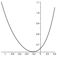
Figure 4. $Y(z)$ has singularities at $z_{r}\doteq 0.3720$ and $z^{\prime}\doteq-1.0079$, where $e^{(1+z)^{2}}(2/3e-\int_{1}^{1+z}e^{-u^{2}}du)=1$.

3.6.2. $N^{v}$ for ${\tt A}_{f}$

In the case of ${\tt A}_{f}$ we have by (3.9) that

$$Y(z)=\frac{1-z}{1-2z(1+z)}.$$

Therefore

$${\bf E}[T_{f}(\pi)^{2}]=[z^{n}]Y(z)\sim z_{f}^{-n}/2$$

where $z_{f}\doteq 0.366$ is the smallest singularity of $Y$, and so

$$N^{v}_{f}\sim\frac{5}{2\varphi^{2}}(z_{f}\varphi^{2})^{-n}.$$

3.6.3. $N^{v}$ for ${\tt A}_{g}$

First, we derive the generating function $X(z,t)$ for the sequence $x_{n}=F_{n,1}{\bf E}_{u}[T(\pi)^{t}]$. The argument is similar to the proof of (3.9) given in Lemma A.1, except that in this case we have $x_{0}=x_{1}=1$, $x_{2}=2^{t+1}$ and for $n\geq 3$,

$$x_{n}=3^{t}(2x_{n-2}+x_{n-3}).$$

Hence

$$X(z,t)=\frac{1+z+2z^{2}(2^{t}-3^{t})}{1-3^{t}z^{2}(2+z)}.$$

Therefore, setting $t=1$,

$$Y(z)=\frac{1+z(1-2z)}{1-3z^{2}(2+z)},$$

and so

$${\bf E}[T_{g}(\pi)^{2}]=[z^{n}]Y(z)\sim\frac{1}{69}(8+17z_{3}+9z_{3}^{2})z_{3}^{-(n+1)}$$

where $z_{3}\doteq 0.3747$ is the smallest singularity of $Y$. Hence

$$N^{v}_{g}\sim\frac{5}{69}(8+17z_{3}+9z_{3}^{2})(z_{3}\varphi^{2})^{-(n+1)}.$$

3.7. Comparison of algorithms

The table appearing below compares the performance of the algorithms studied in this section. The numbers $N^{*}$ are based on $e^{L+\sigma}$ in (2.2). Note that the $e^{L+t}$ bounds of Theorem 2.1 are accurate if ${\bf P}(|\log Y-L|\geq t/2)$ is small. Here ${\bf E}\log Y=L$. More quantitative bounds follow by the one-sided Chebyshev inequalities

$${\bf P}(\log Y-L\geq a\sigma)\leq 1/(1+a^{2}),\quad{\bf P}(\log Y\leq L-a\sigma)\leq 1/(1+a^{2}).$$

Since we have proven normal approximation, we may replace $1/(1+a^{2})$ with $\exp(-a^{2}/2)/(a\sqrt{2\pi})$. We have been content to use $e^{L+\sigma}$ in our numerical examples since simulations show that this is a good indication of the sample size needed.

On the other hand, the numbers $N^{v}$ are based on standard relative variance considerations (2.1). For small values of $n$, these are roughly comparable to the Kullback–Leibler numbers $N^{*}$; however, larger values of $n$ suggest that smaller sample sizes than those given by $N^{v}$ are adequate.

Table 2. Comparison of algorithms ${\tt A}_{r}$, ${\tt A}_{f}$ and ${\tt A}_{g}$ which match in random, fixed and greedy orders. The values $N^{*}$ and $N^{v}$ are the estimates for required sample size given by the Kullback–Leibler (2.2) and relative variance (2.1) criteria.

$n$	200	300	500	1000
$N^{*}_{r}$	$194$	$1211$	$38257$	$1.25\times 10^{8}$
$N^{v}_{r}$	$121$	$1702$	$3.37\times 10^{5}$	$1.86\times 10^{11}$
$N^{*}_{f}$	$1520$	$22479$	$3.75\times 10^{6}$	$6.72\times 10^{11}$
$N^{v}_{f}$	$4884$	$3.50\times 10^{5}$	$1.79\times 10^{9}$	$3.34\times 10^{18}$
$N^{*}_{g}$	$75$	$321$	$4889$	$2.79\times 10^{6}$
$N^{v}_{g}$	$54$	$368$	$17102$	$2.54\times 10^{8}$
$n^{7}$	$1.28\times 10^{16}$	$2.19\times 10^{17}$	$7.82\times 10^{18}$	$1\times 10^{21}$
$F_{n,1}$	$4.54\times 10^{41}$	$3.60\times 10^{62}$	$2.26\times 10^{104}$	$7.04\times 10^{208}$

4. 2-Fibonacci matchings ${\mathcal{F}}_{n,2}$

Next, we consider the class of 2-Fibonacci matchings

$${\mathcal{F}}_{n,2}=\{\pi\in S_{n}:-1\leq\pi(i)-i\leq 2\}.$$

In [11] $t$-Fibonacci matchings ${\mathcal{F}}_{n,t}$ are analyzed in general, however only for fixed order algorithms. Specifically, the mean and variance of $\log T(\pi)$ is computed for algorithm ${\tt A}_{f,2}$ which matches in fixed order $1,2,\ldots,n$. For simplicity, we restrict ourselves to the case $t=2$, although our methods extend to the general case. The cases $t>2$ present no additional challenges, apart from more complicated formulas. The case $t=2$, on the other hand, is more involved than $t=1$, since unlike the case of Fibonacci matchings, after a single $\pi(i)$ is determined by an algorithm, the problem of determining $\pi$ does not necessarily split independently. Note that, given that $\pi(i)\in\{i,i+1,i+2\}$ for some $1<i<n$, the values of $\pi$ on $[i-1]$ and $[n]-[i]$ are independent; but if $\pi(i)=i-1$, this is no longer the case since $\pi(i-1)=i+1$ is possible in a 2-Fibonacci matching.

Figure 5. Perfect matchings in this graph correspond to $2$-Fibonacci permutations in ${\mathcal{F}}_{5,2}$.

We consider sampling using algorithms ${\tt A}_{f,2}$, ${\tt A}_{r,2}$ and ${\tt A}_{g,2}$, which are analogues of ${\tt A}_{f}$, ${\tt A}_{r}$ and ${\tt A}_{g}$ studied in the previous section. Since the calculations become quite lengthy, we will highlight the main differences with the Fibonacci case, but only sketch the details.

Algorithm ${\tt A}_{f,2}$ matches in the fixed order $1,2,\ldots,n$. This case is no more involved than that of ${\tt A}_{f}$ for Fibonacci matchings in any essential way, since this algorithm only ever assigns some $\pi(i)=i-1$ when such a matching is forced due to previous matchings.

On the other hand, some care is required to define tractable analogues ${\tt A}_{r,2}$ and ${\tt A}_{g,2}$. Algorithm ${\tt A}_{r,2}$ matches in a random order, however when an index $i$ is selected, not only is $\pi(i)$ determined, but also the full cycle in $\pi$ containing $i$. In this way ${\tt A}_{r,2}$ matches indices in a small (of minimal size) neighborhood of $i$ so that the further construction of $\pi$ splits into independent parts. More specifically, in the first step of ${\tt A}_{r,2}$ a uniformly random $i\in[n]$ is selected. If $2<i<n-1$, there are six possibilities (see Figure 6) for the cycle in $\pi$ containing $i$, namely

• $\pi(i-2,i-1,i)=i,i-2,i-1$

• $\pi(i-1,i)=i,i-1$

• $\pi(i-1,i,i+1)=i+1,i-1,i$

• $\pi(i)=i$

• $\pi(i,i+1)=i+1,i$

• $\pi(i,i+1,i+2)=i+2,i,i+1$.

If $i\in\{1,2,n-1,n\}$ then only a subset of these are possible. Algorithm ${\tt A}_{r,2}$ selects one of these possibilities at random. The algorithm continues in this way until a 2-Fibonacci permuation $\pi$ is constructed. We note that this algorithm is a natural extension of the Fibonacci case $t=1$ case, since in that case choosing whether $\pi(i)$ is equal to $i-1$, $i$ or $i+1$ is equivalent to selecting the cycle containing $i$.

Figure 6. If index $i$ is selected in some step of algorithm ${\tt A}_{r,2}$, one of the above configurations (or one amongst the remaining allowable options) is selected uniformly at random for $\pi$ near $i$. Note that determining $\pi$ “above and below” this configuration splits independently, since there are no $\pi(j)<j-1$ in a 2-Fibonacci matching.

Finally, we consider the greedy algorithm ${\tt A}_{g,2}$ which in each step, starting with index 3, selects the minimal unmatched index $i$ amongst those with the maximal number of remaining allowable choices for the cycle containing $i$. Similarly as the ${\tt A}_{r,2}$ case, indices are matched in a neighborhood of $i$ by selecting a uniformly random cycle structure for unmatched indices $j\leq i$, and we continue in this way until $\pi$ is constructed.

By the main results of this section, Theorems 4.2, 4.1 and 4.3, and Theorem 2.1 we obtain estimates for the required sample size $N^{*}$ listed in the table below. The greedy algorithm ${\tt A}_{g,2}$, for instance, outperforms $n^{7}$ until about $n=1549$.

Approximate values of $F_{n,2}$ are obtained as follows. By considering whether $\pi(1)$ is equal to 1, 2 or 3, it follows that $F_{n,2}=F_{n-1,2}+F_{n-2,2}+F_{n-3,2}$ for $n\geq 3$. Therefore

(4.1) $$F_{n,2}\sim c_{2}\varphi_{2}^{n+1}$$

where $\varphi_{2}\doteq 1.8393$ satisfies $\varphi_{2}^{3}=\varphi_{2}^{2}+\varphi_{2}+1$ and

$$c_{2}=\frac{1}{22}(3+\frac{7}{\varphi_{2}}+\frac{2}{\varphi_{2}^{2}})\doteq 0.3363.$$

Table 3. Comparison of algorithms ${\tt A}_{r,2}$, ${\tt A}_{f,2}$ and ${\tt A}_{g,2}$ which match in random, fixed and greedy orders. The values $N^{*}$ are the estimates for required sample size given by the Kullback–Leibler (2.2) criterion.

$n$	200	300	500	1000
$N^{*}_{r,2}$	$1.48\times 10^{5}$	$1.49\times 10^{7}$	$1.04\times 10^{11}$	$1.64\times 10^{20}$
$N^{*}_{f,2}$	$5.52\times 10^{8}$	$2.16\times 10^{12}$	$1.95\times 10^{19}$	$1.26\times 10^{36}$
$N^{*}_{g,2}$	$9057$	$2.81\times 10^{5}$	$2.00\times 10^{8}$	$1.27\times 10^{15}$
$n^{7}$	$1.28\times 10^{16}$	$2.19\times 10^{17}$	$7.82\times 10^{18}$	$1\times 10^{21}$
$F_{n,2}$	$5.26\times 10^{52}$	$1.54\times 10^{79}$	$1.31\times 10^{132}$	$2.76\times 10^{264}$

4.1. Random order algorithm ${\tt A}_{r,2}$

We begin with the random order algorithm ${\tt A}_{r,2}$, since it is the most involved of the three. Our discussion of ${\tt A}_{f,2}$ and ${\tt A}_{g,2}$ will be less detailed.

Recall that ${\tt A}_{r,2}$ selects a random index $i$ and then selects a cycle containing $i$ randomly from amongst the allowable options. The algorithm continues in this way until a 2-Fibonacci permutation $\pi$ is obtained.

Theorem 4.1.

Let $P_{r,2}(\pi)$ be the probability of $\pi$ under the random order algorithm ${\tt A}_{r,2}$, where $\pi$ is uniformly random with respect to $u=1/F_{n,2}$ on 2-Fibonacci permutations $\pi\in{\mathcal{F}}_{n,2}$. Put $T_{r,2}(\pi)=P_{r,2}(\pi)^{-1}$. As $n\to\infty$,

$$\frac{\log T_{r,2}(\pi)-\mu_{r,2}n}{\sigma_{r,2}\sqrt{n}}\xrightarrow{d}N(0,1)$$

where $\mu_{r,2}\doteq 0.6465$ and $\sigma^{2}_{r,2}\doteq 0.0799$.

Although it is possible by our arguments to obtain closed form expressions (involving the implicitly defined quantity $\varphi_{2}$ in (4.1)) for the quantities $\mu_{r,2}$ and $\sigma^{2}_{r,2}$, we omit these as they are quite complex.

Proof.

The proof is similar to that of Lemma 3.3. We define $x_{n}$ analogously (replacing $F_{n,1}$ and $T_{r}$ with $F_{n,2}$ and $T_{r,2}$). Then we have that $x_{0}=x_{1}=1$, $x_{2}=2^{t+1}$, $x_{3}=(4/3)[3^{t}(1+2^{t})+4^{t}]$, and for $n\geq 4$,

$$nx_{n}=2(3^{t}-6^{t})(x_{n-1}+x_{n-2}+x_{n-3})+2(5^{t}-6^{t})(2x_{n-2}+2x_{n-3}+x_{n-4})\\ +6^{t}(\sum_{i=0}^{n-1}x_{i}x_{n-i-1}+2\sum_{i=0}^{n-2}x_{i}x_{n-i-2}+3\sum_{i=0}^{n-3}x_{i}x_{n-i-3}).$$

Therefore, along the same lines as (3.4), we find that

$$\frac{\partial}{\partial z}X-1-2^{t+2}z-4[3^{t}(1+2^{t})+4^{t}]z^{2}\\ =2(3^{t}-6^{t})[(1+z+z^{2})X-(1+2z+2(1+2^{t})z^{2})]\\ +2(5^{t}-6^{t})[z(2+2z+z^{2})X-2z(1+2z)]\\ +6^{t}[(1+2z+3z^{2})X^{2}-(1+4z+8(1+2^{t-1})z^{2})]$$

where $X(z,t)$ is the generating function for the sequence of $x_{n}$. Using the asymptotics (4.1) for $F_{n,2}$ and the above equation in place of (3.4), it follows by the the proof of Lemma 3.3 that

$${\bf E}_{u}\log T_{r,2}(\pi)=\mu_{r,2}n+O(1),\quad\mathrm{Var}_{u}\log T_{r,2}(\pi)=\sigma^{2}_{r,2}n+O(1).$$

Indeed, the same strategy of proof works essentially line-for-line, however with more complicated expressions. We omit the details.

To conclude, put $Y_{n}=\log T_{r,2}(\pi)$ and $F_{n,2}=0$ for $n<0$. Note

$$Y_{n}\overset{d}{=}Y^{(1)}_{I_{1}^{(n)}}+Y^{(2)}_{I_{2}^{(n)}}+b_{n},$$

where, for $i\in[n]$,

$${\bf P}((I_{1}^{(n)},I_{2}^{(n)})=(i_{1},i_{2}))\\ =\frac{1}{nF_{n,2}}\begin{cases}F_{i-3,2}F_{n-i,2}&(i_{1},i_{2})=(i-3,n-i)\\ F_{i-2,2}F_{n-i,2}&(i_{1},i_{2})=(i-2,n-i)\\ F_{i-2,2}F_{n-i-1,2}&(i_{1},i_{2})=(i-2,n-i-1)\\ F_{i-1,2}F_{n-i,2}&(i_{1},i_{2})=(i-1,n-i)\\ F_{i-1,2}F_{n-i-1,2}&(i_{1},i_{2})=(i-1,n-i-1)\\ F_{i-1,2}F_{n-i-2,2}&(i_{1},i_{2})=(i-1,n-i-2)\end{cases}$$

and $b_{n}=O(1)$ is equal to $\log 3$, $\log 5$ or $\log 6$ if $i\in\{1,n\}$, $i\in\{2,n-1\}$ or $3\leq i\leq n-2$. Since $I_{1}^{(n)}\overset{d}{=}U_{n}+O(1)$ and $I_{2}^{(n)}\overset{d}{=}n-U_{n}+O(1)$ for $U_{n}$ uniform on $[n]$, the theorem follows by Lemma 3.1. ∎

4.2. Fixed order algorithm ${\tt A}_{f,2}$

Next, we turn to the simpler case of ${\tt A}_{f,2}$ which samples from ${\mathcal{F}}_{n,2}$ by matching indices in $[n]$ in the fixed order $1,2,\ldots,n$, in each step setting $\pi(i)$ equal to one of the remaining allowable options uniformly at random. Note that if previously we have set $\pi(i-2)=i$ or $\pi(i-1)\in\{i,i+1\}$, then $\pi(i)=i-1$ is forced. Otherwise, we set $\pi(i)$ to $i$, $i+1$ or $i+2$ uniformly at random.

Theorem 4.2.

Let $P_{f,2}(\pi)$ be the probability of $\pi$ under the fixed order algorithm ${\tt A}_{f,2}$, where $\pi$ is uniformly random with respect to $u=1/F_{n,2}$ on 2-Fibonacci permutations $\pi\in{\mathcal{F}}_{n,2}$. Put $T_{f,2}(\pi)=P_{f,2}(\pi)^{-1}$. As $n\to\infty$,

$$\frac{\log T_{f,2}(\pi)-\mu_{f,2}n}{\sigma_{f,2}\sqrt{n}}\xrightarrow{d}N(0,1)$$

where $\mu_{f,2}\doteq 0.6794$ and $\sigma^{2}_{f,2}\doteq 0.1592$.

Proof.

The argument is similar to the proof of Theorem 3.4 for ${\tt A}_{f}$. (Alternatively, the central limit theorem for renewal processes can be used, see the proof for ${\tt A}_{g,2}$ below.) In this case, we obtain the generating function

$$X(z,t)=\frac{1+(1-3^{t})z+2(2^{t}-3^{t})z^{2}}{1-3^{t}z(1+z+z^{2})}$$

for the sequence of $x_{n}=F_{n,2}{\bf E}_{u}[T_{f,2}(\pi)^{t}]$. From this, it follows (arguing as in the proof Section A.1) that

$${\bf E}_{u}\log T_{f,2}(\pi)=\mu_{f,2}n+O(1),\quad\mathrm{Var}_{u}\log T_{f,2}(\pi)=\sigma^{2}_{f,2}n+O(1).$$

We omit the details. Hence, as in the proof of Theorem 3.4, the result follows by Lemma 3.1 by considering a modified algorithm ${\tt A}_{f,2}^{\varepsilon}$. ∎

4.3. Greedy algorithm ${\tt A}_{g,2}$

As discussed above, algorithm ${\tt A}_{g,2}$ maximizes the number of steps with 6 choices for the cycle containing $i$. For $n\leq 4$, for simplicity, suppose that ${\tt A}_{g,2}$ selects a uniformly random $\pi\in{\mathcal{F}}_{n,2}$. For $n\geq 5$, starting with index $3$, the smallest unmatched index is selected with the maximal number of choices for the cycle containing $i$. Then a uniformly random cycle structure is chosen for unmatched indices $j\leq i$, and the algorithm continues in this way until $\pi$ is constructed. Note that, for $i\leq n-2$ there are 9 such cycle structures (see Figure 6), since if $\pi(i)\geq i$ then there are 2 choices for the cycle containing $i-1$, either $\pi(i-2,i-1)=i-2,i-1$ or $\pi(i-2,i-1)=i-1,i-2$.

Theorem 4.3.

Let $P_{g,2}(\pi)$ be the probability of $\pi$ under the algorithm ${\tt A}_{g,2}$, where $\pi$ is uniformly random with respect to $u=1/F_{n,2}$ on 2-Fibonacci permutations $\pi\in{\mathcal{F}}_{n,2}$. Put $T_{g,2}(\pi)=P_{g,2}(\pi)^{-1}$. As $n\to\infty$,

$$\frac{\log T_{g,2}(\pi)-\mu_{g,2}n}{\sigma_{g,2}\sqrt{n}}\xrightarrow{d}N(0,1)$$

where $\mu_{g,2}\doteq 0.6365$ and $\sigma^{2}_{g,2}\doteq 0.0514$.

Proof.

This result follows in a similar way as Theorem 3.5, where in this case we compare $\log T_{g,2}(\pi)$ with $N_{n}\log 9$, where $(N_{t},t\geq 0)$ is the renewal process whose inter-arrival times $X_{i}$ are equal to 3, 4 and 5 with probabilities $4/\varphi_{2}^{3}$, $3/\varphi_{2}^{4}$ and $2/\varphi_{2}^{5}$. Since

$$\frac{1}{{\bf E}(X_{1})}\doteq 0.2897,\quad\frac{\mathrm{Var}(X_{1})}{{\bf E}(X_{1})^{3}}\doteq 0.0106,$$

the result follows by the central limit theorem for renewal processes. ∎

4.4. Almost perfect variants

As in Section 3.5 we can, for instance, modify ${\tt A}_{f,2}$ to obtain an “almost perfect” version ${\tt A}_{f,2}^{*}$ (such that $\mathrm{Var}_{u}\log(T_{f,2}^{*}(\pi)/F_{n,2})=O(1)$ under $u=1/F_{n,2}$) by instead setting $\pi(i)$ equal to $i$, $i+1$ and $i+2$ with probabilities $1/\varphi_{2}$, $1/\varphi_{2}^{2}$ and $1/\varphi_{2}^{3}$ (unless $\pi(i)=i-1$ is forced), corresponding to the asymptotic proportions of $\pi$ with $\pi(1)$ equal to 1, 2 and 3. Presumably this reasoning generalizes to all other cases $t\geq 3$.

5. Distance-2 matchings ${\mathcal{D}}_{n,2}$

Finally, we briefly discuss the case of distance-2 matchings

$${\mathcal{D}}_{n,2}=\{\pi\in S_{n}:|\pi(i)-i|\leq 2\}.$$

This class is significantly more complex than the previous cases ${\mathcal{F}}_{n,t}$, as matchings in ${\mathcal{D}}_{n,2}$ can have cycles of all sizes. For instance, such a permutation can even be unicyclic (e.g., $\pi(12345)=24153\in{\mathcal{D}}_{5,2}$). As a result, it seems quite involved to obtain the precise asymptotics for the mean and variance of $\log T(\pi)$ under a random order algorithm ${\tt B}_{r,2}$ (which like ${\tt A}_{r,2}$ selects a random vertex $i$ and then matches around $i$ until the problem of determining $\pi$ splits into independent problems), so we do not pursue this here. However, assuming that $\log T(\pi)$ has asymptotically linear mean and variance, Lemma 3.1 would readily yield a central limit theorem.

In this section, we restrict ourselves to algorithm ${\tt B}_{f,2}$ which matches in the fixed order $1,2,\ldots,n$. We also indicate how to obtain an “almost perfect” version ${\tt B}_{f,2}^{*}$ in Section 5.1.1 below.

Distance-2 matchings are studied in Plouffe’s thesis [31], where in particular the generating function for $D_{n,2}=|{\mathcal{D}}_{n,2}|$ is derived. For completeness, we include the following lemma, which gives the asymptotics of $D_{n,2}$ and the related number $D_{n,2}^{\prime}$ of $\pi\in{\mathcal{D}}_{n,2}$ with $\pi(1)=2$. See Section A.2 for a proof.

Figure 7. Perfect matchings in this graph correspond to distance-2 permutations in ${\mathcal{D}}_{5,2}$.

Lemma 5.1.

For $n\geq 4$,

$$D_{n+1,2}=2D_{n,2}+2D_{n-2,2}-D_{n-4,2}$$

and

$$2D_{n+2,2}^{\prime}=D_{n+1,2}+D_{n,2}+D_{n-1,2}-D_{n-2,2}-D_{n-3,2}.$$

By Lemma 5.1, we find that

(5.1) $$D_{n,2}\sim d_{2}\gamma_{2}^{n+1},\quad D^{\prime}_{n,2}/D_{n,2}\sim\gamma_{2}^{\prime}$$

where $\gamma_{2}\doteq 2.3335$ satisfies $\gamma_{2}^{5}=2\gamma_{2}^{4}+2\gamma_{2}^{2}-1$,

$$d_{2}=\frac{4652\gamma_{2}^{4}+10711\gamma_{2}^{3}+3737\gamma_{2}^{2}-3424\gamma_{2}-2388}{49163\gamma_{2}^{4}}\doteq 0.1948,$$

and

$$\gamma_{2}^{\prime}=(\gamma_{2}^{4}+\gamma_{2}^{3}+\gamma_{2}^{2}-\gamma_{2}-1)/2\gamma_{2}^{5}\doteq 0.3213.$$

Note that, probabilistically, (5.1) says that the chance that a random $\pi\in{\mathcal{D}}_{n,2}$ has $\pi(1)=2$ is approximately $0.32$.

5.1. Fixed order algorithm ${\tt B}_{f,2}$

We consider the algorithm ${\tt B}_{f,2}$ which samples a distance-2 permutation by matching the indices $[n]$ in the fixed order $1,2,\ldots,n$, in each step matching $i$ with a uniformly random index (amongst the remaining allowable options).

In establishing the following central limit theorem for $\log T_{f,2}(\pi)$, our arguments resemble those for Theorems 3.4 and 4.2 (for ${\tt A}_{f}$ and ${\tt A}_{f,2}$), but are significantly complicated by the potential for long cycles in a distance-2 permutation. We sketch the main ideas.

Theorem 5.2.

Let $P_{f,2}(\pi)$ be the probability of $\pi$ under the fixed order algorithm ${\tt B}_{f,2}$, where $\pi$ is uniformly random with respect to $u=1/D_{n,2}$ on distance-2 permutations $\pi\in{\mathcal{D}}_{n,2}$. Put $T_{f,2}(\pi)=P_{f,2}(\pi)^{-1}$. As $n\to\infty$,

$$\frac{\log T_{f,2}(\pi)-\mu_{f,2}n}{\sigma_{f,2}\sqrt{n}}\xrightarrow{d}N(0,1)$$

where $\mu_{f,2}\doteq 0.9053$ and $\sigma_{f,2}^{2}\doteq 0.1147$.

Combining this result with Theorem 2.1, we obtain the following estimates. Algorithm ${\tt B}_{f,2}$ outperforms $n^{7}$ until about $n=617$.

Table 4. Estimates for required sample $N^{*}_{f,2}$ size given by the Kullback–Leibler (2.2) criterion for the fixed order algorithm ${\tt B}_{f,2}$ on distance-2 matchings ${\mathcal{D}}_{n,2}$.

$n$	200	300	400	500
$N^{*}_{f,2}$	$2.85\times 10^{7}$	$2.74\times 10^{10}$	$2.23\times 10^{13}$	$1.63\times 10^{16}$
$n^{7}$	$1.28\times 10^{16}$	$2.19\times 10^{17}$	$1.64\times 10^{18}$	$7.81\times 10^{18}$
$D_{n,2}$	$1.82\times 10^{73}$	$1.15\times 10^{110}$	$7.26\times 10^{146}$	$4.59\times 10^{183}$

Proof.

The mean and variance of $\log T_{f,2}(\pi)$ are derived in [11] (by other methods), but for completeness, we present a concise derivation of these. As in the proofs in Section 3, put $x_{n}=D_{n,2}{\mathbb{E}}[T_{f,2}(\pi)^{t}]$ and $X(z,t)=\sum_{n=0}^{\infty}x_{n}z^{n}$. Recall that $D^{\prime}_{n,2}$ is the number of $\pi\in{\mathcal{D}}_{n,2}$ with $\pi(1)=2$. Similarly, let $D^{\prime\prime}_{n,2}$ be the number of $\pi\in{\mathcal{D}}_{n,2}$ with $\pi(1)=3$. Define $x_{n}^{\prime},X^{\prime}$ and $x_{n}^{\prime\prime},X^{\prime\prime}$ as for $x_{n},X$.

Observe that, for $n\geq 3$,

$$x_{n}=3^{t}(x_{n-1}+x^{\prime}_{n}+x^{\prime\prime}_{n})$$

since in the first step of ${\tt B}_{f,2}$, we set $\pi(1)$ equal to one of $1,2,3$ uniformly at random. Likewise, for $n\geq 4$, it is easy to see that

$$x^{\prime}_{n}=3^{t}(x_{n-2}+x_{n-3}+x^{\prime}_{n-2}),\quad x^{\prime\prime}_{n}=3^{t}(x^{\prime}_{n-1}+x_{n-3}+x_{n-4}).$$

Hence

$$X-1-z-2^{t+1}z^{2}=3^{t}[z(X-1-z)+(X^{\prime}-z^{2})+X^{\prime\prime}]$$

$$X^{\prime}-z^{2}-2^{t+1}z^{3}=3^{t}[z^{2}(X-1-z)+z^{3}(X-1)+z^{2}X^{\prime}]$$

$$X^{\prime\prime}-2^{t+1}z^{3}=3^{t}[z(X^{\prime}-z^{2})+z^{3}(X-1)+z^{4}X].$$

Solving, we obtain $X(z,t)=U(z,t)/V(z,t)$, where

$$U(z,t)=1-(3^{t}-1)z+[2^{t+1}-(2+3^{t})3^{t}]z^{2}\\ +3^{t}[2^{t+2}-1-(2+3^{t})3^{t}]z^{3}+2(2^{t}-3^{t})3^{t}(3^{t}-1)z^{4}-2(2^{t}-3^{t})3^{2t}z^{5}$$

and

$$V(z,t)=1-3^{t}z-3^{t}(1+3^{t})z^{2}-3^{2t}(1+3^{t})(1+z)z^{3}+3^{3t}(1+z)z^{5}.$$

Using this generating function and the asymtotics (5.1), precise asymptotics for the mean and variance of $\log T_{f,2}(\pi)$ can be obtained, arguing as in the proof of Lemma 3.3. We report only the numerical approximations

(5.2) $${\bf E}_{u}\log T_{f,2}(\pi)=0.9053n+O(1),\quad\mathrm{Var}_{u}\log T_{f,2}(\pi)=0.1147n+O(1).$$

Next, we apply Lemma 3.1 to obtain a central limit theorem for $\log T_{f,2}(\pi)$. As in the proofs of Theorems 3.4 and 4.2, we consider a modified algorithm ${\tt B}_{f,2}^{\varepsilon}$ and instead prove a central limit theorem for $\log T^{\varepsilon}_{f,2}(\pi)$. Moreover, as in these proofs, we consider the matching of $k_{n}=\lfloor n/2\rfloor$ and try to split the problem of determining $\pi$ into two independent problems “above and below” $k_{n}$. However, due to the potential for long cycles in a $\pi\in{\mathcal{D}}_{n,2}$, the arguments are slightly more involved.

We call a set of consecutive indices $I\subset[n]$ a block in $\pi$ if all indices in $I$ are matched with indices in $I$. We view a permutation $\pi\in{\mathcal{D}}_{n,2}$ as a sequence of blocks, beginning with the block containing index 1. As noted above, there are unicyclic $\pi\in{\mathcal{D}}_{n,2}$, and so possibly $[n]$ is the only block in $\pi$. However, for $n>3$, there are only two ways in which this can occur (see Figure 8):

• $\pi(1)=2$, $\pi(2)=4$ (so necessarily $\pi(3)=1$); and then $\pi(4)=6$ (so $\pi(5)=3$); and then $\pi(6)=8$ (so $\pi(7)=5$), etc. until finally some $\pi(2i)=2i-1$.

• $\pi(1)=3$, $\pi(2)=1$; and then the above pattern is repeated (but offset by one index) starting with $\pi(3)=5$ (so $\pi(4)=2$), etc.

Figure 8. Block-avoiding configurations in distance-2 matchings.

To complete the proof, let $K_{n}=\{x_{n},\ldots,y_{n}\}$ be the block containing $k_{n}$ in a $\pi\sim u$. As noted already, $K_{n}$ can be large in general, and even possibly $K_{n}=[n]$. The key to applying Lemma 3.1, however, is to note that since $\pi\sim u$, $K_{n}$ is very unlikely to be large. Indeed, since for $n>3$ there are only two block-avoiding patterns, it is easy to see that

(5.3) $${\bf P}_{u}(|K_{n}|=\ell)\leq O(\ell\gamma_{2}^{-\ell})$$

where $\gamma_{2}$ is as in (5.1). Thus, setting $Y_{n}=\log T_{f,2}^{\varepsilon}(\pi)$, we have

$$Y_{n}\overset{d}{=}Y^{(1)}_{x_{n}-1}+Y^{(2)}_{n-y_{n}}+b_{n},$$

where $b_{n}$ is the $\log$ of the probability that, given all indices in $[x_{n}-1]$ are matched correctly, ${\tt B}^{\varepsilon}_{f,2}$ correctly matches those in $K_{n}$. By (5.3) the conditions of Lemma 3.1 are clearly satsified, giving the result. ∎

5.1.1. Almost perfect algorithm ${\tt B}_{f,2}^{*}$

Finally, we briefly explain how to modify algorithm ${\tt B}_{f,2}$ to obtain an “almost perfect” version ${\tt B}_{f,2}^{*}$. It is easiest to describe such an algorithm which in some steps determines the matching of more than one index. As in ${\tt B}_{f,2}$, indices are matched in order $1,2,\ldots,n$. If $i>n-4$, then we set $\pi(i)$ equal to one of the permissible options uniformly at random. If, on the other hand, $i\leq n-4$, then we consider two cases. Recall $\gamma_{2}$ and $\gamma_{2}^{\prime}$ in (5.1).

1. If all indices in $[i]$ have been matched with indices in $[i]$, then algorithm ${\tt B}_{f,2}^{*}$ sets

   • $\pi(i+1)=i+1$ with probability $1/\gamma_{2}$

   • $\pi(i+1)=i+2$ with probability $\gamma_{2}^{\prime}$

   • $\pi(i+1,i+2)=i+3,i+1$ with probability $\gamma_{2}^{\prime}/\gamma_{2}$

   • $\pi(i+1,i+2,i+3)=i+3,i+2,i+3$ with probability $1/\gamma_{2}^{3}$

   • $\pi(i+1,i+2,i+3,i+4)=i+3,i+4,i+1,i+2$ with probability $1/\gamma_{2}^{4}$.

2. On the other hand, if all indices in $[i]$ have been matched with indices in $[i+1]-\{i\}$, then algorithm ${\tt B}_{f,2}^{*}$ sets

   • $\pi(i+1)=i$ with probability $1/\gamma_{2}^{\prime}\gamma_{2}^{2}$

   • $\pi(i+1,i+2)=i+2,i$ with probability $1/\gamma_{2}^{\prime}\gamma_{2}^{3}$

   • $\pi(i+1,i+2)=i+3,i$ with probability $1/\gamma_{2}^{2}$.

The reason for the choices in (1) is that $1/\gamma_{2}$, $\gamma_{2}^{\prime}$, $\gamma_{2}^{\prime}/\gamma_{2}$, $1/\gamma_{2}^{3}$ and $1/\gamma_{2}^{4}$ are the asymptotic proportions of matchings in ${\mathcal{D}}_{n,2}$ with $\pi(1)=1$, $\pi(1)=2$, $\pi(12)=31$, $\pi(123)=321$ and $\pi(1234)=3412$. The probabilities in (2) are chosen similarly, considering the asymptotic proportions of matchings in ${\mathcal{D}}_{n,2}^{\prime}$ with $\pi(2)=1$, $\pi(23)=31$ and $\pi(23)=41$.

Defining $x_{n},X$ and $x_{n}^{\prime},X^{\prime}$ as in previous proofs, in this case we obtain $x_{0}=x_{1}=1$, $x_{2}=2^{t+1}$, $x_{0}^{\prime}=x_{1}^{\prime}=0$, $x_{2}^{\prime}=1$ and $x_{3}^{\prime}=2^{t+1}$, and for $n\geq 4$,

$$x_{n} =\gamma_{2}^{t}x_{n-1}+(1/\gamma_{2}^{\prime})^{t}x^{\prime}_{n}+(\gamma_{2}/\gamma_{2}^{\prime})^{t}x^{\prime}_{n-1}+\gamma_{2}^{3t}x_{n-3}+\gamma_{2}^{4t}x_{n-4}$$

$$x^{\prime}_{n} =(\gamma_{2}^{\prime}\gamma_{2}^{2})^{t}x_{n-2}+(\gamma_{2}^{\prime}\gamma_{2}^{3})^{t}x_{n-3}+\gamma_{2}^{2t}x^{\prime}_{n-2}.$$

Therefore

$$X-1-z-2^{t+1}z^{2}-2^{t+1}3^{t+1}z^{3}\\ =\gamma_{2}^{t}z(X-1-z-2^{t+1}z^{2})+(1/\gamma_{2}^{\prime})^{t}(X^{\prime}-z^{2}-2^{t+1}z^{3})\\ +(\gamma_{2}/\gamma_{2}^{\prime})^{t}z(X^{\prime}-z^{2})+\gamma_{2}^{3t}z^{3}(X-1)+\gamma_{2}^{4t}z^{4}X$$

and

$$X^{\prime}-z^{2}-2^{t+1}z^{3}=(\gamma_{2}^{\prime}\gamma_{2}^{2})^{t}z^{2}(X-1-z)+(\gamma_{2}^{\prime}\gamma_{2}^{3})^{t}z^{3}(X-1)+\gamma_{2}^{2t}z^{2}X^{\prime}.$$

Hence $X(z,t)=U(z,t)/V(z,t)$, where

$$U(z,t)=1+(1-\gamma_{2}^{t})z\\ +(2^{t+1}-\gamma_{2}^{t}-2\gamma_{2}^{2t})z^{2}+(6^{t+1}-2(2\gamma_{2})^{t}-2\gamma_{2}^{2t}-2\gamma_{2}^{3t})z^{3}\\ +\gamma_{2}^{t}(2(2/\gamma_{2}^{\prime})^{t}+(\gamma_{2}/\gamma_{2}^{\prime})^{t}-2(2\gamma_{2})^{t}-\gamma_{2}^{3t})z^{4}\\ +\gamma_{2}^{2t}(-6^{t+1}+2(2/\gamma_{2}^{\prime})^{t}+2(2\gamma_{2})^{t}+(\gamma_{2}/\gamma_{2}^{\prime})^{t}+\gamma_{2}^{3t})z^{5}$$

and

$$V(z,t)=1-\gamma_{2}^{t}z-2\gamma_{2}^{2t}z^{2}-2\gamma_{2}^{3t}z^{3}-2\gamma_{2}^{4t}z^{4}+\gamma_{2}^{5t}z^{5}+\gamma_{2}^{6t}z^{6}.$$

Using this generating function, it can be shown that

$${\bf E}_{u}\log T(\pi)/n\to\log\gamma_{2},\quad\mathrm{Var}_{u}\log T(\pi)=O(1).$$

Hence, by Theorem 2.1, $N^{*}(n)=O(1)$ samples are sufficient to well approximate ${\mathcal{D}}_{n,2}$ by this algorithm.

Appendix A Supplementary results

A.1. Mean and variance for ${\tt A}_{f}$

In this section we establish (3.10) giving the asymptotics for the mean and variance of $\log T_{f}(\pi)$ under the uniform distribution $u=1/F_{n,1}$.

Lemma A.1.

As $n\to\infty$,

$${\bf E}_{u}\log T_{f}(\pi)\sim\mu_{f}n+\frac{2(1-\sqrt{5})}{5}\log 2$$

and

$$\mathrm{Var}_{u}\log T_{f}(\pi)\sim\sigma^{2}_{f}n+\frac{11\sqrt{5}-27}{25}\log^{2}2,$$

where

$$\mu_{f}=\frac{1}{2}(1+\frac{1}{\sqrt{5}})\log 2,\quad\sigma^{2}_{f}=\frac{1}{5\sqrt{5}}\log^{2}2.$$

Proof.

As in the proof of Lemma 3.3, let $x_{n}=F_{n,1}{\bf E}_{u}[T_{f}(\pi)^{t}]$. Let $X(z,t)$ be the associated generating function, and note that

$${\mathbb{E}}_{u}[(\log T_{f}(\pi))^{k}]=\frac{1}{F_{n,1}}[z^{n}]\frac{\partial^{k}}{\partial t^{k}}X(z,0).$$

Clearly, $x_{0}=x_{1}=1$. For $n\geq 2$, note that ${\bf P}_{u}(\pi(1)=1)=F_{n-1,1}/F_{n,1}$ and ${\bf P}_{u}(\pi(1)=2)=F_{n-2,1}/F_{n,1}$, and in either case ${\tt A}_{f}$ correctly matches $1$ with $\pi(1)$ with probability $1/2$. Therefore, for $n\geq 2$, we have that

$$x_{n}=2^{t}(x_{n-1}+x_{n-2}).$$

Summing over $n\geq 2$, it follows that

$$X-1-z=2^{t}[z(X-1)+z^{2}X]$$

and so, as stated in (3.9),

$$X(z,t)=\frac{1+(1-2^{t})z}{1-2^{t}z(1+z)}.$$

Therefore

$$(1-z-z^{2})^{2}\frac{\partial}{\partial t}X(z,t)=z^{2}(2+z)\log 2$$

and

$$(1-z-z^{2})^{3}\frac{\partial^{2}}{\partial t^{2}}X(z,t)=z^{2}(2+z)(1+z+z^{2})\log^{2}2.$$

Hence the lemma follows, arguing as in the proof of Lemma 3.3, using the asymptotics (3.7) and (3.8). Indeed, let $A_{n}$ and $B_{n}$ denote the right hand sides of (3.7) and (3.8). By the above arguments, we find that

$${\bf E}_{u}\log T_{f}(\pi)\sim[\frac{A_{n-3}}{\varphi^{3}}+2\frac{A_{n-2}}{\varphi^{2}}]\log 2\\ =\mu_{f}n+\frac{2(1-\sqrt{5})}{5}\log 2$$

and

$${\bf E}_{u}[(\log T_{f}(\pi))^{2}]\sim[\frac{B_{n-5}}{\varphi^{5}}+3\frac{B_{n-4}}{\varphi^{4}}+3\frac{B_{n-3}}{\varphi^{3}}+2\frac{B_{n-2}}{\varphi^{2}}]\log^{2}2\\ =(\mu_{f}n)^{2}-\frac{1}{25}[7\sqrt{5}n+3(\sqrt{5}-1)]\log^{2}2.$$

Hence

$$\mathrm{Var}_{u}\log T_{f}(\pi)\sim\sigma_{f}^{2}+\frac{11\sqrt{5}-27}{25}\log^{2}2$$

completing the proof. ∎

A.2. Distance-2 asymptotics

In order to prove Lemma 5.1, we first establish the following observation.

Lemma A.2.

For $n\geq 4$,

$$D_{n,2}=D_{n-1,2}+D^{\prime}_{n,2}+D^{\prime}_{n-1,2}+D_{n-3,2}+D_{n-4,2}$$

and

$$D^{\prime}_{n,2}=D_{n-2,2}+D_{n-3,2}+D^{\prime}_{n-2,2}=\sum_{k=0}^{n-2}D_{k,2}.$$

Proof.

Indeed, to see the first equality, note that there are $D_{n-1,2}$ matchings with $\pi(1)=1$; $D^{\prime}_{n,2}$ with $\pi(1)=2$; $D^{\prime}_{n-1,2}$ with $\pi(1)=3$ and $\pi(2)=1$; $D_{n-3,2}$ with $\pi(1)=3$ and $\pi(2)=2$ (so necessarily $\pi(3)=1$); and $D_{n-4,2}$ with $\pi(1)=3$ and $\pi(2)=4$ (so necessarily $\pi(3)=1$ and $\pi(4)=2$). The second equality is similarly derived. ∎

Using these formulas, we deduce the result.

Proof of Lemma 5.1.

The first equality follows immediately by Lemma A.2, noting that for all $n\geq 4$,

$$D_{n+1,2}-D_{n,2}=D_{n,2}-D_{n-1,2}+D_{n-2,2}-D_{n-4,2}+D^{\prime}_{n+1,2}-D^{\prime}_{n-1,2}$$

and $D^{\prime}_{n+1,2}-D^{\prime}_{n-1,2}=D_{n-1,2}+D_{n-2,2}$.

Then, for the second equality, note that by the first, for all $k\geq 4$, we have

$$D_{k+1,2}-D_{k,2}=D_{k,2}+2D_{k-2,2}-D_{k-4,2}.$$

Summing over $4\leq k\leq n$, we find

$$D_{n+1,2}-D_{4,2}=2\sum_{k=0}^{n}D_{k,2}-(D_{0,2}+D_{1,2}+D_{2,2}+D_{3,2})\\ -2(D_{0,2}+D_{1,2}+D_{n-1,2}+D_{n,2})+(D_{n-3,2}+D_{n-2,2}+D_{n-1,2}+D_{n,2}),$$

and the result follows noting that $D_{0,2}=D_{1,2}=1$, $D_{2,2}=2$, $D_{3,2}=6$ and $D_{4,2}=14$, and recalling that, by Lemma A.2, $D^{\prime}_{n+2,2}=\sum_{k=0}^{n}D_{k,2}$. ∎

References

• [1] R. B. Bapat, Permanents in probability and statistics, Linear Algebra Appl. 127 (1990), 3–25.
• [2] A. D. Barbour, L. Holst, and S. Janson, Poisson approximation, Oxford Studies in Probability, vol. 2, The Clarendon Press, Oxford University Press, New York, 1992, Oxford Science Publications.
• [3] A. Barvinok, Combinatorics and complexity of partition functions, Algorithms and Combinatorics, vol. 30, Springer, Cham, 2016.
• [4] I. Bezáková, D. Štefankovič, V. V. Vazirani, and E. Vigoda, Accelerating simulated annealing for the permanent and combinatorial counting problems, SIAM J. Comput. 37 (2008), no. 5, 1429–1454.
• [5] J. Blitzstein and P. Diaconis, A sequential importance sampling algorithm for generating random graphs with prescribed degrees, Internet Math. 6 (2010), no. 4, 489–522.
• [6] O. Blumberg, Cutoff for the transposition walk on permutations with one-sided restrictions, preprint (2012), available at arXiv:1202.4797.
• [7] by same author, Permutations with interval restrictions, Ph.D. thesis, Stanford University, 2012.
• [8] L. M. Brègman, Certain properties of nonnegative matrices and their permanents, Dokl. Akad. Nauk SSSR 211 (1973), 27–30.
• [9] S. Chatterjee and P. Diaconis, The sample size required in importance sampling, Ann. Appl. Probab. 28 (2018), no. 2, 1099–1135.
• [10] Y. Chen, P. Diaconis, S. P. Holmes, and J. S. Liu, Sequential Monte Carlo methods for statistical analysis of tables, J. Amer. Statist. Assoc. 100 (2005), no. 469, 109–120.
• [11] F. Chung, P. Diaconis, and R. Graham, Permanental generating functions and sequential importance sampling, Adv. in Appl. Math., in press, available online (2019) at https://doi.org/10.1016/j.aam.2019.05.004.
• [12] F. R. K. Chung, P. Diaconis, R. L. Graham, and C. L. Mallows, On the permanents of complements of the direct sum of identity matrices, Adv. in Appl. Math. 2 (1981), no. 2, 121–137.
• [13] P.-T. de Boer, D. P. Kroese, S. Mannor, and R. Y. Rubinstein, A tutorial on the cross-entropy method, Ann. Oper. Res. 134 (2005), 19–67.
• [14] P. Diaconis, Sequential importance sampling for estimating the number of perfect matchings in bipartite graphs: An ongoing conversation with laci, Building Bridges II, Bolyai Society Mathematical Studies, vol. 28, Springer, Berlin, Heidelberg, 2019, pp. 223–233.
• [15] P. Diaconis and R. Graham, The analysis of sequential experiments with feedback to subjects, Ann. Statist. 9 (1981), no. 1, 3–23.
• [16] P. Diaconis, R. Graham, and S. P. Holmes, Statistical problems involving permutations with restricted positions, State of the art in probability and statistics (Leiden, 1999), IMS Lecture Notes Monogr. Ser., vol. 36, Inst. Math. Statist., Beachwood, OH, 2001, pp. 195–222.
• [17] M. Dyer, M. Jerrum, and H. Müller, On the switch Markov chain for perfect matchings, Proceedings of the Twenty-Seventh Annual ACM-SIAM Symposium on Discrete Algorithms, ACM, New York, 2016, pp. 1972–1983.
• [18] B. Efron and V. Petrosian, A simple test of independence for truncated data with applications to red shift surveys, Astrophysical Journal 399 (1992), 345–352.
• [19] P. Flajolet and R. Sedgewick, Analytic combinatorics, Cambridge University Press, Cambridge, 2009.
• [20] H.-K. Hwang and R. Neininger, Phase change of limit laws in the quicksort recurrence under varying toll functions, SIAM J. Comput. 31 (2002), no. 6, 1687–1722.
• [21] M. Jerrum, A. Sinclair, and E. Vigoda, A polynomial-time approximation algorithm for the permanent of a matrix with nonnegative entries, J. ACM 51 (2004), no. 4, 671–697.
• [22] D. Knuth, private communication.
• [23] J. S. Liu, Monte Carlo strategies in scientific computing, Springer Series in Statistics, Springer, New York, 2008.
• [24] L. Lovász and M. D. Plummer, Matching theory, North-Holland Mathematics Studies, vol. 121, North-Holland Publishing Co., Amsterdam; North-Holland Publishing Co., Amsterdam, 1986, Annals of Discrete Mathematics, 29.
• [25] S. Melczer, An invitation to analytic combinatorics: From one to several variables, Springer Texts & Monographs in Symbolic Computation (undergoing editing), 2020.
• [26] P. R. Milgrom and J Roberts, Economics, organization, and management, Prentice Hall, 1992.
• [27] R. Neininger, private communication.
• [28] by same author, Refined Quicksort asymptotics, Random Structures Algorithms 46 (2015), no. 2, 346–361.
• [29] R. Neininger and L. Rüschendorf, A general limit theorem for recursive algorithms and combinatorial structures, Ann. Appl. Probab. 14 (2004), no. 1, 378–418.
• [30] B. Pittel, Normal convergence problem? Two moments and a recurrence may be the clues, Ann. Appl. Probab. 9 (1999), no. 4, 1260–1302.
• [31] S. Plouffe, Approximations de séries génératrices et quelques conjectures, Ph.D. thesis, Université du Québec à Montréal, 1992.
• [32] A. Tsao, Sampling algorithms for intractable counting problems, Ph.D. thesis, Stanford University, 2020.
• [33] L. G. Valiant, The complexity of computing the permanent, Theoret. Comput. Sci. 8 (1979), no. 2, 189–201.