Global dynamics and spatio-temporal patterns of predator-prey systems with density-dependent motion

Abstract: In this paper, we investigate the global boundedness, asymptotic stability and pattern formation of predator-prey systems with density-dependent preytaxis in a two-dimensional bounded domain with Neumann boundary conditions, where the coefficients of motility (diffusion) and mobility (preytaxis) of the predator are correlated through a prey density dependent motility function. We establish the existence of classical solutions with uniform-in time bound and the global stability of the spatially homogeneous prey-only steady states and coexistence steady states under certain conditions on parameters by constructing Lyapunov functionals. With numerical simulations, we further demonstrate that spatially homogeneous time-periodic patterns, stationary spatially inhomogeneous patterns and chaotic spatio-temporal patterns are all possible for the parameters outside the stability regime. We also find from numerical simulations that the temporal dynamics between linearized system and nonlinear systems are quite different, and the prey density-dependent motility function can trigger the pattern formation.

Keywords: Predator-prey system, prey-taxis, boundedness, global stability, Lyapunov functional.

2010 Mathematics Subject Classification: 35A01, 35B40, 35B44, 35K57, 35Q92, 92C17.

1. Introduction

The foraging is the searching for wild food resources by hunting, fishing, consuming or the gathering of plant matter. It plays an important role in an organism’s ability to survive and reproduce. The nonrandom foraging strategies in the predator-prey dynamics, such as the area-restricted search, is often observed to result in populations of predators moving (or flowing) toward regions of higher prey density (see [9, 7, 30, 31]). Such movement is referred to as preytaxis which has important roles in biological control or ecological balance such as regulating prey (pest) population to avoid incipient outbreaks of prey or forming large-scale aggregation for survival (cf. [34, 30, 11]). To understand the dynamics of predator-prey systems with prey-taxis, Karevia and Odell [17] put individual foraging behaviors into a biased random walk model which, upon passage to a continuum limit, leads to the following preytaxis system (see equations (55)-(56) in [17]):

$$\left\{\begin{array}[]{lll}\partial_{t}u=\nabla\cdot(d(v)\nabla u)-\nabla\cdot(u\chi(v)\nabla v)+\mathcal{F}(u,v),\\ \partial_{t}v=D\Delta v+\mathcal{G}(u,v),\end{array}\right.$$ (1.3)

where $u=u(x,t)$ and $v=v(x,t)$ denote the population density of predators and preys at position $x$ and time $t$, respectively, and $D>0$ is a constant denoting the diffusivity of preys. The term $\nabla\cdot(d(v)\nabla u)$ describes the diffusion (motility) of predators with coefficient $d(v)$, and $-\nabla\cdot(u\chi(v)\nabla v)$ accounts for the prey-taxis (mobility) with coefficient $\chi(v)$, where both motility and mobility coefficients are related to individual foraging behaviors. The source terms $\mathcal{F}(u,v)$ and $\mathcal{G}(u,v)$ represent the predator-prey interactions to be discussed below. By fitting the abstract model (1.3) to field experiment data of area-restricted search behavior exhibited by individual ladybugs (predators) and aphids (prey) with appropriate predator-prey interactions (see [17]), Karevia and Odell showed that the area-restricted non-random foraging yield heterogeneous aggregative patterns observed in the field experiment.

In a special case $\chi(v)=-d^{\prime}(v)$, the system (1.3) becomes

$$\left\{\begin{array}[]{lll}\partial_{t}u=\Delta(d(v)u)+\mathcal{F}(u,v),\\ \partial_{t}v=D\Delta v+\mathcal{G}(u,v),\end{array}\right.$$

where the diffusion term $\Delta(d(v)u)$ with $d^{\prime}(v)<0$ has been interpreted as “density-suppressed motility” in [10, 25](see more in [14, 35]), and $d(v)$ is called the motility function. This means that the predator will reduce its motility when encountering the prey, which is a rather reasonable assumption and has very sound applications in the predator-prey systems.

As mentioned in [17], the model (1.3) was tailored to study the non-random foraging behavior (or prey-taxis) not only for ladybugs and aphids, but also for general organisms living in the predator-prey system. Formally the model (1.3) can be regarded as a variant of the Keller-Segel chemotaxis model [18], where $u(x,t)$ denotes the cell density and $v(x,t)$ the chemical concentration. However the prey-taxis model (1.3) has two striking features that the Keller-Segel models have not considered yet. First the model (1.3) characterizes the non-random population dispersal and aggregation (i.e. both diffusion and prey-taxis coefficients depend on the prey density). Second, the source terms in (1.3) have the inter-specific interactions. These two features distinguish the prey-taxis model from the Keller-Segel type chemotaxis models.

Ecological/biological interactions can be defined as either intra-specific or inter-specific. The former occurs between individuals of the same species, while the later between two or more species. There are three types of basic interspecific interactions (see [8, 15, 24]): predator-prey, competition and mutualism, which can be encapsulated in $\mathcal{F}(u,v)$ and $\mathcal{G}(u,v)$ by the following typical form:

$$\mathcal{F}(u,v)=c_{1}uF(v)+h(u),\ \ \mathcal{G}(u,v)=f(v)-c_{2}uF(v)$$ (1.5)

where $h(u)$ and $f(v)$ are functions representing the intra-specific interactions of predators and preys, respectively. Parameters $c_{1},c_{2}\in\mathbb{R}$ denote the coefficients of inter-specific interactions between predators and preys, where $F(v)$ is commonly called the functional response function fulfilling $F(0)=0,\ F^{\prime}(v)>0$. This paper is interested in the predator-prey interaction where $c_{1}>0,c_{2}>0$. The function forms given in (1.5) have represented most of ecologically meaningful examples of predator-prey population interactions used in the literature by assigning appropriate expressions to $h(u)$, $f(v)$ and $F(v)$. Typically the predator kinetics $h(u)$ may include density dependent death $h(u)=-u(\theta+\alpha u),\theta>0,\alpha\geq 0$ , the prey kinetics $f(v)$ could be linear, logistic or Allee effect (bistable) type, and $F(v)$ may be of Lotka-Volterra type [26, 41] or Holling’s type [12]. We refer the readers to the excellent surveys [29, 40] for an exhaustive list of $h(u),f(v)$ and $F(v)$. Hence in this paper we consider the following system

$$\begin{cases}u_{t}=\nabla\cdot(d(v)\nabla u)-\nabla\cdot(u\chi(v)\nabla v)+\gamma uF(v)-\theta u-\alpha u^{2},&x\in\Omega,~{}~{}t>0,\\ v_{t}=D\Delta v-uF(v)+f(v),&x\in\Omega,~{}~{}t>0,\\ \frac{\partial u}{\partial\nu}=\frac{\partial v}{\partial\nu}=0,&x\in\partial\Omega,~{}~{}t>0,\\ u(x,0)=u_{0}(x),v(x,0)=v_{0}(x),&x\in\Omega,\\ \end{cases}$$ (1.6)

where $D,\gamma>0,\theta>0,\alpha\geq 0$ are constants, and $d(v),\chi(v),F(v)$ and $f(v)$ satisfy the following conditions:

• $d(v),\chi(v)\in C^{2}([0,\infty)),d(v)>0,{\color[rgb]{0,0,0}\chi(v)\geq 0}$ and ${\color[rgb]{0,0,0}d^{\prime}(v)\leq 0}$ on $[0,\infty)$.

• $F(v)\in{\color[rgb]{0,0,0}C^{1}([0,\infty))},~{}F(0)=0,~{}F(v)>0~{}\mathrm{in}~{}(0,\infty)~{}\mathrm{and}~{}F^{\prime}(v)>0$.

• $f:[0,\infty)\to\mathbb{R}$ is in $C^{1}$ with $f(0)=0$, and there exist two constants $\mu,K>0$ such that $f(v)\leq\mu v$ for any $v\geq 0$, $f(K)=0$ and $f(v)<0$ for all $v>K$.

We remark that the above assumptions for $F(v)$ and $f(v)$ have covered a large class of interesting and meaningful examples encountered in the literature as mentioned above. Our first result on the global boundedness of solutions of (1.6) is the following.

Theorem 1.1 (Global boundedness).

Assume $(u_{0},v_{0})\in[W^{1,p}(\Omega)]^{2}$ with $p>2$ and $u_{0},v_{0}\geq 0(\not\equiv 0)$. Let $\Omega\subset\mathbb{R}^{2}$ be a bounded domain with smooth boundary and the hypotheses (H1)-(H3) hold. If $\alpha>0$ or $\chi(v)=-d^{\prime}(v)$, then there is a unique classical solution $(u,v)\in[C([0,\infty)\times\bar{\Omega})\cap C^{2,1}((0,\infty)\times\bar{\Omega})]^{2}$ solving the problem (1.6). Moreover there is constant $C>0$ independent of $t$ such that

$$\|u(\cdot,t)\|_{L^{\infty}}+\|v(\cdot,t)\|_{W^{1,\infty}}\leq C,$$

where in particular $0\leq v\leq K_{0}$ with

$$K_{0}:=\max\{\|v_{0}\|_{L^{\infty}},K\}.$$ (1.7)

Next, we will study the large time behavior of solutions. One can easily compute that the system (1.6) has three homogeneous steady states $(u_{s},v_{s})$:

$$(u_{s},v_{s})=\begin{cases}(0,0)\ \mathrm{or}\ (0,K),&\mathrm{if}\ \gamma F(K)\leq\theta{\color[rgb]{0,0,0},}\\ (0,0)\ \mathrm{or}\ (0,K)\ \mathrm{or}\ (u_{*},v_{*}),&\mathrm{if}\ \gamma F(K)>\theta\\ \end{cases}$$

with $u_{*},v_{*}>0$ determined by the following algebraic equations:

$$u_{*}=\frac{f(v_{*})}{F(v_{*})},\ \gamma F(v_{*})=\theta+\alpha u_{*},$$ (1.8)

where $(0,0)$ is the extinction steady state, $(0,K)$ is the prey-only steady state and $(u_{*},v_{*})$ is the coexistence steady state. As in [13], for the global stability, along with the hypotheses (H1)-(H3), we need another condition for the following compound function:

$$\phi(v)=\frac{f(v)}{F(v)}$$

as follows:

(H4) The function $\phi(v)$ is continuously differentiable on $(0,\infty)$, $\phi(0)=\lim\limits_{v\to 0}\phi(v)>0$ and $\phi^{\prime}(v)<0$ for any $v\geq 0$.

Then the global stability results are given as follows:

Theorem 1.2 (Global stability).

Let the hypotheses (H1)-(H4) and assumptions in Theorem 1.1 hold. Then the solution $(u,v)$ obtained in Theorem 1.1 has the following properties:

1. If the parameters $\theta,\gamma,K$ satisfy $\gamma F(K)\leq\theta$ where “$=$” holds iff $\alpha>0$, then

   $$\|u\|_{L^{\infty}}+\|v-K\|_{L^{\infty}}\to 0\ \text{as}\ t\to\infty$$

   exponentially if $\gamma F(K)<\theta$ or algebraically if $\gamma F(K)=\theta,\alpha>0$.

2. If the parameters $\theta,\gamma,K$ satisfy $\gamma F(K)>\theta$ and

   $$D\geq\max\limits_{0\leq v\leq K_{0}}{\color[rgb]{0,0,0}\frac{u_{*}|F(v)|^{2}|\chi(v)|^{2}}{4\gamma F(v_{*})F^{\prime}(v)d(v)}},$$

   then

   $$\|u-u_{*}\|_{L^{\infty}}+\|v-v_{*}\|_{L^{\infty}}\to 0\ \text{as}\ t\to\infty,$$

   where the convergence is exponential if $\alpha>0$.

We remark if $d(v)$ and $\chi(v)$ are constant, the system (1.3) has been studied from various aspects (cf. [2, 6, 23, 24, 37, 46]), and in particular the global existence and stability of solutions have been established in a previous work by the authors in [13]. The results Theorem 1.1 and 1.2 extend the results of [13] to nonconstant $d(v)$ and $\chi(v)$. Moreover the proof of Theorem 1.2 uses a similar idea (method of Lyaunoval functional) as in [13]. Except these analogies, we would like to stress some essential differences between the present paper and [13] below.

• The method used in [13] to prove the global existence of solutions was based on a priori estimate for the energy functional $\int_{\Omega}u\ln udx$ to attain the $L^{2}$-estimate of solutions. However such a priori estimates is attainable only for case where the motility function $d(v)$ is constant. Hence the method of [13] is inapplicable to the model (1.6). In this paper, we estimate $L^{2}$-norm of solutions directly to obtain the global existence of solutions (see section 3). With this new direct $L^{2}$-estimate method, the concavity of $F(v)$ required in [13] is no longer needed. That is we not only use a different method to prove the global boundedness of solutions but also remove the condition $F^{\prime\prime}(v)\leq 0$ imposed in [13].

• If $d(v)$ and $\chi(v)$ are non-constant as considered in this paper, we find that the system (1.6) can generate pattern formation as shown in section 5. This is different from [13] where no pattern formation can be founded for constant $d(v)$ and $\chi(v)$. Our result indicates that the density-dependent motility is a trigger for pattern formation, which is a new finding.

• In the proof of global stability shown in section 4, we need the estimate of $\|\nabla u\|_{L^{4}}$ which can be easily obtained for constant $d(v)$ and $\chi(v)$ but is not clear if $d(v)$ and $\chi(v)$ are not constant. Hence we present a new proof in Lemma 4.2.

In section 5, we shall detail the results of Theorem 1.1 and Theorem 1.2 for specific and often used forms of $F(v)$. In Theorem 1.2 the conditions on parameter values are identified to ensure the global stability of homogeneous steady states. However it is unknown whether non-homogeneous (i.e., non-constant) steady states exists outside the stability regimes found in Theorem 1.2. In the final section 5, we shall use linear stability analysis to find the conditions on parameters for the instability of equilibria of (1.6) and then perform numerical simulations to illustrate that indeed spatially inhomogeneous patterns and time-periodic patterns can be found under certain conditions. We also demonstrate that the nonconstant motility function $d(v)$ plays an important role in generating the pattern formation.

2. Local existence and Preliminaries

In what follows, we shall use $c_{i}$ or $C_{i}(i=1,2,3,\cdots$) to denote a generic constant which may vary in the context. We first state the existence of local-in-time classical solutions of system (1.6) by using the abstract theory of quasilinear parabolic systems in [5].

Lemma 2.1 (Local existence).

Let $\Omega$ be a bounded domain in $\mathbb{R}^{2}$ with smooth boundary and the hypotheses (H1)-(H3) hold. Assume $(u_{0},v_{0})\in[W^{1,p}(\Omega)]^{2}$ with $u_{0},v_{0}\geq 0(\not\equiv 0)$ and $p>2$. Then there exists $T_{max}\in(0,\infty]$ such that the problem (1.6) has a unique classical solution $(u,v)\in[C([0,T_{max})\times\bar{\Omega})\cap C^{2,1}((0,T_{max})\times\bar{\Omega})]^{2}$ satisfying $u,v\geq 0$ for all $t>0$. Moreover, we have

$$either\ \ T_{max}=\infty,\ or\ \ \limsup\limits_{t\nearrow T_{max}}(\|u(\cdot,t)\|_{L^{\infty}}+\|v(\cdot,t)\|_{L^{\infty}})=\infty.$$ (2.1)

Proof.

We shall apply the theory developed by Amann [5] to prove this lemma. With $\omega=(u,v)$, the system (1.6) can be reformulated as

$$\begin{cases}\omega_{t}=\nabla\cdot(\mathbb{A}(\omega)\nabla\omega)+\Phi(\omega),&x\in\Omega,t>0,\\ \frac{\partial\omega}{\partial\nu}=0,&x\in\partial\Omega,t>0,\\ \omega(\cdot,0)=(u_{0},v_{0}),&x\in\Omega,\end{cases}$$

where

$$\mathbb{A}(\omega)=\begin{bmatrix}d(v)&-\chi(v)u\\[2.84526pt] 0&1\end{bmatrix}\ \mathrm{and}\ \ \Phi(\omega)=\begin{bmatrix}\gamma uF(v)-\theta u-\alpha u^{2}\\ f(v)-uF(v)\end{bmatrix}.$$

Since the given initial conditions satisfy $0\leq(u_{0},v_{0})\in[W^{1,p}(\Omega)]^{2}$ with $p>2$ and hence the matrix $\mathbb{A}(\omega)$ is positively definite at $t=0$. Hence the system (1.6) is normally parabolic and the local existence of solutions follows from [4, Theorem 7.3]. That is there exists a $T_{max}>0$ such that the system (1.6) admits a unique solution $(u,v)\in[C([0,T_{max})\times\bar{\Omega})\cap C^{2,1}((0,T_{max})\times\bar{\Omega})]^{2}$.

Next, we will use the maximum principle to prove that $u,v\geq 0$. To this end, we rewrite the first equation of (1.6) as

$$u_{t}=d(v)\Delta u+[d^{\prime}(v)\nabla v-\chi(v)\nabla v]\cdot\nabla u-\chi^{\prime}(v)u|\nabla v|^{2}-\chi(v)u\Delta v+\gamma uF(v)-\theta u-\alpha u^{2}.$$ (2.2)

Then applying the strong maximum principle to (2.2) with the Neumann boundary condition asserts that $u>0$ for all $(x,t)\in\Omega\times(0,T_{max})$ due to $u_{0}\not\equiv 0$. Similarly, we can show $v>0$ for any $(x,t)\in\Omega\times(0,T_{max})$ by applying the strong maximum principle to the second equation of system (1.6). Since $\mathbb{A}(\omega)$ is an upper triangular matrix, the assertion (2.1) follows from [3, Theorem 5.2] directly. Then the proof of Lemma 2.1 is completed.

∎

Lemma 2.2 ([13]).

Under the conditions in Lemma 2.1, the solution $(u,v)$ of $\eqref{1-1}$ satisfies

$${0\leq v(x,t)\leq K_{0}},~{}~{}\mathrm{for~{}all}\ \ x\in\Omega\ \mathrm{and}\ t\in(0,T_{max}),$$ (2.3)

where $K_{0}$ is defined by (1.7).

Next, we present a basic boundedness property of the solutions to (1.6).

Lemma 2.3.

Let $(u,v)$ be a solution of system (1.6). Then there exists a constant $C>0$ such that

$$\int_{\Omega}udx\leq C,\ \ \mathrm{for\ \ all}\ \ t\in(0,T_{max}).$$ (2.4)

Moreover, if $\alpha>0$ or $\chi(v)=-d^{\prime}(v)$, one has

$$\int_{t}^{t+\tau}\int_{\Omega}u^{2}dxds\leq C,\ \ \mathrm{for\ \ all}\ \ t\in(0,\widetilde{T}_{max}),$$ (2.5)

where

$$\tau:=\min\Big{\{}1,\frac{1}{2}T_{max}\Big{\}}\ \ \mathrm{and}\ \ \widetilde{T}_{max}:=\begin{cases}T_{max}-\tau,\ \ &\mathrm{if}\ \ T_{max}<\infty,\\ \infty,&\mathrm{if}\ \ T_{max}=\infty.\\ \end{cases}$$ (2.6)

Proof.

Multiplying the second equation $\eqref{1-1}$ by $\gamma$ and adding the resulting equation into the first equation of $\eqref{1-1}$, then integrating the result over $\Omega\times(0,t)$, one has

$$\begin{split}\frac{d}{dt}\left(\int_{\Omega}udx+\gamma\int_{\Omega}vdx\right)+\int_{\Omega}u(\theta+\alpha u)dx&=\gamma\int_{\Omega}f(v)dx,\\ \end{split}$$

which, along with the hypotheses (H2) and (H3) and the fact that $0\leq v\leq K_{0}$, gives

$$\begin{split}\frac{d}{dt}\left(\int_{\Omega}udx+\gamma\int_{\Omega}vdx\right)+\theta\left(\int_{\Omega}udx+\gamma\int_{\Omega}vdx\right)+\alpha\int_{\Omega}u^{2}dx&\leq(\gamma\mu+\theta\gamma)\int_{\Omega}vdx\\ &\leq(\gamma\mu+\theta\gamma)K_{0}|\Omega|.\end{split}$$ (2.7)

Then the Gronwall’s inequality applied to $\eqref{Eq-u1}$ yields (2.4). If $\alpha>0$, then integrating (2.7) over $(t,t+\tau)$, we have (2.5) directly.

Next, we consider the case $\chi(v)=-d^{\prime}(v)$. In this case, the first equation of system (1.6) can be written as

$${\color[rgb]{0,0,0}u_{t}}=\Delta(d(v)u)+\gamma uF(v)-\theta u-\alpha u^{2}.$$ (2.8)

Let $0<\delta<\frac{\theta}{d(0)}$ and let $\mathcal{A}$ denote the self-adjoint realization of $-\Delta+\delta$ under homogeneous Neumann boundary conditions in $L^{2}(\Omega)$. Since $\delta>0$, $\mathcal{A}$ possesses an order-preserving bounded inverse $\mathcal{A}^{-1}$ on $L^{2}(\Omega)$ and hence we can find a constant $c_{1}>0$ such that

$$\|\mathcal{A}^{-1}\psi\|_{L^{2}}\leq c_{1}\|\psi\|_{L^{2}}\ \ \ \mathrm{for\ all}\ \psi\in L^{2}(\Omega)$$ (2.9)

and

$$\|\mathcal{A}^{-\frac{1}{2}}\psi\|_{L^{2}}^{2}=\int_{\Omega}\psi\cdot\mathcal{A}^{-1}\psi dx\leq c_{1}\|\psi\|_{L^{2}}^{2}\ \ \ \mathrm{for\ all}\ \psi\in L^{2}(\Omega).$$ (2.10)

From the second equation of (1.6) with (2.8), we have

$$(u+\gamma v)_{t}=\Delta(d(v)u+D\gamma v)-\theta u-\alpha u^{2}+\gamma f(v),$$

which can be rewritten as

$$\begin{split}(u+\gamma v)_{t}+\mathcal{A}(d(v)u+D\gamma v)&=\delta[d(v)u+D\gamma v]-\theta u-\alpha u^{2}+\gamma f(v)\\ &=(\delta d(v)-\theta-\alpha u)u+\gamma f(v)+D\delta\gamma v.\end{split}$$ (2.11)

Noting the facts $0<\delta<\frac{\theta}{d(0)}$ and (2.3), one can derive that

$$(\delta d(v)-\theta-\alpha u)u+\gamma f(v)+D\delta\gamma v\leq(\delta d(0)-\theta)+c_{2}\leq c_{2}.$$ (2.12)

Hence, multiplying (2.11) by $\mathcal{A}^{-1}(u+\gamma v)\geq 0$, and using the fact (2.12), one has

$$\frac{1}{2}\frac{d}{dt}\int_{\Omega}|\mathcal{A}^{-\frac{1}{2}}(u+\gamma v)|^{2}dx+\int_{\Omega}(d(v)u+D\gamma v)(u+\gamma v)dx\leq c_{2}\int_{\Omega}\mathcal{A}^{-1}(u+\gamma v)dx,$$

which together with the fact $0<d(K_{0})\leq d(v)$, gives a constant $c_{3}:=\min\{d(K_{0}),D\}$ such that

$$\frac{1}{2}\frac{d}{dt}\int_{\Omega}|\mathcal{A}^{-\frac{1}{2}}(u+\gamma v)|^{2}dx+c_{3}\int_{\Omega}(u+\gamma v)^{2}dx\leq c_{2}\int_{\Omega}\mathcal{A}^{-1}(u+\gamma v)dx.$$ (2.13)

Using (2.9) and (2.10), we can derive that

$$\begin{split}\frac{c_{3}}{4c_{1}}\int_{\Omega}|\mathcal{A}^{-\frac{1}{2}}(u+\gamma v)|^{2}dx+c_{2}\int_{\Omega}\mathcal{A}^{-1}(u+\gamma v)dx&\leq\frac{c_{3}}{4}\int_{\Omega}(u+\gamma v)^{2}dx+c_{2}|\Omega|^{\frac{1}{2}}\|u+\gamma v\|_{L^{2}}\\ &\leq\frac{c_{3}}{2}\int_{\Omega}(u+\gamma v)^{2}dx+\frac{c_{2}^{2}|\Omega|}{c_{3}}.\end{split}$$ (2.14)

Adding (2.14) and (2.13), and letting $y_{1}(t):=\int_{\Omega}|\mathcal{A}^{-\frac{1}{2}}(u+\gamma v)|^{2}$, one has

$$y_{1}^{\prime}(t)+\frac{c_{3}}{2c_{1}}y_{1}(t)+c_{3}\int_{\Omega}(u+\gamma v)^{2}dx\leq\frac{2c_{2}^{2}|\Omega|}{c_{3}}.$$

Then one has $y_{1}(t)\leq c_{4}$ and

$$\int_{t}^{t+\tau}\int_{\Omega}u^{2}dxds\leq\int_{t}^{t+\tau}\int_{\Omega}(u+\gamma v)^{2}dxds\leq\frac{y_{1}(t)}{c_{3}}+\frac{2c_{2}^{2}|\Omega|\tau}{c_{3}^{2}}\leq\frac{c_{4}}{c_{3}}+\frac{2c_{2}^{2}|\Omega|}{c_{3}^{2}}\ \ \mathrm{for\ \ all}\ \ t\in(0,\widetilde{T}_{max}),$$

which gives (2.5). Then the proof of this lemma is completed. ∎

Moreover, we can thereupon deduce the following result as a consequence of Lemma 2.3.

Lemma 2.4.

Let $(u,v)$ be the solution of system (1.6), then there exists a constant $C>0$ independent of $t$ such that

$$\|\nabla v\|_{L^{2}}\leq C,\ \ \mathrm{for\ \ all}\ \ t\in(0,T_{max})$$ (2.15)

and

$$\int_{t}^{t+\tau}\int_{\Omega}|\Delta v|^{2}dxds\leq C,\ \ \mathrm{for\ \ all}\ \ t\in(0,\widetilde{T}_{max}),$$ (2.16)

where $\tau$ and $\widetilde{T}_{max}$ are defined by (2.6).

Proof.

Multiplying the second equation of system (1.6) by $-\Delta v$, integrating the result by part and using the Cauchy-Schwarz inequality and the boundedness of $v$ in (2.3), we end up with

$$\begin{split}\frac{1}{2}\frac{d}{dt}\int_{\Omega}|\nabla v|^{2}dx+D\int_{\Omega}|\Delta v|^{2}dx&=\int_{\Omega}uF(v)\Delta vdx-\int_{\Omega}f(v)\Delta vdx\\ &\leq\frac{D}{2}\int_{\Omega}|\Delta v|^{2}dx+\frac{1}{D}\int_{\Omega}F^{2}(v)u^{2}dx+\frac{1}{D}\int_{\Omega}f^{2}(v)dx\\ &\leq\frac{D}{2}\int_{\Omega}|\Delta v|^{2}dx+\frac{F^{2}(K_{0})}{D}\int_{\Omega}u^{2}dx+c_{1},\end{split}$$

which yields

$$\frac{d}{dt}\int_{\Omega}|\nabla v|^{2}dx+D\int_{\Omega}|\Delta v|^{2}dx\leq\frac{2F^{2}(K_{0})}{D}\int_{\Omega}u^{2}dx+2c_{1}.$$ (2.17)

Using the Gagliardo-Nirenberg inequality and noting the fact $\|v\|_{L^{2}}\leq K_{0}|\Omega|^{\frac{1}{2}}$, one has

$$\begin{split}\int_{\Omega}|\nabla v|^{2}dx=\|\nabla v\|_{L^{2}}^{2}\leq c_{2}(\|\Delta v\|_{L^{2}}\|v\|_{L^{2}}+\|v\|_{L^{2}}^{2})\leq\frac{D}{2}\|\Delta v\|_{L^{2}}^{2}+c_{3}.\end{split}$$ (2.18)

Substituting (2.18) into (2.17), we get

$$\frac{d}{dt}\int_{\Omega}|\nabla v|^{2}dx+\int_{\Omega}|\nabla v|^{2}dx+\frac{D}{2}\int_{\Omega}|\Delta v|^{2}dx\leq\frac{2F^{2}(K_{0})}{D}\int_{\Omega}u^{2}dx+c_{4}.$$ (2.19)

Denote $y(t):=\int_{\Omega}|\nabla v(\cdot,t)|^{2}dx$, $t\in[0,T_{max})$ and $z(t):=\frac{2F^{2}(K_{0})}{D}\int_{\Omega}u^{2}dx+c_{4}$, from (2.19) we have

$$y^{\prime}(t)+y(t)\leq z(t)\ \mathrm{for\ all}\ \ t\in(0,T_{max}),$$ (2.20)

which gives (2.15) by noting (2.5). On the other hand, integrating (2.19) over $(t,t+\tau)$ along with (2.5) and (2.15), we obtain (2.16). ∎

3. Boundedness of solutions

We will derive the a priori $L^{2}$-estimate of the solution component $u$.

Lemma 3.1.

Let the conditions in Theorem 1.1 hold. Then the solution of $\eqref{1-1}$ satisfies

$$\|u(\cdot,t)\|_{L^{2}}\leq C,\ \text{for all}\ t\in(0,T_{\max})$$ (3.1)

where $C>0$ is a constant independent of $t$.

Proof.

Multiplying the first equation of $\eqref{1-1}$ by $2u$, integrating the result with respect to $x$ over $\Omega$, one has

$$\begin{split}&\frac{d}{dt}\int_{\Omega}u^{2}dx+2\int_{\Omega}d(v)|\nabla u|^{2}dx+2\alpha\int_{\Omega}u^{3}dx+2\theta\int_{\Omega}u^{2}dx\\ &=2\int_{\Omega}u\chi(v)\nabla u\cdot\nabla vdx+2\gamma\int_{\Omega}u^{2}F(v)dx.\\ \end{split}$$ (3.2)

With the assumptions in (H1)-(H2) and the fact (2.3), one has $d(v)\geq d(K_{0})>0$, $0<F(v)\leq F(K_{0})$ and $0\leq\chi(v)\leq c_{1}$. Then using the Young’s inequality and Hölder inequality, we have from (3.2) that

$$\begin{split}&\frac{d}{dt}\int_{\Omega}u^{2}dx+2d(K_{0})\int_{\Omega}|\nabla u|^{2}dx+2\alpha\int_{\Omega}u^{3}dx+2\theta\int_{\Omega}u^{2}dx\\ &\leq 2c_{1}\int_{\Omega}u|\nabla u||\nabla v|dx+2\gamma F(K_{0})\int_{\Omega}u^{2}dx\\ &\leq d(K_{0})\int_{\Omega}|\nabla u|^{2}dx+\frac{c_{1}^{2}}{d(K_{0})}\int_{\Omega}u^{2}|\nabla v|^{2}dx+2\gamma F(K_{0})\int_{\Omega}u^{2}dx\\ &\leq d(K_{0})\|\nabla u\|_{L^{2}}^{2}+\frac{c_{1}^{2}}{d(K_{0})}\|u\|_{L^{4}}^{2}\|\nabla v\|_{L^{4}}^{2}+2\gamma F(K_{0})\|u\|_{L^{2}}^{2}.\end{split}$$ (3.3)

Using the Gagliardo-Nirenberg inequality, one has

$$\begin{split}\|u\|_{L^{4}}^{2}&\leq c_{2}\left(\|\nabla u\|_{L^{2}}\|u\|_{L^{2}}+\|u\|_{L^{2}}^{2}\right)\end{split}$$ (3.4)

and the following estimate (cf. [14, Lemma 2.5])

$$\begin{split}\|\nabla v\|_{L^{4}}^{2}\leq c_{3}\left(\|\Delta v\|_{L^{2}}\|\nabla v\|_{L^{2}}+\|\nabla v\|_{L^{2}}^{2}\right)\leq c_{3}c_{4}(\|\Delta v\|_{L^{2}}+c_{4})\end{split}$$ (3.5)

where the fact $\|\nabla v\|_{L^{2}}\leq c_{4}$ has been used. Combining (3.4)-(3.5) and using the Young’s inequality, we obtain

$$\begin{split}\frac{c_{1}^{2}}{d(K_{0})}\|u\|_{L^{4}}^{2}\|\nabla v\|_{L^{4}}^{2}&\leq c_{5}\left(\|\nabla u\|_{L^{2}}\|u\|_{L^{2}}+\|u\|_{L^{2}}^{2}\right)(\|\Delta v\|_{L^{2}}+c_{4})\\ &\leq c_{5}\|\nabla u\|_{L^{2}}\|u\|_{L^{2}}\|\Delta v\|_{L^{2}}+c_{4}c_{5}\|\nabla u\|_{L^{2}}\|u\|_{L^{2}}\\ &\ \ \ \ +c_{5}\|u\|_{L^{2}}^{2}\|\Delta v\|_{L^{2}}+c_{4}c_{5}\|u\|_{L^{2}}^{2}\\ &\leq d(K_{0})\|\nabla u\|_{L^{2}}^{2}+\frac{c_{5}^{2}}{d(K_{0})}\|u\|_{L^{2}}^{2}\|\Delta v\|_{L^{2}}^{2}+c_{6}\|u\|_{L^{2}}^{2},\end{split}$$ (3.6)

where $c_{5}:=\frac{c_{1}^{2}c_{2}c_{3}c_{4}}{d(K_{0})}$ and $c_{6}:=\frac{c_{4}^{2}c_{5}^{2}+d^{2}(K_{0})+2c_{4}c_{5}d(K_{0})}{2d(K_{0})}$. Then with (3.6), we update (3.3) as

$$\begin{split}\frac{d}{dt}\|u\|_{L^{2}}^{2}\leq\frac{c_{5}^{2}}{d(K_{0})}\|u\|_{L^{2}}^{2}\|\Delta v\|_{L^{2}}^{2}+(2\gamma F(K_{0})+c_{6})\|u\|_{L^{2}}^{2}\leq c_{7}\|u\|_{L^{2}}^{2}(\|\Delta v\|_{L^{2}}^{2}+1)\end{split}$$ (3.7)

with $c_{7}:=\frac{c_{5}^{2}}{d(K_{0})}+2\gamma F(K_{0})+c_{6}$. For any $t\in(0,T_{max})$ and in the case of either $t\in(0,\tau)$ or $t\geq\tau$ with $\tau=\min\Big{\{}1,\frac{1}{2}T_{max}\Big{\}}$, from (2.5) we can find a $t_{0}=t_{0}(t)\in((t-\tau)_{+},t)$ such that $t_{0}\geq 0$ and

$$\int_{\Omega}u^{2}(x,t_{0})dx\leq c_{8}.$$ (3.8)

On the other hand, from (2.16) in Lemma 2.4, we can find a constant $c_{9}>0$ such that

$$\int_{t_{0}}^{t_{0}+\tau}\int_{\Omega}|\Delta v(x,s)|^{2}dxds\leq c_{9}\ \ \mathrm{for\ all}\ \ t_{0}\in(0,\widetilde{T}_{max}).$$ (3.9)

Then integrating (3.7) over $(t_{0},t)$, and using (3.8), (3.9) and the fact $t\leq t_{0}+\tau\leq t_{0}+1$, we derive

$$\begin{split}\|u(\cdot,t)\|_{L^{2}}^{2}&\leq\|u(\cdot,t_{0})\|_{L^{2}}^{2}\cdot e^{c_{7}\int_{t_{0}}^{t}(\|\Delta v(\cdot,s)\|_{L^{2}}^{2}+1)ds}\leq c_{8}e^{c_{7}(c_{9}+1)},\end{split}$$

which yields (3.1) and completes the proof of Lemma 3.1. ∎

Next, we will derive the boundedness of $\|u(\cdot,t)\|_{L^{\infty}}$ by the Moser iteration.

Lemma 3.2.

Let the conditions in Theorem 1.1 hold. Then the solution of system (1.6) satisfies

$$\|u(\cdot,t)\|_{L^{\infty}}\leq C\ \ \ \mathrm{for\ all}\ t\in(0,T_{max}),$$ (3.10)

where the constant $C>0$ independent of $t$.

Proof.

First, we claim that if $\|u(\cdot,t)\|_{L^{p}}\leq M_{0}(p\geq 1)$, then it holds that

$$\|\nabla v(\cdot,t)\|_{L^{r}}\leq c_{1},\ \mathrm{for\ all}\ t\in(0,T_{max})$$ (3.11)

with

$$r\in\begin{cases}[1,\frac{np}{n-p}),\ \ &\mathrm{if}\ \ \ p<n,\\ [1,\infty),\ \ &\mathrm{if}\ \ \ p=n,\\ [1,\infty],\ \ &\mathrm{if}\ \ \ p>n.\\ \end{cases}$$ (3.12)

In fact, from the second equation of system (1.6), we know that $v$ solves the following problem

$$v_{t}=D\Delta v-v+g(u,v)\ \ \mathrm{in}\ \ \Omega,\ \ \frac{\partial v}{\partial\nu}=0,$$ (3.13)

where $g(u,v):=v-uF(v)+f(v)$. Noting the properties of $F(v),f(v)$ and the fact that $0\leq v(x,t)\leq K_{0}$ in (2.3), one has

$$\|g(u,v)\|_{L^{p}}\leq c_{2}(\|u\|_{L^{p}}+1)\leq c_{2}(M_{0}+1):=c_{3}.$$ (3.14)

Then applying the results of [20, Lemma 1] (see also [39, Lemma 1.2]) to the problem (3.13) with (3.14), we obtain (3.11) with (3.12).

Using $u^{p-1}$ with $p\geq 2$ as a test function for the first equation in (1.6), and integrating the resulting equation by parts, we obtain

$$\begin{split}&\frac{1}{p}\frac{d}{dt}\int_{\Omega}u^{p}dx+(p-1)\int_{\Omega}d(v)u^{p-2}|\nabla u|^{2}dx+\alpha\int_{\Omega}u^{p+1}dx+\theta\int_{\Omega}u^{p}dx\\ &=(p-1)\int_{\Omega}\chi(v)u^{p-1}\nabla u\cdot\nabla vdx+\gamma\int_{\Omega}F(v)u^{p}dx.\\ \end{split}$$ (3.15)

Using the facts $0\leq\chi(v)\leq c_{4}$, $d(v)\geq d(K_{0})>0$, $0<F(v)\leq F(K_{0})$, $\alpha\geq 0$ and applying the Young’s inequality, from (3.15) we obtain

$$\begin{split}&\frac{1}{p}\frac{d}{dt}\int_{\Omega}u^{p}dx+(p-1)d(K_{0})\int_{\Omega}u^{p-2}|\nabla u|^{2}dx+\theta\int_{\Omega}u^{p}dx\\ &\leq c_{4}(p-1)\int_{\Omega}u^{p-1}|\nabla u||\nabla v|dx+\gamma F(K_{0})\int_{\Omega}u^{p}dx\\ &\leq\frac{(p-1)d(K_{0})}{2}\int_{\Omega}u^{p-2}|\nabla u|^{2}dx+\frac{c_{4}^{2}(p-1)}{2d(K_{0})}\int_{\Omega}u^{p}|\nabla v|^{2}dx+\gamma F(K_{0})\int_{\Omega}u^{p}dx,\end{split}$$

which along with the fact

$$\frac{p(p-1)d(K_{0})}{2}\int_{\Omega}u^{p-2}|\nabla u|^{2}dx=\frac{2(p-1)d(K_{0})}{p}\int_{\Omega}|\nabla u^{\frac{p}{2}}|^{2}dx$$

gives

$$\begin{split}&\frac{d}{dt}\int_{\Omega}u^{p}dx+p\theta\int_{\Omega}u^{p}dx+\frac{2(p-1)d(K_{0})}{p}\int_{\Omega}|\nabla u^{\frac{p}{2}}|^{2}dx\\ &\leq\frac{c_{4}^{2}p(p-1)}{2d(K_{0})}\int_{\Omega}u^{p}|\nabla v|^{2}dx+\gamma F(K_{0})\int_{\Omega}u^{p}dx\\ \end{split}$$ (3.16)

for all $t\in(0,T_{max})$ and for all $p\geq 2$. From Lemma 3.1, one has $\|u(\cdot,t)\|_{L^{2}}\leq c_{5}$ and hence $\|\nabla v(\cdot,t)\|_{L^{4}}\leq c_{6}$ by noting (3.11). Then using the Hölder inequality and the Gagliardo-Nirenberg inequality with the fact $\|u^{\frac{p}{2}}(\cdot,t)\|_{L^{\frac{4}{p}}}=\|u(\cdot,t)\|_{L^{2}}^{\frac{p}{2}}\leq c_{5}^{\frac{p}{2}}$, one has for all $t\in(0,T_{max})$

$$\begin{split}\frac{c_{4}^{2}p(p-1)}{2d(K_{0})}\int_{\Omega}u^{p}|\nabla v|^{2}dx&\leq\frac{c_{4}^{2}p(p-1)}{2d(K_{0})}\left(\int_{\Omega}u^{2p}dx\right)^{\frac{1}{2}}\left(\int_{\Omega}|\nabla v|^{4}dx\right)^{\frac{1}{2}}\\ &\leq\frac{c_{4}^{2}c_{6}^{2}p(p-1)}{2d(K_{0})}\|u^{\frac{p}{2}}\|_{L^{4}}^{2}\\ &\leq c_{7}(\|\nabla u^{\frac{p}{2}}\|_{L^{2}}^{2(1-\frac{1}{p})}\|u^{\frac{p}{2}}\|_{L^{\frac{4}{p}}}^{\frac{2}{p}}+\|u^{\frac{p}{2}}\|_{L^{\frac{4}{p}}}^{2})\\ &\leq c_{7}c_{5}\|\nabla u^{\frac{p}{2}}\|_{L^{2}}^{2(1-\frac{1}{p})}+c_{7}c_{5}^{p}\\ &\leq\frac{(p-1)d(K_{0})}{p}\|\nabla u^{\frac{p}{2}}\|_{L^{2}}^{2}+\frac{d(K_{0})}{p}\left(\frac{c_{7}c_{5}}{d(K_{0})}\right)^{p}+c_{7}c_{5}^{p},\end{split}$$ (3.17)

and

$$\begin{split}\gamma F(K_{0})\int_{\Omega}u^{p}dx&=\gamma F(K_{0})\|u^{\frac{p}{2}}\|_{L^{2}}^{2}\\ &\leq c_{8}(\|\nabla u^{\frac{p}{2}}\|_{L^{2}}^{2(1-\frac{2}{p})}\|u^{\frac{p}{2}}\|_{L^{\frac{4}{p}}}^{\frac{4}{p}}+\|u^{\frac{p}{2}}\|_{L^{\frac{4}{p}}}^{2})\\ &\leq c_{8}c_{5}^{2}\|\nabla u^{\frac{p}{2}}\|_{L^{2}}^{2(1-\frac{2}{p})}+c_{8}c_{5}^{p}\\ &\leq\frac{(p-1)d(K_{0})}{p}\|\nabla u^{\frac{p}{2}}\|_{L^{2}}^{2}+\frac{d(K_{0})}{p}\left(\frac{c_{8}c_{5}^{2}}{d(K_{0})}\right)^{p}+c_{8}c_{5}^{p}.\end{split}$$ (3.18)

Substituting (3.17) and (3.18) into (3.16), and letting $c_{9}:=\frac{d(K_{0})}{p}\left(\frac{c_{7}c_{5}}{d(K_{0})}\right)^{p}+\frac{d(K_{0})}{p}\left(\frac{c_{8}c_{5}^{2}}{d(K_{0})}\right)^{p}+(c_{7}+c_{8})c_{5}^{p}$, we obtain

$$\frac{d}{dt}\int_{\Omega}u^{p}dx+p\theta\int_{\Omega}u^{p}dx\leq c_{9},$$

which, combined with the Gronwall’s inequality, yields

$$\|u(\cdot,t)\|_{L^{p}}^{p}\leq e^{-p\theta t}\|u_{0}\|_{L^{p}}^{p}+\frac{c_{9}}{p\theta}(1-e^{-p\theta t})\leq\|u_{0}\|_{L^{p}}^{p}+\frac{c_{9}}{p\theta}.$$ (3.19)

Then choosing $p=4$ in (3.19) and using (3.11) again, one can find a constant $c_{10}>0$ independent of $p$ such that $\|\nabla v(\cdot,t)\|_{L^{\infty}}\leq c_{7}$. Then using the Moser iteration procedure (cf. [1]), one has (3.10). Hence we complete the proof of Lemma 3.2. ∎

Proof of Theorem 1.1.

Theorem 1.1 is a consequence of Lemma 2.1 and Lemma 3.2. ∎

4. Globally asymptotic stability of solutions

Based on some ideas in [13], we shall prove the global stability results in Theorem 1.2 in this section by the method of Lyapunov functionals with the help of LaSalle’s invariant principle under the hypotheses (H1)-(H4). Here we employ the same Lyapunov functionals as in [13] and hence will skip many similar computations. To proceed, we first derive some regularity results for the solution $(u,v)$ by using some ideas in [38].

Lemma 4.1.

Let $(u,v)$ be the nonnegative global classical solution of system (1.6) obtained in Theorem 1.1. Then there exist $\sigma\in(0,1)$ and $C>0$ such that

$$\|v\|_{C^{2+\sigma,1+\frac{\sigma}{2}}(\bar{\Omega}\times[t,t+1])}\leq C,\ \mathrm{for\ all}\ \ t>1.$$ (4.1)

Proof.

From Theorem 1.1, we can find three positive constants $c_{1},c_{2},c_{3}$ such that

$$0<u(x,t)\leq c_{1},0<v(x,t)\leq c_{2}\ \ \mathrm{and}\ \ |\nabla v(x,t)|\leq c_{3}\ \mathrm{for\ all}\ x\in\Omega\ \mathrm{and}\ \ t>0.$$

The first equation of system (1.6) can be rewritten as

$$u_{t}=\nabla\cdot A(x,t,\nabla u)+B(x,t)\ \mathrm{for\ all}\ x\in\Omega\ \mathrm{and}\ \ t>0,$$

where

$$A(x,t,\nabla u):=d(v)\nabla u-\chi(v)u\nabla v$$

and

$$B(x,t):=(\gamma F(v)-\theta-\alpha u)u.$$

By the assumptions in (H1)-(H3) and using the Young’s inequality, then for all $x\in\Omega$ and $t>0$, we obtain that

$$\begin{split}A(x,t,\nabla u)\cdot\nabla u&=d(v)|\nabla u|^{2}-\chi(v)u\nabla v\cdot\nabla u\\ &\geq d(v)|\nabla u|^{2}-|\chi(v)|u|\nabla v||\nabla u|\\ &\geq\frac{d(v)}{2}|\nabla u|^{2}-\frac{|\chi(v)|^{2}}{2d(v)}u^{2}|\nabla v|^{2}\\ &\geq\frac{d(c_{2})}{2}|\nabla u|^{2}-c_{4}\end{split}$$ (4.2)

and

$$|A(x,t,\nabla u)|\leq d(0)|\nabla u|+c_{5}$$ (4.3)

as well as

$$|B(x,t)|\leq c_{6}.$$ (4.4)

Then (4.2)-(4.4) allow us to apply the Hölder regularity for quasilinear parabolic equations [32, Theorem 1.3 and Remark 1.4] to obtain $\|u\|_{{C^{\sigma,\frac{\sigma}{2}}}(\bar{\Omega}\times[t,t+1])}\leq c_{7}$ for all $t>1$. Moreover, applying the standard parabolic schauder theory [21] to the second equation of (1.6), one has (4.1). Then the proof of Lemma 4.1 is completed. ∎

With the results in Lemma 4.1 in hand, we next derive the following results.

Lemma 4.2.

Suppose the conditions in Lemma 4.1 hold. Then we can find a constant $C>0$ such that

$$\|\nabla u\|_{L^{4}}\leq C\ \mathrm{for\ all}\ \ t>1.$$ (4.5)

Proof.

From the first equation of system (1.6), we have

$$\begin{split}\frac{1}{4}\frac{d}{dt}\int_{\Omega}|\nabla u|^{4}dx&=\int_{\Omega}|\nabla u|^{2}\nabla u\cdot\nabla u_{t}dx\\ &=\int_{\Omega}|\nabla u|^{2}\nabla u\cdot\nabla(\nabla\cdot(d(v)\nabla u))dx-\int_{\Omega}|\nabla u|^{2}\nabla u\cdot\nabla(\nabla\cdot(\chi(v)u\nabla v))dx\\ &\ \ \ \ +\int_{\Omega}\nabla(\gamma F(v)u-\theta u-\alpha u^{2})\cdot\nabla u|\nabla u|^{2}dx\\ &=:I_{1}+I_{2}+I_{3}.\end{split}$$ (4.6)

With the integration by parts, the term $I_{1}$ becomes

$$\begin{split}I_{1}&={\color[rgb]{0,0,0}-\int_{\Omega}(|\nabla u|^{2}\Delta u)\nabla\cdot(d(v)\nabla u)dx-\int_{\Omega}(\nabla|\nabla u|^{2}\cdot\nabla u)\nabla\cdot(d(v)\nabla u)dx}\\ &={\color[rgb]{0,0,0}\int_{\Omega}d(v)|\nabla u|^{2}(\nabla\Delta u\cdot\nabla u)dx-\int_{\Omega}d^{\prime}(v)(\nabla|\nabla u|^{2}\cdot\nabla u)(\nabla u\cdot\nabla v)dx},\end{split}$$

which, combined with the fact $\nabla\Delta u\cdot\nabla u=\frac{1}{2}\Delta|\nabla u|^{2}-|D^{2}u|^{2}$ where $D^{2}u$ denotes the Hessian matrix of $u$, gives

$$\begin{split}I_{1}&=\frac{1}{2}\int_{\Omega}d(v)|\nabla u|^{2}\Delta|\nabla u|^{2}dx-\int_{\Omega}d(v)|\nabla u|^{2}|D^{2}u|^{2}dx-\int_{\Omega}d^{\prime}(v)(\nabla|\nabla u|^{2}\cdot\nabla u)(\nabla u\cdot\nabla v)dx\\ &=\frac{1}{2}\int_{\partial\Omega}d(v)|\nabla u|^{2}\frac{\partial|\nabla u|^{2}}{\partial\nu}dS-\frac{1}{2}\int_{\Omega}d^{\prime}(v)|\nabla u|^{2}\nabla v\cdot\nabla|\nabla u|^{2}dx-\frac{1}{2}\int_{\Omega}d(v)|\nabla|\nabla u|^{2}|^{2}dx\\ &\ \ \ -\int_{\Omega}d(v)|\nabla u|^{2}|D^{2}u|^{2}dx-\int_{\Omega}d^{\prime}(v)(\nabla|\nabla u|^{2}\cdot\nabla u)(\nabla u\cdot\nabla v)dx\\ &\leq\frac{1}{2}\int_{\partial\Omega}d(v)|\nabla u|^{2}\frac{\partial|\nabla u|^{2}}{\partial\nu}dS-\frac{1}{2}\int_{\Omega}d(v)|\nabla|\nabla u|^{2}|^{2}dx-\int_{\Omega}d(v)|\nabla u|^{2}|D^{2}u|^{2}dx\\ &\ \ \ \ +\frac{3}{2}\int_{\Omega}|d^{\prime}(v)|\Big{|}\nabla|\nabla u|^{2}\Big{|}|\nabla u|^{2}|\nabla v|dx.\end{split}$$ (4.7)

With the facts $\|u(\cdot,t)\|_{L^{\infty}}+\|v(\cdot,t)\|_{W^{1,\infty}}\leq c_{1}$ and (4.1), we have

$$\begin{split}\nabla\cdot(\chi(v)u\nabla v)&=\chi^{\prime}(v)u|\nabla v|^{2}+\chi(v)\nabla u\cdot\nabla v+\chi(v)u\Delta v\\ &\leq c_{2}(1+|\nabla u|)\ \mathrm{for\ all\ }t>1,\end{split}$$

which updates $I_{2}$ as

$$\begin{split}I_{2}&=\int_{\Omega}\nabla|\nabla u|^{2}\cdot\nabla u\nabla\cdot(\chi(v)u\nabla v)dx+\int_{\Omega}|\nabla u|^{2}\Delta u\nabla\cdot(\chi(v)u\nabla v)dx\\ &\leq c_{2}\int_{\Omega}|\nabla u||\nabla|\nabla u|^{2}|(1+|\nabla u|)dx+c_{2}\int_{\Omega}|\nabla u|^{2}|\Delta u|(1+|\nabla u|)dx.\\ \end{split}$$ (4.8)

Moreover, the term $I_{3}$ can be estimated as follows:

$$\begin{split}I_{3}&=\int_{\Omega}\nabla(\gamma F(v)u-\theta u-\alpha u^{2})\cdot\nabla u|\nabla u|^{2}dx\\ &=\int_{\Omega}\gamma F^{\prime}(v)u\nabla v\cdot\nabla u|\nabla u|^{2}dx+\gamma\int_{\Omega}F(v)|\nabla u|^{4}dx-\theta\int_{\Omega}|\nabla u|^{4}dx-2\alpha\int_{\Omega}u|\nabla u|^{4}dx\\ &\leq c_{3}\int_{\Omega}|\nabla u|^{4}dx+c_{4}.\end{split}$$ (4.9)

Substituting (4.7)-(4.9) into (4.6), and using the fact $0<d(K_{0})\leq d(v)\leq d(0)$, we have

$$\begin{split}&\frac{1}{4}\frac{d}{dt}\int_{\Omega}|\nabla u|^{4}dx+\frac{d(K_{0})}{2}\int_{\Omega}|\nabla|\nabla u|^{2}|^{2}dx+d(K_{0})\int_{\Omega}|\nabla u|^{2}|D^{2}u|^{2}dx\\ &\leq\frac{1}{2}\int_{\partial\Omega}d(v)|\nabla u|^{2}\frac{\partial|\nabla u|^{2}}{\partial\nu}dS+\frac{3}{2}\int_{\Omega}|d^{\prime}(v)||\nabla|\nabla u|^{2}||\nabla u|^{2}|\nabla v|dx\\ &\ \ \ \ +c_{2}\int_{\Omega}|\nabla u||\nabla|\nabla u|^{2}|(1+|\nabla u|)dx+c_{2}\int_{\Omega}|\nabla u|^{2}|\Delta u|(1+|\nabla u|)dx\\ &\ \ \ \ +c_{3}\int_{\Omega}|\nabla u|^{4}dx+c_{4}\\ &\triangleq J_{1}+J_{2}+J_{3}+J_{4}+c_{3}\int_{\Omega}|\nabla u|^{4}dx+c_{4}.\\ \end{split}$$ (4.10)

With the inequality $\frac{\partial|\nabla u|^{2}}{\partial\nu}\leq 2\lambda^{\prime}|\nabla u|^{2}$ on $\partial\Omega$ (see [28, Lemma 4.2]) we derive

$$\begin{split}J_{1}&\leq\frac{d(0)}{2}\Big{|}\int_{\partial\Omega}|\nabla u|^{2}\frac{\partial|\nabla u|^{2}}{\partial\nu}dS\Big{|}\\ &\leq\lambda^{\prime}d(0)\||\nabla u|^{2}\|_{L^{2}(\partial\Omega)}^{2}\leq\frac{d(K_{0})}{8}\int_{\Omega}|\nabla|\nabla u|^{2}|^{2}dx+c_{5}\int_{\Omega}|\nabla u|^{4}dx,\end{split}$$ (4.11)

where we have used the following trace inequality (cf. [36, Remark 52.9]):

$$\|\varphi\|_{L^{2}(\partial\Omega)}\leq\varepsilon\|\nabla{\color[rgb]{0,0,0}\varphi}\|_{L^{2}(\Omega)}+C_{\varepsilon}\|{\color[rgb]{0,0,0}\varphi}\|_{L^{2}(\Omega)},\ \mathrm{for\ any}\ \varepsilon>0.$$

By the boundedness of $\|\nabla v\|_{L^{\infty}}$ and Young’s inequality, one derives

$$\begin{split}J_{2}+J_{3}&\leq c_{6}\int_{\Omega}|\nabla|\nabla u|^{2}||\nabla u|(1+|\nabla u|)dx\\ &\leq\frac{d(K_{0})}{8}\int_{\Omega}|\nabla|\nabla u|^{2}|^{2}dx+c_{7}\int_{\Omega}|\nabla u|^{4}dx+c_{7}.\end{split}$$ (4.12)

Since $|\Delta u|\leq\sqrt{2}|D^{2}u|$, one can estimate $J_{4}$ as follows

$$\begin{split}J_{4}&\leq c_{2}\sqrt{2}\int_{\Omega}|\nabla u|^{2}|D^{2}u|dx+c_{2}\sqrt{2}\int_{\Omega}|\nabla u|^{3}|D^{2}u|dx\\ &\leq\frac{d(K_{0})}{2}\int_{\Omega}|\nabla u|^{2}|D^{2}u|^{2}dx+\frac{2c_{2}^{2}}{d(K_{0})}\int_{\Omega}(|\nabla u|^{2}+|\nabla u|^{4})dx\\ &\leq\frac{d(K_{0})}{2}\int_{\Omega}|\nabla u|^{2}|D^{2}u|^{2}dx+\frac{4c_{2}^{2}}{d(K_{0})}\int_{\Omega}|\nabla u|^{4}dx+\frac{c_{2}^{2}|\Omega|}{2d(K_{0})}.\end{split}$$ (4.13)

Substituting (4.11)-(4.13) into (4.10), we end up with

$$\begin{split}\frac{d}{dt}\int_{\Omega}|\nabla u|^{4}dx+d(K_{0})\int_{\Omega}|\nabla|\nabla u|^{2}|^{2}dx&+2d(K_{0})\int_{\Omega}|\nabla u|^{2}|D^{2}u|^{2}dx\\ &\leq c_{8}\int_{\Omega}|\nabla u|^{4}dx+c_{9},\\ \end{split}$$ (4.14)

where $c_{8}:=4\left(c_{3}+c_{5}+c_{7}+\frac{4c_{2}^{2}}{d(K_{0})}\right)$ and $c_{9}:=4\left(c_{4}+c_{7}+\frac{c_{2}^{2}|\Omega|}{2d(K_{0})}\right)$. On the other hand, integrating by parts, noting $\|u(\cdot,t)\|_{L^{\infty}}\leq c_{10}$ and using the Young’s inequality, one has

$$\begin{split}(c_{8}+2)\int_{\Omega}|\nabla u|^{4}dx&=c_{11}\int_{\Omega}|\nabla u|^{2}\nabla u\cdot\nabla udx\\ &=-c_{11}\int_{\Omega}u\nabla|\nabla u|^{2}\cdot\nabla udx-c_{11}\int_{\Omega}u|\nabla u|^{2}\Delta udx\\ &\leq c_{10}c_{11}\int_{\Omega}|\nabla|\nabla u|^{2}||\nabla u|dx+c_{10}c_{11}\sqrt{2}\int_{\Omega}|\nabla u|^{2}|D^{2}u|dx\\ &\leq d(K_{0})\int_{\Omega}|\nabla|\nabla u|^{2}|^{2}dx+2d(K_{0})\int_{\Omega}|\nabla u|^{2}|D^{2}u|^{2}dx+\frac{c_{10}^{2}c_{11}^{2}}{2}\int_{\Omega}|\nabla u|^{2}dx\\ &\leq d(K_{0})\int_{\Omega}|\nabla|\nabla u|^{2}|^{2}dx+2d(K_{0})\int_{\Omega}|\nabla u|^{2}|D^{2}u|^{2}dx\\ &\ \ \ \ +\int_{\Omega}|\nabla u|^{4}dx+\frac{|\Omega|c_{10}^{4}c_{11}^{4}}{16},\\ \end{split}$$

which updates (4.14) to

$$\frac{d}{dt}\int_{\Omega}|\nabla u|^{4}dx+\int_{\Omega}|\nabla u|^{4}dx\leq c_{9}+\frac{c_{10}^{4}c_{11}^{4}|\Omega|}{16}.$$ (4.15)

Applying the Gronwall’s inequality to (4.15) along with the fact $\|\nabla u(\cdot,1)\|_{L^{\infty}}\leq c_{12}$, one obtains (4.5). Thus the proof of Lemma 4.2 is finished. ∎

Next, we state a basic result which will be used later.

Lemma 4.3 ([13]).

Let $F$ satisfy the conditions in (H2) and define a function for some constant $\omega_{*}>0$:

$$\zeta(v)=\int_{\omega_{*}}^{v}\frac{F(\sigma)-F(\omega_{*})}{F(\sigma)}d\sigma.$$

Then $\zeta(v)$ is a convex function such that $\zeta(v)\geq 0$. If $(u,v)$ is a solution of (1.6) satisfying $v\to\omega_{*}$ as $t\to\infty$, then there is a constant $T_{0}>0$ such that for all $t\geq T_{0}$ it holds that

$$\frac{F^{\prime}(\omega_{*})}{4F(\omega_{*})}(v-\omega_{*})^{2}\leq\zeta(v)=\int_{\omega_{*}}^{v}\frac{F(\sigma)-F(\omega_{*})}{F(\sigma)}d\sigma\leq\frac{F^{\prime}(\omega_{*})}{F(\omega_{*})}(v-\omega_{*})^{2}.$$

4.1. Global stability of the prey-only steady state

In this subsection, we shall prove that $(u,v)$ converges to $(0,K)$ in $L^{\infty}$ as $t\to\infty$ when $\gamma F(K)\leq\theta$ and further show that the convergence rate is exponential if $\gamma F(K)<\theta$ and algebraic if $\gamma F(K)=\theta$ and $\alpha>0$.

Lemma 4.4.

Let the assumptions in Theorem 1.2 hold. If $\gamma F(K)\leq\theta$, then the solution $(u,v)$ of $\eqref{1-1}$ satisfies

$$\|u\|_{L^{\infty}}+\|v-K\|_{L^{\infty}}\to 0\ \text{as}\ t\to\infty,$$

where the convergence rate is exponential if $\gamma F(K)<\theta$ and algegraic if $\gamma F(K)=\theta$ and $\alpha>0$.

Proof.

We start with the following functional

$${V}_{1}(u(t),v(t))=:V_{1}(t)={\color[rgb]{0,0,0}\frac{1}{\gamma}\int_{\Omega}udx+\int_{\Omega}\int_{K}^{v}\frac{F(\sigma)-F(K)}{F(\sigma)}d\sigma dx}$$ (4.16)

and show $\frac{d}{dt}V_{1}(u,v)=\frac{d}{dt}V_{1}(t)\leq 0$ as well as $\frac{d}{dt}V_{1}(u,v)=0$ iff $(u,v)=(0,K)$. Indeed differentiating the functional (4.16) with respect to $t$ and using the equations in $\eqref{1-1}$, one has

$$\begin{split}{\color[rgb]{0,0,0}\frac{d}{dt}V_{1}(t)}&=\frac{1}{\gamma}\int_{\Omega}u_{t}dx+\int_{\Omega}\frac{F(v)-F(K)}{F(v)}v_{t}dx\\ &=\frac{1}{\gamma}\int_{\Omega}u(\gamma F(v)-\theta-\alpha u)dx+\int_{\Omega}\bigg{(}1-\frac{F(K)}{F(v)}\bigg{)}(D\Delta v-uF(v)+f(v))dx.\end{split}$$ (4.17)

For the second term on the right hand side of (4.17), we use the integration by parts with some calculations and cancelations to have

$$\begin{split}\frac{d}{dt}V_{1}(t)&=\frac{1}{\gamma}\int_{\Omega}u(\gamma F(K)-\theta-\alpha u)dx-DF(K)\int_{\Omega}F^{\prime}(v)\bigg{|}\frac{\nabla v}{F(v)}\bigg{|}^{2}dx\\ &\ \ +\int_{\Omega}\frac{f(v)}{F(v)}(F(v)-F(K))dx.\end{split}$$

The rest of the proof only depends on the assumption (H2)-(H4) and hence we can follow the exact procedures in the proof of [13, Lemma 4.2] along with the LaSalle’s invariant principle (cf. [19, 22]) (or the compact method together with the Lyapunov functional as in [43, 45]) to prove that $(0,K)$ is globally asymptotically stable if $\gamma F(K)\leq\theta$ and the following convergence

$$\begin{cases}\|u\|_{L^{1}}+\|v-K\|_{L^{2}}^{2}\leq c_{1}e^{-c_{1}t},&\ \mathrm{if}\ \gamma F(K)<\theta,\\ \|u\|_{L^{1}}+\|v-K\|_{L^{2}}^{2}\leq c_{2}(1+t)^{-1},&\ \mathrm{if}\ \gamma F(K)=\theta,\alpha>0\end{cases}$$ (4.18)

hold for $t>t_{0}$ with some $t_{0}>1$. Furthermore the Gagliardo-Nirenberg inequality and the result $\|\nabla u\|_{L^{4}}\leq c_{3}$ for $t>t_{0}$ (cf. Lemma 4.2 ) entail that

$$\begin{split}\|u\|_{L^{\infty}}\leq c_{4}\|\nabla u\|_{L^{4}}^{\frac{4}{5}}\|u\|_{L^{1}}^{\frac{1}{5}}+c_{4}\|u\|_{L^{1}}\leq c_{4}c_{3}^{\frac{4}{5}}\|u\|_{L^{1}}^{\frac{1}{5}}+c_{4}\|u\|_{L^{1}},\end{split}$$ (4.19)

which together with (4.18) yields the decay rate of $u$. Similarly with $\|\nabla v\|_{L^{4}}\leq c_{5}$ (cf. (3.11)), we obtain

$$\begin{split}\|v-K\|_{L^{\infty}}&\leq c_{6}\|\nabla v\|_{L^{4}}^{\frac{2}{3}}\|v-K\|_{L^{2}}^{\frac{1}{3}}+c_{6}\|v-K\|_{L^{2}}\\ &\leq c_{6}c_{5}^{\frac{2}{3}}\|v-K\|_{L^{2}}^{\frac{1}{3}}+c_{6}\|v-K\|_{L^{2}},\end{split}$$ (4.20)

which combined with (4.18) gives the decay rate of $v$. This completes the proof of Lemma 4.4. ∎

4.2. Global stability of the co-existence steady state

Now we turn to the case $\gamma F(K)>\theta$ and prove the homogeneous coexistence steady state $(u_{*},v_{*})$ is globally asymptotically stable under certain conditions. We shall prove our result based on the following Lyapunov functional as in [13]:

$${\color[rgb]{0,0,0}{V}_{2}(u(t),v(t))=:V_{2}(t)=\frac{1}{\gamma}\int_{\Omega}\bigg{(}u-u_{*}-u_{*}\ln\frac{u}{u_{*}}\bigg{)}dx+\int_{\Omega}\int_{v_{*}}^{v}\frac{F(\sigma)-F(v_{*})}{F(\sigma)}d\sigma dx.}$$

Lemma 4.5.

Assume the assumptions in Theorem 1.2 hold. If $\gamma F(K)>\theta$ and

$$D\geq\max\limits_{0\leq v\leq K_{0}}{\color[rgb]{0,0,0}\frac{u_{*}|F(v)|^{2}|\chi(v)|^{2}}{4\gamma F(v_{*})F^{\prime}(v)d(v)}}$$

where $u_{*}$ and $v_{*}$ are determined by (1.8) and independent of $D$, then the solution $(u,v)$ of $\eqref{1-1}$ satisfies

$$\|u-u_{*}\|_{L^{\infty}}+\|v-v_{*}\|_{L^{\infty}}\to 0\ \text{as}\ t\to\infty$$

where the convergence is exponential when $\alpha>0$.

Proof.

First by the same argument as the proof of [13, Lemma 4.3], we have that $V_{2}(t)\geq 0$ for all $u,v\geq 0$. Next we differentiate $V_{2}(t)$ with respect to $t$ and use the equations of (1.6) to obtain that

$$\begin{split}\frac{d}{dt}V_{2}(t)&=\frac{1}{\gamma}\int_{\Omega}\bigg{(}1-\frac{u_{*}}{u}\bigg{)}u_{t}dx+\int_{\Omega}\frac{F(v)-F(v_{*})}{F(v)}v_{t}dx\\ &=\underbrace{-\frac{u_{*}}{\gamma}\int_{\Omega}\frac{d(v)|\nabla u|^{2}}{u^{2}}dx-{\color[rgb]{0,0,0}DF(v_{*})\int_{\Omega}F^{\prime}(v)\bigg{|}\frac{\nabla v}{F(v)}\bigg{|}^{2}dx}+\frac{u_{*}}{\gamma}\int_{\Omega}\frac{\chi(v)\nabla u\cdot\nabla v}{u}dx}_{I_{1}}\\ &\ \ \ \ +\underbrace{{\color[rgb]{0,0,0}\frac{1}{\gamma}\int_{\Omega}\bigg{(}1-\frac{u_{*}}{u}\bigg{)}(\gamma uF(v)-\theta u-\alpha u^{2})dx+\int_{\Omega}(F(v)-F(v_{*}))\bigg{(}\frac{f(v)}{F(v)}-u\bigg{)}}dx}_{I_{2}}.\end{split}$$

$I_{1}$ can be rewritten as

$${I_{1}=-\int_{\Omega}\Theta^{T}A\Theta},\ \Theta=\begin{bmatrix}\nabla u\\[2.84526pt] \nabla v\end{bmatrix},\ \ A=\begin{bmatrix}\frac{u_{*}d(v)}{\gamma u^{2}}&-\frac{\chi(v)u_{*}}{2\gamma u}\\[2.84526pt] -\frac{\chi(v)u_{*}}{2\gamma u}&\frac{DF(v_{*})F^{\prime}(v)}{|F(v)|^{2}}\end{bmatrix}.$$

where $\Theta^{T}$ denotes the transpose of $\Theta$. Then it can be easily checked with Sylvester s criterion that the matrix $A$ is non-negative definite (and hence $I_{1}\leq 0$) if and only if

$$\frac{DF(v_{*})F^{\prime}(v)u_{*}d(v)}{\gamma|F(v)|^{2}u^{2}}\geq\frac{|\chi(v)|^{2}u_{*}^{2}}{4\gamma^{2}u^{2}}\ \ \mathrm{or}\ \ D\geq{\color[rgb]{0,0,0}\frac{u_{*}|F(v)|^{2}|\chi(v)|^{2}}{4\gamma F(v_{*})F^{\prime}(v)d(v)}},$$

where $u_{*}$ and $v_{*}$ do not depend on $D$, see (1.8). Note that the above $I_{2}$ is exactly the same as the $I_{2}$ in the proof of [13, Lemma 4.3]. Hence we can follow the same procedure for the proof of [13, Lemma 4.3] to show the homogeneous coexistence state $(u_{*},v_{*})$ is globally asymptotically stable and satisfies

$$\|u-u_{*}\|_{L^{2}}+\|v-v_{*}\|_{L^{2}}\leq c_{1}e^{-c_{2}t}\ \mathrm{for}\ t>t_{0}$$ (4.21)

with some $t_{0}>1$ for $\alpha>0$. Using the Gagliardo-Nirenberg inequality and the boundedness of $\|\nabla u\|_{L^{4}}$ and $\|\nabla v\|_{L^{\infty}}$ (see Lemma 4.1 and Lemma 4.2), we use a similar procedure as for (4.19)-(4.20) to finally obtain the exponential decay rate in $L^{\infty}$-norm from (4.21). ∎

4.3. Proof of Theorem 1.2

Theorem 1.2 is directly obtained from Lemma 4.4 and Lemma 4.5.

5. Applications and spatio-temporal patterns

The first purpose of this section is to apply our general results obtained in Theorem 1.1 and Theorem 1.2 to two most widely used predator-prey interactions: Lotka-Volterra type (i.e. $F(v)=v$) and Rosenzweig-MacArthur type (i.e. $F(v)=\frac{v}{\lambda+v}$ and $\alpha=0$) [33]. Note that these results only give the global existence of solutions (by Theorem 1.1) and global stability of constant steady states (by Theorem 1.2), the distribution of the predator and the prey in space and the time-asymptotic dynamics of the population outside the parameter regimes found in Theorem 1.2 are unclear, but indeed they are more interesting from the application point of view in ecology though hard to study analytically. Hence the second purpose of this section is to numerically exploit the spatio-temporal patterns generated by the Lotka-Volterra and Rosenzweig-MacArthur predator-prey systems, which not only display the distribution patterns of the predator and the prey in space or evolution of population in time, but also provide useful sources for the future research.

5.1. Application of our results

In this subsection, we shall give some examples to illustrate the applications of Theorem 1.1 and Theorem 1.2. The first example is the Lotka-Volterra predator-prey system [26] with prey-taxis

$$\begin{cases}u_{t}=\nabla\cdot(d(v)\nabla u)-\nabla\cdot(u\chi(v)\nabla v)+\gamma uv-\theta u-\alpha u^{2},&x\in\Omega,~{}~{}t>0,\\ v_{t}=D\Delta v-uv+\mu v(1-\frac{v}{K}),&x\in\Omega,~{}~{}t>0,\\ \frac{\partial u}{\partial\nu}=\frac{\partial v}{\partial\nu}=0,&x\in\partial\Omega,~{}~{}t>0,\\ u(x,0)=u_{0}(x),v(x,0)=v_{0}(x),&x\in\Omega.\\ \end{cases}$$ (5.1)

Then the application of the results in Theorem 1.1 and Theorem 1.2 yield the following results on the system (5.1).

Proposition 5.1.

Let $\Omega\subset\mathbb{R}^{2}$ be a bounded domain with smooth boundary and assume $(u_{0},v_{0})\in[W^{1,p}(\Omega)]^{2}$ with $u_{0},v_{0}\geq 0(\not\equiv 0)$ and $p>2$. Assume $\alpha>0$, then the problem (5.1) has a unique global classical solution $(u,v)\in[C([0,\infty)\times\bar{\Omega})\cap C^{2,1}((0,\infty)\times\bar{\Omega})]^{2}$ such that:

• If $\gamma K\leq\theta$, then

  $$\|u\|_{L^{\infty}}+\|v-K\|_{L^{\infty}}\to 0\ \text{as}\ t\to\infty$$

  where the convergence is exponential if $\gamma K<\theta$ and algebraic if $\gamma K=\theta$.

• If $\gamma K>\theta$ and

  $$\frac{4D\gamma K(\mu\alpha+\theta)}{\mu(\gamma K-\theta)K_{0}^{2}}\geq M_{0},$$

  with $M_{0}=\max\limits_{0\leq v\leq K_{0}}\frac{|\chi(v)|^{2}}{d(v)}$, then

  $$\|u-u^{*}\|_{L^{\infty}}+\|v-v^{*}\|_{L^{\infty}}\to 0\ \text{exponentially}\ \text{as}\ t\to\infty$$

  where

  $$(u_{*},v_{*})=\left(\frac{\mu(\gamma K-\theta)}{\gamma K+\mu\alpha},\frac{K(\mu\alpha+\theta)}{\gamma K+\mu\alpha}\right).$$ (5.2)

The second example is the Rosenzweig-MacArthur type predator-prey interaction. From Theorem 1.1 with $\alpha=0$, we only have the results for the special case $\chi(v)=-d^{\prime}(v)$ (density suppressed motility) which leads to the following system

$$\begin{cases}u_{t}=\Delta(d(v)u)+\frac{\gamma uv}{\lambda+v}-\theta u,&x\in\Omega,~{}~{}t>0,\\ v_{t}=D\Delta v-\frac{uv}{\lambda+v}+\mu v(1-\frac{v}{K}),&x\in\Omega,~{}~{}t>0,\\ \frac{\partial u}{\partial\nu}=\frac{\partial v}{\partial\nu}=0,&x\in\partial\Omega,~{}~{}t>0,\\ u(x,0)=u_{0}(x),v(x,0)=v_{0}(x),&x\in\Omega.\\ \end{cases}$$ (5.3)

In this case, the hypothesis (H4) is satisfied by requiring $\lambda>K$. Then the interpretation of our results of Theorem 1.1 and Theorem 1.2 into (5.3) yields the following results.

Proposition 5.2.

Assume $(u_{0},v_{0})\in[W^{1,p}(\Omega)]^{2}$ with $u_{0},v_{0}\geq 0(\not\equiv 0)$ and $p>2$. If $\lambda>K$, then the problem (5.3) has a unique global classical solution in $\Omega\subset\mathbb{R}^{2}$ such that

• If $\frac{\gamma K}{\lambda+K}<\theta$, then

  $$\|u\|_{L^{\infty}}+\|v-K\|_{L^{\infty}}\to 0\ \text{exponentially}\ \text{as}\ t\to\infty.$$

• If $\frac{\gamma K}{\lambda+K}>\theta$ and $\frac{4D\theta\lambda}{K_{0}^{2}u_{*}}\geq M_{1}$ with $M_{1}=\max\limits_{0\leq v\leq K_{0}}\frac{|d^{\prime}(v)|^{2}}{d(v)}$, it follows that

  $$\|u-u^{*}\|_{L^{\infty}}+\|v-v^{*}\|_{L^{\infty}}\to 0\ \text{as}\ t\to\infty$$

  where

  $$(u_{*},v_{*})=\left(\frac{\gamma\lambda\mu[(\gamma-\theta)K-\theta\lambda]}{(\gamma-\theta)^{2}K},\frac{\theta\lambda}{\gamma-\theta}\right).$$

5.2. Linear instability analysis

In this section, we will study the possible pattern formation generated by the system (1.6) under the assumptions (H1)-(H3). We begin with the space-absent ODE system of (1.6):

$$\begin{cases}u_{t}=\gamma uF(v)-\theta u-\alpha u^{2},\\ v_{t}=-uF(v)+f(v),\\ \end{cases}$$ (5.4)

which has three possible equilibria: $(0,0),(0,K)$ and $(u_{*},v_{*})$. One can easily check that the steady state $(0,0)$ is linearly unstable and $(0,K)$ is linearly stable for both Lotka-Volterra and Rosenzweig-MacArthur type predator-prey interactions. For the homogeneous coexistence steady state $(u_{*},v_{*})$, it is linearly stable for the Lotka-Volterra type interaction. While for the Rosenzweig-MacArthur type interaction, one can easily find that all the eigenvalues of the linearised system of (5.4) at $(u_{*},v_{*})$ have negative real part (hence $(u_{*},v_{*})$ is stable) if $v_{*}>\frac{K-\lambda}{2}$, and are complex with zero real part if $v_{*}=\frac{K-\lambda}{2}$, and are complex with positive real part (hence $(u_{*},v_{*})$ is unstable) if $0<v_{*}<\frac{K-\lambda}{2}$.

Next we proceed to consider the stability of equilibria $(0,K)$ and $(u_{*},v_{*})$ in the presence of spatial structure. To this end, we first linearize the system (1.6) at an equilibrium $(u_{s},v_{s})$ and write the linearized system as

$$\begin{cases}\Phi_{t}=\mathcal{A}\Delta\Phi+\mathcal{B}\Phi,&x\in\Omega,\ t>0,\\ (\nu\cdot\nabla)\Phi=0,&x\in\partial\Omega,\ t>0,\\ \Phi(x,0)=(u_{0}-u_{s},v_{0}-v_{s})^{\mathcal{T}},&x\in\Omega,\end{cases}$$ (5.5)

where $\mathcal{T}$ denotes the transpose and

$$\Phi=\left(\begin{array}[]{c}u-u_{s}\\ v-v_{s}\\ \end{array}\right),\ \ \ \ \mathcal{A}=\left(\begin{array}[]{cc}d(v_{s})&-u_{s}\chi(v_{s})\\ 0&D\\ \end{array}\right)$$

as well as

$$\mathcal{B}=\left(\begin{array}[]{cc}-\alpha u_{s}&\gamma u_{s}F^{\prime}(v_{s})\\ -F(v_{s})&-u_{s}F^{\prime}(v_{s})+f^{\prime}(v_{s})\\ \end{array}\right)=\left(\begin{array}[]{cc}B_{1}&B_{2}\\ B_{3}&B_{4}\\ \end{array}\right).$$

Let $W_{k}(x)$ denote the eigenfunction of the following eigenvalue problem:

$$\Delta W_{k}(x)+k^{2}W_{k}(x)=0,\ \ \frac{\partial W_{k}(x)}{\partial\nu}=0,$$

where $k$ is called the wavenumber. Since the system (5.5) is linear, the solution $\Phi(x,t)$ has the form of

$$\Phi(x,t)=\sum\limits_{k\geq 0}c_{k}e^{\rho t}W_{k}(x)$$ (5.6)

where the constants $c_{k}$ are determined by the Fourier expansion of the initial conditions in terms of $W_{k}(x)$ and $\rho$ is the temporal eigenvalue. Substituting (5.6) into (5.5), one has

$$\rho W_{k}(x)=-k^{2}AW_{k}(x)+BW_{k}(x),$$

which implies $\rho$ is the eigenvalue of the following matrix

$$\begin{split}M_{k}&=\left(\begin{array}[]{cc}-d(v_{s})k^{2}-\alpha u_{s}&u_{s}\chi(v_{s})k^{2}+\gamma u_{s}F^{\prime}(v_{s})\\ -F(v_{s})&-Dk^{2}-u_{s}F^{\prime}(v_{s})+f^{\prime}(v_{s})\\ \end{array}\right)\\ &=\left(\begin{array}[]{cc}-d(v_{s})k^{2}+B_{1}&u_{s}\chi(v_{s})k^{2}+B_{2}\\ B_{3}&-Dk^{2}+B_{4}\\ \end{array}\right).\end{split}$$

Calculating the eigenvalue of matrix $M_{k}$, we get the eigenvalues $\rho(k^{2})$ as functions of the wavenumber $k$ as the roots of

$$\rho^{2}+a(D,k^{2})\rho+b(D,k^{2})=0,$$

where

$$\begin{split}a(D,k^{2})&=(d(v_{s})+D)k^{2}+(\alpha+F^{\prime}(v_{s}))u_{s}-f^{\prime}(v_{s})\\ &=(d(v_{s})+D)k^{2}-(B_{1}+B_{4})\end{split}$$

and

$$\ \ b(D,k^{2})=d(v_{s})Dk^{4}-(d(v_{s})B_{4}+u_{s}\chi(v_{s})B_{3}+B_{1}D)k^{2}+B_{1}B_{4}-B_{2}B_{3}.$$

Then it can be easily verified that the eigenvalue $\rho$ for the prey-only steady state $(0,K)$ has negative real part for both Lotka-Volterra and Rosenzweig-MacArthur type predator-prey interaction and hence $(0,K)$ is linearly stable. Thus the pattern (if any) can only arise from the homogeneous coexistence steady state $(u_{*},v_{*})$. In the following results, we first show that the Lotka-Volterra type predator-prey system (5.1) indeed has no pattern bifurcated from $(u_{*},v_{*})$.

Lemma 5.3.

The homogeneous coexistence steady state $(u_{*},v_{*})$ of system (5.1) is linearly stable if $\gamma K>\theta$.

Proof.

Since $F(v)=v$ and $f(v)=\mu v(1-v/K)$, we can easily check that

$$B_{1}=-\alpha u_{*}<0,B_{2}=\gamma u_{*}>0,B_{3}=-v_{*}<0,B_{4}=-\frac{\mu}{K}v_{*}<0.$$

Hence $B_{1}+B_{4}<0$ and $B_{1}B_{4}-B_{2}B_{3}>0$ as well as

$$d(v_{*})B_{4}+u_{*}\chi(v_{*})B_{3}+B_{1}D<0,$$

which imply $a(D,k^{2})>0$ and $b(D,k^{2})>0$. Then the corresponding characteristic equation only has eigenvalue with negative real part. Hence $(u_{*},v_{*})$ is linearly stable for all $\gamma K>\theta$. ∎

Therefore we are left to consider the possibility of the patterns bifurcated from $(u_{*},v_{*})$ for the Rosenzweig-MacArthur type predator-prey system (5.3) and hence hereafter $\alpha=0$. In this case, the corresponding characteristic equation is

$$\rho^{2}+a(D,k^{2})\rho+b(D,k^{2})=0,$$ (5.7)

with

$$a(D,k^{2})=(d(v_{*})+D)k^{2}-\beta_{1},\ b(D,k^{2})=d(v_{*})Dk^{4}-\beta_{2}k^{2}+\beta_{3}.$$ (5.8)

where

$$\begin{cases}\beta_{1}=\displaystyle\frac{\mu v_{*}(K-\lambda-2v_{*})}{K(\lambda+v_{*})},\\[5.69054pt] \beta_{2}=\displaystyle\frac{\mu v_{*}(K-\lambda-2v_{*})d(v_{*})}{K(\lambda+v_{*})}-{\color[rgb]{0,0,0}\frac{\mu v_{*}(K-v_{*})\chi(v_{*})}{K}},\\[5.69054pt] \beta_{3}=\displaystyle\frac{\lambda\theta\mu(K-v_{*})}{K(\lambda+v_{*})}.\end{cases}$$ (5.9)

If $K>v_{*}>\frac{K-\lambda}{2}$, one has $K-\lambda-2v_{*}<0$ which yields $a(D,k^{2})>0$ and $b(D,k^{2})>0$ for all $k\geq 0$. Hence all the eigenvalues have negative real parts and the homogeneous coexistence steady state $(u_{*},v_{*})$ is linearly stable. This implies that the pattern formation is possible only when

$$0<v_{*}\leq\frac{K-\lambda}{2}.$$ (5.10)

First, if $v_{*}=\frac{K-\lambda}{2}$, one has $a(D,0)=0$ and $b(D,0)=\beta_{3}>0$, which corresponds to the spatially homogeneous periodic solutions. Moreover, for any $k>0$, one has $a(D,k)>0$ and $b(D,k)>0$, which indicates that all the eigenvalues of (5.7) have negative real part and hence no spatially inhomogeneous patterns arise in this case. Next, we shall exploit whether the spatially inhomogeneous patterns may arise in the case $0<v_{*}<\frac{K-\lambda}{2}$.

Define the set

$$\mathcal{H}=\{(D,\eta)\in\mathbb{R}^{2}_{+}:a(D,\eta)=0\}$$

as the Hopf bifurcation curve, and

$$\mathcal{S}=\{(D,\eta)\in\mathbb{R}^{2}_{+}:b(D,\eta)=0\}$$

as the steady state bifurcation curve, where the linearized system around the homogeneous coexistence steady state has an eigenvalue with zero real part on the curves $\mathcal{S}$ or $\mathcal{H}$. Furthermore if we define

$$D_{\mathcal{H}}(\eta)=\frac{\mu v_{*}(K-\lambda-2v_{*})}{K(\lambda+v_{*})\eta}-d(v_{*})$$ (5.11)

and

$$D_{\mathcal{S}}(\eta)=\left(\frac{\mu v_{*}(K-\lambda-2v_{*})}{K(\lambda+v_{*})}-{\color[rgb]{0,0,0}\frac{\mu v_{*}(K-v_{*})\chi(v_{*})}{d(v_{*})K}}\right)\frac{1}{\eta}-\frac{\lambda\theta\mu(K-v_{*})}{Kd(v_{*})(\lambda+v_{*})}\frac{1}{\eta^{2}},$$ (5.12)

then we have the following stability results for the coexistence steady state $(u_{*}.v_{*})$.

Lemma 5.4.

Assume the parameters $\theta,\gamma,\mu,\lambda$ and $K>\lambda$ are fixed. Let $D_{\mathcal{H}}(\eta)$ and $D_{\mathcal{S}}(\eta)$ be defined in (5.11) and (5.12). Then the homogeneous coexistence steady state is locally asymptotically stable provided the parameter $D$ satisfies

$$D>\max_{\eta\geq 0}\{D_{\mathcal{H}}(\eta),D_{\mathcal{S}}(\eta)\}.$$ (5.13)

Remark 5.1.

In one dimension, say $\Omega=[0,\ell]$, $\eta=k^{2}=(\frac{n\pi}{\ell})^{2}$ where $n=0,1,2,\cdots$, and $\ell$ is the length of the domain. For fixed $D>0$, the condition (5.13) can be satisfied if $\ell$ is small enough. Hence, no pattern formation will develop if $\ell$ is sufficient small.

Next we explore the possible (local) bifurcation by treating $D$ as a bifurcation parameter. Under (5.10), we see that the sign of $a(D,k^{2})$ and $b(D,k^{2})$ could be generic and different type bifurcation may arise. In particular the discriminant of (5.7) $\Delta=|a(D,k^{2})|^{2}-4b(D,k^{2})$ has not determined sign. Therefore there are two possibilities: $\Delta<0$ and $\Delta\geq 0$, where the former will lead to a Hopf bifurcation (periodic patterns) and the latter may lead to a steady state bifurcation (aggregation patterns). Note the allowable wave numbers $k$ are discrete in a bounded domain, for instance if $\Omega=(0,\ell)$ then $k=\frac{n\pi}{\ell}$ ($n=0,1,2,\cdots$. It can be easily verified that

$$\Delta=|a(D,k^{2})|^{2}-4b(D,k^{2})=(D-d(v_{*}))^{2}k^{4}-2[(D+d(v_{*}))\beta_{1}-2\beta_{2}]k^{2}+\beta_{1}^{2}-4\beta_{3}.$$

Hence the Hopf bifurcation may occur (i.e. $\Delta<0$) if $[(D+d(v_{*}))\beta_{1}-2\beta_{2}]^{2}-(\beta_{1}^{2}-4\beta_{3})(D-d(v_{*}))^{2}>0$ and there is allowable wave number $k$ such that

$$k_{1}^{-}<k^{2}<k_{1}^{+}$$

where $k_{1}^{\pm}=\frac{(D+d(v_{*}))\beta_{1}-2\beta_{2}\pm 2\sqrt{[(D+d(v_{*}))\beta_{1}-2\beta_{2}]^{2}-(\beta_{1}^{2}-4\beta_{3})(D-d(v_{*}))^{2}}}{(D-d(v_{*}))^{2}}$ if $D\neq d(v_{*})$.

If $\Delta>0$, steady state bifurcation may occur but the possibility can be generic. Indeed one can readily verify that the steady state bifurcation will occur if there is allowable wave number $k$ such that one of the following cases holds:

$$\begin{aligned} &(i)\ b(D,k^{2})<0;\\ &(ii)\ b(D,k^{2})=0,{\color[rgb]{0,0,0}a(D,k^{2})<0};\\ &(iii)\ b(D,k^{2})>0,a(D,k^{2})<0\ \text{and}\ |a(D,k^{2})|^{2}-4b(D,k^{2})>0;\end{aligned}$$ (5.14)

The corresponding parameter regime guaranteeing each of $(i),(ii)$ and $(iii)$ can be found with easy calculations. For example, under (5.10), it follows that $\beta_{3}>0$. Hence condition $(i)$ is ensured if

$$\beta_{2}>0,\ \ \text{namely}\ \ {\color[rgb]{0,0,0}\frac{K-\lambda-2v_{*}}{(\lambda+v_{*})(K-v_{*})}>\frac{\chi(v_{*})}{d(v_{*})}}$$ (5.15)

and the allowable wave number $k$ satisfy

$$k_{2}^{-}<k^{2}<k_{2}^{+},\ k_{2}^{\pm}=\frac{\beta_{2}\pm\sqrt{\Lambda}}{2Dd(v_{*})}\ \ \text{with}\ \Lambda=\beta_{2}^{2}-4\beta_{3}Dd(v_{*}).$$ (5.16)

Conditions of ensuring $(ii)$ or $(iii)$ can be derived similarly and will not be detailed here since these conditions can be easily inspected when the parameter values and the motility function $d(v),\chi(v)$ are specified, as shown in the next subsection.

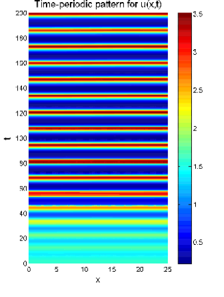
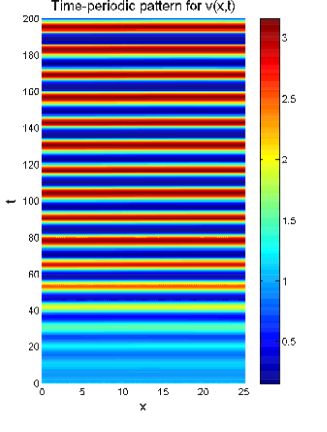
(a)                                                 (b)

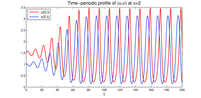
(c)

Figure 1. Numerical simulation of spatially homogeneous time-periodic patterns generated by (5.3) with $\chi(v)=-d^{\prime}(v)$ in the interval $[0,8\pi]$, where $d(v)=d_{1}(v)$ given in (5.18) and parameter values are: $K=4,\gamma=2,\theta=1,\lambda=1,\mu=1,D=1/10$. The initial datum $(u_{0},v_{0})$ is set as a small random perturbation of the homogeneous coexistence steady state $(3/2,1)$. The simulation illustrates a spatially homogeneous time-periodic coexistence patterns for the predator and the prey.

5.3. Spatio-temporal patterns

In this subsection, we shall present some examples to illustrate the periodic and steady state patterns. As discussed in the previous section, the Lotka-Volterra type predator-prey system (5.1) does not generate any spatially inhomogeneous patterns while the Rosenzweig-MacArthur type predator-prey system (5.3) with $\chi(v)=-d^{\prime}(v)$ may generate periodic or steady state patterns in appropriate parameter regimes. Therefore we only consider the Rosenzweig-MacArthur type predator-prey system (5.3) with $\chi(v)=-d^{\prime}(v)$. We fix the value of the parameters in all simulations as follows:

$$K=4,\gamma=2,\theta=1,\lambda=1,\mu=1.$$ (5.17)

Then it can be checked from (5.2) that the coexistence steady state $(u_{*},v_{*})=(3/2,1)$. Furthermore it can be verified from (5.9) that

$$\beta_{1}=\frac{1}{8},\ \beta_{3}=\frac{3}{8}$$

where the value of $\beta_{2}$ depend on the specific form of $d(v)$. In this paper, we shall test three motility function $d(v)$ as follows

$$d_{1}(v)=\frac{1}{1+e^{2(v-1)}},\ \ \ d_{2}(v)=\frac{1}{1+e^{\frac{1}{10}(v-1)}},\ \ \ d_{3}(v)=\frac{1}{9+e^{2(v-1)}}$$ (5.18)

Hence $d_{1}(v_{*})=d_{2}(v_{*})=1/2$, $d_{3}(v_{*})=\frac{1}{10}$ and $\chi_{1}(v_{*})=-d_{1}^{\prime}(v_{*})=\frac{1}{2},\chi_{2}(v_{*})=-d_{2}^{\prime}(v_{*})=\frac{1}{40}$, $\chi_{3}(v_{*})=-d_{3}^{\prime}(v_{*})=\frac{1}{50}$. Next we shall numerically explore the possible patterns for different choices of $d(v)$ given in (5.18).

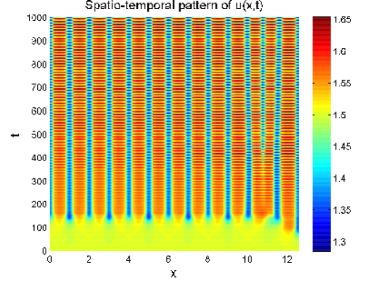
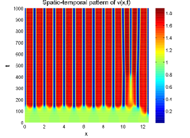
(a)                                                          (b)

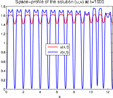
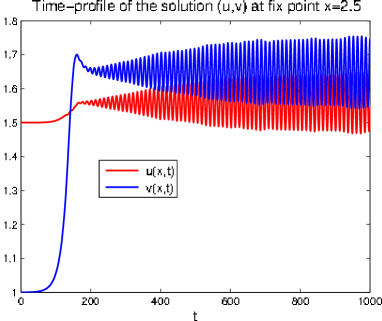
(c)                                                          (d)

Figure 2. Numerical simulation of spatio-temporal patterns generated by (5.3) with $\chi(v)=-d^{\prime}(v)$ in the interval $[0,4\pi]$, where $d(v)=d_{2}(v)$ given in (5.18) and parameter values are: $K=4,\gamma=2,\theta=1,\lambda=1,\mu=1,D=1/4800$. The initial datum $(u_{0},v_{0})$ is set as a small random perturbation of the homogeneous coexistence steady state $(3/2,1)$.

Case 1: $d(v)=d_{1}(v)$. In this case, under the parameters chosen in (5.17), one can verify that

$$a(D,k^{2})=\left(\frac{1}{2}+D\right)k^{2}-\frac{1}{8}.$$ (5.19)

One also can verify from (5.8) that $b(D,k^{2})=\frac{D}{2}k^{4}+\frac{5}{16}k^{2}+\frac{3}{8}>0$, $\beta_{2}=-\frac{5}{16}$ and

$$\Delta=|a(D,k^{2})|^{2}-4b(D,k^{2})=\Big{(}\frac{1}{2}-D\Big{)}^{2}k^{4}-\frac{1}{4}\Big{(}\frac{11}{2}+D\Big{)}k^{2}-\frac{95}{64}.$$

This indicates that as long as $D$ is close to $1/2$, then $\Delta<0$ and Hopf bifurcation will certainly arise. One is concerned whether the steady state bifurcation will occur in this case. Indeed it can be readily checked $a(D,k^{2})<0\ \text{and}\ |a(D,k^{2})|^{2}-4b(D,k^{2})>0$ can not be fulfilled simultaneously. Hence from (5.14), we know that the steady state bifurcation is impossible in this case. However the Hopf bifurcation will develop if $D$ is suitably chosen so that $\Delta<0$ for some $k$. For simulation, we choose $D=1/10$ such that $\Delta<0$ and $a(D,k^{2})<0$ with allowable wavenumber satisfying $k^{2}<\frac{5}{24}$ which, under the facts $k^{2}=(\frac{n\pi}{\ell})^{2},n=0,1,2,\cdots$ with $\ell=8\pi$, gives $n=0,1,2,3$. The numerical simulations of patterns are then shown in Fig.1(a)-(b) where we observe the spatially homogeneous time-periodic patterns. In principle there will be three spatial modes arising from the homogeneous coexistence steady state $(3/2,1)$, but we do not obverse the spatial inhomogeneity. This implies from the plot in Fig.1(c) that as the solution amplitude become large as time increases, the nonlinearity will play a dominant role and the linearized dynamics is insufficient to explain the nonlinear behavior.

Case 2: $d(v)=d_{2}(v)$. For this case, $\beta_{2}=\frac{7}{160}>0$ and $a(D,k^{2})$ is still given by (5.19). Hence the condition (5.15) is verified and

$$\Lambda=\beta_{2}^{2}-4\beta_{3}Dd(v_{*})=\left(\frac{7}{160}\right)^{2}-\frac{3}{4}D.$$

Clearly $\Lambda>0$ if $D<\frac{49}{19200}$ and $\Lambda\leq 0$ if $D\geq\frac{49}{19200}$, which indicates from (5.16) that the steady state bifurcation will occur if $0<D<\frac{49}{19200}$. This is confirmed by numerical simulations shown in Fig. 2 where we take $D=\frac{1}{4800}$ and observe the development of spatially inhomogeneous stationary patterns (see Fig. 2 (a)-(b)). Furthermore both the predator and the prey reach a perfect inhomogeneous coexistence state in space (see Fig.2(c)) but remain oscillations in time (see Fig.2(d)). It has been proved that if $d(v)$ is constant, the diffusive Rosenzweig-MacArthur predator-prey system (5.3) will not admit spatial patterns (cf. [47, 48]). The spatially inhomogeneous stationary patterns shown in Fig.2 implies that density-dependent nonlinear motility (i.e., function $d(v)$), which leads to a cross-diffusion motion, is a trigger for pattern formation. This is a new observation although it is not justified in the paper. When $d(v)$ is constant, the spatial patterns and time-periodic patterns have been obtained for preytaxis systems with different predator-prey interactions or mobility coefficient $\chi(v)$, see [42, 44]. We also refer to [27, 16] for some other types of cross-diffusion which cause the emergence of spatial patterns.

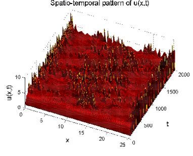
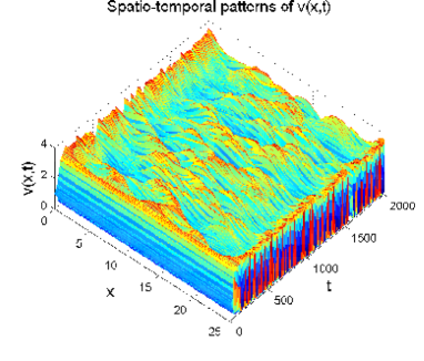
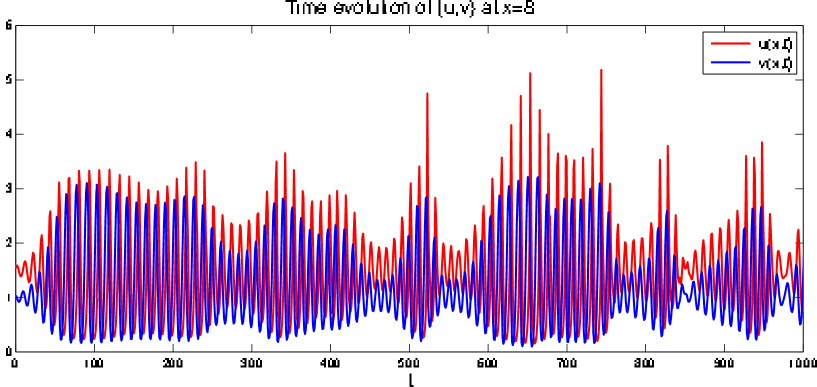
Figure 3. Numerical simulation of spatio-temporal patterns generated by (5.3) with $\chi(v)=-d^{\prime}(v)$ in the interval $[0,8\pi]$, where $d(v)=d_{3}(v)$ given in (5.18) and parameter values are: $K=4,\gamma=2,\theta=1,\lambda=1,\mu=1,D=1/10$. The initial datum $(u_{0},v_{0})$ is set as a small random perturbation of the coexistence steady state $(3/2,1)$.

Case 3: $d(v)=d_{3}(v)$. In this case, one has $d(v_{*})=\frac{1}{10}$ and $\chi(v_{*})=\frac{1}{50}$. Furthermore

$$a(D,k^{2})=(\frac{1}{10}+D)k^{2}-\frac{1}{8},\ b(D,k^{2})=\frac{D}{10}k^{4}+\frac{1}{400}k^{2}+\frac{3}{8}$$

and hence

$$\Delta=|a(D,k^{2})|^{2}-4b(D,k^{2})=\left(\frac{1}{10}-D\right)^{2}k^{4}-\frac{1}{4}\left(\frac{7}{50}+D\right)k^{2}-\frac{95}{64}.$$

Choosing $D=\frac{1}{10}$, then $\Delta<0$ and $a(D,k^{2})<0$ with allowable wavenumber $k^{2}<\frac{5}{8}$. Hence allowable wave modes are $n=0,1,2,3,4,5,6$ by noticing that $k=\frac{n}{8}$ and Hopf bifurcation (with positive real part in the temporal eigenvalue) will arise. We show the numerical simulation in Fig.3, where we observe the development of chaotic spatio-temporal patterns, which are different from the patterns shown in Fig.1 and Fig.2. They are not the periodic patterns either (see the lower panel of Fig.3) as we expect from the linear stability analysis, which indicates again that the dynamics between nonlinear and linearized systems are quite different. We also note that the simulations in Fig.1 and Fig.3 demonstrate that the Hopf bifurcation arising from the time-periodic orbits can develop into spatially homogeneous time-periodic patterns (Fig.1) or chaotic spatio-temporal patterns (Fig.3). The difference in the simulations shown in Fig.1 and Fig.3 lies in the choice of motility function $d(v)$. This observation hints us that the motility function $d(v)$ of the predator plays an important role in determining the spatial distribution of the predator and the prey. In particular the random motion ($d(v)$ is constant) and nonrandom motion ($d(v)$ is non-constant) will result in different patterns (i.e. spatial distribution of the predator and the prey). Hence how does the motility function $d(v)$ affects the dynamics of nonlinear predator-prey systems launches an interesting question for the future.

Acknowledgment. The authors are grateful to the three referees and one editor for their valuable comments, which greatly improved the exposition of our paper. The research of H.Y. Jin was supported by the NSF of China No. 11871226 and the Fundamental Research Funds for the Central Universities. The research of Z. Wang was supported by the Hong Kong RGC GRF grant No. PolyU 153298/16P.

References

- [1] N.D. Alikakos, bounds of solutions of reaction-diffusion equations. Comm. Partial Differential Equations, 4:827-868, 1979.
- [2] B.E. Ainseba, M. Bendahmane, and A. Noussair, A reaction-diffusion system modeling predator-prey with prey-taxis. Nonlinear Anal. Real World Appl.,9(5):2086-2105, 2008.
- [3] H. Amann, Dynamic theory of quasilinear parabolic equations III. Global existence. Math. Z., 202:219-250, 1989.
- [4] H. Amann, Dynamic theory of quasilinear parabolic equations II. Reaction-diffusion systems. Differ. Integral Equ., 3(1):13-75, 1990.
- [5] H. Amann, Nonhomogeneous linear and quasilinear elliptic and parabolic boundary value problems. In Function spaces, differential operators and nonlinear analysis (Friedrichroda, 1992), volume 133 of Teubner-Texte Math., pages 9-126. Teubner, Stuttgart, 1993.
- [6] A. Chakraborty, M. Singh, D. Lucy, and P. Ridland, Predator-prey model with prey-taxis and diffusion. Math. Comp. Mod., 46:482-498, 2007.
- [7] P. Chesson and W. Murdoch, Aggregation of risk: relationships among host-parasitoid medels. Am. Nat., 127:696-715, 1986.
- [8] C. Cosner, Reaction-diffusion-advection models for the effects and evolution of dispersal. Discrere. Contin. Dyn. Syst., 34:1701-1745, 2014.
- [9] E. Curio. The Ethology of Predation. Spring -Verlag, New York, 1976.
- [10] X. Fu, L.-H. Tang, C. Liu, J.-D. Huang, T. Hwa and P. Lenz, Stripe formation in bacterial system with density-suppressed motility. Phys. Rev. Lett., 108:198102, 2012.
- [11] D. Grünbaum, Using spatially explicit models to characterize foraging performance in heterogeneous landscapes. Am. Nat., 151:97-115, 1998.
- [12] C.S. Holling, The functional response of predators to prey density and its role in mimicry and population regulation. Mem. Entom. Soc. Can., 45:1-60, 1965.
- [13] H.Y. Jin and Z.A. Wang, Global stability of prey-taxis systems. J. Differential Equations, 262:1257-1290, 2017.
- [14] H.Y. Jin, Y.J. Kim and Z.A. Wang, Boundedness, stabilization and pattern formation driven by density-suppressed motility. SIAM J. Appl. Math., 78:1632-1657, 2018.
- [15] A. Jüngel, Diffusive and Nondiffusive Population Models. Mathematical modeling of collective behavior in socio-economic and life sciences, 397-425, Model. Simul. Sci. Eng. Technol., Birkhäuser Boston, Inc., Boston, MA, 2010.
- [16] A. Jüngel, C. Kuehn and L. Trussardi, A meeting point of entropy and bifurcations in cross-diffusion herding. European J. Appl. Math., 28(2):317-356, 2017.
- [17] P. Kareiva and G.T. Odell, Swarms of predators exhibit “preytaxis” if individual predators use area-restricted search. Am. Nat., 130:233-270, 1987.
- [18] E.F. Keller and L.A. Segel, Model for chemotaxis. J. Theor. Biol., 30(2):225-234,1971.
- [19] W.G. Kelley and A.C. Peterson, The Thoery of Differential Equations - Classical and Qualitative, Springer, 2010.
- [20] R. Kowalczyk and Z. Szymańska, On the global existence of solutions to an aggregation model. J. Math. Anal. Appl., 343:379-398, 2008.
- [21] O. Ladyzhenskaya, V. Solonnikov, and N. Uralceva, Linear and Quasilinear Equations of Parabolic Type. AMS, Providence, RI, 1968.
- [22] J.P. LaSalle, Some extensions of Lyapunov’s second method. IRE Transactions on Circuit Theory, CT-7, 520-527, 1960.
- [23] J.M. Lee, T. Hillen, and M.A. Lewis, Continuous travling waves for prey-taxis. Bull. Math. Biol., 70:654-676, 2008.
- [24] J.M. Lee, T. Hillen, and M.A. Lewis, Pattern formation in prey-taxis systems. J. Biol. Dyn., 3(6):551-573, 2009.
- [25] C. Liu et al. Sequtential establishment of stripe patterns in an expanding cell population. Science, 334:238-241, 2011.
- [26] A.J. Lotka, Elements of Physical Biology. Baltimore: Williams and Wilkins Co., 1925.
- [27] M. Mimura and K. Kawasaki, Spatial segregation in competitive interaction-diffusion equations. J. Math. Biol., 9(1):49-64, 1980.
- [28] N. Mizoguchi and P. Souplet, Nondegeneracy of blow-up points for the parabolic Keller-Segel system. Ann. Inst. H. Poincaré Anal. Non Linéaire, 31:851-875, 2014.
- [29] W.W. Murdoch, C.J. Briggs, and R.M. Nisbert, Consumer-Resource Dynamics (Monographs in Population Biology-36). Princeton University Press, 2003.
- [30] W. Murdoch, J. Chesson, and P. Chesson, Biological control in theory and practice. Am. Nat., 125:344-366, 1985.
- [31] A. Okubo and S.A. Levin, Diffusion and Ecological Problems: Modern Perspective. Interdisciplinary Applied Mathematics, vol. 14. 2nd ed. Berlin: Springer, 2001.
- [32] M.M. Porzio and V.Vespri, Hölder estimates for local solutions of some doubly nonlinear degenerate parabolic equations. J. Differential Equations, 103(1):146-178, 1993.
- [33] M.L. Rosenzweig and R.H. MacArthur, Graphical representation and stability conditions of predator-prey interactions. Am. Nat., 97:209-223, 1963.
- [34] N. Sapoukhina, Y. Tyutyunov, and R. Arditi, The role of prey taxis in biological control: a spatial theoretical model. Am. Nat., 162:61-76, 2003.
- [35] J. Smith-Roberge, D. Iron and T. Kolokolnikov, Pattern formation in bacterial colonies with density-dependent diffusion. European J. Appl. Math., 30(1):196-218, 2019.
- [36] P. Souplet and P. Quittner, Superlinear Parabolic Problems: Blow-up, Global Existence and Steady States. Birkhäuser Advanced Texts, Basel/Boston/Berlin, 2007.
- [37] Y.S. Tao, Global existence of classical solutions to a predator-prey model with nonlinear prey-taxis. Nonlinear Anal. Real World Appl., 11(3):2056-2064, 2010.
- [38] Y.S. Tao and M. Winkler, A chemotaxis-haptotaxis model: the roles of nonlinear diffusion and logistic source. SIAM J. Math. Anal., 43(2):685-704, 2011.
- [39] Y.S. Tao and M. Winkler, Boundedness in a quasilinear parabolic-parabolic Keller-Segel system with subcritical sensitivity. J. Differential Equations, 252(1):692-715, 2012.
- [40] P. Turchin, Complex Population Dynamics: A Theoretical/Empirical Synthesis (Monographs in Population Biology-35). Princeton University Press, 2003.
- [41] V. Volterra, Fluctuations in the abundance of a species considered mathematically. Nature, 118:558-560, 1926.
- [42] K. Wang, Q. Wang and F. Yu, Stationary and time periodic patterns of two predator and one-prey systems with prey-taxis. Discrere. Contin. Dyn. Syst., 37(1):505-543, 2017.
- [43] M.X. Wang, Note on the Lyapunov functional method. Appl. Math. Lett., 75:102-107, 2018.
- [44] Q. Wang, Y. Song and L.J. Shao, Nonconstant positive steady states and pattern formation of 1D prey-taxis systems. J. Nonlinear Sci., 27(1):71-97, 2017.
- [45] J.P. Wang and M.X.Wang, Boundedness and global stability of the two-predator and one-prey models with nonlinear prey-taxis. Z. Angew. Math. Phys., 69(3): 63, 24pp, 2018.
- [46] S. Wu, J.P. Shi, and B. Wu, Global existence of solutions and uniform persistence of a diffusive predator-prey model with prey-taxis. J. Differential Equations, 260(7):5847-5874, 2016.
- [47] S. Wu, J Wang and J. Shi, Dynamics and pattern formation of a diffusive predator-prey model with predator-taxis. Math. Models Method Appl. Sci., 28(11):2275-2312, 2018.
- [48] F. Yi, J. Wei and J. Shi, Bifurcation and spatiotemporal patterns in a homogeneous diffusive predator-prey system, J. Differential Equations, 246:1944-1977, 2009.