Particles in turbulent separated flow over a bump: effect of the Stokes number and lift force
Abstract
Particle-laden turbulent flow that separates due to a bump inside a channel is simulated to analyse the effects of the Stokes number and the lift force on the particle spatial distribution. The fluid friction Reynolds number is approximately 900 over the bump, the highest achieved for similar computational domains. A range of particle Stokes numbers are considered, each simulated with and without the lift force in the particle dynamic equation. When the lift force is included a significant difference in the particle concentration, in the order of thousands, is observed in comparison with cases where the lift force is omitted. The greatest deviation is in regions of high vorticity, particularly at the walls and in the shear layer but results show that the concentration also changes in the bulk of the flow away from the walls. The particle behaviour changes drastically when the Stokes number is varied. As the Stokes number increases, particles bypass the recirculating region that is formed after the bump and their redistribution is mostly affected by the strong shear layer. Particles segregate at the walls and particularly accumulate in secondary recirculating regions behind the bump. At higher Stokes numbers, the particles create reflection layers of high concentration due to their inertia as they are diverted by the bump. The fluid flow is less influential and this enables the particles to enter the recirculating region by rebounding off walls and create a focus of high particle concentration.
I Introduction
Turbulent flows laden with particles are common in natural phenomena and engineering applications. The understanding of turbulence and multiphase flows is considered a challenge in both experiments and numerical simulations Balachandar and Eaton (2010); Elghobashi (2019). As for single-phase flow simulations, different formulations for the carrier phase in multiphase flows can be used such as direct numerical simulation (DNS), the method used here, large-eddy simulation (LES), Marchioli (2017); Innocenti, Marchioli, and Chibbaro (2016); Park et al. (2017), or Reynolds-averaged Navier-Stokes equations (RANS), Minier, Chibbaro, and Pope (2014); Sajjadi et al. (2017); Vahidifar, Saffarian, and Hajidavalloo (2018).
To these possible descriptions of turbulent flow, Lagrangian methods can be used to couple particles and fluid at different levels, i.e. one-way, two-way or four-way coupling regime, Elghobashi (1994). In the one-way coupling the particle volume fraction and mass loading are low, the particles are transported by the carrier phase which is not modified. For higher mass loading and small volume fraction, two-way coupling considers the flow modulation due to the particles. In four-way coupling, collisions and hydrodynamic interaction between particles are significant.
In simulations involving a large number of particle smaller than the Kolmogorov scale, a suitable numerical approach is the Lagrangian point-particle method, Toschi and Bodenschatz (2009); Kuerten (2016). In such mixed Eulerian-Lagrangian method, the continuous phase is described in a Eulerian framework whilst the dispersed phase by a Lagrangian approach solving the dynamic equation for each particle. Particles may be considered to be spherical or, requiring more complex modelling, non-spherical particles may be considered Gustavsson et al. (2017); Voth and Soldati (2017).
The study of particle-laden turbulent flow has been of interest for decades by considering isotropic turbulence, Squires and Eaton (1991); Bragg, Ireland, and Collins (2015), and homogeneous shear turbulence, Nicolai et al. (2014); Battista et al. (2018), and cases where the flow is confined by solid boundaries to investigate, for example, particle behaviour in turbulent boundary layers, Sardina et al. (2011, 2012a); Li et al. (2016) or in Couette flow Bernardini, Pirozzoli, and Orlandi (2013). Various studies are conducted in wall-bounded flows, Marchioli et al. (2008), and they include confined flows such as pipe flows, Marchioli et al. (2003); Picano, Sardina, and Casciola (2009) and channels, Sardina et al. (2012b); Kulick, Fessler, and Eaton (1994), sometimes with the addition of roughness on the surface of the channel’s walls to modulate the flow and hence the particle dynamics, Liu, Luo, and Fan (2016); De Marchis et al. (2016); Vreman (2015). The study of particle-laden fluid jets is also active due to their vast use in engineering and their occurrence in nature, Picano et al. (2011); Gualtieri, Battista, and Casciola (2017); Battista et al. (2011); Wu et al. (2017). Some studies focus, for example, on the effect of the Stokes number on particle behaviour in turbulent jets, both experimentally Lau and Nathan (2014, 2016) and numerically Wang, Zheng, and Wang (2017).
In many applications though, the geometry involved is more complex than these standard domains. For example, microparticles are used in inhalable drug delivery systems since they provide a non-invasive treatment and localised delivery method. Some authors Abdelaziz et al. (2017) discuss their use in the treatment of lung cancer whilst other Ni et al. (2017) show how microparticles can be used to deliver embedded nanocrystals to the lungs. These applications call for numerical simulations to study microparticle behaviour in realistic models of human airways Ghahramani et al. (2017); Stylianou, Sznitman, and Kassinos (2016) together with the effect of different breathing conditions Rahimi-Gorji et al. (2015). Another health related example is the obstruction in blood vessels due to atherosclerosis which is nowadays also studied with the aid of computational modelling Thondapu et al. (2016); Choi et al. (2018).
A geometrical change may be intentional, for example, to enhance mixing of fluid and particles or to separate particles from fluid for filtration. Specific geometries can be used for the preferential separation of particles when populations of particles with different characteristics are present in a carrier phase. In Refs. Huang and Durbin (2010, 2012) the authors study particulate dispersion and mixing through DNS in a serpentine channel by considering a large range of particle Stokes numbers. The authors observe high concentrations of particles near the surface of the outer wall and show how the heaviest particles reflect from the wall to form reflection layers whilst the lighter particles concentrate in the streaks at the wall. A recent study Noorani et al. (2015) also observe particle reflections in the outer bend of turbulent curved pipe flow laden with micro-sized inertial particles. The authors document the modification of particle axial and wall-normal velocities and the increase in particle turbulent kinetic energy. Other studies Ault et al. (2016) show the importance of geometry for particle-capture mechanisms in branching junctions by comparing experiments and numerical simulations. The authors show that the capture is dependent on vortex breakdown, a result of the creation and evolution of recirculating regions in the system and a crucial factor that determines whether particle accumulation is maximised or eliminated.
The aim of the present paper is to study the microparticles behaviour in a turbulent channel flow with bump at one of the walls by means of a Lagrangian point-particle method in an incompressible flow simulated using DNS. The bump makes the flow separate, creating a strong shear layer and recirculating region, Stella, Mazellier, and Kourta (2017); Krank, Kronbichler, and Wall (2017); Schiavo, Wolf, and Azevedo (2017). The configuration is nonetheless still accessible to classical statistical tools and turbulence theory for the detailed study of turbulence dynamics, Mollicone et al. (2018, 2017); Passaggia and Ehrenstein (2018); Kähler, Scharnowski, and Cierpka (2016). To the best of our knowledge, this is the first simulation of such a configuration laden with particles at a friction Reynolds number of 900 over the bump. A wide range of populations ranging from almost tracers to ballistic particles are addressed. Additionally, due to the high vorticity present in some regions of the flow, we investigate if and where the lift force significantly influences the particle dynamics.
II Simulation Setup
II.1 Fluid phase
The computational domain has dimensions , where , , and are the streamwise, wall-normal and spanwise coordinates respectively and is half the nominal channel height, see figure 1. Periodic boundary conditions are enforced in both and directions, whilst at the walls no-slip conditions are applied. The bottom wall contains a bump that is described by the easily reproducible and differentiable equation (especially important for particle rebound) where , , and ranges from to . The periodicity in the streamwise direction avoids artificial inflow/outflow boundary conditions and the period is chosen as large as possible, within computational limitations, to allow the analysis of an almost isolated bump, with definite flow reattachment and negligible streamwise correlation. The incoming flow accelerates at the channel restriction and a recirculating region forms behind the bump, starting downstream of the bump tip. An intense shear layer separates the recirculating region from the outer flow. Downstream of the bump, the flow re-attaches completely. The turbulence dynamics for such flows over a bump is discussed in detail in Mollicone et al. (2017, 2018).
Direct numerical simulation (DNS) is used to solve the incompressible Navier-Stokes equations,
| (1) |
where is the fluid velocity, is the time, is the hydrodynamic pressure and is the kinematic viscosity. Nek5000 Fischer, Lottes, and Kerkemeier (2008), which is based on the spectral element method (SEM) Patera (1984), is used to solve both the flow domain and the dispersed phase. The implemented algorithm for the computation of the particle dynamics is deeply described in subsection II.2. The simulations are carried out at bulk Reynolds number , where is the bulk velocity. All length scales are made dimensionless with the nominal channel half-height , time with and pressure with . The maximum friction Reynolds number, achieved close to the bump tip, is , defined as , where the friction velocity is , is the local mean shear stress and is the constant fluid density. The simulation has been performed with about million grid point on cores using approximately million core hours, using spectral elements of order of . In this case the grid spacing, , and , is adeguate for the high fidelity description of all the flow scales. For detailed discussion about the resolution the reader can refer to section 2 of Ref. Mollicone et al. (2017). Approximately 500 statistically uncorrelated fields, separated by a time interval of , have been collected for each simulation in order to obtain properly converging statistics. Defining the ’flow-through time’, , as the time needed for a turbulent structure to travel all along the channel length, the simulation time is , which makes sure that statistics converge.
II.2 Solid phase
The solid phase is composed of spherical particles with radius smaller than the dissipative scale, the wall unit in our case. In a dilute suspension at low mass loading, the turbulence modulation due to the particles, the inter-particle collisions and the hydrodynamic interactions can be neglected Balachandar and Eaton (2010). Under these conditions, the one-way coupling regime can be assumed and the Newton equation is forced by the Stokes drag together with the lift force which we intentionally include or omit to investigate its effect, namely
| (2) |
where is the particle position, is the particle velocity, is the fluid velocity at the particle position and is the particle relaxation time, is the particle to fluid density ratio, is the particle diameter, the coefficient of the lift force is and is the vorticity. The particles elastically bounce at the wall, where in correspondence of the bump the exact bouncing direction is evaluated by the analytical function of the wall profile.The dynamics of the particle in the one-way coupling regime is well described by the Stokes number, i.e. the ratio between the particle relaxation time and the fluid characteristic time scale. Two different Stokes numbers are defined, the reference one, , and the viscous Stokes number, . The two are related through the Reynolds number, .
Equations (2) are evolved for each single particle with a fourth order Adams-Bashforth method in time. A spectral interpolation, intrinsic to the Nek5000 code, is employed to evaluate the fluid variables at the particle position. Twenty different populations are evolved: ten different Stokes numbers each with and without the lift term. Ten million of particle are considered in the simulation. The huge number of particles is employed to obtain an adeguate statistical convergence, since each single particle does not feel the presence of the other and does not modify the carrier flow. The effect of gravity is negligible for the particle population considered in the present study. In fact, the dimensionless terminal velocity, , can be expressed in terms of the control parameters as where is the bulk Froude number. For the heaviest population at , it turns out that the ratio is of the order of .
III Results
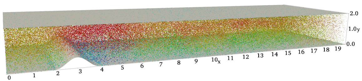
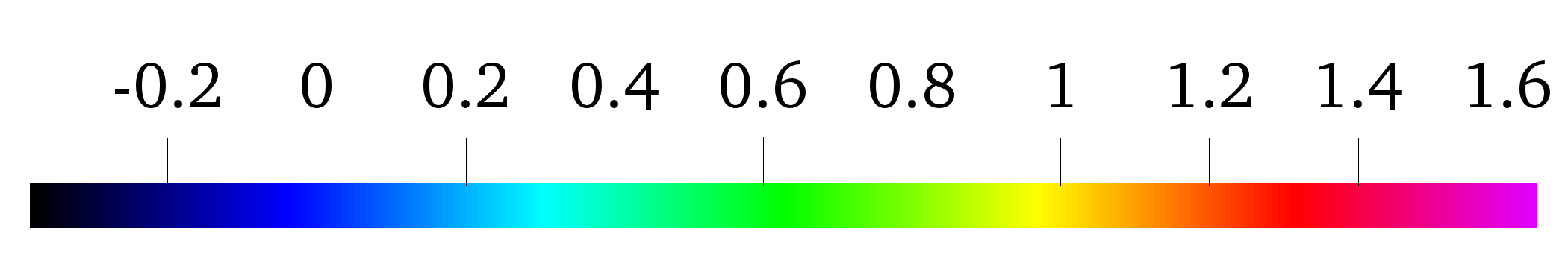
Figure 1 shows instantaneous snapshots of the particles coloured with their instantaneous streamwise velocity for . The whole computational domain is shown in the left panels whilst the area around the bump, in a view orthogonal to the - plane, is shown in the right panels. Unless otherwise stated, figures show the particles that have been evolved with the lift term included in equation (2). At low Stokes number, the particles distribute themselves evenly throughout the domain and have velocities comparable to the fluid velocity. The low particle velocity inside the recirculating region behind the bump contrasts the high particle velocity at the centre of the channel. On the other hand, at , the number of particles in the recirculating region is negligible. The particles move towards the upper part of the channel as they are projected upwards as they hit the bump. At higher Stokes number, the particles have a ballistic motion and after hitting the bump continue to bounce off the upper wall and therefore manage to enter the recirculating region. Particles that do not hit the bump continue straight in their trajectory, as shown by the particles above behind the bump.
![[Uncaptioned image]](/html/1907.02270/assets/FIGURES/conc_2YL_02_St1_ZOOM.png)
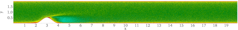
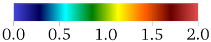
The particle behaviour is discussed in detail by considering the mean particle concentration, , where is the instantaneous local number of particles in a cell at position, is the corresponding cell volume, is the total number of particles and is the total domain volume. The angular brackets denote averaging in the homogeneous spanwise direction, , and in time. The normalisation by represents the homogeneous particle concentration, i.e. the concentration value that would be obtained at any point if all the particles were equally distributed in all the domain. The data sets are taken after the system is statistically stationary and at time intervals larger than the correlation time. Six out of the total ten particle populations that have been simulated, , will be presented since the populations that exhibit similar behaviour are omitted. The population at is omitted since particles act as tracers and fill the whole domain homogeneously with no effect of the bump and only a slight accumulation at the walls. Figures 2 and LABEL:fig:conc_zoom show the mean particle concentration as a coloured contour plot, with the latter zoomed on the region around the bump since it is the area of interest.
At , some particles segregate towards the channel walls whilst a homogenous concentration, indicated by the green colour, is present in most of the domain. The concentration increases at the bump wall, particularly in three locations: before the bump, just after the tip of the bump and after the bump. These locations coincide with three small recirculating bubbles that form in the fluid, see the zero velocity isoline in figure 5(a), that capture the particles. Figure 4 shows line plots of mean particle concentration at these locations, specifically at . away from the walls for all three positions, confirming the homogeneous distribution. The concentration increases to the order of 10 at the top wall and order 100 at the bottom wall, both before and after the bump, panels (a) and (c). In the latter, the particles manage to enter the recirculating region and the concentration only decreases slightly with respect to up to . A more pronounced decrease, even though the particles are still clearly present, can be seen further behind the bump, but still in the recirculating region, shown by the cyan colour in figure LABEL:fig:conc_zoom(a). Just after the tip of the bump, the particles are affected by the shear layer forming in the fluid. Figure 5(b) shows the turbulent kinetic energy production , where angular brackets and apices indicate the mean and the fluctuations, respectively. The high value of indicates the location and intensity of the shear layer. Figure 4 reports the wall normal profiles of the particle concentration at different streamwise position, in particularpanel (b) refers to a streamwise position that traverses the shear layer. The plot shows the accumulation of particles at the bump wall, , up to . These are the particles that move up the bump wall and towards the tip, since they follow the fluid which is recirculating under the shear layer behind the bump, see the negative particle velocity in figure 1(b) and the region of negative fluid velocity in figure 5(a). As the shear layer is encountered, the concentration slightly drops below that is reached when moving further away from the shear layer and towards the center of the channel. For particles having this Stokes number, the effect of the lift is negligible.
At , see figure 2(b) and the zoom in figure LABEL:fig:conc_zoom(b), the particle behaviour is similar to the one for , except for the significant decrease in concentration away from the walls which is compensated by an increase at the walls. The concentration also decreases in the stream above the shear layer with respect to the previous Stokes number. The inertia of the particles increases with Stokes number and consequently less particles are capable of entering the recirculating region. The increased particle segregation towards the wall persists downstream of the bump where , and it is more intense than the lower Stokes number case.
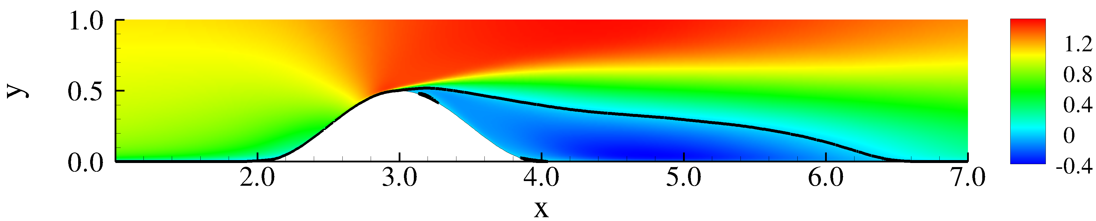
When the Stokes number is increased to , figures 2(c) and LABEL:fig:conc_zoom(c), the particles segregate more towards the walls and have a low concentration (dark blue) in the rest of the domain. The main recirculating region behind the bump contains no particles (purple colour) except for concentrations of particles in the two, small, secondary recirculating bubbles at the walls (discussed for ). A high concentration of particles, in the order of a thousand times the homogeneous value, is present before the bump, at the wall (). The concentration is high along the bump wall (left side) up to the bump’s tip, after which the particles are projected towards the centre of the channel by the flow and transported downstream. Figure 6 shows the mean particle concentration at . In general, a slight difference in concentration appears when the lift term is included or not, except for an evident deviation from the two values in the shear layer, see panel (b) at . The strong vorticity present in the shear layer, which influences the lift, is a direct responsible for this discrepancy. Panel (c) shows that the concentration is low in the recirculating region, , but nonetheless high at both walls, even if the bottom wall is underneath a region containing no particles. The particles must therefore reach this region from the edge of the recirculation where the flow reattaches and they are transported towards the left along the wall by reverse (upstream) flow.
At higher Stokes numbers, the particles’ inertia becomes dominant and therefore their response to the flow is minimal. Figures 2(d), (e) and (f), together with the corresponding panels in figure LABEL:fig:conc_zoom, show the concentration for . After hitting the bump and being projected upwards, the particles proceed towards the upper wall. At , the stream of particles still bends downwards towards the centre of the channel, since the mean flow has some effect on them since the characteristic time of the mean flow is comparable with the particle relaxation time which in turn is sensibly larger than the fluctuation characteristic time. At , the stream starts resembling a straight line and the rebound of particles at the upper wall starts to show. Once they rebound, , the flow re-directs them in the streamwise direction and the particles do not enter the recirculating region from above. This is not the case for the highest Stokes number, , since the particles are almost entirely inertial and, after bouncing off the top wall, proceed into the recirculating region and create a focused region of high concentration at close to the bottom wall. The focusing is possible due to the particles hitting the rounded shape of the bump on its right-hand side. The particles then spread out back into the channel, depending on the angle at which they hit the bump which is a consequence of the angle at which they would have bounced off the top wall from the stream coming from the left-hand side of bump. As they initially hit the bump, the particles create a reflection layer, a term coined by Huang and Durbin (2012), which resembles a shockwave since the population of particles act as a compressible phase. The particles segregate towards the upper part of the channel for these higher Stokes numbers. Apart from the particles that are projected upwards by the bump, another contribution to this segregation is due to the particles that travel at and therefore continue in their trajectory without hitting the bump, with only a minimal effect of the turbulent fluctuations that are not able to re-distribute them into all the domain as with the particles at lower Stokes numbers.
Figure LABEL:fig:nofluid_mean shows to what extent the particle stream is affected by the mean flow or the turbulent flow at these higher Stokes numbers. Panels (a) and (b) show and respectively with the colour contour representing the mean particle concentration for the fully turbulent DNS simulation as in panels (e) and (f) in figure LABEL:fig:conc_zoom. The white iso-surface shows the particle concentration of a separate simulation when there is no coupling, i.e. the particle acceleration is zero and only the rebound from the solid walls is considered. Note that the white iso-contours are identical in both panels since the dynamics is independent of the Stokes number (no fluid interaction). The particles are given an initial streamwise velocity and the ones travelling at hit the bump and create a well-defined reflection layer that bounces off the top wall and then the right-hand side of the bump (). Concentration of particles close to the wall at is still observed due to the other particles that bounce off the top wall, reflect along the back of the bump () and focus in this small region. The black iso-surface shows the particle concentration when they are coupled with only the mean flow (no fluctuations) obtained from the turbulent simulation. At , the black iso-contour departs from the white one both after the particles are deflected by the bump and, most notably, after they bounce off the top wall, disappearing well above the recirculating region. This shows that the mean flow still affects the particles by shifting them in the streamwise direction and stops them from entering the recirculation. On the other hand, at , the effect of the mean flow is less pronounced. After the deflection by the bump, the three contours are almost superimposed. After bouncing off the top wall the black iso-contour is slightly deflected but now manages to enter the recirculating region. The particles bounce off the bump wall and focus at , superimposing the white and coloured contours. The turbulent fluctuations therefore play an important role by deviating the particle stream or dispersing it. Nonetheless, in high Stokes number cases, considering only the mean flow for particle transport, the qualitative behaviour is well predicted.
![[Uncaptioned image]](/html/1907.02270/assets/FIGURES/conc_meanflow_noflow_St200.png)
The lift force plays a crucial role in determining the particle concentration at , see figure 8. Away from the walls, the concentration for the particles without the lift is approximately half the one for particles with the lift and therefore the lift cannot be considered to be negligible, see panels (a) and (b) for plots taken at and respectively. This concentration difference is balanced by a surprising change in concentration at the walls. Panel (c) shows the detail in very close proximity of the wall at as an example. The concentration for the particles with the lift force is hundreds of times lower than those with no lift force. Even though this only occurs in a small region close to the wall, the significant quantitative difference together with the importance of particle segregation at the wall confirms the importance of the lift force. This difference can be again attributed to vorticity which is strong in this region due to the presence of the bounding wall. The particles migrating towards the walls experience a negative slip velocity with respect to the fluid, and a negative fluid vorticity at the bottom wall (positive at the top wall), producing a net lift force towards the center of the channel, which prevents the particle wall segregation.
The number of particles at the bottom wall under the recirculating region () also decreases significantly compared to the lower Stokes numbers, see figure 9(a). The reverse flow on the right of the recirculating region is not able to capture as many particles as previously seen for the lower Stokes numbers since the particles’ inertia is now higher. When the Stokes increases to , see panel (b), no particles are captured and the concentration at is practically zero. On the other hand, at , see panel (c), there is a concentration peak inside recirculating region due to the particles bouncing off the upper wall and focusing in this region, as discussed previously. The difference in particle concentration with or without the lift force disappears away from the walls as the Stokes number is increased but still persists at the top wall where particles with lift force have significantly less concentration.
IV Final remarks
The effects of Stokes number and lift force have been analysed for particle-laden turbulent flow that separates due to the presence of a bump in a channel-like domain. A strong shear layer and a recirculating region are formed behind the bump, both affecting the particle dynamics. The Reynolds number is relatively high when considering similar geometries and the present multi-phase configuration has, to the best of our knowledge, never been simulated before.
A vast range of Stokes numbers are considered, simulated both with and without the lift force in the particle dynamic equation. The conclusion is that the lift force must not be neglected, since there are drastic changes in particle concentration for some Stokes numbers with respect to results obtained without the lift force. Regions of high vorticity, particularly at the walls and in the shear layer, exhibit the greatest differences. However, for some intermediate Stokes numbers, the difference is also evident in the bulk of the flow throughout the whole domain.
The particles behave as tracers at low Stokes numbers and closely follow the fluid phase. As the Stokes number is increased, the particles tend to segregate at the walls and do not enter the recirculating region behind the bump. Some particles are captured by the recirculation, forced upstream as they move close to the wall and transported back downstream as they encounter the strong shear layer formed by the bump. Secondary recirculating regions, one before the bump and two inside the primary recirculating region, manage to capture the particles. At the highest Stokes numbers, the particles’ inertia is high and their ballistic nature makes them bounce off the bump, top and bottom walls, creating reflection layers as they are only slightly affected by the fluid flow. This enables the particles to enter the recirculating region by bouncing off the back of the bump and creating a focused spot of high particle concentration.
Understanding particle-laden flows in presence of features such as a bump is important for engineering applications that concern geometries relatively more complex than classical flows such as straight pipes or planar channels. Such features may be intentional (such as for filtration or separation of particles) or unintentional (such as defects) and it is essential to comprehend how particles, that may have different Stokes numbers, behave in such particle-laden flows.
Acknowledgements.
The research has received funding from the European Research Council under the ERC Grant Agreement no. 339446. We acknowledge CINECA for awarding us access to supercomputing resource MARCONI based in Bologna, Italy through ISCRA project no. HP10BLVPKA.References
- Balachandar and Eaton (2010) S. Balachandar and J. K. Eaton, “Turbulent dispersed multiphase flow,” Annual Review of Fluid Mechanics 42, 111–133 (2010).
- Elghobashi (2019) S. Elghobashi, “Direct numerical simulation of turbulent flows laden with droplets or bubbles,” Annual Review of Fluid Mechanics 51, 217–244 (2019).
- Marchioli (2017) C. Marchioli, “Large-eddy simulation of turbulent dispersed flows: a review of modelling approaches,” Acta Mechanica 228, 741–771 (2017).
- Innocenti, Marchioli, and Chibbaro (2016) A. Innocenti, C. Marchioli, and S. Chibbaro, “Lagrangian filtered density function for les-based stochastic modelling of turbulent particle-laden flows,” Physics of Fluids 28, 115106 (2016).
- Park et al. (2017) G. I. Park, M. Bassenne, J. Urzay, and P. Moin, “A simple dynamic subgrid-scale model for les of particle-laden turbulence,” Physical Review Fluids 2, 044301 (2017).
- Minier, Chibbaro, and Pope (2014) J.-P. Minier, S. Chibbaro, and S. B. Pope, “Guidelines for the formulation of lagrangian stochastic models for particle simulations of single-phase and dispersed two-phase turbulent flows,” Physics of Fluids 26, 113303 (2014).
- Sajjadi et al. (2017) H. Sajjadi, M. Salmanzadeh, G. Ahmadi, and S. Jafari, “Lattice boltzmann method and rans approach for simulation of turbulent flows and particle transport and deposition,” Particuology 30, 62–72 (2017).
- Vahidifar, Saffarian, and Hajidavalloo (2018) S. Vahidifar, M. R. Saffarian, and E. Hajidavalloo, “Introducing the theory of successful settling in order to evaluate and optimize the sedimentation tanks,” Meccanica (2018), 10.1007/s11012-018-0907-2.
- Elghobashi (1994) S. Elghobashi, “On predicting particle-laden turbulent flows,” Applied Scientific Research 52, 309–329 (1994).
- Toschi and Bodenschatz (2009) F. Toschi and E. Bodenschatz, “Lagrangian properties of particles in turbulence,” Annual review of fluid mechanics 41, 375–404 (2009).
- Kuerten (2016) J. G. M. Kuerten, “Point-particle dns and les of particle-laden turbulent flow-a state-of-the-art review,” Flow, turbulence and combustion 97, 689–713 (2016).
- Gustavsson et al. (2017) K. Gustavsson, J. Jucha, A. Naso, E. Lévêque, A. Pumir, and B. Mehlig, “Statistical model for the orientation of nonspherical particles settling in turbulence,” Physical review letters 119, 254501 (2017).
- Voth and Soldati (2017) G. A. Voth and A. Soldati, “Anisotropic particles in turbulence,” Annual Review of Fluid Mechanics 49, 249–276 (2017).
- Squires and Eaton (1991) K. D. Squires and J. K. Eaton, “Preferential concentration of particles by turbulence,” Physics of Fluids A: Fluid Dynamics 3, 1169–1178 (1991).
- Bragg, Ireland, and Collins (2015) A. D. Bragg, P. J. Ireland, and L. R. Collins, “Mechanisms for the clustering of inertial particles in the inertial range of isotropic turbulence,” Physical Review E 92, 023029 (2015).
- Nicolai et al. (2014) C. Nicolai, B. Jacob, P. Gualtieri, and R. Piva, “Inertial particles in homogeneous shear turbulence: experiments and direct numerical simulation,” Flow, turbulence and combustion 92, 65–82 (2014).
- Battista et al. (2018) F. Battista, P. Gualtieri, J.-P. Mollicone, and C. M. Casciola, “Application of the exact regularized point particle method (erpp) to particle laden turbulent shear flows in the two-way coupling regime,” International Journal of Multiphase Flow 101, 113–124 (2018).
- Sardina et al. (2011) G. Sardina, F. Picano, P. Schlatter, L. Brandt, and C. M. Casciola, “Large scale accumulation patterns of inertial particles in wall-bounded turbulent flow,” Flow, turbulence and combustion 86, 519–532 (2011).
- Sardina et al. (2012a) G. Sardina, P. Schlatter, F. Picano, C. M. Casciola, L. Brandt, and D. S. Henningson, “Self-similar transport of inertial particles in a turbulent boundary layer,” Journal of Fluid Mechanics 706, 584–596 (2012a).
- Li et al. (2016) D. Li, A. Wei, K. Luo, and J. Fan, “Direct numerical simulation of a particle-laden flow in a flat plate boundary layer,” International Journal of Multiphase Flow 79, 124–143 (2016).
- Bernardini, Pirozzoli, and Orlandi (2013) M. Bernardini, S. Pirozzoli, and P. Orlandi, “The effect of large-scale turbulent structures on particle dispersion in wall-bounded flows,” International Journal of Multiphase Flow 51, 55–64 (2013).
- Marchioli et al. (2008) C. Marchioli, A. Soldati, J. G. M. Kuerten, B. Arcen, A. Taniere, G. Goldensoph, K. D. Squires, M. F. Cargnelutti, and L. M. Portela, “Statistics of particle dispersion in direct numerical simulations of wall-bounded turbulence: results of an international collaborative benchmark test,” International Journal of Multiphase Flow 34, 879–893 (2008).
- Marchioli et al. (2003) C. Marchioli, A. Giusti, M. V. Salvetti, and A. Soldati, “Direct numerical simulation of particle wall transfer and deposition in upward turbulent pipe flow,” International journal of Multiphase flow 29, 1017–1038 (2003).
- Picano, Sardina, and Casciola (2009) F. Picano, G. Sardina, and C. M. Casciola, “Spatial development of particle-laden turbulent pipe flow,” Physics of Fluids 21, 093305 (2009).
- Sardina et al. (2012b) G. Sardina, P. Schlatter, L. Brandt, F. Picano, and C. M. Casciola, “Wall accumulation and spatial localization in particle-laden wall flows,” Journal of Fluid Mechanics 699, 50–78 (2012b).
- Kulick, Fessler, and Eaton (1994) J. D. Kulick, J. R. Fessler, and J. K. Eaton, “Particle response and turbulence modification in fully developed channel flow,” Journal of Fluid Mechanics 277, 109–134 (1994).
- Liu, Luo, and Fan (2016) X. Liu, K. Luo, and J. Fan, “Turbulence modulation in a particle-laden flow over a hemisphere-roughened wall,” International Journal of Multiphase Flow 87, 250–262 (2016).
- De Marchis et al. (2016) M. De Marchis, B. Milici, G. Sardina, and E. Napoli, “Interaction between turbulent structures and particles in roughened channel,” International Journal of Multiphase Flow 78, 117–131 (2016).
- Vreman (2015) A. W. Vreman, “Turbulence attenuation in particle-laden flow in smooth and rough channels,” Journal of Fluid Mechanics 773, 103 (2015).
- Picano et al. (2011) F. Picano, F. Battista, G. Troiani, and C. M. Casciola, “Dynamics of piv seeding particles in turbulent premixed flames,” Experiments in Fluids 50, 75–88 (2011).
- Gualtieri, Battista, and Casciola (2017) P. Gualtieri, F. Battista, and C. Casciola, “Turbulence modulation in heavy-loaded suspensions of tiny particles,” Physical Review Fluids 2, 034304 (2017).
- Battista et al. (2011) F. Battista, F. Picano, G. Troiani, and C. M. Casciola, “Intermittent features of inertial particle distributions in turbulent premixed flames,” Physics of Fluids 23, 123304 (2011).
- Wu et al. (2017) W. Wu, G. G. Soligo, C. Marchioli, A. Soldati, and U. Piomelli, “Particle resuspension by a periodically forced impinging jet,” Journal of Fluid Mechanics 820, 284–311 (2017).
- Lau and Nathan (2014) T. C. W. Lau and G. J. Nathan, “Influence of stokes number on the velocity and concentration distributions in particle-laden jets,” Journal of Fluid Mechanics 757, 432–457 (2014).
- Lau and Nathan (2016) T. C. W. Lau and G. J. Nathan, “The effect of stokes number on particle velocity and concentration distributions in a well-characterised, turbulent, co-flowing two-phase jet,” Journal of Fluid Mechanics 809, 72–110 (2016).
- Wang, Zheng, and Wang (2017) X. Wang, X. Zheng, and P. Wang, “Direct numerical simulation of particle-laden plane turbulent wall jet and the influence of stokes number,” International Journal of Multiphase Flow 92, 82–92 (2017).
- Abdelaziz et al. (2017) H. M. Abdelaziz, M. Gaber, M. M. Abd-Elwakil, M. T. Mabrouk, M. M. Elgohary, N. M. Kamel, D. M. Kabary, M. S. Freag, M. W. Samaha, S. M. Mortada, et al., “Inhalable particulate drug delivery systems for lung cancer therapy: Nanoparticles, microparticles, nanocomposites and nanoaggregates,” Journal of Controlled Release (2017).
- Ni et al. (2017) R. Ni, J. Zhao, Q. Liu, Z. Liang, U. Muenster, and S. Mao, “Nanocrystals embedded in chitosan-based respirable swellable microparticles as dry powder for sustained pulmonary drug delivery,” European Journal of Pharmaceutical Sciences 99, 137–146 (2017).
- Ghahramani et al. (2017) E. Ghahramani, O. Abouali, H. Emdad, and G. Ahmadi, “Numerical investigation of turbulent airflow and microparticle deposition in a realistic model of human upper airway using les,” Computers & Fluids 157, 43–54 (2017).
- Stylianou, Sznitman, and Kassinos (2016) F. S. Stylianou, J. Sznitman, and S. C. Kassinos, “Direct numerical simulation of particle laden flow in a human airway bifurcation model,” International Journal of Heat and Fluid Flow 61, 677–710 (2016).
- Rahimi-Gorji et al. (2015) M. Rahimi-Gorji, O. Pourmehran, M. Gorji-Bandpy, and T. B. Gorji, “Cfd simulation of airflow behavior and particle transport and deposition in different breathing conditions through the realistic model of human airways,” Journal of Molecular Liquids 209, 121–133 (2015).
- Thondapu et al. (2016) V. Thondapu, C. V. Bourantas, N. Foin, I.-K. Jang, P. W. Serruys, and P. Barlis, “Biomechanical stress in coronary atherosclerosis: emerging insights from computational modelling,” European heart journal 38, 81–92 (2016).
- Choi et al. (2018) W. Choi, J. H. Park, H. Byeon, and S. J. Lee, “Flow characteristics around a deformable stenosis under pulsatile flow condition,” Physics of Fluids 30, 011902 (2018).
- Huang and Durbin (2010) X. Huang and P. Durbin, “Particulate dispersion in a turbulent serpentine channel,” Flow, turbulence and combustion 85, 333–344 (2010).
- Huang and Durbin (2012) X. Huang and P. A. Durbin, “Particulate mixing in a turbulent serpentine duct,” Physics of Fluids 24, 013301 (2012).
- Noorani et al. (2015) A. Noorani, G. Sardina, L. Brandt, and P. Schlatter, “Particle velocity and acceleration in turbulent bent pipe flows,” Flow, Turbulence and Combustion 95, 539–559 (2015).
- Ault et al. (2016) J. T. Ault, A. Fani, K. K. Chen, S. Shin, F. Gallaire, and H. A. Stone, “Vortex-breakdown-induced particle capture in branching junctions,” Physical review letters 117, 084501 (2016).
- Stella, Mazellier, and Kourta (2017) F. Stella, N. Mazellier, and A. Kourta, “Scaling of separated shear layers: an investigation of mass entrainment,” Journal of Fluid Mechanics 826, 851–887 (2017).
- Krank, Kronbichler, and Wall (2017) B. Krank, M. Kronbichler, and W. A. Wall, “Direct numerical simulation of flow over periodic hills up to reh=10595,” Flow, Turbulence and Combustion , 1–31 (2017).
- Schiavo, Wolf, and Azevedo (2017) L. A. C. A. Schiavo, W. R. Wolf, and J. L. F. Azevedo, “Turbulent kinetic energy budgets in wall bounded flows with pressure gradients and separation,” Physics of Fluids 29, 115108 (2017).
- Mollicone et al. (2018) J.-P. Mollicone, F. Battista, P. Gualtieri, and C. M. Casciola, “Turbulence dynamics in separated flows: the generalised kolmogorov equation for inhomogeneous anisotropic conditions,” Journal of Fluid Mechanics 841, 1012–1039 (2018).
- Mollicone et al. (2017) J.-P. Mollicone, F. Battista, P. Gualtieri, and C. M. Casciola, “Effect of geometry and reynolds number on the turbulent separated flow behind a bulge in a channel,” Journal of Fluid Mechanics 823, 100–133 (2017).
- Passaggia and Ehrenstein (2018) P.-Y. Passaggia and U. Ehrenstein, “Optimal control of a separated boundary-layer flow over a bump,” Journal of Fluid Mechanics 840, 238–265 (2018).
- Kähler, Scharnowski, and Cierpka (2016) C. Kähler, S. Scharnowski, and C. Cierpka, “Highly resolved experimental results of the separated flow in a channel with streamwise periodic constrictions,” Journal of Fluid Mechanics 796, 257–284 (2016).
- Fischer, Lottes, and Kerkemeier (2008) P. Fischer, J. W. Lottes, and S. G. Kerkemeier, “Nek5000 - Open source spectral element CFD solver. Argonne National Laboratory, Mathematics and Computer Science Division, Argonne, IL, see http://nek5000.mcs.anl.gov,” (2008).
- Patera (1984) A. T. Patera, “A spectral element method for fluid dynamics,” Journal of Computational Physics 54, 468–488 (1984).